Decision-Theoretic Views on Switching Between Superiority

and Non-Inferiority Testing.

Peter WestfallDirector, Center for Advanced

Analytics and Business IntelligenceTexas Tech University

Background

• MCP2002 Conference in Bethesda, MD, August 2002 J. Biopharm. Stat. special issue, to appear 2003.

• Articles: – Ng,T.-H. “Issues of simultaneous tests for

non-inferiority and superiority”– Comment by G. Pennello– Comment by W. Maurer– Rejoinder by T.-H. Ng

Ng’s Arguments

• No problem with control of Type I errors in switching from N.I. to Sup. Tests

• However, it seems “sloppy”:– Loss of power in replication when there are

two options– It will allow “too many” drugs to be called

“superior” that are not really superior.

Westfall interjects for the next few slides

• Why does switching allow control of Type I errors? Three views:– Closed Testing– Partitioning Principle– Confidence Intervals

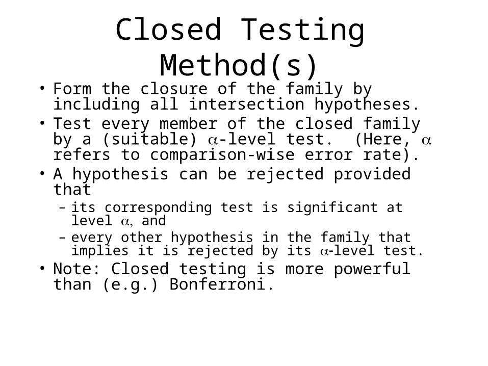
Closed Testing Method(s)• Form the closure of the family by including all

intersection hypotheses.• Test every member of the closed family by a

(suitable) -level test. (Here, refers to comparison-wise error rate).

• A hypothesis can be rejected provided that– its corresponding test is significant at level and – every other hypothesis in the family that implies it

is rejected by its level test.• Note: Closed testing is more powerful than

(e.g.) Bonferroni.

Control of FWE with Closed Tests

Suppose H0j1,..., H0jm all are true (unknown to you which

ones).

You can reject one or more of these only when you reject the intersection H0j1

... H0jm

Thus, P(reject at least one of H0j1,..., H0jm |

H0j1,..., H0jm all are true)

P(reject H0j1... H0jm |

H0j1,..., H0jm all are true) =

Closed Testing – Multiple EndpointsH0: 1=2=3=4 =0

H0: 1=2=3 =0 H0: 1=2=4 =0 H0: 1=3=4 =0 H0: 2=3=4 =0

H0: 1=2 =0 H0: 1=3 =0 H0: 1=4 =0 H0: 2=3 =0 H0: 2=4 =0 H0: 3=4 =0

H0: 1=0p = 0.0121

H0: 2=0p = 0.0142

H0: 3=0p = 0.1986

H0: 4=0p = 0.0191

Where j = mean difference, treatment -control, endpoint j.

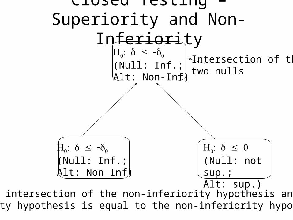
Closed Testing – Superiority and Non-Inferiority

(Null: Inf.;Alt: Non-Inf)

(Null: not sup.;Alt: sup.)

Note: The intersection of the non-inferiority hypothesis and the superiority hypothesis is equal to the non-inferiority hypothesis

(Null: Inf.;Alt: Non-Inf)

Intersection of the two nulls

Why there is no penalty from the closed testing standpoint

• Reject only if

– is rejected, and

– is rejected. (no additional penalty)

• Reject only if

– is rejected, and

– is rejected. (no additional penalty)

So both can be tested at 0.05; sequence is irrelevant.

Why there is no need for multiplicity adjustment: The Partitioning View

• Partitioning principle: – Partition the parameter space into disjoint

subsets of interest– Test each subset using an -level test.– Since the parameter may lie in only one

subset, no multiplicity adjustment is needed.

• Benefits– Can (rarely) be more powerful than closure– Confidence set equivalence (invert the tests)

Partitioning Null Sets

•

•

You may test both without multiplicity adjustment, since only one can be true.

LFC for is ; the LFC for is

Exactly equivalent to closed testing.

Confidence Interval Viewpoint

• Contruct a 1- lower confidence bound on , call it dL.

• If dL > 0, conclude superiority. If dL > conclude non-inferiority.

The testing and interval approaches are essentially equivalent, with possible minor differences where tests and intervals do not coincide (eg, binomial tests).

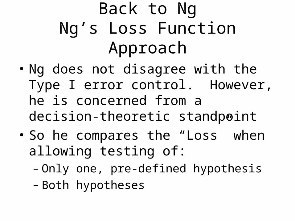
Back to NgNg’s Loss Function Approach

• Ng does not disagree with the Type I error control. However, he is concerned from a decision-theoretic standpoint

• So he compares the “Loss” when allowing testing of: – Only one, pre-defined hypothesis– Both hypotheses

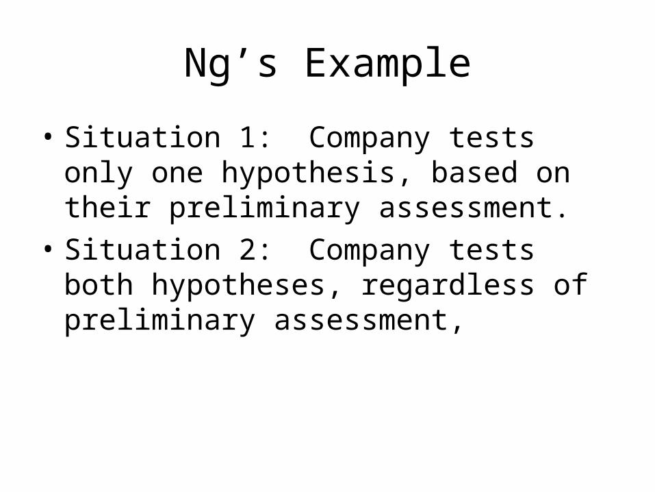
Ng’s Example

• Situation 1: Company tests only one hypothesis, based on their preliminary assessment.

• Situation 2: Company tests both hypotheses, regardless of preliminary assessment,

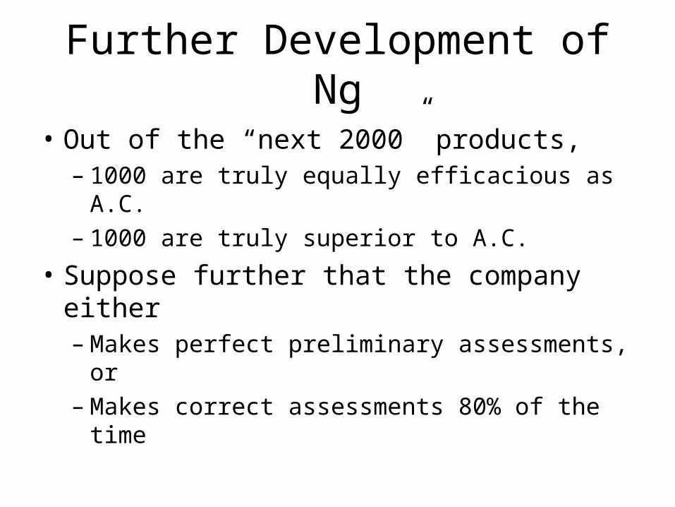
Further Development of Ng

• Out of the “next 2000” products,– 1000 are truly equally efficacious as A.C.– 1000 are truly superior to A.C.

• Suppose further that the company either– Makes perfect preliminary assessments, or– Makes correct assessments 80% of the time

Perfect Classification;One Test Only

Non-Inf. SuperiorityEquivalent 1000 0Superior 0 1000

Type I errors (2.5% level test)Equivalent 0 0Superior 0 0

Type II errors (90% power)Equivalent 100 0Superior 0 100

True State

CompanyTest

True State

True State

80% Correct Classification;One Test Only

Non-Inf. SuperiorityEquivalent 800 200Superior 200 800

Equivalent 0 5Superior 0 0

Equivalent 80 0Superior 0.001 80

True State

Type I errors (2.5% level test)

Type II errors (90% power)

CompanyTest

True State

True State

No Classification;Both Tests Performed

Non.-inf. & SuperiorityEquivalentSuperior

Type I errors (2.5% level test)EquivalentSuperior

Type II errors (90% power)EquivalentSuperior

Test

True State

True State

True State

10001000

25 (superiority claims)0

100 (Fail to claim non-inf)100 (Fail to claim superiority)

Company

Ng’s concern: “Too many” Type I errors.

Westfall’s generalization of Ng

• Three – decision problem:– Superiority– Non-Inferiority– NS (“Inferiority”)

• Usual “Test both” strategy: – Claim Sup if 1.96 < Z

– Claim NonInf if 1.96 –0 < Z < 1.96

– Claim NS if Z < 1.96 –0

Further Development

• Assume 0 = 3.24 (90% power to detect non-inf.).

• True States of Nature– Inferiority: < -3.24– Non-Inf: -3.24 < < 0– Sup: 0 <

Loss Function

0 L12 L13

L21 0 L23

L31 L32 0

Inf (-3.24)

NonInf

(-3.24 < 0)

Sup (0 < )

Nat

ure

Claim

NS NonInf Sup

Prior Distribution –Normal + Equivalence Spike

0

0.2

-10 -5 0 5 10

Westfall’s Extension

• Compare – Ng’s recommendation to “preclassify” drugs

according to Non-Inf or Sup, and– The “test both” recommendation

• Use % increase over minimum loss as a criteria.

• The comparison will depend on prior and loss!

Probability of Selecting “NonInf” Test

0

0.2

0.4

0.6

0.8

1

-6.48 -3.24 0 3.24 6.48

Probit function, anchors are P(NonInf| =0) = ps; P(NonInf| =3.24) = 1-ps.Ng suggests ps=.80.

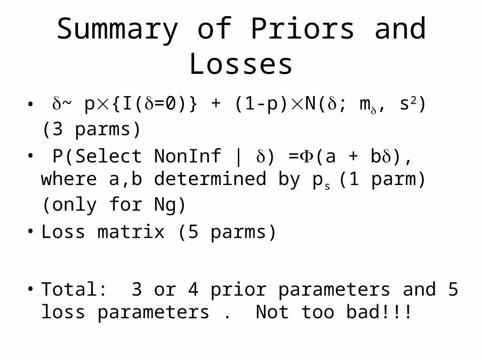
Summary of Priors and Losses

• ~ p{I(=0)} + (1-p)N(; m, s2) (3 parms)

• P(Select NonInf | ) =(a + b), where a,b determined by ps (1 parm) (only for Ng)

• Loss matrix (5 parms)

• Total: 3 or 4 prior parameters and 5 loss parameters . Not too bad!!!

Baseline Model

• ~ (.2){I(=0)} + (.8)N(; 1, 42) • P(Select NonInf | ) =(.84 - .52) (ps=.8)• Loss matrix: (An attempt to quantify “Loss to

patient population”)

0 90 100

1 0 90

20 10 0

Inf (-3.24)

NonInf (-3.24 < 0)

Sup (0 < )

NS/Inf NonInf Sup

Nat

ure

Claim

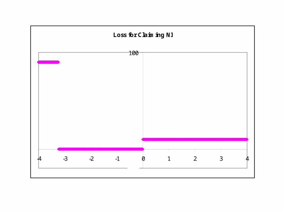
Loss for Claiming NS

-20

100

-4 -3 -2 -1 0 1 2 3 4

Loss for Claiming NI

-20

100

-4 -3 -2 -1 0 1 2 3 4

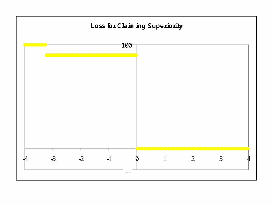
Loss for Claiming Superiority

-20

100

-4 -3 -2 -1 0 1 2 3 4

All Three Loss Functions

-20

100

-4 -2 0 2 4

(ncp)

Lo

ss LNS

LNI

LS

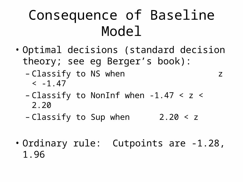
Consequence of Baseline Model

• Optimal decisions (standard decision theory; see eg Berger’s book): – Classify to NS when z < -1.47– Classify to NonInf when -1.47 < z < 2.20– Classify to Sup when 2.20 < z

• Ordinary rule: Cutpoints are -1.28, 1.96

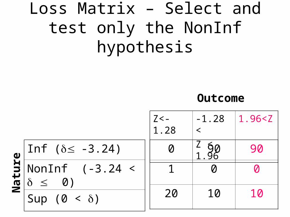
Loss Matrix – Select and test only the NonInf hypothesis

0 90 90

1 0 0

20 10 10

Inf (-3.24)

NonInf (-3.24 < 0)

Sup (0 < )

Z<-1.28 -1.28 <

Z < 1.96

1.96<Z

Nat

ure

Outcome

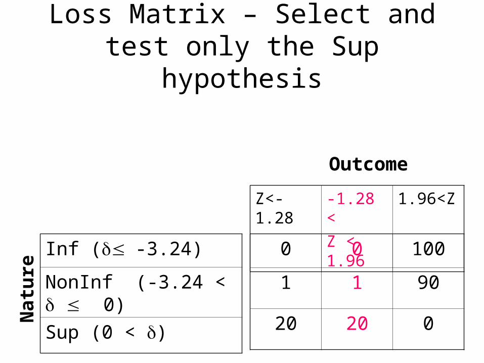
Loss Matrix – Select and test only the Sup hypothesis

0 0 100

1 1 90

20 20 0

Inf (-3.24)

NonInf (-3.24 < 0)

Sup (0 < )

Z<-1.28 -1.28 <

Z < 1.96

1.96<Z

Nat

ure

Outcome

Deviation from Baseline:Effect of p

Loss relative to Optimal

1

1.2

1.4

1.6

1.8

2

0 0.2 0.4 0.6

p=proportion equivalent

Ra

tio Test3

Ng

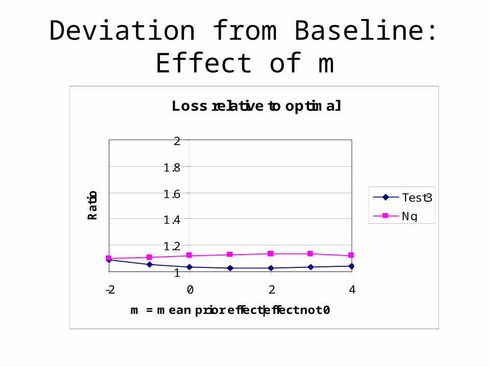
Deviation from Baseline:Effect of m

Loss relative to optimal

1

1.2

1.4

1.6

1.8

2

-2 0 2 4

m = mean prior effect|effect not 0

Rati

o Test3

Ng

Deviation from Baseline:Effect of s

Loss relative to optimal

1

1.2

1.4

1.6

1.8

2

0 2 4 6 8

s = std dev effect size

Ra

tio Test3

Ng

Deviation from Baseline:Effect of Correct Selection, ps

Loss relative to optimal

1

1.2

1.4

1.6

1.8

2

0.5 0.6 0.7 0.8 0.9 1

ps

Rat

io Test3

Ng

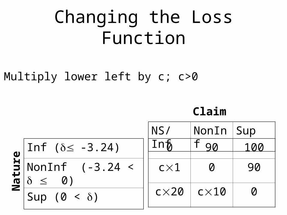
Changing the Loss Function

0 90 100

c1 0 90

c20 c10 0

Inf (-3.24)

NonInf (-3.24 < 0)

Sup (0 < )

NS/Inf NonInf Sup

Nat

ure

Claim

Multiply lower left by c; c>0

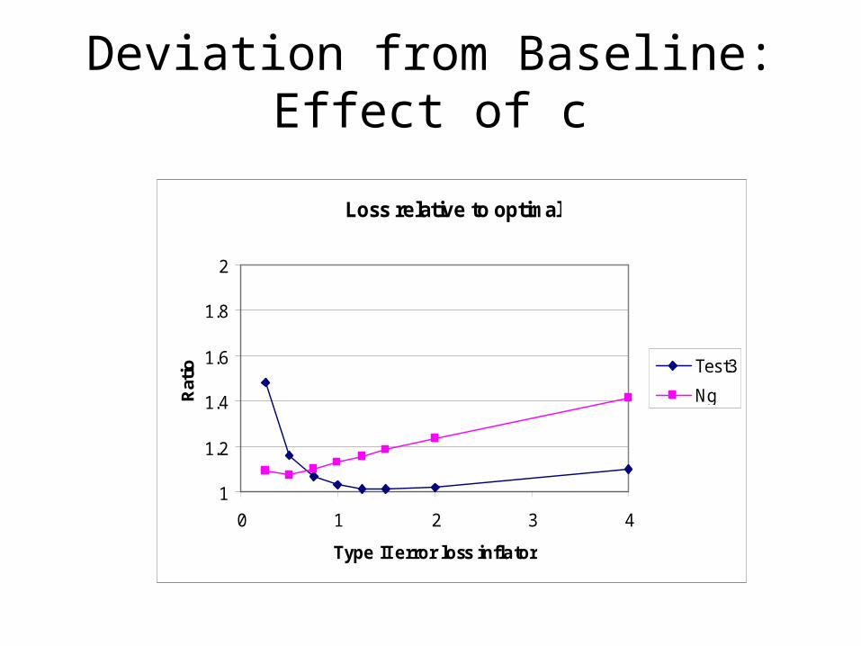
Deviation from Baseline:Effect of c

Loss relative to optimal

1

1.2

1.4

1.6

1.8

2

0 1 2 3 4

Type II error loss inflator

Rat

io Test3

Ng

Conclusions

• The simultaneous testing procedure is generally more efficient (less loss) than Ng’s method, except:– When Type II errors are not costly– When a large % of products are equivalent

• A sidelight: The optimal rule itself is worth considering:– Thresholds for Non-Inf are more liberal, which

allows a more stringent definition of non-inferiority margin