Embed Size (px)
Citation preview
Decision Theory: VE for Decision Networks,
Sequential Decisions, Optimal Policies for Sequential
Decisions Alan Mackworth
UBC CS 322 – Decision Theory 3
April 3, 2013
Textbook §9.2.1, 9.3
Announcements (1) • Assignment 4 was due today. • The list of short questions for the final is online … please
use it! • Please submit suggested review topics on Connect for
review lecture(s). • Previous final has been posted. • Additional review lecture(s) and TA hours will be scheduled
before the final, if needed. • TA hours to continue as scheduled during exam period,
unless as posted otherwise to Connect. • Exercise 12, for single-stage Decision Networks, and
Exercise 13, for multi-stage Decision Networks, have been posted on the home page along with AIspace auxiliary files.

Announcements (2) • Teaching Evaluations are online
– You should have received a message about them – Secure, confidential, mobile access
• Your feedback is important! – Allows us to assess and improve the course material – I use it to assess and improve my teaching methods – The department as a whole uses it to shape the curriculum – Teaching evaluation results are important for instructors
• Appointment, reappointment, tenure, promotion and merit, salary – UBC takes them very seriously (now) – Evaluations close at 11:59PM on April 9, 2013.
• Before exam, but instructors can’t see results until after we submit grades – Please do it!
• Take a few minutes and visit https://eval.olt.ubc.ca/science 3
Lecture Overview
• Recap: Single-Stage Decision Problems – Single-Stage decision networks – Variable elimination (VE) for computing the optimal decision
• Sequential Decision Problems – General decision networks – Policies
• Expected Utility and Optimality of Policies
• Computing the Optimal Policy by Variable Elimination
• Summary & Perspectives
4
Recap: Single vs. Sequential Actions • Single Action (aka One-Off Decisions)
– One or more primitive decisions that can be treated as a single macro decision to be made before acting
• Sequence of Actions (Sequential Decisions) – Repeat:
• observe • act
– Agent has to take actions not knowing what the future brings
5
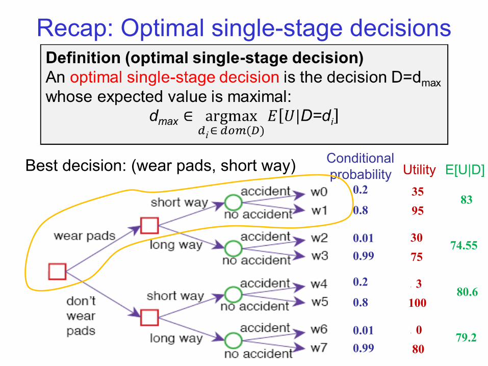
Recap: Optimal single-stage decisions
0.01 0.99
0.2
0.8
0.01 0.99
0.2
0.8
Utility 35 35 95
Conditional probability E[U|D]
83
35 30 75
35 3 100
35 0 80
74.55
80.6
79.2
Best decision: (wear pads, short way)
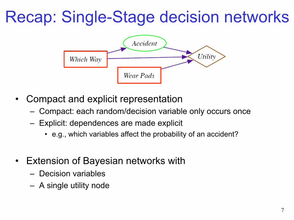
Recap: Single-Stage decision networks
• Compact and explicit representation – Compact: each random/decision variable only occurs once – Explicit: dependences are made explicit
• e.g., which variables affect the probability of an accident?
• Extension of Bayesian networks with – Decision variables – A single utility node
7
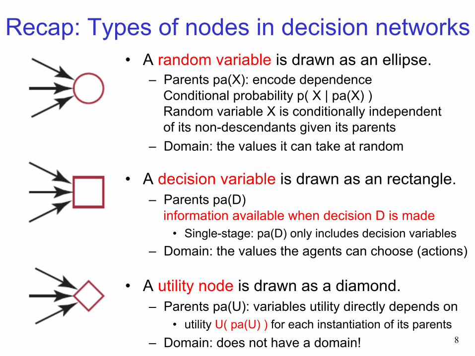
Recap: Types of nodes in decision networks • A random variable is drawn as an ellipse.
– Parents pa(X): encode dependence Conditional probability p( X | pa(X) ) Random variable X is conditionally independent of its non-descendants given its parents
– Domain: the values it can take at random
• A decision variable is drawn as an rectangle. – Parents pa(D)
information available when decision D is made • Single-stage: pa(D) only includes decision variables
– Domain: the values the agents can choose (actions)
• A utility node is drawn as a diamond. – Parents pa(U): variables utility directly depends on
• utility U( pa(U) ) for each instantiation of its parents – Domain: does not have a domain!
8
Lecture Overview
• Recap: Single-Stage Decision Problems – Single-Stage decision networks – Variable elimination (VE) for computing the optimal decision
• Sequential Decision Problems – General decision networks – Policies
• Expected Utility and Optimality of Policies
• Computing the Optimal Policy by Variable Elimination
• Summary & Perspectives
9
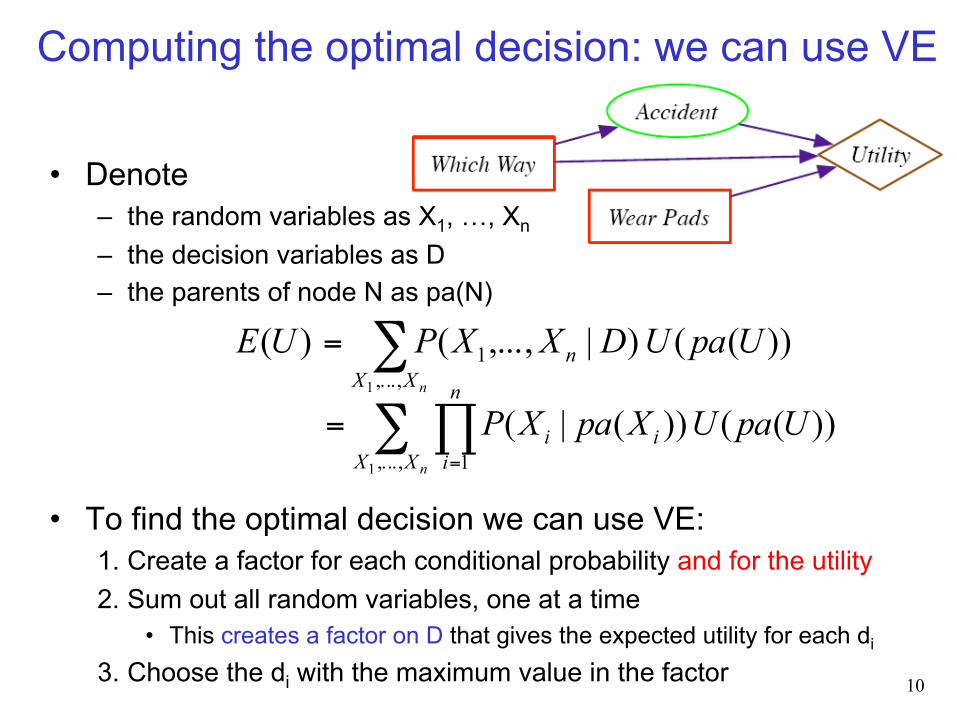
Computing the optimal decision: we can use VE
• Denote – the random variables as X1, …, Xn – the decision variables as D – the parents of node N as pa(N)
• To find the optimal decision we can use VE: 1. Create a factor for each conditional probability and for the utility 2. Sum out all random variables, one at a time
• This creates a factor on D that gives the expected utility for each di
3. Choose the di with the maximum value in the factor
∑=nXX
n UpaUDXXPUE,...,
11
))(()|,...,()(
∑ ∏=
=nXX
n
iii UpaUXpaXP
,..., 11
))(())(|(
10
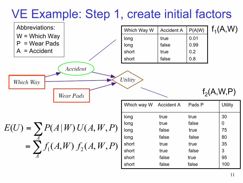
VE Example: Step 1, create initial factors
11
Which way W Accident A Pads P Utility
long true true long true false long false true long false false short true true short true false short false true short false false
30 0 75 80 35 3 95 100
Which Way W Accident A P(A|W) long long short short
true false true false
0.01 0.99 0.2 0.8
f1(A,W)
f2(A,W,P)
∑=A
PWAUWAPUE ),,()|()(
∑=A
PWAfWAf ),,(),( 21
Abbreviations: W = Which Way P = Wear Pads A = Accident
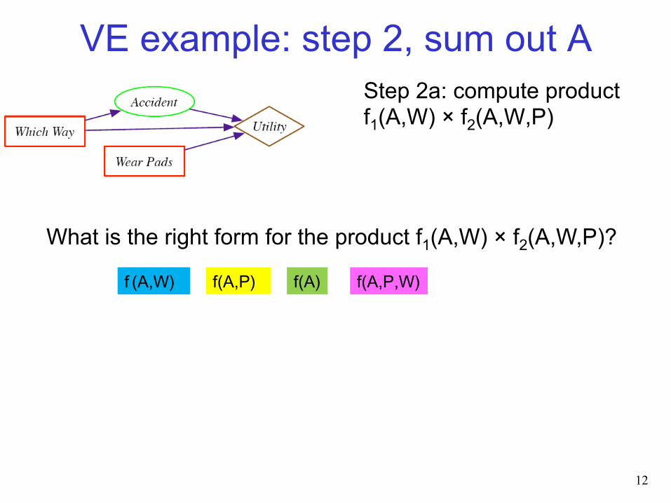
VE example: step 2, sum out A Step 2a: compute product f1(A,W) × f2(A,W,P)
What is the right form for the product f1(A,W) × f2(A,W,P)?
f(A,P) f (A,W) f(A) f(A,P,W)
12
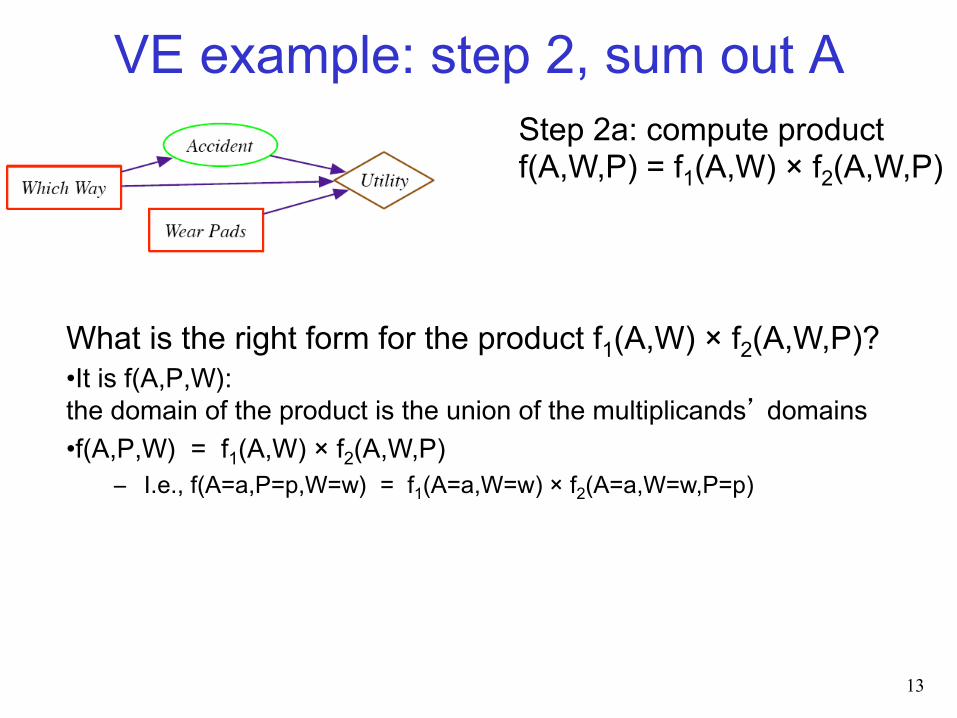
VE example: step 2, sum out A
What is the right form for the product f1(A,W) × f2(A,W,P)? • It is f(A,P,W): the domain of the product is the union of the multiplicands’ domains • f(A,P,W) = f1(A,W) × f2(A,W,P)
– I.e., f(A=a,P=p,W=w) = f1(A=a,W=w) × f2(A=a,W=w,P=p)
13
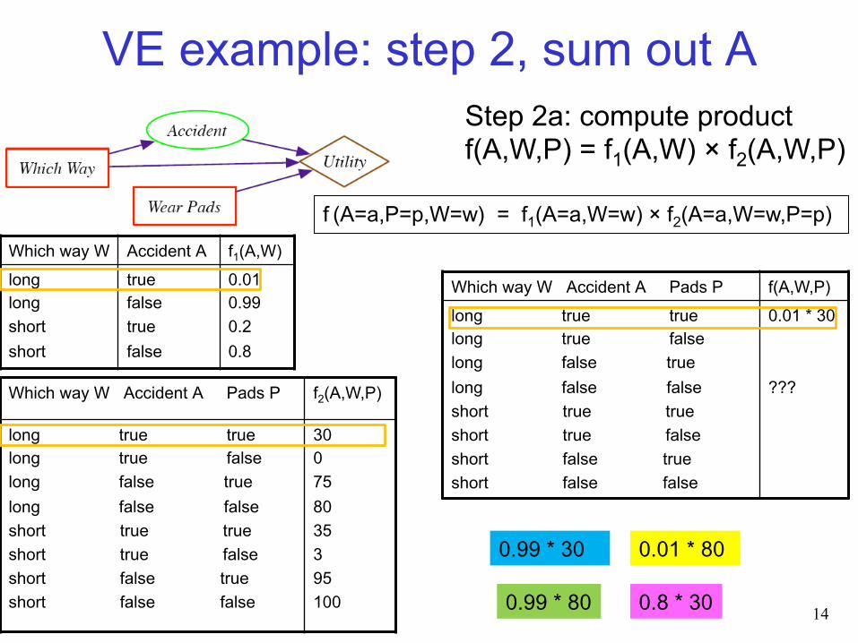
Step 2a: compute product f(A,W,P) = f1(A,W) × f2(A,W,P)
Which way W Accident A Pads P f(A,W,P) long true true long true false long false true long false false short true true short true false short false true short false false
0.01 * 30 ???
VE example: step 2, sum out A
14
Which way W Accident A Pads P f2(A,W,P)
long true true long true false long false true long false false short true true short true false short false true short false false
30 0 75 80 35 3 95 100
Which way W Accident A f1(A,W) long long short short
true false true false
0.01 0.99 0.2 0.8
f (A=a,P=p,W=w) = f1(A=a,W=w) × f2(A=a,W=w,P=p)
0.01 * 80 0.99 * 30
0.99 * 80 0.8 * 30
Step 2a: compute product f(A,W,P) = f1(A,W) × f2(A,W,P)
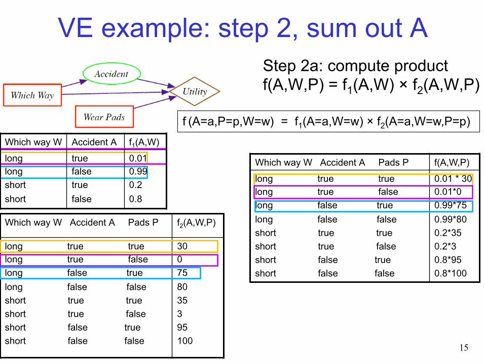
Which way W Accident A Pads P f(A,W,P) long true true long true false long false true long false false short true true short true false short false true short false false
0.01 * 30 0.01*0 0.99*75 0.99*80 0.2*35 0.2*3 0.8*95 0.8*100
VE example: step 2, sum out A Step 2a: compute product f(A,W,P) = f1(A,W) × f2(A,W,P)
15
Which way W Accident A Pads P f2(A,W,P)
long true true long true false long false true long false false short true true short true false short false true short false false
30 0 75 80 35 3 95 100
f (A=a,P=p,W=w) = f1(A=a,W=w) × f2(A=a,W=w,P=p) Which way W Accident A f1(A,W) long long short short
true false true false
0.01 0.99 0.2 0.8
VE example: step 2, sum out A
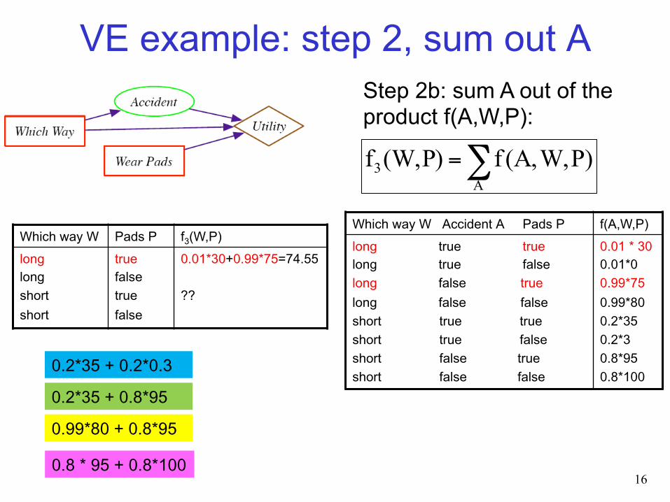
16
Step 2b: sum A out of the product f(A,W,P):
Which way W Pads P f3(W,P) long long short short
true false true false
0.01*30+0.99*75=74.55 ??
∑=A
3 )PW,A,(f P)(W,f
0.99*80 + 0.8*95
0.2*35 + 0.2*0.3
0.2*35 + 0.8*95
0.8 * 95 + 0.8*100
Which way W Accident A Pads P f(A,W,P) long true true long true false long false true long false false short true true short true false short false true short false false
0.01 * 30 0.01*0 0.99*75 0.99*80 0.2*35 0.2*3 0.8*95 0.8*100
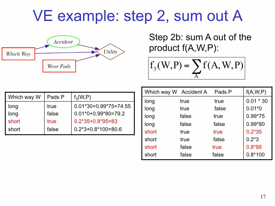
VE example: step 2, sum out A
17
Which way W Pads P f3(W,P) long long short short
true false true false
0.01*30+0.99*75=74.55 0.01*0+0.99*80=79.2 0.2*35+0.8*95=83 0.2*3+0.8*100=80.6
Which way W Accident A Pads P f(A,W,P) long true true long true false long false true long false false short true true short true false short false true short false false
0.01 * 30 0.01*0 0.99*75 0.99*80 0.2*35 0.2*3 0.8*95 0.8*100
Step 2b: sum A out of the product f(A,W,P): ∑=
A3 )PW,A,(f P)(W,f
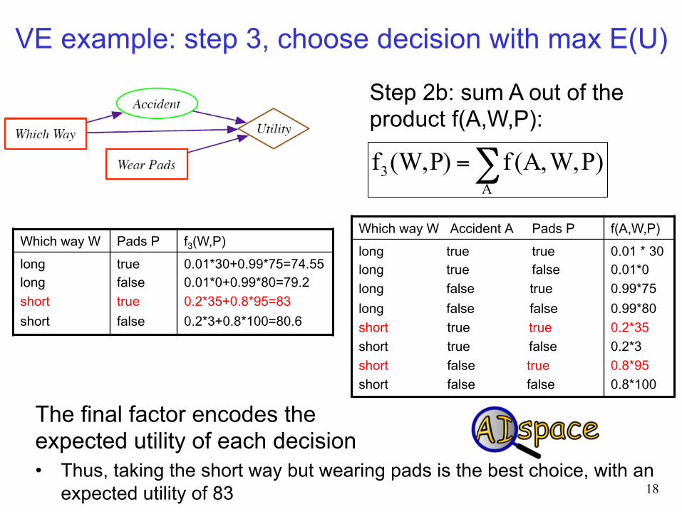
The final factor encodes the expected utility of each decision • Thus, taking the short way but wearing pads is the best choice, with an
expected utility of 83
VE example: step 3, choose decision with max E(U)
18
Which way W Pads P f3(W,P) long long short short
true false true false
0.01*30+0.99*75=74.55 0.01*0+0.99*80=79.2 0.2*35+0.8*95=83 0.2*3+0.8*100=80.6
Which way W Accident A Pads P f(A,W,P) long true true long true false long false true long false false short true true short true false short false true short false false
0.01 * 30 0.01*0 0.99*75 0.99*80 0.2*35 0.2*3 0.8*95 0.8*100
Step 2b: sum A out of the product f(A,W,P): ∑=
A3 )PW,A,(f P)(W,f
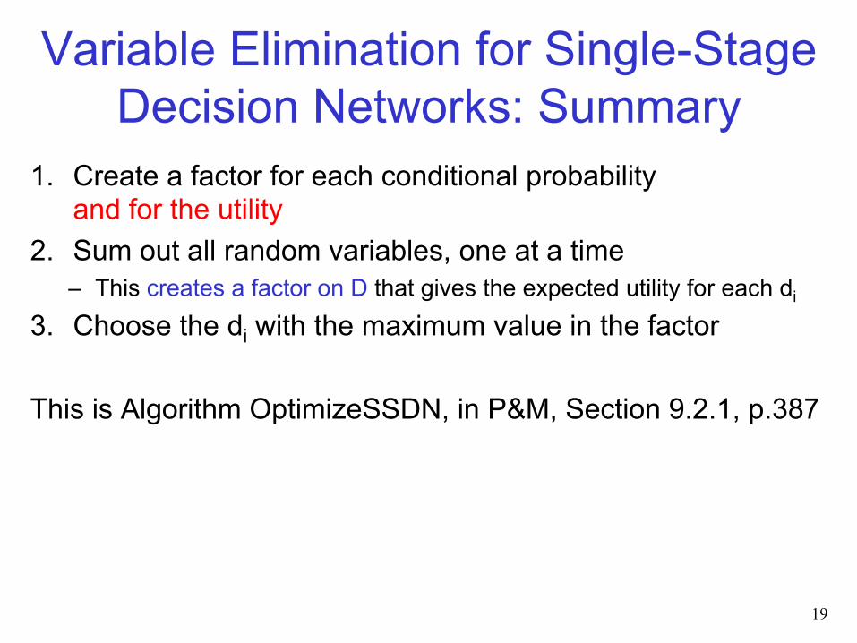
Variable Elimination for Single-Stage
Decision Networks: Summary 1. Create a factor for each conditional probability
and for the utility 2. Sum out all random variables, one at a time
– This creates a factor on D that gives the expected utility for each di 3. Choose the di with the maximum value in the factor
This is Algorithm OptimizeSSDN, in P&M, Section 9.2.1, p.387
19
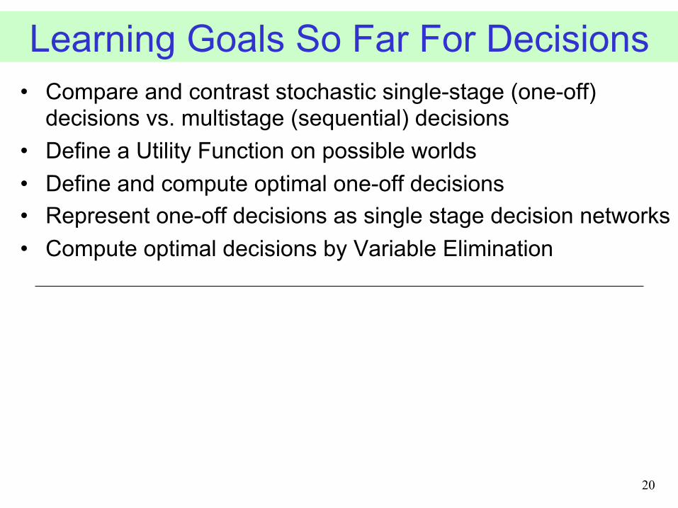
• Compare and contrast stochastic single-stage (one-off) decisions vs. multistage (sequential) decisions
• Define a Utility Function on possible worlds • Define and compute optimal one-off decisions • Represent one-off decisions as single stage decision networks • Compute optimal decisions by Variable Elimination
20
Learning Goals So Far For Decisions
Lecture Overview
• Recap: Single-Stage Decision Problems – Single-Stage decision networks – Variable elimination (VE) for computing the optimal decision
• Sequential Decision Problems – General decision networks – Policies
• Expected Utility and Optimality of Policies
• Computing the Optimal Policy by Variable Elimination
• Summary & Perspectives
21
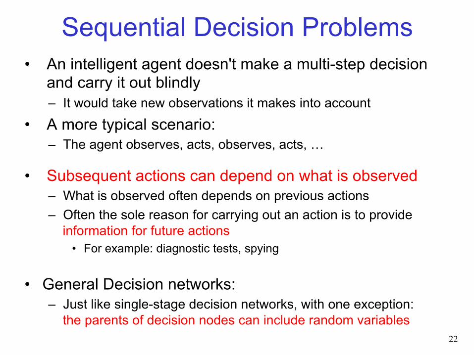
Sequential Decision Problems • An intelligent agent doesn't make a multi-step decision
and carry it out blindly – It would take new observations it makes into account
• A more typical scenario: – The agent observes, acts, observes, acts, …
• Subsequent actions can depend on what is observed – What is observed often depends on previous actions – Often the sole reason for carrying out an action is to provide
information for future actions • For example: diagnostic tests, spying
• General Decision networks: – Just like single-stage decision networks, with one exception:
the parents of decision nodes can include random variables 22
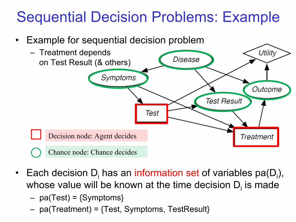
Sequential Decision Problems: Example • Example for sequential decision problem
– Treatment depends on Test Result (& others)
• Each decision Di has an information set of variables pa(Di), whose value will be known at the time decision Di is made – pa(Test) = {Symptoms} – pa(Treatment) = {Test, Symptoms, TestResult}
Decision node: Agent decides
Chance node: Chance decides
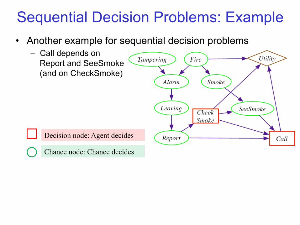
• Another example for sequential decision problems – Call depends on
Report and SeeSmoke (and on CheckSmoke)
Sequential Decision Problems: Example
Decision node: Agent decides
Chance node: Chance decides
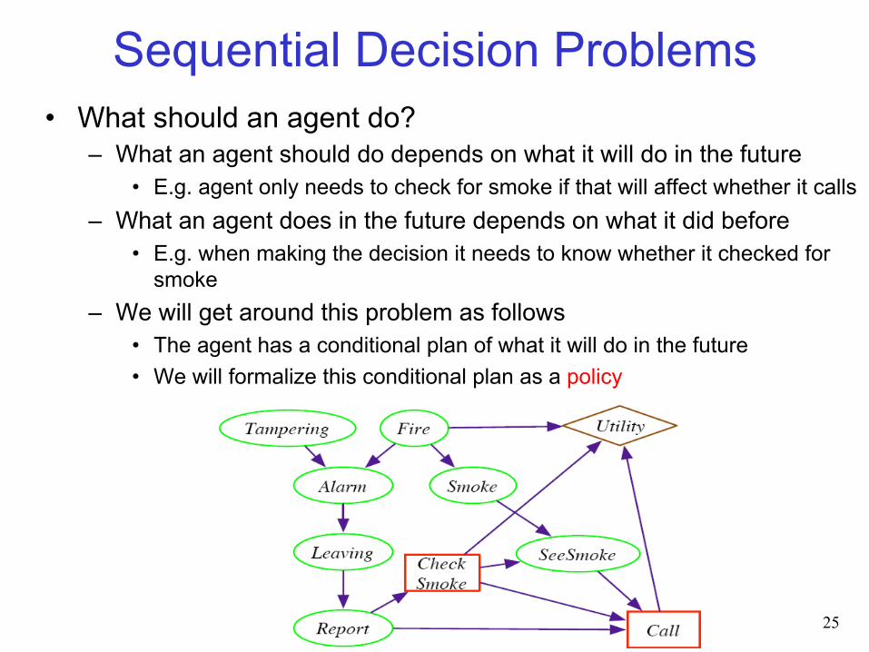
Sequential Decision Problems • What should an agent do?
– What an agent should do depends on what it will do in the future • E.g. agent only needs to check for smoke if that will affect whether it calls
– What an agent does in the future depends on what it did before • E.g. when making the decision it needs to know whether it checked for
smoke – We will get around this problem as follows
• The agent has a conditional plan of what it will do in the future • We will formalize this conditional plan as a policy
25
Policies for Sequential Decision Problems
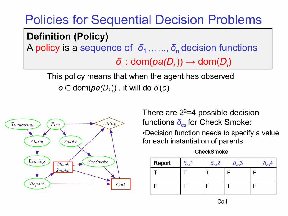
This policy means that when the agent has observed o ∈ dom(pa(Di )) , it will do δi(o)
CheckSmoke
Report δcs1 δcs2 δcs3 δcs4 T T T F F
F T F T F
Call
Definition (Policy) A policy is a sequence of δ1 ,….., δn decision functions
δi : dom(pa(Di )) → dom(Di)
There are 22=4 possible decision functions δcs for Check Smoke: • Decision function needs to specify a value for each instantiation of parents
R=t,CS=t,SS=t"
R=t,CS=t,SS=f"
R=t,CS=f,SS=t"
R=t,CS=f,SS=f"
R=f,CS=t,SS=t"
R=f,CS=t,SS=f"
R=f,CS=f,SS=t"
R=f,CS=f,SS=f"
δcall1(R) T T T T T T T" T"δcall2(R) T T T T T T T" F"δcall3(R) T T T T T T F" T"δcall4(R) T T T T T T F" F"δcall5(R) T T T T T F T" T"… … …" …" …" …" …" …" …"
δcall256(R) F F" F" F" F" F" F" F"
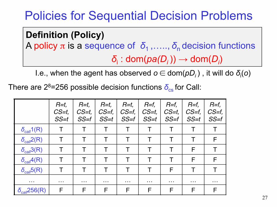
Policies for Sequential Decision Problems Definition (Policy) A policy π is a sequence of δ1 ,….., δn decision functions
δi : dom(pa(Di )) → dom(Di)
There are 28=256 possible decision functions δcs for Call:
I.e., when the agent has observed o ∈ dom(pDi ) , it will do δi(o)
27
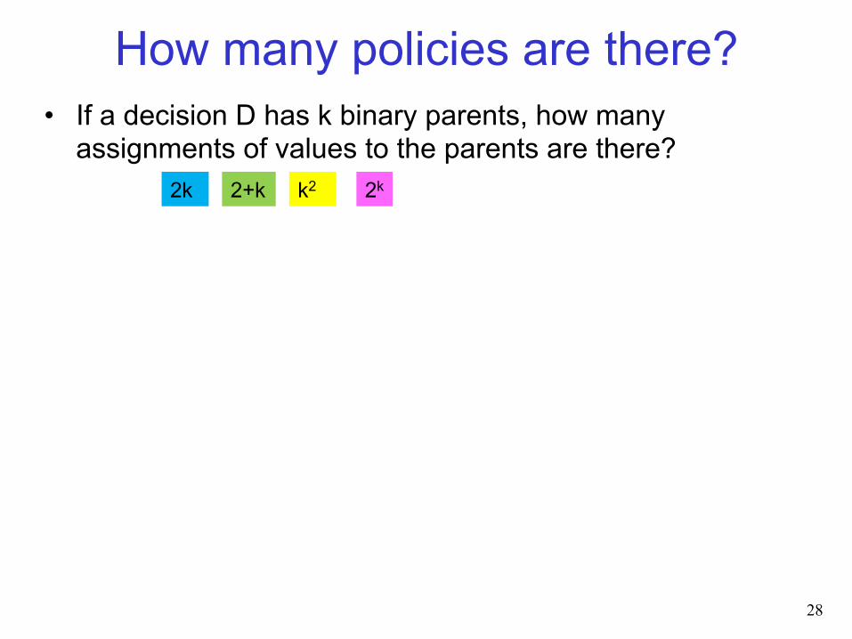
How many policies are there? • If a decision D has k binary parents, how many
assignments of values to the parents are there?
28
k2 2k 2+k 2k
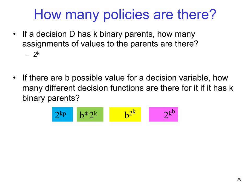
How many policies are there? • If a decision D has k binary parents, how many
assignments of values to the parents are there? – 2k
• If there are b possible value for a decision variable, how many different decision functions are there for it if it has k binary parents?
29
b2k 2kp b*2k 2kb
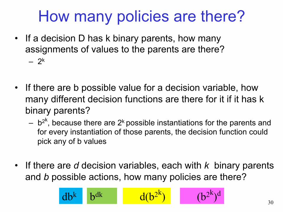
How many policies are there? • If a decision D has k binary parents, how many
assignments of values to the parents are there? – 2k
• If there are b possible value for a decision variable, how many different decision functions are there for it if it has k binary parents? – b2k, because there are 2k possible instantiations for the parents and
for every instantiation of those parents, the decision function could pick any of b values
• If there are d decision variables, each with k binary parents and b possible actions, how many policies are there?
30 d(b2k) dbk bdk (b2k)d
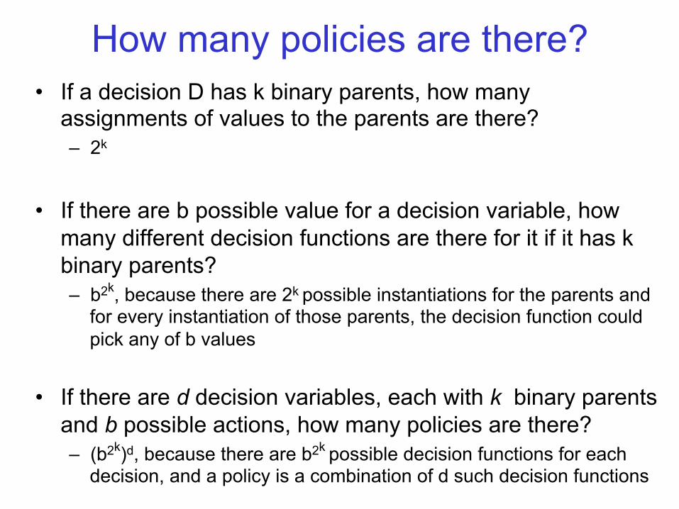
How many policies are there? • If a decision D has k binary parents, how many
assignments of values to the parents are there? – 2k
• If there are b possible value for a decision variable, how many different decision functions are there for it if it has k binary parents? – b2k, because there are 2k possible instantiations for the parents and
for every instantiation of those parents, the decision function could pick any of b values
• If there are d decision variables, each with k binary parents and b possible actions, how many policies are there? – (b2k)d, because there are b2k possible decision functions for each
decision, and a policy is a combination of d such decision functions
Lecture Overview
• Recap: Single-Stage Decision Problems – Single-Stage decision networks – Variable elimination (VE) for computing the optimal decision
• Sequential Decision Problems – General decision networks – Policies
• Expected Utility and Optimality of Policies
• Computing the Optimal Policy by Variable Elimination
• Summary & Perspectives
32
Possible worlds satisfying a policy
33
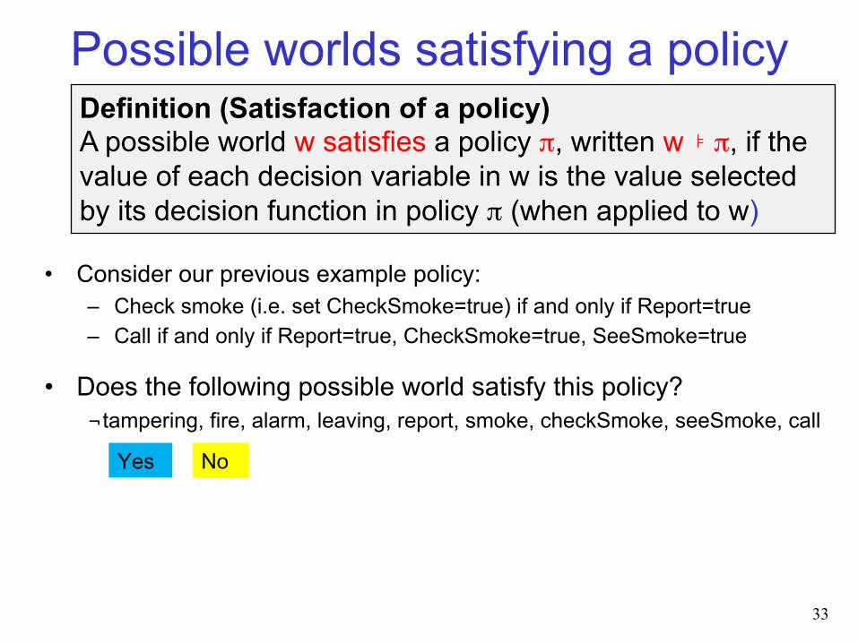
Definition (Satisfaction of a policy) A possible world w satisfies a policy π, written w ⊧ π, if the value of each decision variable in w is the value selected by its decision function in policy π (when applied to w)
• Consider our previous example policy: – Check smoke (i.e. set CheckSmoke=true) if and only if Report=true – Call if and only if Report=true, CheckSmoke=true, SeeSmoke=true
• Does the following possible world satisfy this policy? ¬tampering, fire, alarm, leaving, report, smoke, checkSmoke, seeSmoke, call
No Yes
Possible worlds satisfying a policy
34
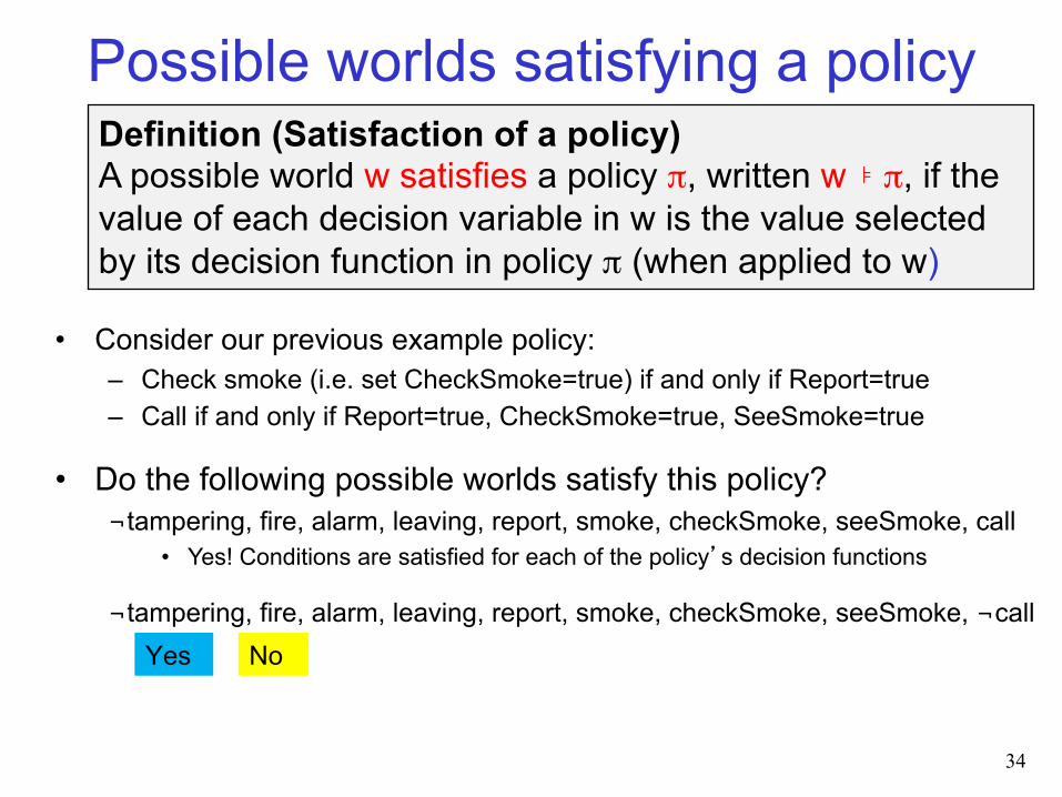
Definition (Satisfaction of a policy) A possible world w satisfies a policy π, written w ⊧ π, if the value of each decision variable in w is the value selected by its decision function in policy π (when applied to w)
• Consider our previous example policy: – Check smoke (i.e. set CheckSmoke=true) if and only if Report=true – Call if and only if Report=true, CheckSmoke=true, SeeSmoke=true
• Do the following possible worlds satisfy this policy? ¬tampering, fire, alarm, leaving, report, smoke, checkSmoke, seeSmoke, call
• Yes! Conditions are satisfied for each of the policy’s decision functions
¬tampering, fire, alarm, leaving, report, smoke, checkSmoke, seeSmoke, ¬call No Yes
Possible worlds satisfying a policy
35
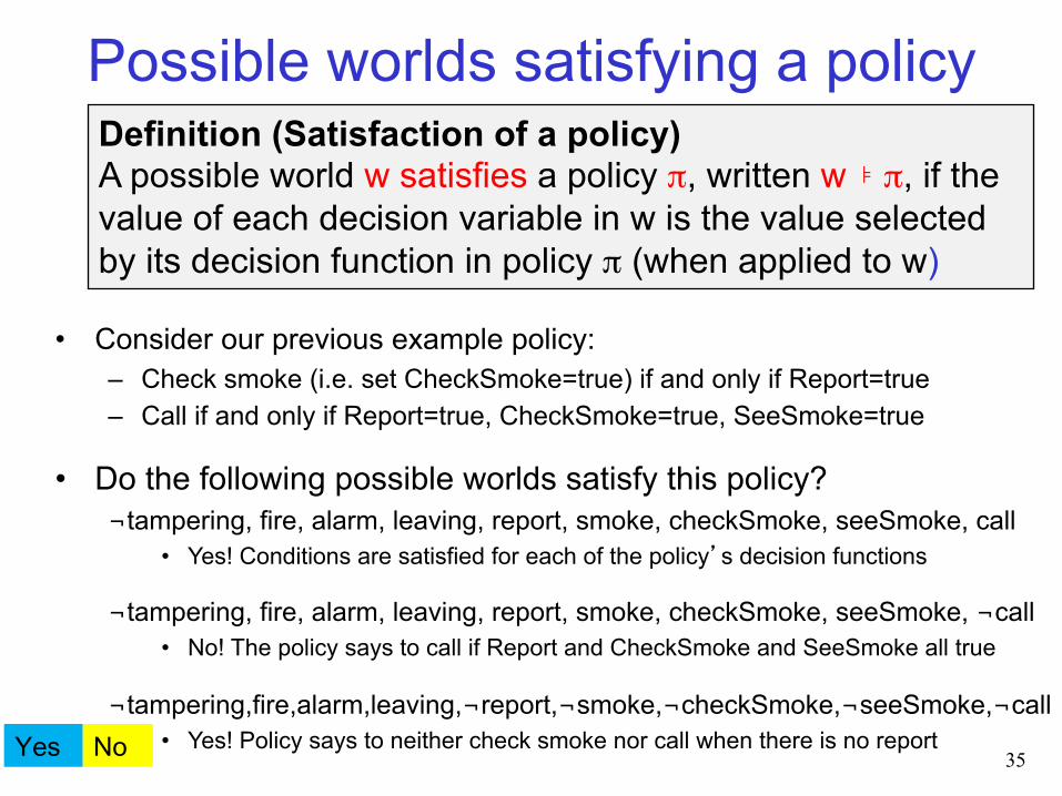
Definition (Satisfaction of a policy) A possible world w satisfies a policy π, written w ⊧ π, if the value of each decision variable in w is the value selected by its decision function in policy π (when applied to w)
• Consider our previous example policy: – Check smoke (i.e. set CheckSmoke=true) if and only if Report=true – Call if and only if Report=true, CheckSmoke=true, SeeSmoke=true
• Do the following possible worlds satisfy this policy? ¬tampering, fire, alarm, leaving, report, smoke, checkSmoke, seeSmoke, call
• Yes! Conditions are satisfied for each of the policy’s decision functions
¬tampering, fire, alarm, leaving, report, smoke, checkSmoke, seeSmoke, ¬call • No! The policy says to call if Report and CheckSmoke and SeeSmoke all true
¬tampering,fire,alarm,leaving,¬report,¬smoke,¬checkSmoke,¬seeSmoke,¬call • Yes! Policy says to neither check smoke nor call when there is no report No Yes
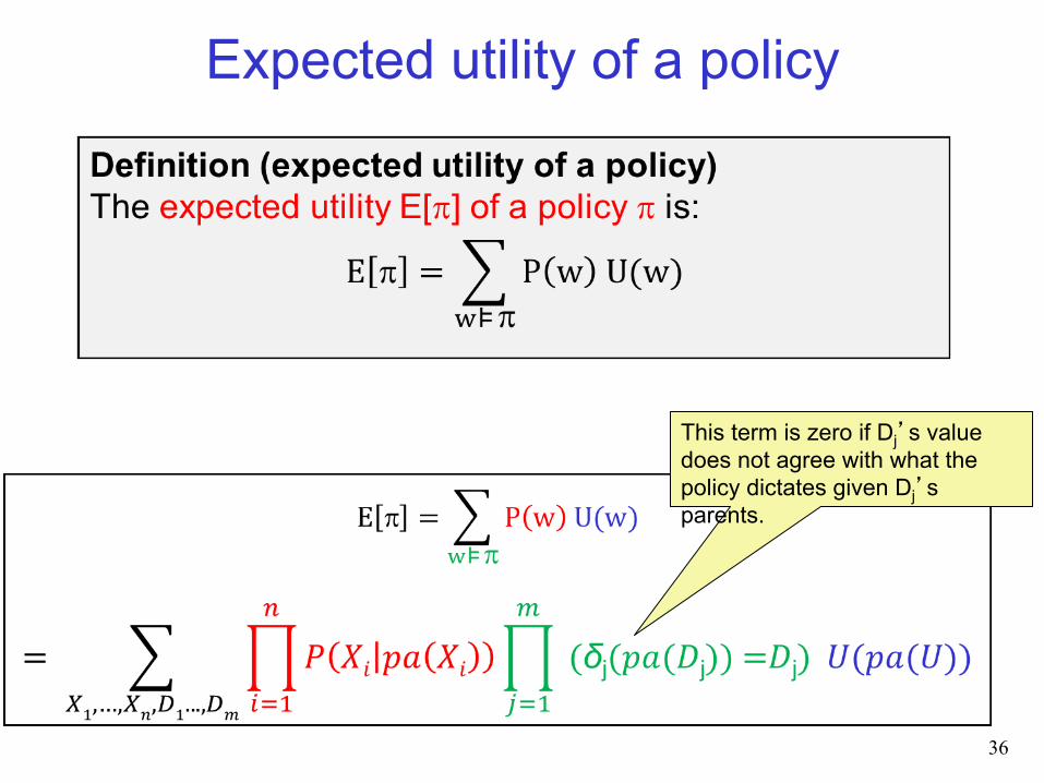
Expected utility of a policy
36
This term is zero if Dj’s value does not agree with what the policy dictates given Dj’s parents.
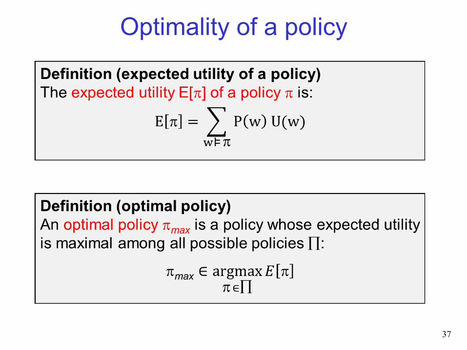
Optimality of a policy
37
Lecture Overview
• Recap: Single-Stage Decision Problems – Single-Stage decision networks – Variable elimination (VE) for computing the optimal decision
• Sequential Decision Problems – General decision networks – Policies
• Expected Utility and Optimality of Policies
• Computing the Optimal Policy by Variable Elimination
• Summary & Perspectives
38
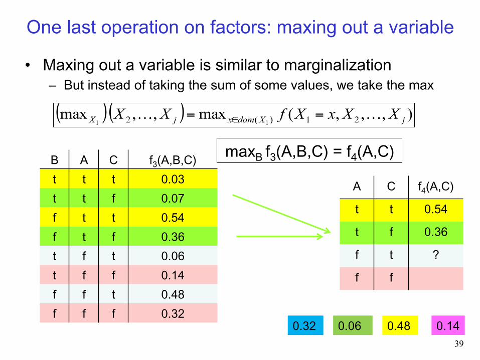
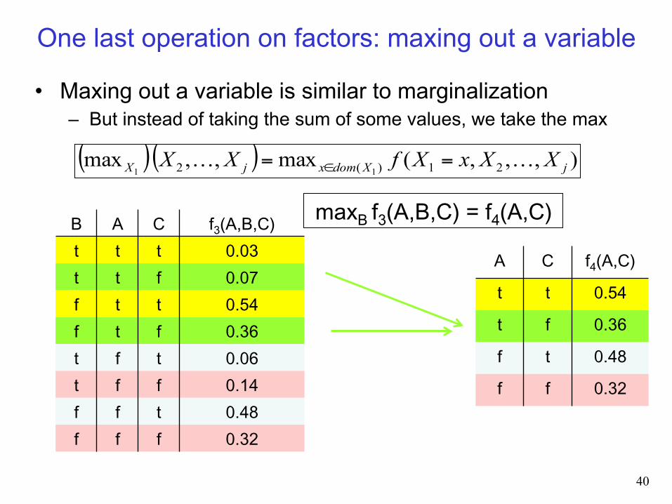
One last operation on factors: maxing out a variable
• Maxing out a variable is similar to marginalization – But instead of taking the sum of some values, we take the max
B A C f3(A,B,C) t t t 0.03 t t f 0.07 f t t 0.54 f t f 0.36 t f t 0.06 t f f 0.14 f f t 0.48 f f f 0.32
A C f4(A,C)
t t 0.54
t f 0.36
f t ?
f f
maxB f3(A,B,C) = f4(A,C)
( )( ) ),,,(max,,max 21)(2 11 jXdomxjX XXxXfXX …… == ∈
0.48 0.32 0.06 0.14
39
One last operation on factors: maxing out a variable
• Maxing out a variable is similar to marginalization – But instead of taking the sum of some values, we take the max
B A C f3(A,B,C) t t t 0.03 t t f 0.07 f t t 0.54 f t f 0.36 t f t 0.06 t f f 0.14 f f t 0.48 f f f 0.32
A C f4(A,C)
t t 0.54
t f 0.36
f t 0.48
f f 0.32
maxB f3(A,B,C) = f4(A,C)
( )( ) ),,,(max,,max 21)(2 11 jXdomxjX XXxXfXX …… == ∈
40
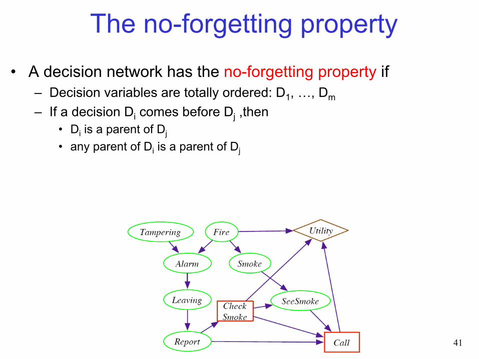
The no-forgetting property
• A decision network has the no-forgetting property if – Decision variables are totally ordered: D1, …, Dm – If a decision Di comes before Dj ,then
• Di is a parent of Dj • any parent of Di is a parent of Dj
41
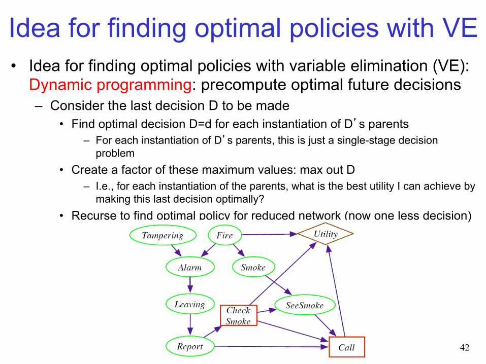
Idea for finding optimal policies with VE • Idea for finding optimal policies with variable elimination (VE):
Dynamic programming: precompute optimal future decisions – Consider the last decision D to be made
• Find optimal decision D=d for each instantiation of D’s parents – For each instantiation of D’s parents, this is just a single-stage decision
problem • Create a factor of these maximum values: max out D
– I.e., for each instantiation of the parents, what is the best utility I can achieve by making this last decision optimally?
• Recurse to find optimal policy for reduced network (now one less decision)
42
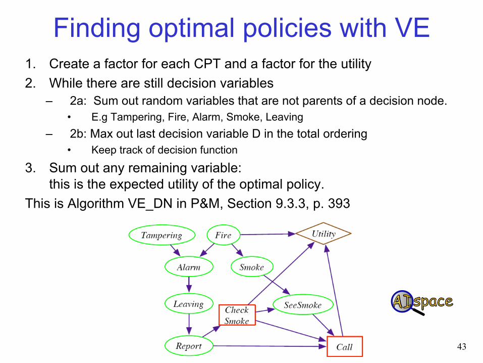
Finding optimal policies with VE 1. Create a factor for each CPT and a factor for the utility 2. While there are still decision variables
– 2a: Sum out random variables that are not parents of a decision node. • E.g Tampering, Fire, Alarm, Smoke, Leaving
– 2b: Max out last decision variable D in the total ordering • Keep track of decision function
3. Sum out any remaining variable: this is the expected utility of the optimal policy.
This is Algorithm VE_DN in P&M, Section 9.3.3, p. 393
43
Computational complexity of VE for
finding optimal policies
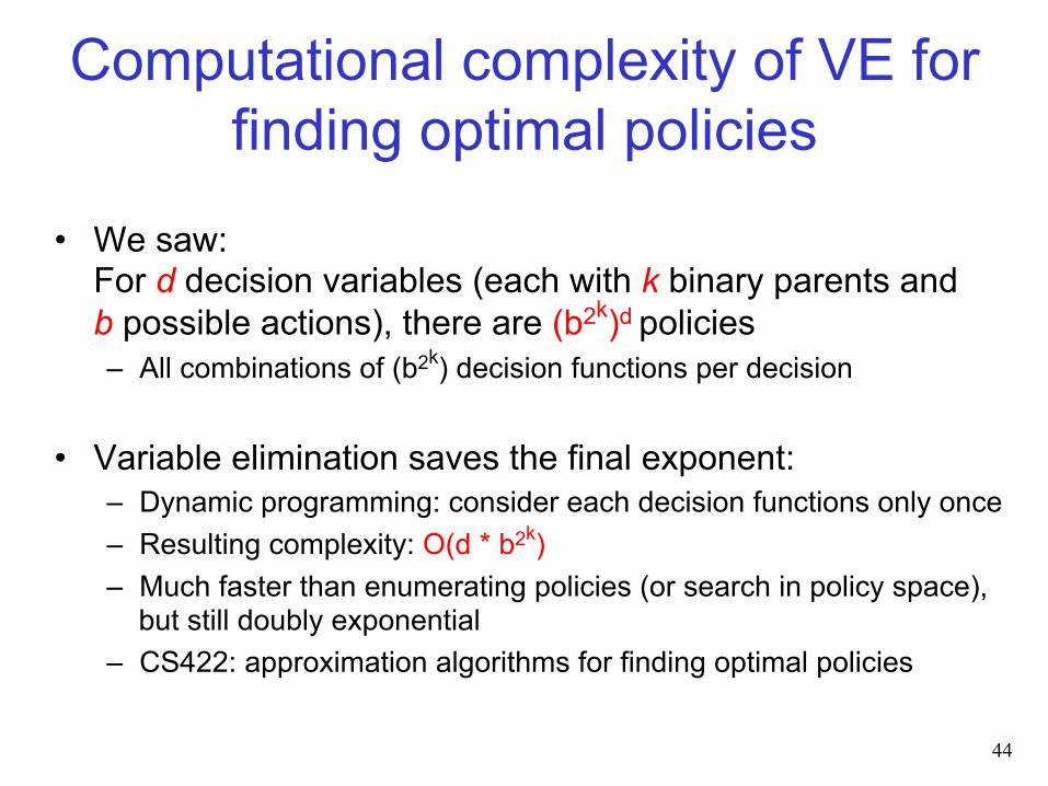
• We saw: For d decision variables (each with k binary parents and b possible actions), there are (b2k)d policies – All combinations of (b2k) decision functions per decision
• Variable elimination saves the final exponent: – Dynamic programming: consider each decision functions only once – Resulting complexity: O(d * b2k)
– Much faster than enumerating policies (or search in policy space), but still doubly exponential
– CS422: approximation algorithms for finding optimal policies
44
Lecture Overview
• Recap: Single-Stage Decision Problems – Single-Stage decision networks – Variable elimination (VE) for computing the optimal decision
• Sequential Decision Problems – General decision networks – Policies
• Expected Utility and Optimality of Policies
• Computing the Optimal Policy by Variable Elimination
• Summary & Perspectives
45
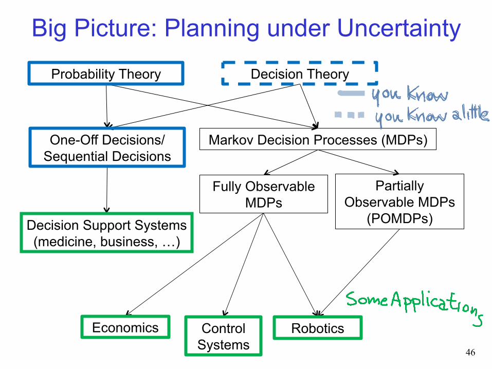
Markov Decision Processes (MDPs)
Big Picture: Planning under Uncertainty
Fully Observable MDPs
Partially Observable MDPs
(POMDPs)
One-Off Decisions/ Sequential Decisions
Probability Theory Decision Theory
Decision Support Systems (medicine, business, …)
Economics Control Systems
Robotics 46
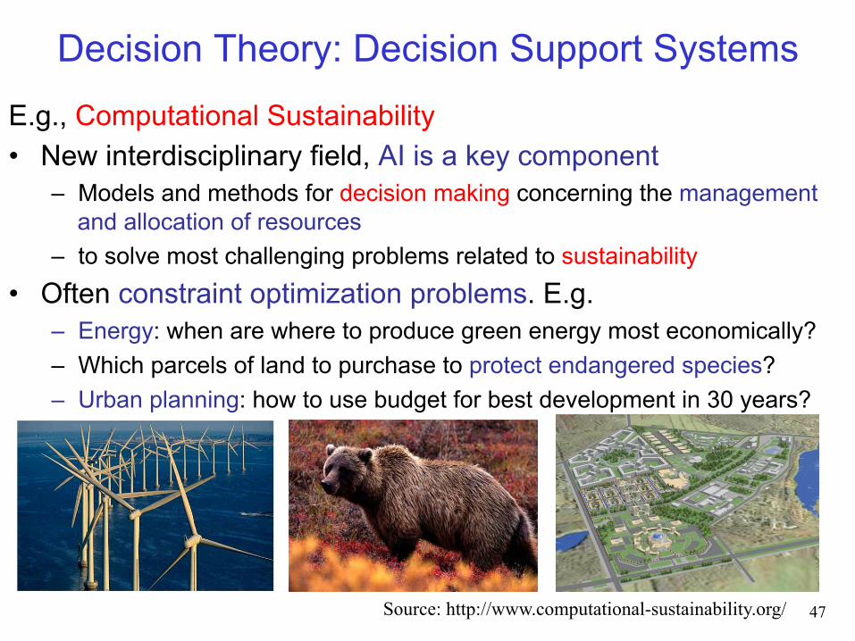
Decision Theory: Decision Support Systems
E.g., Computational Sustainability • New interdisciplinary field, AI is a key component
– Models and methods for decision making concerning the management and allocation of resources
– to solve most challenging problems related to sustainability • Often constraint optimization problems. E.g.
– Energy: when are where to produce green energy most economically? – Which parcels of land to purchase to protect endangered species? – Urban planning: how to use budget for best development in 30 years?
47 Source: http://www.computational-sustainability.org/

Planning Under Uncertainty • Learning and Using
POMDP models of Patient-Caregiver Interactions During Activities of Daily Living
• Goal: Help older adults living with cognitive disabilities (such as Alzheimer's) when they: – forget the proper sequence of
tasks that need to be completed – lose track of the steps that they
have already completed
48
Source: Jesse Hoey UofT 2007
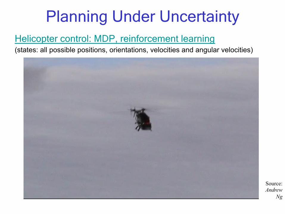
Planning Under Uncertainty
Source: Andrew
Ng
Helicopter control: MDP, reinforcement learning (states: all possible positions, orientations, velocities and angular velocities)
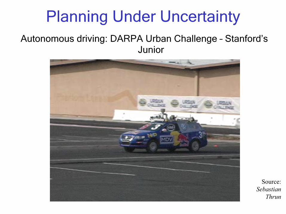
Planning Under Uncertainty Autonomous driving: DARPA Urban Challenge – Stanford’s
Junior
Source: Sebastian
Thrun
• Sequential decision networks – Represent sequential decision problems as decision networks – Explain the non forgetting property
• Policies – Verify whether a possible world satisfies a policy – Define the expected utility of a policy – Compute the number of policies for a decision problem – Compute the optimal policy by Variable Elimination
51
Learning Goals For Today’s Class