Embed Size (px)
Citation preview
POLYTECHNIC UNIVERSITYDepartment of Computer Science / Finance and Risk
Engineering
Decision Trees and Decision Rules
K. Ming Leung
Abstract: The logic-based decision trees and decisionrules methodology performs well across a wide range ofdata mining problems. It also has the advantage thatthe results can be expressed in terms that the end-usercan easily understand.
Directory• Table of Contents• Begin Article
Copyright c© 2007 [email protected] Revision Date: December 6, 2007
Table of Contents
1. Introduction1.1. Motivation and Background
2. C4.5 Algorithm: Generating a Decision Tree2.1. Choice of Test at a Node2.2. Dealing with Features with Numeric Values2.3. An Example: Generating a Decision Tree2.4. The Split-Information parameter2.5. Handling Unknown Attribute Values2.6. Pruning Decision Trees2.7. Advantages and disadvantages
Section 1: Introduction 3
1. Introduction
1.1. Motivation and Background
The logic-based decision trees and decision rules methodology is themost powerful type of off-the-shelf classifiers that performs well acrossa wide range of data mining problems. These classifiers adopt a top-down approach and use supervised learning to construct decision treesfrom a set of given training data set. A decision tree consists ofnodes where attributes are tested. The outgoing branches of the nodecorrespond to all the possible outcomes of the test at the node.
For example, consider samples having two features, X and Y ,where X has continuous real values and Y is a categorical variablehaving three possible values, A, B, and C. The figure shows an ex-ample of a simple decision tree for classifying these samples. Nodesare denoted by circles, and the decision tree (actually an inverted tree)ends at one of the leaves, denoted by rectangles. Each leaf identifiesa particular class. In this example, all samples with features valuesX > 1 and Y = A belong to Class 1. Samples with X > 1 andY = B or C belong to Class 2. Samples with X ≤ 1 belong to Class
Toc JJ II J I Back J Doc Doc I
Section 2: C4.5 Algorithm: Generating a Decision Tree 4
1, regardless of their value for Y .Notice that in this example, at each node a test is performed based
on the value of a single attribute. Decision trees that use univariatesplits have a simple representational form, making it easy for the end-user to understand the inferred model. However at the same time,they represent a restriction on the expressiveness of the model andthus the approximation power of the model.
2. C4.5 Algorithm: Generating a Decision Tree
We will consider the C4.5 algorithm for determining the best decisiontree based on univariate splits. It works with both categorical andnumeric feature values. The algorithm was developed by Ross Quin-lan. It is an extension of his earlier ID3 algorithm. He went on tocreate C5.0 and See5 (C5.0 for Unix/Linux, See5 for Windows) whichhe markets commercially.
There are two stages of the C4.5 algorithm. The first part, which isdiscussed in this section, deals with generating the decision tree basedon the training data set. The second part has to do with pruning the
Toc JJ II J I Back J Doc Doc I
Section 2: C4.5 Algorithm: Generating a Decision Tree 5
decision tree based on the validating samples.We assume that we have a set T of training samples. Let the
possible classes be denoted as {C1, C2, . . . , Ck}. There are three pos-sibilities depending on the content of the set T .
1. T contains one or more samples, all belonging to a single classCj . The decision tree for T is a leaf identifying class Cj .
2. T contains no samples. The decision tree is again a leaf but theclass to be associated with the leaf must be determined frominformation other than T , such as the overall majority class inT . The C4.5 algorithm uses as a criterion the most frequentclass as the parent of the given node.
3. T contains samples that belong to a mixture od classes. It mustbe refined into subsets of samples that are closer to being asingle-class collection of samples. Based on the value of a sin-gle attribute, an appropriate test that has a certain number ofmutually exclusive outcomes {O1, O2, . . . , On} is chosen. T ispartitioned into subsets T1, T2, . . . , Tn, where Ti contains all thesamples in T that have outcome Oi of the chosen test. The de-
Toc JJ II J I Back J Doc Doc I
Section 2: C4.5 Algorithm: Generating a Decision Tree 6
cision tree for T consists of a decision node identifying the testand one branch for each possible outcome.
The same tree-building procedure is applied recursively to eachsubset of training samples, so that the i-th branch leads to the de-cision tree constructed from the subset Ti of training samples. Thesuccessive division of the set of training samples proceeds until all thesubsets consist of sample belonging to a single class.
2.1. Choice of Test at a Node
The decision tree structure is determined by the tests that we chooseto perform at each of the nodes. Different tests, or different orderof their application, will yield different trees. The choice of test at agiven node is based on information theory to minimize the number oftest that will allow a sample to be classified. In other words, we arelooking for a compact decision tree that is consistent with the trainingset.
Exploring all possible trees and selecting the simplest one is in-feasible since the problem is NP-complete. Therefore most decision
Toc JJ II J I Back J Doc Doc I
Section 2: C4.5 Algorithm: Generating a Decision Tree 7
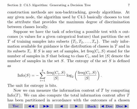
construction methods are non-backtracking, greedy algorithms. Atany given node, the algorithm used by C4.5 basically chooses to testthe attribute that provides the maximum degree of discriminationbetween classes locally.
Suppose we have the task of selecting a possible test with n out-comes (n values for a given categorical feature) that partition the setT of training samples into subsets {T1, T2, . . . , Tn}. The only infor-mation available for guidance is the distribution of classes in T and inits subsets Ti. If S is any set of samples, let freq(Ci, S) stand for thenumber of samples in S that belong to class Ci, and let |S| denote thenumber of samples in the set S. The entropy of the set S is definedas
Info(S) = −k∑
i=1
freq(Ci, S)|S|
log2
(freq(Ci, S)
|S|
).
The unit for entropy is bits.Now we can measure the information content of T by computing
Info(T ). We can also compute the total information content after Thas been partitioned in accordance with the outcomes of a chosen
Toc JJ II J I Back J Doc Doc I
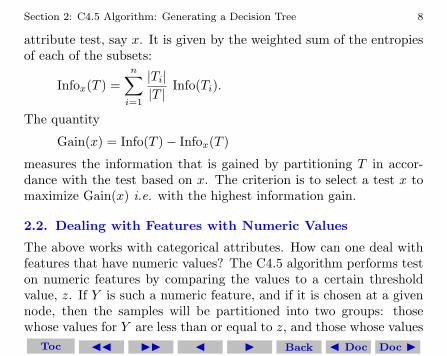
Section 2: C4.5 Algorithm: Generating a Decision Tree 8
attribute test, say x. It is given by the weighted sum of the entropiesof each of the subsets:
Infox(T ) =n∑
i=1
|Ti||T |
Info(Ti).
The quantity
Gain(x) = Info(T )− Infox(T )
measures the information that is gained by partitioning T in accor-dance with the test based on x. The criterion is to select a test x tomaximize Gain(x) i.e. with the highest information gain.
2.2. Dealing with Features with Numeric Values
The above works with categorical attributes. How can one deal withfeatures that have numeric values? The C4.5 algorithm performs teston numeric features by comparing the values to a certain thresholdvalue, z. If Y is such a numeric feature, and if it is chosen at a givennode, then the samples will be partitioned into two groups: thosewhose values for Y are less than or equal to z, and those whose values
Toc JJ II J I Back J Doc Doc I
Section 2: C4.5 Algorithm: Generating a Decision Tree 9
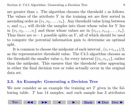
are greater than z. The algorithm chooses the threshold z as follows.The values of the attribute Y in the training set are first sorted inascending order as {v1, v2, . . . , vn}. Any threshold value lying betweenvi and vi+1 will divide the samples into those whose value for Y liesin {v1, v2, . . . , vi} and those whose values are in {vi+1, vi+2, . . . , vn}.Thus there are m−1 possible splits on Y , all of which should be usedto compute the potential information gain to determine an optimalsplit.
It is common to choose the midpoint of each interval , (vi+vi+1)/2,as the representative threshold value. The C4.5 algorithm chooses asthe threshold the smaller value vi for every interval {(vi, vi+1}, ratherthan the midpoint. This ensures that the threshold value appearingin either the final decision tree or rules actually occur in the originaldata set.
2.3. An Example: Generating a Decision Tree
We now consider as an example the training set T given in the fol-lowing table. T has 14 samples, and each sample has 3 attributes
Toc JJ II J I Back J Doc Doc I
Section 2: C4.5 Algorithm: Generating a Decision Tree 10
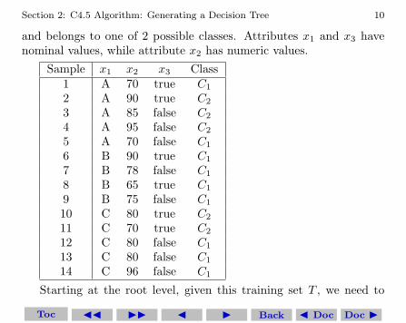
and belongs to one of 2 possible classes. Attributes x1 and x3 havenominal values, while attribute x2 has numeric values.
Sample x1 x2 x3 Class1 A 70 true C1
2 A 90 true C2
3 A 85 false C2
4 A 95 false C2
5 A 70 false C1
6 B 90 true C1
7 B 78 false C1
8 B 65 true C1
9 B 75 false C1
10 C 80 true C2
11 C 70 true C2
12 C 80 false C1
13 C 80 false C1
14 C 96 false C1
Starting at the root level, given this training set T , we need to
Toc JJ II J I Back J Doc Doc I
Section 2: C4.5 Algorithm: Generating a Decision Tree 11
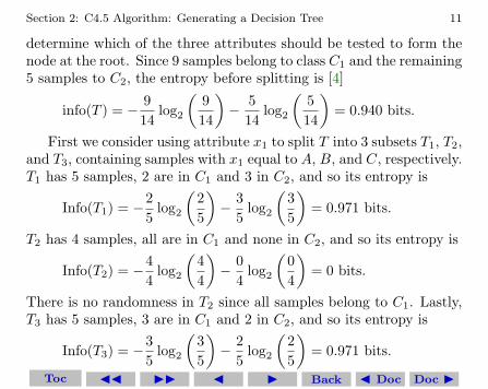
determine which of the three attributes should be tested to form thenode at the root. Since 9 samples belong to class C1 and the remaining5 samples to C2, the entropy before splitting is [4]
info(T ) = − 914
log2
(914
)− 5
14log2
(514
)= 0.940 bits.
First we consider using attribute x1 to split T into 3 subsets T1, T2,and T3, containing samples with x1 equal to A, B, and C, respectively.T1 has 5 samples, 2 are in C1 and 3 in C2, and so its entropy is
Info(T1) = −25
log2
(25
)− 3
5log2
(35
)= 0.971 bits.
T2 has 4 samples, all are in C1 and none in C2, and so its entropy is
Info(T2) = −44
log2
(44
)− 0
4log2
(04
)= 0 bits.
There is no randomness in T2 since all samples belong to C1. Lastly,T3 has 5 samples, 3 are in C1 and 2 in C2, and so its entropy is
Info(T3) = −35
log2
(35
)− 2
5log2
(25
)= 0.971 bits.
Toc JJ II J I Back J Doc Doc I
Section 2: C4.5 Algorithm: Generating a Decision Tree 12
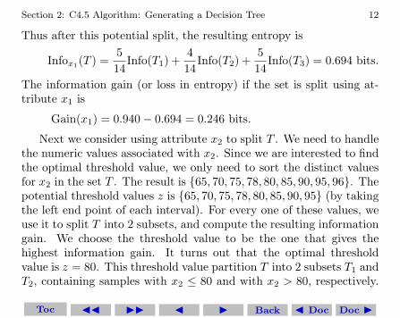
Thus after this potential split, the resulting entropy is
Infox1(T ) =514
Info(T1) +414
Info(T2) +514
Info(T3) = 0.694 bits.
The information gain (or loss in entropy) if the set is split using at-tribute x1 is
Gain(x1) = 0.940− 0.694 = 0.246 bits.
Next we consider using attribute x2 to split T . We need to handlethe numeric values associated with x2. Since we are interested to findthe optimal threshold value, we only need to sort the distinct valuesfor x2 in the set T . The result is {65, 70, 75, 78, 80, 85, 90, 95, 96}. Thepotential threshold values z is {65, 70, 75, 78, 80, 85, 90, 95} (by takingthe left end point of each interval). For every one of these values, weuse it to split T into 2 subsets, and compute the resulting informationgain. We choose the threshold value to be the one that gives thehighest information gain. It turns out that the optimal thresholdvalue is z = 80. This threshold value partition T into 2 subsets T1 andT2, containing samples with x2 ≤ 80 and with x2 > 80, respectively.
Toc JJ II J I Back J Doc Doc I
Section 2: C4.5 Algorithm: Generating a Decision Tree 13
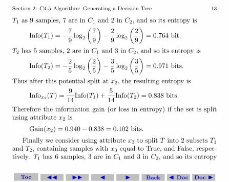
T1 as 9 samples, 7 are in C1 and 2 in C2, and so its entropy is
Info(T1) = −79
log2
(79
)− 2
9log2
(29
)= 0.764 bit.
T2 has 5 samples, 2 are in C1 and 3 in C2, and so its entropy is
Info(T2) = −25
log2
(25
)− 3
5log2
(35
)= 0.971 bits.
Thus after this potential split at x2, the resulting entropy is
Infox2(T ) =914
Info(T1) +514
Info(T2) = 0.838 bits.
Therefore the information gain (or loss in entropy) if the set is splitusing attribute x2 is
Gain(x2) = 0.940− 0.838 = 0.102 bits.
Finally we consider using attribute x3 to split T into 2 subsets T1
and T2, containing samples with x3 equal to True, and False, respec-tively. T1 has 6 samples, 3 are in C1 and 3 in C2, and so its entropy
Toc JJ II J I Back J Doc Doc I
Section 2: C4.5 Algorithm: Generating a Decision Tree 14
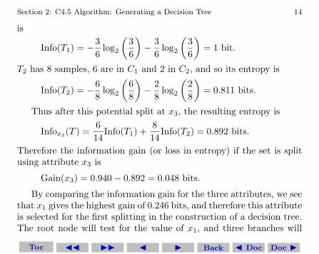
is
Info(T1) = −36
log2
(36
)− 3
6log2
(36
)= 1 bit.
T2 has 8 samples, 6 are in C1 and 2 in C2, and so its entropy is
Info(T2) = −68
log2
(68
)− 2
8log2
(28
)= 0.811 bits.
Thus after this potential split at x3, the resulting entropy is
Infox3(T ) =614
Info(T1) +814
Info(T2) = 0.892 bits.
Therefore the information gain (or loss in entropy) if the set is splitusing attribute x3 is
Gain(x3) = 0.940− 0.892 = 0.048 bits.
By comparing the information gain for the three attributes, we seethat x1 gives the highest gain of 0.246 bits, and therefore this attributeis selected for the first splitting in the construction of a decision tree.The root node will test for the value of x1, and three branches will
Toc JJ II J I Back J Doc Doc I
Section 2: C4.5 Algorithm: Generating a Decision Tree 15
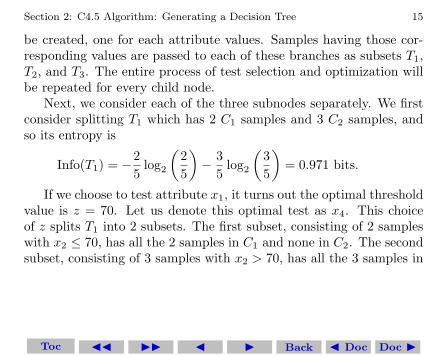
be created, one for each attribute values. Samples having those cor-responding values are passed to each of these branches as subsets T1,T2, and T3. The entire process of test selection and optimization willbe repeated for every child node.
Next, we consider each of the three subnodes separately. We firstconsider splitting T1 which has 2 C1 samples and 3 C2 samples, andso its entropy is
Info(T1) = −25
log2
(25
)− 3
5log2
(35
)= 0.971 bits.
If we choose to test attribute x1, it turns out the optimal thresholdvalue is z = 70. Let us denote this optimal test as x4. This choiceof z splits T1 into 2 subsets. The first subset, consisting of 2 sampleswith x2 ≤ 70, has all the 2 samples in C1 and none in C2. The secondsubset, consisting of 3 samples with x2 > 70, has all the 3 samples in
Toc JJ II J I Back J Doc Doc I
Section 2: C4.5 Algorithm: Generating a Decision Tree 16
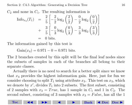
C2 and none in C1. The resulting information is
Infox4(T1) =25
[−2
2log2
(22
)− 0
2log2
(02
)]+
35
[−0
3log2
(03
)− 3
3log2
(33
)]= 0 bits.
The information gained by this test is
Gain(x4) = 0.971− 0 = 0.971 bits.
The 2 branches created by this split will be the final leaf nodes sincethe subsets of samples in each of the branches all belong to theirseparate classes.
Actually there is no need to search for a better split since we knowthat x4 provides the highest information gain. Here, just for fun weconsider choosing to split T1 using attribute x3. This test on x3, whichwe denote by x′, divides T1 into 2 subsets. The first subset, consistingof 2 samples with x3 = True, has 1 sample in C1 and 1 in C2. Thesecond subset, consisting of 3 samples with x3 = False, has all the 1
Toc JJ II J I Back J Doc Doc I
Section 2: C4.5 Algorithm: Generating a Decision Tree 17
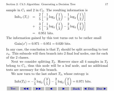
sample in C1 and 2 in C2. The resulting information is
Infox′(T1) =25
[−1
2log2
(12
)− 1
2log2
(12
)]+
35
[−1
3log2
(13
)− 2
3log2
(23
)]= 0.951 bits.
The information gained by this test turns out to be rather small
Gain(x′) = 0.971− 0.951 = 0.020 bits.
In any case, the conclusion is that T1 should be split according to testx4. This subnode will then branch into 2 final leaf nodes, one for eachof the 2 classes.
Next we consider splitting T2. However since all 4 samples in T2
belong to C1, thus this node will be a leaf node, and no additionaltests are necessary for this branch.
We now turn to the last subset T3, whose entropy is
Info(T3) = −35
log2
(35
)− 2
5log2
(25
)= 0.971 bits.
Toc JJ II J I Back J Doc Doc I
Section 2: C4.5 Algorithm: Generating a Decision Tree 18
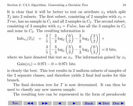
It is clear that it will be better to test on attribute x3 which splitT2 into 2 subsets. The first subset, consisting of 2 samples with x3 =True, has no sample in C1 and all 2 samples in C2. The second subset,consisting of 3 samples with x3 = False, has all the 3 samples in C1
and none in C2. The resulting information is
Infox5(T3) =25
[−2
2log2
(02
)− 2
2log2
(22
)]+
35
[−3
3log2
(33
)− 0
3log2
(03
)]= 0 bits,
where we have denoted this test as x5. The information gained by x5
Gain(x5) = 0.971− 0 = 0.971 bits
is clearly the best. This test results in 2 uniform subsets of samples ofthe 2 separate classes, and therefore yields 2 final leaf nodes for thisbranch.
The final decision tree for T is now determined. It can then beused to classify any new unseen sample.
The resulting tree can be represented in the form of pseudocode
Toc JJ II J I Back J Doc Doc I
Section 2: C4.5 Algorithm: Generating a Decision Tree 19
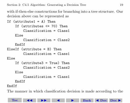
with if-then-else constructions for branching into a tree structure. Ourdecision above can be represented asIf (attribute1 = A) Then
If (attributes <= 70) ThenClassification = Class1
ElseClassification = Class2
EndIfElseIf (attribute = B) Then
Classification = Class1Else
If (attribute3 = True) ThenClassification = Class2
ElseClassification = Class1
EndIfEndIf
The manner in which classification decision is made according to the
Toc JJ II J I Back J Doc Doc I
Section 2: C4.5 Algorithm: Generating a Decision Tree 20
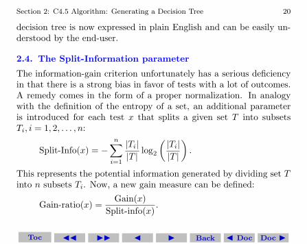
decision tree is now expressed in plain English and can be easily un-derstood by the end-user.
2.4. The Split-Information parameter
The information-gain criterion unfortunately has a serious deficiencyin that there is a strong bias in favor of tests with a lot of outcomes.A remedy comes in the form of a proper normalization. In analogywith the definition of the entropy of a set, an additional parameteris introduced for each test x that splits a given set T into subsetsTi, i = 1, 2, . . . , n:
Split-Info(x) = −n∑
i=1
|Ti||T |
log2
(|Ti||T |
).
This represents the potential information generated by dividing set Tinto n subsets Ti. Now, a new gain measure can be defined:
Gain-ratio(x) =Gain(x)
Split-info(x).
Toc JJ II J I Back J Doc Doc I
Section 2: C4.5 Algorithm: Generating a Decision Tree 21
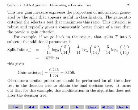
This new gain measure expresses the proportion of information gener-ated by the split that appears useful in classification. The gain-ratiocriterion the selects a test that maximizes this ratio. This criterion isrobust and typically gives a consistently better choice of a test thanthe previous gain criterion.
For example, if we go back to the test x1 that splits T into 3subsets, the additional parameter is
Split-Info(x1) = − 514
log2
(514
)− 4
14log2
(414
)− 5
14log2
(514
)= 1.577bits
this gives
Gain-ratio(x1) =0.2461.557
= 0.156.
Of course a similar procedure should be performed for all the othertest in the decision tree to obtain the final decision tree. It turnsout that for this example, this modification in the algorithm does notalter the decision tree.
Toc JJ II J I Back J Doc Doc I
Section 2: C4.5 Algorithm: Generating a Decision Tree 22
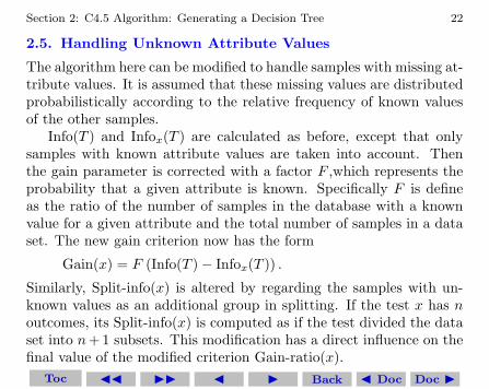
2.5. Handling Unknown Attribute Values
The algorithm here can be modified to handle samples with missing at-tribute values. It is assumed that these missing values are distributedprobabilistically according to the relative frequency of known valuesof the other samples.
Info(T ) and Infox(T ) are calculated as before, except that onlysamples with known attribute values are taken into account. Thenthe gain parameter is corrected with a factor F ,which represents theprobability that a given attribute is known. Specifically F is defineas the ratio of the number of samples in the database with a knownvalue for a given attribute and the total number of samples in a dataset. The new gain criterion now has the form
Gain(x) = F (Info(T )− Infox(T )) .
Similarly, Split-info(x) is altered by regarding the samples with un-known values as an additional group in splitting. If the test x has noutcomes, its Split-info(x) is computed as if the test divided the dataset into n + 1 subsets. This modification has a direct influence on thefinal value of the modified criterion Gain-ratio(x).
Toc JJ II J I Back J Doc Doc I
Section 2: C4.5 Algorithm: Generating a Decision Tree 23
2.6. Pruning Decision Trees
Generating a decision to function best with a given of training dataset often creates a tree that over-fits the data and is too sensitive onthe sample noise. Such decision trees do not perform well with newunseen samples.
We need to prune the tree in such a way to reduce the predictionerror rate. Pruning a decision tree means that one or more subtreesare discarded and replaced with leaves thus simplifying the tree. Onepossibility to estimate the prediction error rate is to use the cross-validation techniques. This technique divides initially available sam-ples into roughly equal-sized blocks and, for each block, the tree isconstructed from all sample except this block and tested with thatblock of samples. With the available training and testing samples,the basic idea is to remove parts of the tree that do not contributeto the classification accuracy of unseen testing samples. producing aless complex and thus more comprehensible tree.
Toc JJ II J I Back J Doc Doc I
Section 2: C4.5 Algorithm: Generating a Decision Tree 24
2.7. Advantages and disadvantages
Decision trees in general has several important advantages:
1. creating decision trees need no tuning parameters
2. no assumptions about distribution of attribute values or inde-pendence of attributes
3. no need for transformation of variables (any monotonic trans-formation of the variable will result in the same trees)
4. the method automatically finds a subset of the features that arerelevant to the classification
5. decision trees are robust to outliers as the choices of a splitdepends on the ordering of feature values and not on the absolutemagnitudes of these values
6. it can easily be extended to handle samples with missing values
Decision trees also has several important disadvantages:
1. If data samples are represented graphically in an n-dimensionalspace, then a decision tree divides the space into regions. each
Toc JJ II J I Back J Doc Doc I
Section 2: C4.5 Algorithm: Generating a Decision Tree 25
region is labeled with a corresponding class. An unseen sam-ple is classified by determining the region in which the givenlies. Decision tree is constructed by successive refinement, split-ting existing regions into smaller ones that contain highly con-centrated points of one class. The number of training samplesneeded to construct a good classifier is proportional to the num-ber of regions.
2. Decision rules yield orthogonal hyperplanes in the n-dimensionalspace, thus each region has the form of a hyper-rectangle. Butif in reality many of these decision hyperplanes are not perpen-dicular to the coordinates (because certain deciding factors arethe results of combinations of different attributes), decision treesand rules tend to be much more complex. Of course a solutionis to better transform the data in the pre-processing step.
3. There is a type of classification problem where the classificationcriterion has the form: a given class is supported if n out of mconditions are present. Decision trees are not the appropriatetool for modeling this type of problems. Medical diagnostic
Toc JJ II J I Back J Doc Doc I
Section 2: C4.5 Algorithm: Generating a Decision Tree 26
decisions are a typical example of this kind of classification. If4 out of 11 symptoms support diagnosis of a given disease, thenthe corresponding classifier will generate 330 regions in an 11-dimensional space for positive diagnosis only. That correspondsto 330 decision rules.
References
[1] M. Kantardzic, Data Mining - Concepts, Models, Methods, andAlgorithms, IEEE Press, Wiley-Interscience, 2003, ISBN 0-471-22852-4. This is our adopted textbook, from which this set oflecture notes are derived primarily.
[2] J. R. Quinlan, C4.5: Programs for Machine Learning, MorganKaufmann Publishers, 1993.
[3] J. R. Quinlan, ”Improved use of continuous attributes in c4.5”,Journal of Artificial Intelligence Research, 4:77-90, 1996.
[4] Computationally there is actually no need to know the informationcontent before performing any test to attempt to split the samples
Toc JJ II J I Back J Doc Doc I
Section 2: C4.5 Algorithm: Generating a Decision Tree 27
in a group. Finding a test x that maximizes
Gain(x) = Info(T )− Infox(T )
is the same as finding a test x that minimizes Infox(T ).
11
Toc JJ II J I Back J Doc Doc I