Decision uncertainty in multiobjective optimization

Preprint No. M 16/06

Gabriele Eichfelder, Corinna Krüger and Anita Schöbel

August 2016

Impressum: Hrsg.: Leiter des Instituts für Mathematik

Weimarer Straße 25 98693 Ilmenau

Tel.: +49 3677 69-3621 Fax: +49 3677 69-3270 http://www.tu-ilmenau.de/math/

Technische Universität Ilmenau Institut für Mathematik

Decision Uncertainty in Multiobjective Optimization

Gabriele Eichfelder1, Corinna Kruger∗2, and Anita Schobel2

1Institute for Mathematics, Technische Universitat Ilmenau,Po 10 05 65, 98684 Ilmenau, Germany

2Institute for Numerical and Applied Mathematics, University of Gottingen,Lotzestr. 16-18, 37083 Gottingen, Germany

August 16, 2016

Abstract

In many real-world optimization problems, a solution cannot be realized in practiceexactly as computed, e.g., it may be impossible to produce a board of exactly 3.546 mmwidth. Whenever computed solutions are not realized exactly but in a perturbed way,we speak of decision uncertainty. We study decision uncertainty in multiobjective opti-mization problems and we propose the concept decision robust efficiency for evaluatingthe robustness of a solution in this case. Therefore, we address decision uncertaintywithin the framework of set-valued maps. First, we prove that convexity and continuityare preserved by the resulting set-valued mappings. Second, we obtain specific resultsfor particular classes of objective functions that are relevant for solving the set-valuedproblem. We furthermore prove that decision robust efficient solutions can be found bysolving a deterministic problem in case of linear objective functions. We also investigatethe relationship of the proposed concept to other concepts in the literature.

1 Introduction

When applying mathematical optimization methods to real world problems, several difficul-ties have to be considered. We study a class of problems where two specific difficulties occursimultaneously. First, the problem can have several conflicting objectives, leading to a mul-tiobjective optimization problem. Secondly, a calculated solution may only be realized withinsome accuracy instead of being put into practice exactly. Realizations of calculated solutionshave to be considered uncertain in this case. In the following, we refer to this kind of uncer-tainty as decision uncertainty since the decision variables are the source of uncertainty insidethe problem. We distinguish decision uncertainty from parameter uncertainty in optimizationproblems, see, e.g., [BTGN09], where the values of parameters are not known at the time aproblem is solved.

In recent years, multiobjective optimization problems including parameter uncertainty havebeen studied in various ways. In [KL12] and [GJLVP14], the authors consider for each solutionthe vector consisting in each component of the worst case of the corresponding objective in

∗Supported by DFG RTG 1703 “Resource Efficiency in Corporate Networks”

1

place of the uncertain objective. [EIS14] and [AB08] compare solutions by the sets of theirpossible outcome vectors. Solutions that are effficient for all realizations of uncertainty arestudied, e.g., in [GLP13]. For a survey of different concepts of robustness in the literature,we refer the reader to [IS16].

Single-objective optimization problems including decision uncertainty have been treated withminmax robustness for instance in [Das97], [LP09] and [BS07]. Decision uncertainty in multi-objective optimization has been addressed by evaluating the mean or integral of each objectiveover the set of possible values of a solution, see, e.g. [DG06], or by sensitivity analysis, see,e.g., [BA06]. However, until now, there exists no worst-case robustness approach for decisionuncertainty in multiobjective optimization.

In this work, we investigate decision uncertainty in multiobjective optimization with a minmaxrobustness approach based on set-valued optimization, i.e., we define and analyze a robustcounterpart for this kind of problem and we present approaches for solving it.The conceptual idea of the presented robustness concept, which we call decision robust effi-ciency, is based on a minmax robustness approach for parameter uncertainty in multiobjectiveoptimization introduced by [EIS14]. However, exploiting the specific structure arising in prob-lems with decision uncertainty, we obtain results that are generally not valid for problemswith parameter uncertainty.

In the following paragraphs we sketch practical applications of multiobjective problems thatare affected by decision uncertainty. Definitions from set-valued optimization are recalled inSection 2. Following on that, the robustness concept decision robust efficiency is developed.In Section 3, the set-valued functions that correspond to decision robust efficiency are inves-tigated with respect to continuity and convexity properties. Section 4 relates the presentedrobustness concept to approaches in the literature. Solution approaches for problem classeswith specific objective functions are studied in Section 5.

Applications

We present two real-world applications for multiobjective decision uncertainty. First, wepresent an application in the Lorentz force velocimetry framework and secondly, we presentthe Growing Media Mixing Problem for plant nurseries. Both applications can be modeledas biobjective optimization problems with decision uncertainty.

Lorentz Force Velocimetry (LFV) Framework The LFV is an electromagnetic non-contact flow measurement technique for electrically conducting fluids. This is especially suitedfor corrosive or extremely hot fluids like glass melts or acidic mixtures which can damageother measurement setups [DTE14]. The magnetic field of the permanent magnets interactswith an electrically conducting fluid which moves through a channel, see Figure 1. Eddy

Figure 1: Illustration of a non-contact flow measurement system with 8 magnets.

2

currents develop and the resulting secondary magnetic field acts on the magnet system. TheLorentz force breaks the fluid and an equal but opposite force deflects the magnet system,which can be measured. Fluids with a small electrical conductivity produce only very smallLorentz forces. Thus, a sensitive balance system is required for a reliable measurement. Thislimits the weight of the external magnet system. Therefore, we obtain two conflicting goals:maximize the Lorentz force and minimize the magnetization. As variables, the direction ofthe magnetization of each magnet and the magnetization have to be optimized.Figure 1 gives a simple arrangement of eight permanent magnets around a channel. Inpractice an (optimally) chosen magnetic direction cannot be realized in the desired accuracy,as magnets can only be produced with a guarantee of the magnetic directions within sometolerance interval. Therefore, decision uncertainty has to be taken into account here, in orderto avoid solutions with practical realizations that are far from being efficient in the worstcase.

Growing Media Mixing Problem for a Plant Nursery For each plant species, a plantnursery that produces potted plants has to decide the type of planter pot and the type ofgrowing media to be used. First, possible types of planter pots are plastic pots made fromfossil ressources and bio-degradable planter pots. The former are cheaper, while the latterare more eco-friendly. Secondly, the growing media can be chosen as a mixture of peat andcompost, where the feasible mixing ratio lies between 100% peat and 33% peat plus 66%compost. The corresponding decision problem consists of determining one type of planter potand one mixing ratio for each plant species such that two objectives, i.e., costs and globalwarming potential, are minimized.However, a chosen mixing ratio can usually not be put into practice exactly. Workers in plantnurseries are used to work rather fast than exactly and the different types of soil are oftenmixed in a rough fashion only. Hence, the mixing ratio will vary in each planter pot. Becausethe mixing ratio influences the quality of the raised plant and therefore its selling price,decision uncertainty has to be taken into account in this biobjective optimization problem.A detailed study of this problem can be found in [CKGS16].

2 Decision Robust Efficiency

We consider the (deterministic) multiobjective optimization problem

(P) minx∈Ω

f(x)

with feasible set Ω ⊆ Rn and objective function f : Ω → Rk. We want to take into accountthe fact that the decision variables in (P) are uncertain, i.e., they can not be realized exactlyas computed.The practical realization of a solution x ∈ Rn is composed of x and a perturbation from afixed perturbation set Z ⊆ Rn, i.e., the realization of a solution x is an element of the setx+ Z = x + z | z ∈ Z. Because a solution might as well be put into practice exactly asplanned, we require 0 ∈ Z. Decision uncertainty in (P) is modeled by considering the familyof optimization problems (

P(z) minx+z∈Ω

f(x+ z), z ∈ Z).

3

The goal is to find a solution x without knowing the value of the perturbation z. We wantto hedge against the worst case. Addressing decision uncertainty within the framework ofrobust optimization, we define:

Definition 1. A point x ∈ Rn is called decision robust feasible for (P(z), z ∈ Z) if x+ z |z ∈ Z ⊆ Ω, i.e., if all realizations of x are feasible solutions. We call

X := x ∈ Rn | x+ z ∈ Ω for all z ∈ Z

the set of decision robust feasible solutions.

Definition 1 takes a conservative point of view since x is required to be feasible for everyperturbation that may occur. This conceptual idea corresponds to strict robust feasibility by[BTGN09] for single-objective robust optimization with parameter uncertainty.

In the remainder of the paper, we make the following two assumptions:

• We assume Z ⊆ Rn is a compact set and 0 ∈ Z. Hence, X ⊆ Ω.

• We furthermore assume X 6= ∅.

For each decision robust feasible solution x ∈ X we define the image set of all realizations ofx as

fZ(x) := f(x+ z) | z ∈ Z.

In order to develop a solution concept for (P(z), z ∈ Z), we recall solution concepts fromboth, multiobjective optimization and set-valued optimization.

2.1 Approach using Multiobjective Optimization

In the following, we write cl(·), int (·) and bd(·) for the closure, the interior and the boundaryof a set, respectively. Furthermore, we denote the open and closed ball of radius ε > 0 fora given norm ‖ · ‖ on Rk around a point y ∈ Rk as B(y, ε) := y ∈ Rk | ‖y‖ < ε andB(y, ε) := y ∈ Rk | ‖y‖ ≤ ε.Recall that a nonempty set K is called a cone if λk ∈ K for all λ ≥ 0 and all k ∈ K, pointedif K ∩ (−K) = 0, and solid if int (K) 6= ∅. A cone K is convex if and only if K +K = K.It is well known that for a convex pointed cone K we have K + int (K) = int (K) as well asK\0 + K = K\0 and that the sets int (K) and K\0 are also convex (see for instance[Jah11]). A closed convex pointed and solid cone K ⊆ Rk defines a partial order on Rk. Weconsider the following relations:

x [</≤/5] y ⇔ y − x ∈ [int(K)/K\0/K]

A possible choice for K ⊆ Rk is K = Rk+ :=y ∈ Rk | yi ≥ 0, ∀1 ≤ i ≤ k

. Then the partial

order introduced by K is also called the component-wise or natural order on Rk.Given a closed, convex, pointed and solid cone K ⊆ Rk, the classical optimality concepts forthe deterministic multiobjective problem (P) are given in the following definition. We remarkthat efficiency is often refered to as (Edgeworth-) Pareto minimality.

Definition 2. A solution x∗ ∈ Ω is called [weakly/·/strictly] efficient for (P) if there is nox ∈ Ω \ x∗ with the property f(x) ∈ f(x∗) − [int(K)/K\0/K].

4

In order define a concept for a solution of the decision uncertain problem (P(z), z ∈ Z), wereplace the outcome vector f(x) in Definition 2 by the set fZ(x).

Definition 3. A solution x∗ ∈ X is called a decision robust [weakly/·/strictly] efficientsolution of (P(z), z ∈ Z), if there is no x ∈ X\x∗ with the property

fZ(x) ⊆ fZ(x∗)− [int(K)/K\0/K]. (1)

Therefore, by decision robust efficiency, we obtain a solution concept for the decision uncertainmultiobjecive problem (P(z), z ∈ Z).

2.2 Approach using Set-Valued Optimization

Considering the image set of all realizations fZ(x) for all x ∈ X defines a set-valued mapfZ : X ⇒ Rk. We define the Robust Counterpart (RC) of the decision uncertain multiobjectiveproblem (P(z), z ∈ Z) as the set-valued optimization problem

(RC) minx∈X

fZ(x).

Next, we see that the decision robust efficient solutions of (P(z), z ∈ Z) are exactly the optimalsolutions to the set-valued problem (RC). In set-valued optimization, i.e., in optimization witha set-valued objective function, the so called set approach [EJ12, HJ11, Kur98] uses orderrelations to compare the sets that are the images of the objective function. One widely usedorder relation is the u-type less order relation 4K , see [HJ11, Def. 3.2], which is defined forarbitrary nonempty sets A,B ⊆ Rk by

A 4K B :⇔ A ⊆ B −K. (2)

The order relation 4K is a reflexive and transitive binary relation. It can also be written inthe following form:

A 4K B ⇔ (∀a ∈ A ∃b ∈ B : a 5 b). (3)

If we replace K by K\0 or int (K) in (2), and thus 5 by ≤ or by < in (3), we analogouslyobtain the set relations 4K\0 and 4int(K) . However, these are no longer reflexive.

In order to specify optimal solutions of the set-valued optimization problem (RC), we makeuse of the following definition, see, e.g., [RMS07].

Definition 4. Let a nonempty set X ⊆ Rn and a set-valued map H : X ⇒ Rk be givenwith H(x) 6= ∅ for all x ∈ X. The element x∗ ∈ X is called strictly optimal solution of theset-valued optimization problem

minx∈X

H(x)

w.r.t. 4, where 4∈ 4K ,4int(K),4K\0, if there exists no x ∈ X\x∗ with H(x) 4 H(x∗).

Using the set relation (2) we can replace

fZ(x) ⊆ fZ(x∗)− [int(K)/K\0/K]

in (1) byfZ(x) [4int(K) /4K\0 /4K ] fZ(x∗)

as done similarly in [IKK+14] for multi-objective parameter uncertainty. Consequently, wereceive equivalence of the optimal solutions to (RC) using Definition 4 and regularizationrobust efficient solutions according to Definition 3.

5

Proposition 5. The point x∗ ∈ X is a decision robust [weakly/·/strictly] efficient solution of(P(z), z ∈ Z) if and only if x∗ ∈ X is a strictly optimal solution of the set-valued optimizationproblem (RC) w.r.t. [4int(K) /4K\0 /4K ].

The following example illustrates decision robust efficiency. It shows that decision robustefficient solutions are not necessarily efficient for the deterministic problem (P).

Example 6. Let

(P) minx∈Ω

(x21−x2

)and

(P(z), z ∈ Z) =

(minx+z∈Ω

((x1+z1)2

−x2−z2

), z ∈ Z

),

where

Ω = conv(−0.6

0

),(−0.6

1

), ( 1

1 ) , ( 10 ) ,(

0.7−0.3

),(−0.3−0.3

)and Z = conv

((−0.60

), ( 0

0 ) ,(−0.3−0.3

)).

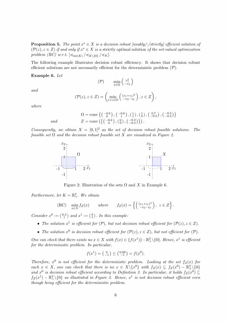
Consequently, we obtain X = [0, 1]2 as the set of decision robust feasible solutions. Thefeasible set Ω and the decision robust feasible set X are visualized in Figure 2.

x1

x2

-1 1 2

-1

1

2

Ω

x1

x2

-1 1 2

-1

1

2

X

Figure 2: Illustration of the sets Ω and X in Example 6.

Furthermore, let K = R2+. We obtain

(RC) minx∈X

fZ(x) where fZ(x) =(

(x1+z1)2

−x2−z2

), z ∈ Z

.

Consider x0 := ( 0.31 ) and x1 := ( 0

1 ) . In this example:

• The solution x1 is efficient for (P), but not decision robust efficient for (P(z), z ∈ Z).

• The solution x0 is decision robust efficient for (P(z), z ∈ Z), but not efficient for (P).

One can check that there exists no x ∈ X with f(x) ∈ f(x1)−R2+\0. Hence, x1 is efficient

for the deterministic problem. In particular,

f(x1) =(

0−1

)≤(

0.09−1

)= f(x0).

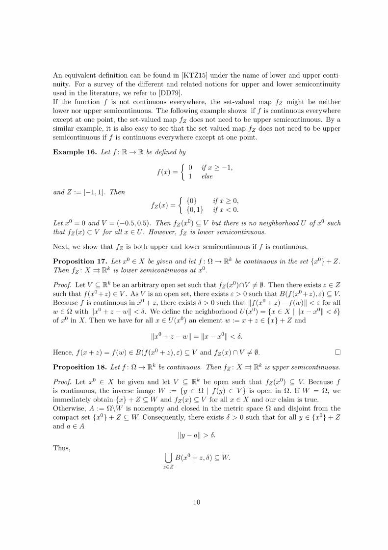
Therefore, x0 is not efficient for the deterministic problem. Looking at the set fZ(x) foreach x ∈ X, one can check that there is no x ∈ X\x0 with fZ(x) ⊆ fZ(x0) − R2

+\0and x0 is decision robust efficient according to Definition 3. In particular, it holds fZ(x0) ⊆fZ(x1) − R2

+\0 as illustrated in Figure 3. Hence, x1 is not decision robust efficient eventhough being efficient for the deterministic problem.

6

f1(x)

f2(x)

(0,-0.5)

fZ(x1)

fZ(x0)

f1(x)

f2(x)

fZ(x1)− R2+\0

fZ(x0)

Figure 3: Relationship of the set fZ(x0) and the set fZ(x1) in Example 6.

2.3 Approach using Supremal Sets

In minmax robust optimization, solutions are determined that perform best in the objectivefunction when evaluated together with worst-case realizations of uncertainty. Therefore, weinvestigate suprema of the sets fZ(x) for x ∈ X. We show that minimizing the supremal setsof the sets fZ is equivalent to solving (RC).We use a concept for the supremum of a set that is defined and studied thoroughly in [Nie80]and [Loh11].

Definition 7. For a bounded nonempty subset A ( Rk the supremal set of A is defined as

Sup(A) = y ∈ cl(A−K) | (y+ int (K)) ∩ cl (A−K) = ∅.

According to [Loh11, Cor. 1.48, Cor. 1.49], for a bounded nonempty subset A ( Rk it holds

Sup(A) = bd (Sup(A)−K). (4)

For an illustration of a supremal set, we refer to Figure 3. The boundary of the blue set, iclud-ing the broken and unbrocken blue lines, is exactly the supremal set of fZ(x1) in Example 6.Following Definition 7, we formulate another set-valued optimization problem

minx∈X

fSup(x) with fSup : X ⇒ Rk, x 7→ Sup (fZ(x)). (5)

In general set-valued optimization problems, the image set of the objective function, suchas fSup(x) in (5), is assumed to be nonempty. Therefore, we additionally assume f to becontinuous in the remainder of the section.

Remark 8. Due to our assumptions, the perturbation set Z is nonempty and compact andf : Ω→ Rk is continuous. Hence, fZ(x) is compact and nonempty for all x ∈ X ⊆ Ω and

fZ(x)−K = cl (fZ(x)−K) 6∈ Rk, ∅.

According to Corollary 1.44 in [Loh11], this directly implies

fSup(x) = Sup(fZ(x)) 6= ∅.

The following lemma is fundamental for our main result which relates the solutions of (5) to thesolutions of (RC) and the decision robust [weakly/·/strictly] efficient solutions of (P(z), z ∈Z).

7

Lemma 9. Let A,B ( Rk be compact sets. Then

A− [int(K)/K\0/K] = Sup (A)− [int(K)/K\0/K]

and thus for any 4∈ 4K ,4int(K),4K\0 it holds

A 4 B ⇔ Sup (A) 4 Sup (B).

Proof. In [Loh11, Chapter 1] it was shown that Sup (A)−int (K) = cl(A−K)−int (K). As A iscompact andK is closed we have cl(A−K) = A−K and we get Sup (A)−int (K) = A−int (K).Next we show

A−K = Sup (A)−K. (6)

By [Loh11] we have cl (A−K) = Sup (A) ∪ (Sup (A)− int (K)). And thus

A−K = cl (A−K) = Sup (A) ∪ (Sup (A)− int (K)) ⊆ Sup (A)−K.

By the definition of the supremal set and the compactness of A we also have Sup (A)−K ⊆cl (A−K)−K = A−K and we have shown (6). Finally we get from (6)

A−K\0 = A−K −K\0 = Sup (A)−K −K\0 = Sup (A)−K\0.

Due to Relation (2) we obtain the last assertion:

A ⊆ B − [int(K)/K\0/K] ⇔ A−K ⊆ B − [int(K)/K\0/K]⇔ Sup (A)−K ⊆ Sup (B)− [int(K)/K\0/K]⇔ Sup (A) ⊆ Sup (B)− [int(K)/K\0/K].

Due to Z being compact, the set fZ(x) is compact for a continuous objective function f andfor each x ∈ X.

Corollary 10. Let f be continuous. Then it holds for all x, x′ ∈ X and 4∈ 4K ,4int(K),4K\0

fZ(x) 4 fZ(x′) if and only if Sup (fZ(x)) 4 Sup(fZ(x′)

),

i.e., the set-valued optimization problems (RC) and (5) are equivalent in the sense that thesets of strictly optimal solutions w.r.t. [4int(K) /4K\0 /4K ] are the same.

Using Proposition 5 and Corollary 10 we directly obtain our main result of this section.

Theorem 11. Let f be continuous. The point x∗ ∈ X is a decision robust [weakly/·/strictly]efficient solution of (P(z), z ∈ Z) if and only if x∗ ∈ X is a strictly optimal solution for theset-valued optimization problem (5) w.r.t. [4int(K) /4K\0 /4K ].

3 Properties of the Set-Valued Functions fZ(·) and Sup(fZ(·))We prove that convexity of the vector-valued function f implies convexity of the set-valuedmapping fZ . Furthermore, we prove that continuity of the vector-valued function f is pre-served when considering the set-valued mapping fZ or the respective supremal sets of itsimages instead of f.

8

3.1 Convexity

We start by recalling the definition of a K-convex single-valued and a K-convex set-valuedmap for a convex cone K. See here, e.g., [Kur96, Def. 2.1],[AF90, Lemma 2.1.2] as well as[BP03] and the references therein.

Definition 12. Let Y ⊆ Rn be a convex set. A map f : Y → Rk is called K-convex, if for allx1, x2 ∈ Y and λ ∈ [0, 1] it holds that λf(x1) + (1− λ)f(x2) ∈ f(λx1 + (1− λ)x2)+K.

Definition 13. Let Y ⊆ Rn be a convex set. A set-valued map H : Y ⇒ Rk is called K-convex,if for all x1, x2 ∈ Y and λ ∈ [0, 1] it holds that λH(x1)+(1−λ)H(x2) ⊆ H(λx1+(1−λ)x2)+K.

Proposition 14. Let Ω and Z be convex. Let f : Ω→ Rk be a K-convex single-valued map.Then, X is a convex set and fZ : X ⇒ Rk is a K-convex set-valued map.

Proof. For fixed z ∈ Z, the set x ∈ Rn | x + z ∈ Ω is convex. Hence, X =⋂z∈Zx ∈ Rn |

x+ z ∈ Ω is convex as an intersection of convex sets.Let a ∈ fZ(x1) and b ∈ fZ(x2) be arbitrarily chosen. Then there exist z1, z2 ∈ Z witha = f(x1 + z1) and b = f(x2 + z2). With x := λx1 + (1−λ)x2 and z := λ z1 + (1−λ) z2 ∈ Zwe obtain

λ a+ (1− λ) b = λ f(x1 + z1) + (1− λ) f(x2 + z2)∈ f(λ (x1 + z1) + (1− λ) (x2 + z2))+K= f(x+ z)+K⊆ fZ(x) +K.

Note that Sup(fZ(·)) is not a K-convex map and that, in contrast to K-convexity, linearityof a function f : Ω→ Rk does not necessarily lead to linearity in the corresponding set-valuedfunction fZ : X ⇒ Rk.

3.2 Semicontinuity

We prove that, if f is continuous everywhere, the set-valued functions fZ and Sup(fZ(·))inherit continuity properties. We show that continuity of f leads to semicontinuity of fZ .Moreover, Sup(fZ(·)) is lower but not necessarily upper semicontinuous if f is continuous.

Throughout this section, we consider the feasible set Ω ⊆ Rn as a metric space. Ω is equippedwith the metric derived from an arbitrary norm ‖ · ‖ on Rn. Hence, we can use the followingdefinition of [AF90, Section 1.4] to define semicontinuity on subsets of Rn, such as Ω.

Definition 15. Let S be a metric space and let H : S ⇒ Rk be a set-valued map.

(a) H is called lower semicontinuous at x0 ∈ S, if for all open sets V ⊆ Rk with H(x0)∩V 6=∅ there is a neighborhood U of x0 such that H(x) ∩ V 6= ∅ for all x ∈ U . H is lowersemicontinuous if it is lower semicontinuous at any x0 ∈ S.

(b) H is called upper semicontinuous at x0 ∈ S if for all open sets V ⊆ Rk with H(x0) ⊆ Vthere is a neighborhood U of x0 such that H(x) ⊆ V for all x ∈ U . H is uppersemicontinuous if it is upper semicontinuous at any x0 ∈ S.

9

An equivalent definition can be found in [KTZ15] under the name of lower and upper conti-nuity. For a survey of the different and related notions for upper and lower semicontinuityused in the literature, we refer to [DD79].If the function f is not continuous everywhere, the set-valued map fZ might be neitherlower nor upper semicontinuous. The following example shows: if f is continuous everywhereexcept at one point, the set-valued map fZ does not need to be upper semicontinuous. By asimilar example, it is also easy to see that the set-valued map fZ does not need to be uppersemicontinuous if f is continuous everywhere except at one point.

Example 16. Let f : R→ R be defined by

f(x) =

0 if x ≥ −1,1 else

and Z := [−1, 1]. Then

fZ(x) =

0 if x ≥ 0,0, 1 if x < 0.

Let x0 = 0 and V = (−0.5, 0.5). Then fZ(x0) ⊆ V but there is no neighborhood U of x0 suchthat fZ(x) ⊂ V for all x ∈ U . However, fZ is lower semicontinuous.

Next, we show that fZ is both upper and lower semicontinuous if f is continuous.

Proposition 17. Let x0 ∈ X be given and let f : Ω→ Rk be continuous in the set x0+Z.Then fZ : X ⇒ Rk is lower semicontinuous at x0.

Proof. Let V ⊆ Rk be an arbitrary open set such that fZ(x0)∩V 6= ∅. Then there exists z ∈ Zsuch that f(x0 +z) ∈ V . As V is an open set, there exists ε > 0 such that B(f(x0 +z), ε) ⊆ V.Because f is continuous in x0 + z, there exists δ > 0 such that ‖f(x0 + z)− f(w)‖ < ε for allw ∈ Ω with ‖x0 + z − w‖ < δ. We define the neighborhood U(x0) = x ∈ X | ‖x− x0‖ < δof x0 in X. Then we have for all x ∈ U(x0) an element w := x+ z ∈ x+ Z and

‖x0 + z − w‖ = ‖x− x0‖ < δ.

Hence, f(x+ z) = f(w) ∈ B(f(x0 + z), ε) ⊆ V and fZ(x) ∩ V 6= ∅.

Proposition 18. Let f : Ω→ Rk be continuous. Then fZ : X ⇒ Rk is upper semicontinuous.

Proof. Let x0 ∈ X be given and let V ⊆ Rk be open such that fZ(x0) ⊆ V. Because fis continuous, the inverse image W := y ∈ Ω | f(y) ∈ V is open in Ω. If W = Ω, weimmediately obtain x+ Z ⊆W and fZ(x) ⊆ V for all x ∈ X and our claim is true.Otherwise, A := Ω\W is nonempty and closed in the metric space Ω and disjoint from thecompact set x0 + Z ⊆ W. Consequently, there exists δ > 0 such that for all y ∈ x0 + Zand a ∈ A

‖y − a‖ > δ.

Thus, ⋃z∈Z

B(x0 + z, δ) ⊆W.

10

We define the neighborhood U := B(x0, δ) ⊆ X. For all x ∈ U and z ∈ Z we have ‖x + z −(x0 + z)‖ = ‖x− x0‖ < δ and

x+ Z ⊆⋃z∈Z

B(x0 + z, δ) ⊆W,

where B(x0 + z, δ) denotes an open ball in the metric space Ω for all z ∈ Z. Therefore, for allx ∈ U

fZ(x) ⊆ f(w) | w ∈W ⊆ V.

As we have seen in Theorem 11, determining whether a decision robust feasible solution isdecision robust efficient is equivalent to a comparison of supremal sets. Therefore, we continueby examining semicontinuity properties of the set-valued function

fSup : X ⇒ Rk, x 7→ Sup(fZ(x))

that was already introduced as (5) in Section 2.3.The following lemma serves as a preparation for proving the lower semicontinuity of thefunction fSup in Proposition 20.

Lemma 19. Let ε > 0, and let a ∈ int (K) with ‖a‖ < ε. Then

T = B(0, ε) ∩ (a − int (K)) ∩ (−a+ int (K))

(a) is convex and open,

(b) B(0, ε) ⊆ T ⊆ B(0, ε) for some 0 < ε < ε,

(c) T is symmetric, i.e. T = −T.

(d) For all s, u ∈ Rk it holds

s+ T ⊆ u − int (K) ⇔ u+ T ⊆ s+ int (K).

(e) a ∈ cl (T ).

Proof. The set T is convex and open as an intersection of three convex sets, hence (a) holds.Furthermore, T ⊆ B(0, ε). To see the second part of (b), note that 0 ∈ T because 0 ∈ B(0, ε),0 = a− a ∈ a − int (K) and 0 = −a+ a ∈ −a+ int (K). Because T is open, there existsε > 0 such that B(0, ε) ⊆ T.Next, (c) results from B(0, ε) = −B(0, ε) and from a − int (K) = − (−a+ int (K)),and (d) is a direct consequence of (c). Finally, for (e), note that a ∈ int (B(0, ε)) and thata ∈ int (−a+ int (K)) since a = −a+ 2 · a and a ∈ int (K). Because a is in the interior ofboth sets, every sequence that is convergent to a has a subsequence that converges to a inB(0, ε) ∩ (−a+ int (K)) . Furthermore, a ∈ cl (a − int (K)) and the result follows.

Proposition 20. Let f : Ω → Rk be continuous. Then fSup : X ⇒ Rk with x 7→ Sup(fZ(x))is lower semicontinuous.

11

Proof. Let x0 ∈ X and let V ⊆ Rk be an open set such that Sup(fZ(x0)) ∩ V 6= ∅. Chooses ∈ Sup(fZ(x0)) ∩ V 6= ∅. Due to Lemma 9 we have for all x ∈ X

fZ(x)−K = Sup(fZ(x))−K. (7)

Therefore, there exist z ∈ Z and k ∈ K such that s := f(x0 + z) − k. Furthermore, thereexists ε > 0 such that s+B(0, ε) ⊆ V.Additionally, there exists a convex neighborhood T of 0 ∈ Rk that satisfies the properties ofLemma 19. In accordance with Property (a) of Lemma 19, let a ∈ Rk such that

T = B(0, ε) ∩ (a − int (K)) ∩ (−a+ int (K)) . (8)

According to Property (b) of Lemma 19, s + T is a convex neighborhood of s satisfyings+B(0, ε) ⊆ s+ T ⊆ s+B(0, ε) ⊆ V . Because f is continuous, there exists for ε > 0some δ0 > 0 such that

f(y) ∈ f(x0 + z)+ T for all y ∈ Ω with ‖y − (x0 + z)‖ < δ0. (9)

Furthermore, fZ is upper semicontinuous in x0 due to Proposition 18. Consequently, thereexists δ1 > 0 such that fZ(x) ⊆ fZ(x0) + T for all x ∈ X with ‖x − x0‖ < δ1. We defineδ := minδ0, δ1. The set U := x ∈ X | ‖x − x0‖ < δ is a neighborhood of x0 in X withrespect to the subset topology inherited from Rn.Assume that there exists x ∈ U such that

Sup(fZ(x)) ∩ (s+ T ) = ∅. (10)

Next, we show that this assumption leads to

s+ T ⊆ Sup(fZ(x))−K. (11)

We have ‖x+ z − (x0 + z)‖ < δ ≤ δ0, hence, using (9) and the definition of s, we get

f(x+ z)− k ∈ s+ T.

Together with (7), we obtain

f(x+ z)− k ∈ (s+ T ) ∩ (fZ(x)−K) = (s+ T ) ∩ (Sup(fZ(x))−K) . (12)

By our assumption (10), f(x+z)−k 6∈ Sup(fZ(x)). Next, we assume that (11) does not hold.Then, there exists t ∈ T such that s+ t 6∈ Sup(fZ(x))−K. Due to (12) and because of s+Tbeing convex due to Lemma 19, there exists w ∈ convf(x + z) − k, s + t such that, using(4),

w ∈ bd (Sup(fZ(x))−K) ∩ (s+ T ) = Sup(fZ(x)) ∩ (s+ T )

in contradiction to assumption (10). Hence, (11) holds and by using (7) and Remark 8 weobtain

cl (s+ T ) ⊆ cl (Sup(fZ(x))−K) = cl (fZ(x)−K) = fZ(x)−K.

By Property (e) in Lemma 19 we get

s+ a ∈ cl (s+ T ) ⊆ fZ(x)−K.

12

Therefore, there exists z ∈ Z such that s+ a ∈ f(x+ z) −K. Consequently, due to (8),

s+ T ⊆ s+ a − int (K) ⊆ f(x+ z) − int (K).

According to Property (d) in Lemma 19 this is equivalent to

f(x+ z)+ T ⊆ s+ int (K).

Because of ‖x− x0‖ < δ ≤ δ1, there exists z0 ∈ Z such that f(x0 + z0) ∈ f(x+ z)+ T. Asa consequence, we finally obtain

f(x0 + z0) ∈ f(x+ z)+ T ⊆ s+ int (K)

in contradiction to s ∈ Sup(fZ(x0)). Thus, (10) does not hold and we have for all x ∈ U

∅ 6= Sup(fZ(x)) ∩ (s+ T ) ⊆ Sup(fZ(x)) ∩ (s+B(0, ε)) ⊆ Sup(fZ(x)) ∩ V.

While the set-valued function fSup(·) = Sup(fZ(·)) is lower semicontinuous, it is not uppersemicontinuous as the following counterexample shows.

Example 21. Let Ω = [−1, 1]2, Z = 0, K = R2+ and f = id: R2 → R2, x 7→ x. Then

X = Ω and we have for all x ∈ X

Sup(fZ(x)) = x − bd(R2+).

The set

V :=z ∈ R2 | z1 ≤ 0

∪z ∈ R2 | z1 > 0, z2 > −

1

z1

is a neighborhood of Sup(fZ(x0)) with x0 = (0, 0)>. We show that for each δ > 0 there existsx ∈ X with ‖x0 − x‖∞ < δ and with Sup(fZ(x)) 6⊆ V . Choose an arbitrary δ > 0 with δ < 2.Then x′ := δ

2(1, 0)> ∈ X satisfies ‖x0 − x′‖∞ < δ. We have w := (δ/2,−4/δ)> ∈ Sup(fZ(x′))but due to

w2 = −4

δ≤ −2

δ= − 1

w1

it holds w 6∈ V . Because δ > 0 can be chosen arbitrarily small, we see that Sup(fZ(·)) is notupper semicontinuous.

The results on the semicontinuity of the functions considered in this section are summarizedin the following table. For continuous objective functions f we have:

fZ(·) Sup(fZ(·))lower semicontinuous 3 3

upper semicontinuous 3 7

Even though Sup(fZ(·)) is not upper semicontinuous, we finally show that Sup(fZ(x0)) andSup(fZ(x)) are arbitrary close for x0, x ∈ X with ‖x0−x‖ < δ if we chose δ > 0 small enough.

13

Theorem 22. Let f : Ω → Rk be continuous. Then for each x0 ∈ X and ε > 0 there existsδ > 0 such that

Sup(fZ(x)) ⊆ Sup(fZ(x0)) +B(0, ε)

for all x ∈ X with ‖x0 − x‖ < δ.

Proof. Let ε > 0 and x0 ∈ X.Due to Lemma 19, there exists a convex neighborhood T of 0 ∈ Rk that satisfies the propertiesof Lemma 19. In accordance with of Lemma 19, let a ∈ Rk such that

T = B(0, ε) ∩ (a − int (K)) ∩ (−a+ int (K)) . (13)

According to Property (b) of Lemma 19, for every v ∈ Rk the set v + T is a convexneighborhood of v satisfying v+ T ⊆ B(v, ε).Because fZ(x0) is compact in Rk and

⋃z∈Zf(x0 + z)+ 1

2T is an open cover of fZ(x0), thereexists a finite subcover

fZ(x0) ⊆⋃z∈Z

f(x0 + z)+1

2T,

which will be indexed by Z ⊆ Z with |Z| <∞. Furthermore, there exists δ1 > 0 such that

fZ(x) ⊆⋃z∈Z

f(x0 + z)+1

2T (14)

for all x ∈ X with ‖x− x0‖ < δ1 because fZ is upper semicontinuous due to Proposition 18.Because f is continuous on Ω, there exists δ(z) > 0 for each z ∈ Z such that

f(y) ∈ f(x0 + z)+1

2T for all y ∈ Ω with ‖y − (x0 + z)‖ < δ(z). (15)

Let δ2 = minδ(z) | z ∈ Z and define δ := minδ1, δ2.We hence have that f(x + z) ∈ f(x0 + z) + 1

2T for all x ∈ X with ‖x0 − x‖ < δ ≤ δ2 and

all z ∈ Z and, because of the symmetry of T due to Property (c) in Lemma 19,

f(x0 + z) ∈ f(x+ z)+1

2T. (16)

Additionally, for each z ∈ Z there exists z ∈ Z such that

f(x0 + z) ∈ f(x0 + z)+1

2T

because our finite subcover is indexed by Z. Together with Relation (16) we see that for eachx ∈ X with ‖x0 − x‖ < δ and z ∈ Z there exists z ∈ Z such that

f(x0 + z) ∈ f(x0 + z)+1

2T ⊆ (f(x+ z)+

1

2T ) +

1

2T = f(x+ z)+ T

because T is convex. Hence, using again the symmetry of T, we obtain for each z ∈ Z theexistence of some z ∈ Z such that

f(x+ z) ∈ f(x0 + z)+ T. (17)

14

In order to prove Theorem 22, we assume on the contrary that there exists x ∈ X with‖x0 − x‖ < δ such that

Sup(fZ(x)) 6⊆ Sup(fZ(x0)) + T. (18)

Then there exists y ∈ Sup(fZ(x)) such that y 6∈ Sup(fZ(x0)) + T and, due to the symmetryof T,

(y+ T ) ∩ Sup(fZ(x0)) = ∅. (19)

Recall from Lemma 9 that for all x′ ∈ X

fZ(x′)−K = Sup(fZ(x′))−K. (20)

From (20) we know that there exist z ∈ Z and k ∈ K such that

y = f(x+ z)− k. (21)

Next, we show that Assumption (19) leads to

y+ T ⊆ Sup(fZ(x0))−K. (22)

We have ‖x− x0‖ < δ ≤ δ1. Due to (14) together with the symmetry of T, there exists z ∈ Zsuch that f(x0 + z) ∈ f(x + z) + 1

2T ⊆ f(x + z) + T, because T is convex and 0 ∈ T.Hence, we get from (21)

f(x0 + z)− k ∈ (y+ T ) ∩(Sup(fZ(x0))−K

). (23)

By assumption (19), f(x0 + z)− k 6∈ Sup(fZ(x0)).We assume that (22) does not hold. Then, there exists t ∈ T such that y+t 6∈ Sup(fZ(x0))−K.Because y+ T is convex and due to (23), there exists

w ∈ convf(x0 + z)− k, y + t ⊆ y+ T

such that, using (4),

w ∈ bd(Sup(fZ(x0))−K

)∩ (y+ T ) = Sup(fZ(x0)) ∩ (y+ T )

in contradiction to (19). Hence, (22) holds and by using (20) we obtain

cl (y+ T ) ⊆ cl(Sup(fZ(x0))−K

)= cl

(fZ(x0)−K

).

By Property (e) in Lemma 19 and Remark 8 we get

y + a ∈ cl (y+ T ) ⊆ cl(fZ(x0)−K

)= fZ(x0)−K.

Therefore, there exists z′ ∈ Z such that y+ a ∈ f(x0 + z′)−K. Then, due to (13), it holds

y+ T ⊆ y + a − int (K) ⊆ f(x0 + z′) − int (K).

According to Property (d) in Lemma 19 this is equivalent to

f(x0 + z′)+ T ⊆ y+ int (K).

Due to (17), there exists z ∈ Z such that f(x+ z) ∈ f(x0 + z′)+ T. As a consequence, wefinally obtain

f(x+ z) ∈ f(x0 + z′)+ T ⊆ y+ int (K)

in contradiction to y ∈ Sup(fZ(x)). Thus, (18) does not hold and we have

Sup(fZ(x)) ⊆ Sup(fZ(x0)) + T ⊆ Sup(fZ(x0)) +B(0, ε).

15

4 Relationship to Robustness Concepts in the Literature

This section compares decision robust efficiency to two types of robustness concepts in theliterature. First, a minmax robust counterpart for decision uncertainty in single objectiveoptimization is investigated. We show that decision robust efficiency can be considered asa general approach to decision uncertainty because it reduces to a scalar-valued decisionrobustness concept when applied to single objective problems. Secondly, we investigate arobustness concept for parameter uncertainty in multiobjective optimization. We show thatdecision robust efficiency can be considered a special case of the presented concept if thecorresponding multiobjective problem with decision uncertainty is reformulated accordingly.

4.1 Relationship to Minmax Robustness for Decision Uncertainty in Single-Objective Optimization

Single-objective optimization with decision uncertainty has been studied for years in the areasrobust optimization and robust optimal control, see [BS07] for a survey.In single-objective robust optimization, the function f : Rn → R is replaced by the mapping

x 7→ f(x) := supz∈Z

f(x+ z),

leading to the single-objective minmax robust counterpart

(RCso) minx∈X

f(x).

The mapping f is studied in more detail under the name robust regularization in [Lew02] and[LP09]. The definition of the robust regularization f is given under the assumption that forall x ∈ X the supremum satisfies supz∈Z f(x+ z) <∞ and hence f : X → R.In the literature on single-objective optimization with decision uncertainty, Z is widely definedas a convex compact neighborhood of 0. However, we only require 0 ∈ Z and Z compact.Proposition 23 shows that fSup, which is studied in Section 2.3, reduces to f in single-objectiveproblems. Hence, the set of decision robust efficient solutions corresponds exactly to theminimizers of (RCso) if k = 1 and K = R+. Therefore, our definition of decision robustefficiency can be considered as a generalization of the single-objective framework.

Proposition 23. Let f : Ω→ R be continuous and let K = R+. Then we have for all x∗ ∈ X

(i) fSup(x∗) = f(x∗) = supz∈Z f(x∗ + z),

(ii) x∗ is decision robust [weakly/·/strictly] efficient in the sense of Definition 3 if and onlyif x∗ is [an/an/the unique] optimal solution of (RCso).

Proof. We consider dimension k = 1, hence int (R+) = R+\0 and decision robust efficiencycoincides with decision robust weak efficiency. The maximum maxz∈Z f(x∗+z) = f(x∗) existsbecause f is continuous and Z is compact. Consequently, for all x∗ ∈ X it holds accordingto Definition 7

fSup(x) = y ∈ cl (fZ(x)− R+) | ∀y′ > y : y′ 6∈ cl (fZ(x)− R+)= supz∈Z f(x+ z) = maxz∈Z f(x+ z).

Applying Theorem 11, we therefore obtain that x∗ is decision robust [weakly/·/strictly] effi-cient if and only if maxz∈Z f(x + z)[≥ / ≥ / >] maxz∈Z f(x∗ + z) for all x ∈ X\x∗, i.e., ifand only if x∗ is [an/an/the unique] optimal solution of (RCso).

16

Remark 24. Result (i) in Proposition 23 also holds if f is not continuous, but (ii) is lessstrong in that case. If f is not continuous, it is straightforward to prove for all x∗ ∈ X:

• If x∗ is decision robust [weakly/·] efficient, then x∗ is an optimal solution of (RCso).

• If x∗ is the unique optimal solution of (RCso), then x∗ is decision robust strictly efficient.

4.2 Relationship to Parameter Uncertainty in Multiobjective Optimization

Decision robust efficiency is a methodology to handle decision uncertainty in multiobjectiveoptimization. Parameter uncertainty in multiobjective optimization has recently been ad-dressed with minmax robustness, see, e.g., [EIS14]. From a mathematical point of view, bothconcepts are related, as Proposition 26 shows. We first give the definition of robust efficiencyfor parameter uncertainty in multiobjective optimization problems.

Definition 25 ([EIS14],[IKK+14]). Let (P(ξ), ξ ∈ U) be a family of optimization problems ofthe type

(P(ξ)) minx∈Rng(x, ξ) | Gj(x, ξ) ≤ 0, ∀1 ≤ j ≤ m,

where U ⊆ Rp, g : Rn × U → Rk and G : Rn × U → Rm. A point x ∈ Rn is called robustfeasible for (P(ξ), ξ ∈ U) if x is feasible for (P(ξ)) for all ξ ∈ U .A robust feasible solution x ∈ Rn is called robust [weakly/·/strictly] efficient for (P(ξ), ξ ∈ U)if there is no other robust feasible y 6= x such that

gU (y) ⊆ gU (x)− [int(K)/K\0/K],

where gU (y) = g(y, ξ) | ξ ∈ U for y ∈ Rn. In case of K = Rk+, each robust [weakly/·/strictly]efficient solution is called a minmax robust [weakly/·/strictly] efficient solution.

In the following we show that we can rewrite the multiobjective problem with decision un-certainty (P(z), z ∈ Z) to an equivalent problem with parameter uncertainty and that thedecision robust [weakly/·/strictly] efficient solutions for the former coincide with the robust[weakly/·/strictly] efficient solutions for the latter.

Proposition 26. (i) Every family (P(z), z ∈ Z), where

P(z) = minx∈Rnf(x+ z) | Fj(x+ z) ≤ 0 ∀1 ≤ j ≤ m

can be written as a family (P(ξ), ξ ∈ U) of uncertain multiobjective optimization prob-lems in the sense of Definition 25, where U = Z, g(x, ξ) = f(x + ξ) and Gj(x, ξ) =Fj(x+ ξ) for x ∈ Ω, ξ ∈ U .

(ii) A solution x ∈ Ω is decision robust [weakly/·/strictly] efficient for (RC) if and onlyif it is robust [weakly/·/strictly] efficient w.r.t. the family of uncertain multiobjectiveoptimization problems according to (i).

Proof. (i) Plugging the definitions of U , g : Ω × Z → Rk, and G : Ω × U → Rm into (P(ξ))results exactly in (P(z)) for all z ∈ Z.

17

(ii) a solution x is robust feasible in the sense of Definition 25 if and only if Gj(x, ξ) ≤ 0 forall 1 ≤ j ≤ m and ξ ∈ U . Then

x is decision robust feasible

⇔ ∀z ∈ U = Z ∀1 ≤ j ≤ m : 0 ≥ Gj(x+ z) = Fj(x, z)

⇔ x is robust feasible in the sense of Definition 25.

From the definitions of g and U in (i) we have fZ(x) = gU (x) for all x ∈ X = y ∈ Rn |Fj(y + z) ≤ 0 ∀z ∈ Z ∀1 ≤ j ≤ m = y ∈ Rn | Gj(y, z) ≤ 0 ∀z ∈ U ∀1 ≤ j ≤ m.Hence,

x ∈ X is decision robust [weakly/·/strictly] efficient for (RC)

⇔ ∀y ∈ X\x : fZ(y) * fZ(x)− [int(K)/K\0/K]

⇔ ∀y ∈ X\x : gU (y) * gU (x)− [int(K)/K\0/K]

⇔ x ∈ X is robust [weakly/·/strictly] efficient w.r.t. Definition 25.

Hence, from the mathematical point of view, decision uncertainty can be considered as aspecial case of parameter uncertainty and the results of [EIS14] apply. However, the settingof decision uncertainty in multiobjective optimization adds a significant amount of structureto the robust counterpart. In Section 2.3, the specific structure of decision uncertainty leadsto the presented continuity properties of the set-valued functions fZ and fSup. Moreover, inthe following section, this specific structure benefits the study of (RC) with respect to specificclasses of objective functions. In the following, we present solution approaches for our settingthat do not hold for multiobjective problems with parameter uncertainty.

5 Results for Special Classes of Objective Functions

In the following, we investigate properties of the decision robust counterpart (RC) for threedistinct types of objective functions. The types are linear, Lipschitz continuous and mono-tonic objective functions. For linear objective functions, we show that the decision robust[weakly/·/strictly] efficient solutions can be determined by methods from deterministic linearmultiobjective optimization. A necessary condition for decision robust efficient solutions isgiven in case of Lipschitz continuous objective functions. We also present a sufficient conditionfor decision robust efficient solutions in case of monotonic objective functions.

5.1 Linear Objective Functions

In this section we look at the case where the objective function f is linear. We prove that eachdecision robust feasible solution is decision robust [weakly/·/strictly] efficient for (P(z), z ∈ Z)if and only if it is [weakly/·/strictly] efficient for the deterministic multiobjective problem

(P|X) minx∈X

f(x).

As a preparation for the main result of this section, we state the following lemma.

18

Lemma 27. Let K be a closed convex pointed solid cone in Rk. Let v ∈ Rk such thatv 6∈ [int(K)/K\0/K]. Then there exists c ∈ Rk such that 〈c, v〉 < 〈c, k〉 for all k ∈[int(K)/K\0/K].

Proof. In case of v 6∈ K or v 6∈ int (K) the claim corresponds to the Theorem of Hahn-Banach,see, e.g., [Rud91].For the case v 6∈ K\0 we distinguish two cases: If v 6= 0 we can separate v from K, hencealso from K\0. Now, let v = 0. Because K is closed, convex and pointed, we have

K# = d ∈ Rk | 〈d, k〉 > 0, ∀k ∈ K\0 6= ∅

due to Theorem 3.38 in [Jah11]. Hence, for each c ∈ K# and all k ∈ K\0 it holds〈c, k〉 > 0 = 〈c, v〉.

Now, we can prove our main result about decision robust [weakly/·/strictly] efficient solutionsto uncertain problems with linear objective functions.

Theorem 28. Let f : Ω→ Rk be linear. Then for each decision robust feasible solution x ∈ X

x is [weakly/·/strictly] efficient for (P|X)

⇔ x is decision robust [weakly/·/strictly] efficient for (P(z), z ∈ Z).

According to this theorem, solving the deterministic linear multiobjective problem (P|X),is equivalent to determining decision robust efficient solutions. Hence, linear multiobjectiveproblems including decision uncertainty can be solved by any solution method for determin-istic linear multiobjective optimization.

Proof. We begin by showing that every [weakly/·/strictly] efficient solution for (P|X) is alsodecision robust [weakly/·/strictly] efficient for (P(z), z ∈ Z). Let x ∈ X be [weakly/·/strictly]efficient for (P|X) and assume that x is not decision robust [weakly/·/strictly] efficient for(P(z), z ∈ Z). Consequently, there exists y ∈ X\x such that fZ(y) ⊆ fZ(x)−[int(K)/K\0/K].Since x is [weakly/·/strictly] efficient

v := f(x)− f(y) = f(x− y) 6∈ [int(K)/K\0/K].

According to Lemma 27 there exists c ∈ Rk such that

〈c, v〉 < 〈c, k〉 ∀k ∈ [int(K)/K\0/K]. (24)

Choose z ∈ argmaxz∈Z〈c, f(z)〉, which is nonempty, because f and the inner product arecontinuous and Z is compact. Hence,

〈c, f(z − z)〉 ≤ 0 ∀z ∈ Z. (25)

Because fZ(y) ⊆ fZ(x)− [int(K)/K\0/K], there exists z ∈ Z and k ∈ [int(K)/K\0/K]such that f(y + z) = f(x+ z)− k. Then, by using (25),

k = f(x− y) + f(z − z) = v + f(z − z)⇒ 〈c, k〉 = 〈c, v〉+ 〈c, f(z − z)〉 ≤ 〈c, v〉⇒ 〈c, k〉 ≤ 〈c, v〉

19

in contradiction to Equation (24). Therefore, x is decision robust [weakly/·/strictly] efficient.

Now, the opposite implication is proven. Assume that x is not [weakly/·/strictly] efficient for(P|X). We show that x can not be decision robust [weakly/·/strictly] efficient in this case.

x is not [weakly/·/strictly] efficient

⇒ ∃y ∈ X\x : f(y) ∈ f(x) − [int(K)/K\0/K]

⇒ ∃y ∈ X\x : ∀z ∈ Z f(y + z) ∈ f(x+ z) − [int(K)/K\0/K]

⇒ ∃y ∈ X\x : ∀z ∈ Z∃z′ = z ∈ Z : f(y + z) ∈ f(x+ z′) − [int(K)/K\0/K]

⇒ x is not decision robust [weakly/·/strictly] efficient.

5.2 Lipschitz Continuous Objective Functions

In general, decision robust efficient solutions for (P(z), z ∈ Z) are not efficient for (P|X). AsExample 6 shows, this is not even true for Lipschitz objective functions, since the objectivefunction is Lipschitz on the compact feasible set Ω. Nevertheless, in case of Lipschitz objectivefunctions, every decision robust efficient solution is at least approximately efficient. Therefore,we prove a necessary condition for a decision robust efficient solution.Recall that a function f : Rn → Rk is called Lipschitz continuous or Lipschitz with Lipschitzconstant L > 0 if for all x, y ∈ Rn

‖f(x)− f(y)‖ ≤ L · ‖x− y‖.

Several concepts of approximate solutions for multiobjective optimization problems have beenintroduced in the literature see for instance [Dur07] and the references therein. We use thefollowing concept which goes back to Kutateladze [Kut79].

Definition 29. Let k0 ∈ K\0 and ε > 0 be given. The point x∗ ∈ X is a [weakly/·/strictly](ε, k0)-minimal solution for (P|X), i.e., minx∈X f(x), if there exists no x ∈ X such that

f(x) ∈ f(x∗)− ε k0 − [int(K)/K\0/K].

In the following we assume w.l.o.g. ‖k0‖ = 1 in the definition above.

Proposition 30. Let f : Rn → Rk be Lipschitz continuous with Lipschitz constant L > 0 andZ 6= 0. Furthermore, set

L := L ·maxz∈Z‖z‖ and S :=

⋂h∈B(0,L)

h+K.

If x∗ ∈ X is decision robust [weakly/·/strictly] efficient for (P(z), z ∈ Z), then there existsno x ∈ X and no s ∈ S such that f(x) ∈ f(x∗)− s − [int(K)/K\0/K]. Hence, x∗ is an[weakly/·/strictly] (ε, k0)-minimal solution for (P|X), i.e., minx∈X f(x), where

k0 =s

‖s‖and ε = ‖s‖

for all s ∈ S.

20

Proof. First we note that S ⊆ K\0: as K is pointed and solid there exists h ∈ int (K) ∩B(0, L) and thus we have S ⊆ h+K ⊆ int (K) and 0 6∈ S.Because f is Lipschitz continuous, we have for all x ∈ X and the closed Ball of radius L,B(0, L),

fZ(x) ⊆ f(x)+B(0, L).

Consequently, for each x ∈ X and z ∈ Z there exists h ∈ B(0, L) such that f(x+z) = f(x)+h.Furthermore, it holds s ∈ S if and only if h ∈ s −K for all h ∈ B(0, L).Let x∗ ∈ X be decision robust [weakly/·/strictly] efficient and suppose there exists x ∈ Xand s ∈ S such that

f(x) ∈ f(x∗)− s − [int(K)/K\0/K].

Then, for each z ∈ Z there exists h ∈ B(0, L) such that

f(x+ z) = f(x) + h

∈ f(x)+ (s −K)

⊆ f(x∗)− s+ s − [int(K)/K\0/K]

= f(x∗) − [int(K)/K\0/K]

⊆ fZ(x∗)− [int(K)/K\0/K],

in contradiction to x∗ being decision robust [weakly/·/strictly] efficient.

5.3 Monotonic Objective Functions

In the following, we look at the special case of monotonically decreasing and increasing ob-jective functions. We show that, in case of at least one increasing objective, one decreasingobjective and a partially ordered feasible set, all solutions are decision robust efficient.Throughout this section, we assume that Rk is partially ordered by the closed convex pointedsolid cone Rk+ and that Rn is ordered correspondingly by the cone Rn+. First, we recall thedefinition of a monotonically increasing function on Rn, see, e.g., [Jah11, Mie12].

Definition 31. Let S be a nonempty subset of Y ⊆ Rn. Then the function h : Y → R iscalled

(a) monotonically increasing on S if for all x, y ∈ S it holds

x 5 y ⇒ h(x) ≤ h(y).

(b) strictly monotonically increasing on S if for all x, y ∈ S it holds

x < y ⇒ h(x) < h(y).

(c) strongly monotonically increasing on S if for all x, y ∈ S it holds

x ≤ y ⇒ h(x) < h(y).

Similarly, f is called decreasing if (−f) is increasing.

Note that every strongly increasing function is also strictly increasing and increasing, whilestrictly increasing functions are not necessarily increasing if n ≥ 2. For n = 1, strict andstrong monotonicity coincide and every strictly increasing function is also increasing.

21

Theorem 32. Let X ⊆ Ω ⊆ Rn and let x ∈ X be such that for all y ∈ X

x 6= y ⇒ x [≤ / < / ≤] y or y [≤ / < / ≤] x

and let Z ⊆ Rn have the property

z1 6= z2 ⇒ z1 [≤ / < / ≤] z2 or z2 [≤ / < / ≤] z1

for all z1, z2 ∈ Z.Let k ≥ 2 and let f : Rn → Rk have the property that there exist j, l ∈ 1, . . . , k, j 6= l, suchthat

(a) fj : Rn → R is [./strictly/strongly] increasing on X

(b) fl : Rn → R is [./strictly/strongly] decreasing on X.

Then x is decision robust [weakly/strictly/strictly]–efficient.

Proof. Choose y ∈ X\x arbitrarily. Because Z is compact and totally ordered with respectto 5, there exist a minimal element zmin ∈ Z and a maximal element zmax ∈ Z due to Zorn’sLemma.We distinguish two cases. First, we study the case x [≤ / < / ≤] y. This leads to

x+ z [≤ / < / ≤] y + z 5 y + zmax ∀z ∈ Z(a)⇒ fj(x+ z) [≤ / < / <] fj(y + zmax) ∀z ∈ Z⇒ f(y + zmax) 6∈ fZ(x)− [int(Rk+)/Rk+/Rk+]

⇒ fZ(y) * fZ(x)− [int(Rk+)/Rk+/Rk+].

Secondly, we study the alternative case y [≤ / < / ≤] x. This leads to

y + zmin [≤ / < / ≤] x+ zmin 5 x+ z ∀z ∈ Z(b)⇒ fl(y + zmin) [≥ / > / >] fl(x+ z) ∀z ∈ Z⇒ f(y + zmin) 6∈ fZ(x)− [int(Rk+)/Rk+/Rk+]

⇒ fZ(y) * fZ(x)− [int(Rk+)/Rk+/Rk+].

In summary, there is no y ∈ X\x such that fZ(y) ⊆ fZ(x)− [int(Rk+)/Rk+/Rk+]. Therefore,x is decision robust [weakly/strictly/strictly]–efficient.

For an illustarion of Theorem 32, we refer to Example 34 in Appendix A.A direct consequence of Theorem 32 is the next Corollary.

Corollary 33. Let Z ⊆ R and X ⊆ Ω ⊆ R be compact intervals and f : R→ Rk be such thatf1 : R→ R is [./strictly] increasing and f2 : R→ R is [./strictly] decreasing.Then all x ∈ X are decision robust [weakly/strictly]–efficient.

In particular, Corollary 33 can be applied whenever f : I → Rk is a curve with at least oneincreasing and one decreasing objective, where I ⊆ R is an interval.

22

6 Conclusions

A robustness concept for decision uncertainty in multiobjective optimization is introducedand investigated. The corresponding decision robust counterpart (RC) is introduced as aset-valued optimization problem. Semicontinuity and convexity of the set-valued objectivefunctions in (RC) and their supremal sets are proven under the assumption that the vector-valued objective function in (P) is continuous.Results are obtained that lead to the determination of decision robust efficient solutions bymethods from deterministic multiobjective optimization for three types of objective functions.First, in case of linear objective functions, solving (RC) is equivalent to solving a deterministiclinear multiobjective problem. Second, a necessary condition for decision robust efficientsolutions in case of Lipschitz objective functions is presented. Third, a sufficient conditionfor decision robust efficient solutions in case of monotonic objective functions is obtained.Decision robust efficiency and (RC) are consistent with the generalization of the supremumto supremal sets in set-valued optimization. Furthermore, decision robust efficiency is closelyrelated to existing robustness concepts in the literature in two ways. On the one hand, it isa generalization of minmax robustness approaches for decision uncertainty in single-objectiveoptimization and on the other hand, it can be regarded as a special case of minmax robustefficiency for parameter uncertainty in multiobjective optimization.

Following the presented theoretical results, there are different options for further research.The results for the different classes of objective functions indicate that extended study ofproblems with specific structure might lead to specific solution techniques for various appli-cations. Solution techniques and numerical evaluations of the two applications presented inthe introduction are currently under research, see [CKGS16] for a specific application.Additionally, the problem description of decision uncertainty can be extended by allowing theperturbation set Z to depend on the solution. There are various applications for problemswith variable perturbation sets, including perurbation sets whose size depend on a percentageof the solution aimed at. It will be interesting to see, which of our results can be extended tothat case.

References

[AB08] Gideon Avigad and Jurgen Branke. Embedded evolutionary multi-objective opti-mization for worst case robustness. In Proceedings of the 10th Annual Conferenceon Genetic and Evolutionary Computation, GECCO ’08, pages 617–624, NewYork, NY, USA, 2008. ACM.

[AF90] J.P. Aubin and H. Frankowska. Set-valued analysis. Birkhauser, Boston, Basel,Berlin, 1990.

[BA06] C. Barrico and C.H. Antunes. Robustness analysis in multi-objective optimiza-tion using a degree of robustness concept. In IEEE Congress on EvolutionaryComputation. CEC 2006., pages 1887 –1892. IEEE Computer Society, 2006.

[BP03] J. Benoist and N. Popovici. Characterizations of convex and quasiconvex set-valued maps. Math. Meth. of OR, 57(3):427–435, 2003.

23

[BS07] H. G. Bayer and B. Sendhoff. Robust Optimization - A Comprehensive Survey.Computer Methods in Applied Mechanics and Engineering, 196(33-34):3190–3218,2007.

[BTGN09] A. Ben-Tal, L. El Ghaoui, and A. Nemirovski. Robust Optimization. PrincetonUniversity Press, Princeton and Oxford, 2009.

[CKGS16] F. Castellani, C. Kruger, J. Geldermann, and A. Schobel. Peat and pots: resourceefficiency by decision robust efficiency. Working paper, 2016.

[Das97] Indraneel Das. Nonlinear multicriteria optimization and robust optimality. PhDthesis, Rice University, 1997.

[DD79] J.P. Delahaye and J. Denel. The continuities of the point-to-set maps, definitionsand equivalences. Mathematical Programming Study, 10:8–12, 1979.

[DG06] K. Deb and H. Gupta. Introducing robustness in multi-objective optimization.Evolutionary Computation, 14(4):463–494, 2006.

[DTE14] M. Porcelli D. Terzijska and G. Eichfelder. Multi-objective optimization in thelorentz force velocimetry framework. In Book of digests & program / OIPE, Inter-national Workshop on Optimization and Inverse Problems in Electromagnetism,volume 13, pages 81–82. Delft, 2014.

[Dur07] M. Durea. On the existence and stability of approximate solutions of perturbedvector equilibrium problems. Journal of Mathematical Analysis and Applications,333(2):1165–1179, 2007.

[EIS14] M. Ehrgott, J. Ide, and A. Schobel. Minmax robustness for multi-objective opti-mization problems. European Journal of Operational Research, 239:17–31, 2014.

[EJ12] G. Eichfelder and J. Jahn. Vector optimization problems and their solution con-cepts. In Q. H. Ansari and J. C. Yao, editors, Recent Developments in VectorOptimization, pages 1–27. Springer, Berlin Heidelberg, 2012.

[GJLVP14] M. A. Goberna, V. Jeyakumar, G. Li, and J. Vicente-Perez. Robust solutionsof multiobjective linear semi-infinite programs under constraint data uncertainty.SIAM Journal on Optimization, 24(3), 2014.

[GLP13] P.G. Georgiev, D.T. Luc, and P.M. Pardalos. Robust aspects of solutions in deter-ministic multiple objective linear programming. European Journal of OperationalResearch (2013), 2013.

[HJ11] T.X.D. Ha and J. Jahn. New order relations in set optimization. J. Optim.Theory Appl., 148:209–236, 2011.

[IKK+14] J. Ide, E. Kobis, D. Kuroiwa, A. Schobel, and C. Tammer. The relationshipbetween multi-objective robustness concepts and set valued optimization. FixedPoint Theory and Applications, 2014(83), 2014.

[IS16] J. Ide and A. Schobel. Robustness for uncertain multi-objective optimization: Asurvey and analysis of different concepts. OR Spectrum, 38(1):235–271, 2016.

24

[Jah11] J. Jahn. Vector Optimization (2. ed.). Springer, Berlin, Heidelberg, 2011.

[KL12] D. Kuroiwa and G. M. Lee. On robust multiobjective optimization. VietnamJournal of Mathematics, 40(2&3):305–317, 2012.

[KTZ15] A.A. Khan, C. Tammer, and C. Zalinescu. Set-valued Optimization. Springer,Berlin Heidelberg, 2015.

[Kur96] D. Kuroiwa. Convexity for set-valued maps. Appl. Math. Lett., 9(2):97–101, 1996.

[Kur98] D. Kuroiwa. The natural criteria in set-valued optimization. RIMS Kokyuroku,1031:85–90, 1998.

[Kut79] S.S. Kutateladze. Convex ε-programming. Soviet Math Dokl, 20(2):391–393,1979.

[Lew02] A.S. Lewis. Robust regularization. Technical report, School of ORIE, Cornell Uni-versity, Ithaca, NY, 2002. Available online at http://people.orie.cornell.

edu/aslewis/publications/2002.html.

[Loh11] A. Lohne. Vector Optimization with Infimum and Supremum. Vector Optimiza-tion. Springer, Heidelberg, Berlin, 2011.

[LP09] A.S. Lewis and C.H.J. Pang. Lipschitz behavior of the robust regularization.SIAM Journal on Control and Optimization, 48(5):3080–3105, 2009.

[Mie12] K. Miettinen. Nonlinear multiobjective optimization, volume 12. Springer Science& Business Media, 2012.

[Nie80] J.W. Nieuwenhuis. Supremal points and generalized duality. Optimization,11(1):41–59, 1980.

[RMS07] L. Rodrıguez-Marın and M. Sama. (Λ, C)-contingent derivatives of set-valuedmaps. J. Math. Anal. Appl., 335:974–989, 2007.

[Rud91] W. Rudin. Functional analysis. McGraw-Hill Inc., New York, second edition,1991.

Appendix A An Example for Monotonic Objective Functions

The following example illustrates Theorem 32 and shows that, after having excluded a specificpart of the decision robust feasible set, all decision robust efficient solutions can be determinedby Theorem 32.

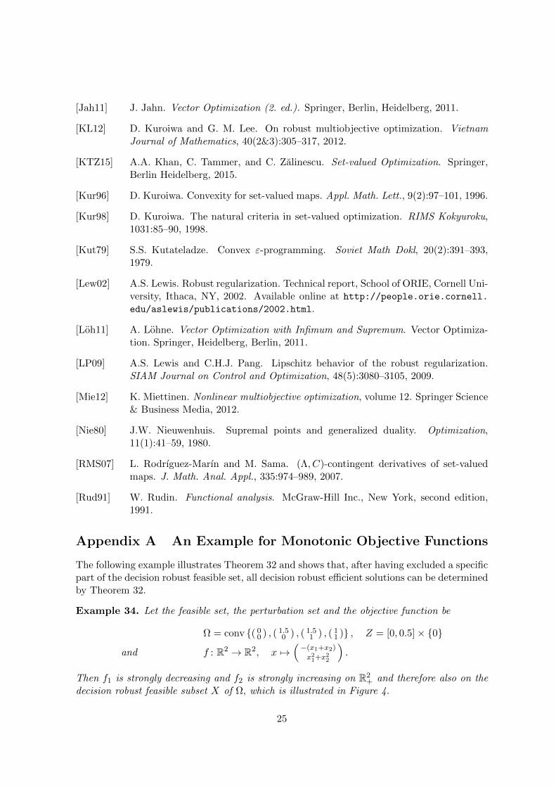
Example 34. Let the feasible set, the perturbation set and the objective function be

Ω = conv ( 00 ) , ( 1.5

0 ) , ( 1.51 ) , ( 1

1 ) , Z = [0, 0.5]× 0

and f : R2 → R2, x 7→(−(x1+x2)

x21+x22

).

Then f1 is strongly decreasing and f2 is strongly increasing on R2+ and therefore also on the

decision robust feasible subset X of Ω, which is illustrated in Figure 4.

25

x1

x2

1 2

1

2

Ω

x1

x2

1 2

1

2

X

Figure 4: The feasible set Ω and the decision robust feasible set X in Example 34.

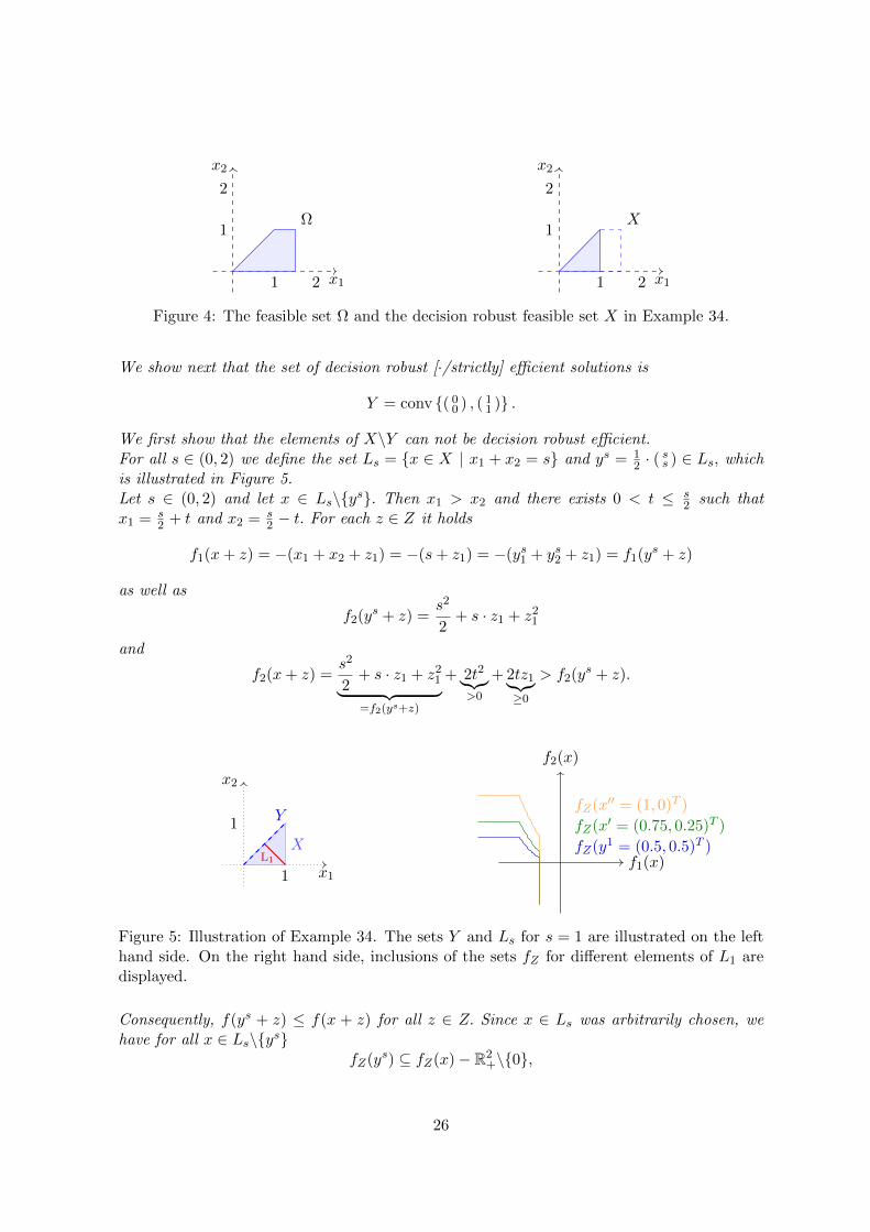
We show next that the set of decision robust [·/strictly] efficient solutions is

Y = conv ( 00 ) , ( 1

1 ) .

We first show that the elements of X\Y can not be decision robust efficient.For all s ∈ (0, 2) we define the set Ls = x ∈ X | x1 + x2 = s and ys = 1

2 · (ss ) ∈ Ls, which

is illustrated in Figure 5.Let s ∈ (0, 2) and let x ∈ Ls\ys. Then x1 > x2 and there exists 0 < t ≤ s

2 such thatx1 = s

2 + t and x2 = s2 − t. For each z ∈ Z it holds

f1(x+ z) = −(x1 + x2 + z1) = −(s+ z1) = −(ys1 + ys2 + z1) = f1(ys + z)

as well as

f2(ys + z) =s2

2+ s · z1 + z2

1

and

f2(x+ z) =s2

2+ s · z1 + z2

1︸ ︷︷ ︸=f2(ys+z)

+ 2t2︸︷︷︸>0

+ 2tz1︸︷︷︸≥0

> f2(ys + z).

x1

x2

1

1

X

Y

L1 f1(x)

f2(x)

fZ(y1 = (0.5, 0.5)T )

fZ(x′ = (0.75, 0.25)T )

fZ(x′′ = (1, 0)T )

Figure 5: Illustration of Example 34. The sets Y and Ls for s = 1 are illustrated on the lefthand side. On the right hand side, inclusions of the sets fZ for different elements of L1 aredisplayed.

Consequently, f(ys + z) ≤ f(x + z) for all z ∈ Z. Since x ∈ Ls was arbitrarily chosen, wehave for all x ∈ Ls\ys

fZ(ys) ⊆ fZ(x)− R2+\0,

26

which is visualized in Figure 5. Therefore, the set of decision robust [·/strictly] efficientsolutions is a subset of Y. Furthermore, because of the transitivity of 5, every element in Ythat is not decision robust [·/strictly] efficient is dominated by another element of Y. Since Yand Z are totally ordered with respect to 5, f1 is strongly de- and f2 is strongly increasing,Theorem 32 can be applied, leading to the conclusion that all y ∈ Y are decision robust[·/strictly] efficient.

27