Embed Size (px)
Citation preview
HAL Id: hal-00784077https://hal.archives-ouvertes.fr/hal-00784077
Submitted on 3 Feb 2013
HAL is a multi-disciplinary open accessarchive for the deposit and dissemination of sci-entific research documents, whether they are pub-lished or not. The documents may come fromteaching and research institutions in France orabroad, or from public or private research centers.
L’archive ouverte pluridisciplinaire HAL, estdestinée au dépôt et à la diffusion de documentsscientifiques de niveau recherche, publiés ou non,émanant des établissements d’enseignement et derecherche français ou étrangers, des laboratoirespublics ou privés.
Decoding by Embedding: Correct Decoding Radius andDMT Optimality
Laura Luzzi, Damien Stehlé, Cong Ling
To cite this version:Laura Luzzi, Damien Stehlé, Cong Ling. Decoding by Embedding: Correct Decoding Radius andDMT Optimality. IEEE Transactions on Information Theory, Institute of Electrical and ElectronicsEngineers, 2013, 59 (5), pp.2960-2973. �10.1109/TIT.2012.2236144�. �hal-00784077�
1
Decoding by Embedding: Correct Decoding Radiusand DMT Optimality
Laura Luzzi,Member, IEEE, Damien Stehle, and Cong Ling,Member, IEEE
Abstract—The closest vector problem (CVP) and shortest(nonzero) vector problem (SVP) are the core algorithmic prob-lems on Euclidean lattices. They are central to the applications oflattices in many problems of communications and cryptography.Kannan’s embedding technique is a powerful technique for solvingthe approximate CVP, yet its remarkable practical performanceis not well understood. In this paper, the embedding technique isanalyzed from abounded distance decoding (BDD) viewpoint. Wepresent two complementary analyses of the embedding technique:We establish a reduction from BDD to Hermite SVP (via uniqueSVP), which can be used along with any Hermite SVP solver(including, among others, the Lenstra, Lenstra and Lovasz (LLL)algorithm), and show that, in the special case of LLL, it performsat least as well as Babai’s nearest plane algorithm (LLL-aidedSIC). The former analysis helps to explain the folklore practicalobservation that unique SVP is easier than standard approximateSVP. It is proven that when the LLL algorithm is employed,the embedding technique can solve the CVP provided that thenoise norm is smaller than a decoding radiusλ1/(2γ), whereλ1 is the minimum distance of the lattice, andγ ≈ O(2n/4).This substantially improves the previously best known correctdecoding boundγ ≈ O(2n). Focusing on the applications of BDDto decoding of multiple-input multiple-output (MIMO) systems,we also prove that BDD of the regularized lattice is optimalin terms of the diversity-multiplexing gain tradeoff (DMT), andpropose practical variants of embedding decoding which requireno knowledge of the minimum distance of the lattice and/orfurther improve the error performance.
Index Terms—closest vector problem, lattice decoding, latticereduction, MIMO systems, shortest vector problem
I. I NTRODUCTION
Lattice decoding for the linear multiple-input multiple-output (MIMO) channel is a problem of high relevance inmulti-antenna, broadcast, multi-access, cooperative andothermulti-terminal communication systems [1, 2, 3]. Maximum-likelihood (ML) decoding for finite constellations carved from
This work was supported in part by a Royal Society-CNRS interna-tional joint project and by a Marie Curie Fellowship (FP7/2007-2013, grantagreement PIEF-GA-2010-274765). This work was presented inpart at theIEEE International Symposium on Information Theory (ISIT 2011), SaintPetersburg, Russia.
L. Luzzi was with the Department of Electrical and ElectronicEngi-neering, Imperial College London, London SW7 2AZ, United Kingdom.She is now with Laboratoire ETIS (ENSEA - Universite de Cergy-Pontoise- CNRS), 6 Avenue du Ponceau, 95014 Cergy-Pontoise, France (e-mail:[email protected]).
D. Stehle is with ENS de Lyon, Laboratoire LIP (U. Lyon, CNRS, ENSde Lyon, INRIA, UCBL), 46 Allee d’Italie, 69364 Lyon Cedex 07, France(e-mail: [email protected]).
C. Ling is with the Department of Electrical and Electronic Engineering,Imperial College London, London SW7 2AZ, United Kingdom (e-mail:[email protected]).
lattices can be realized efficiently by sphere decoding [4],whose complexity can however grow prohibitively with thedimensionn [5]. The decoding complexity is especially highin the case of coded or distributed systems, where the lat-tice dimension is usually larger [6, 7]. Thus, the practicalimplementation of decoders often has to resort to approximatesolutions, which mostly fall under two main strategies. Thefirst is to reduce the complexity of sphere decoding, notablyby pruning [8]. Another approach, which we investigate inthe present paper, is lattice reduction (LR)-aided decoding [9],which was used earlier by Babai in [10] and in essence applieszero-forcing (ZF), successive interference cancellation(SIC)or other suboptimal receivers to a reduced basis of the lattice.It was shown in [11] that regularized lattice-reduction aideddecoding can achieve the optimal diversity and multiplexingtradeoff (DMT) in MIMO fading channels. The proximityfactors that measure the gap between lattice-reduction-aideddecoding and (infinite) lattice decoding were derived in [12].Thanks to its average polynomial complexity [13, 14, 15], theLenstra, Lenstra and Lovasz (LLL) reduction [16] is widelyused in lattice decoding.
However, the analysis in [12] revealed that lattice-reduction-aided decoding exhibits a widening gap to (infinite) latticedecoding, so there is a strong demand for computationallyefficient suboptimal decoding algorithms that offer improvedperformance. Several such approaches are emerging, includingsampling [17] and embedding [18]. It was shown in [17] thatthe sampling technique can provide a constant improvementto the best known upper bound for the signal-to-noise ratio(SNR) gain with polynomial complexity.
Embedding decoding is especially appealing due toits excellent performance and polynomial complexity (ifpolynomial-complexity lattice reduction algorithms suchasLLL reduction are used). The core of the embedding techniqueis to embed ann-dimensional lattice and the received vectorinto an (n + 1)-dimensional lattice. By this means, ann-dimensional instance of the closest vector problem (CVP) isconverted into an(n+1)-dimensional instance of the shortest(nonzero) vector problem (SVP). The receiver extracts thetransmitted vector from a reduced basis of the extended lattice.
An “improved lattice reduction” technique that resemblesembedding was used for MIMO decoding in [19], but it is infact equivalent to LLL-aided SIC. It was recognized in [18]that the performance of the embedding technique could besignificantly improved by carefully choosing the embeddingparameter, leading to “augmented lattice reduction” (ALR).In particular, it was shown [18] that the LLL algorithm can
2
recover the transmitted vector when the noise norm is smallcompared to the minimum distanceλ1 of the lattice. Thiscondition corresponds to a variant of the CVP known asBounded Distance Decoding(BDD). More precisely,η-BDD(with η ≤ 1/2) is a special instance of the CVP where thenoise norm (or, equivalently, the distance from the target vectorto the lattice) is less thanR = η · λ1. The radiusR isreferred to as the (correct)decoding radiusof the algorithm.BDD instances appear both in coding and in cryptography.In coding theory, BDD is a suboptimal decoding strategythat enjoys lower complexity compared to ML decoding. Forspecific algebraic codes and for specific lattice codes, there arenumerous BDD algorithms that achieve optimalη = 1/2 inpolynomial-time [20, 21, 22]. On the other hand, for generallattices, polynomial complexity algorithms only solveη-BDDfor much smaller values ofη. The main general-purposeapproaches include: Babai’s ZF [10]; Babai’s SIC [10]; andthe randomized extensions by Klein [23], Lindner and Peik-ert [24], and Liuet al. [25].
In cryptography, the observed hardness of BDD has beenused as a constructive tool. The so-calledLearning WithErrors (LWE) problem [26] (see also the survey [27]) canbe interpreted as a variant of BDD where the lattice is chosenuniformly in a specific family of lattices and the noise vectorfollows a Gaussian distribution with small standard deviation.The apparent hardness of LWE in high dimensions has beenexploited to devise a number of cryptographic protocols,including encryption [26], identification [28] and signatureschemes [29].
The embedding technique is a powerful approach to BDDfor general lattices. Kannan seems to have been the first topropose this technique [30]. Since then, Micciancio has usedit to reduce the CVP to the SVP to prove certain hardnessresults [31], while Nguyen has employed it to break the GGHcryptosystem for parameters of practical interest [32]. Morerecently, in the context of cryptography, Lyubashevsky andMicciancio revealed a relationship between BDD and variantsof SVP [33]. Of particular relevance to this paper is therelationship between BDD and unique SVP (uSVP), a specialinstance of SVP for lattices whose second minimum is atleast γ times longer than the first minimum. It was shownin [33] that 1/(2γ)-BDD can be reduced toγ-uSVP. Thisrelation suggests the following strategy, already used in [18]:the embedding parameter should be chosen in such a way thatthe extended lattice exhibits an exponential gap between thefirst and second minimum, ensuring that LLL-reducing theextended lattice basis successfully solves the uSVP instance.
Contributions:Our contributions are twofold: We improvethe theoretical analysis of the embedding technique, and weconsider questions raised by the specific application of BDDand embedding to communications.
On the analysis front, we prove that embedding decodingusing the LLL algorithm can solve1/ (2γ)-BDD for γ ≈O(
√n2
n4 ). This is significantly better than the boundγ =
O(2n) proven in [18]. We propose two complementary proofsfor this result. In the first approach, we establish a reductionfrom the unique SVP to the Hermite SVP, which consists
in finding a non-zero vector of a given lattice, of smallnorm relative to the root determinant. This analysis can bespecialized to LLL by showing that the LLL algorithm cansolve γ-uSVP for γ ≈ O(2
n4 ). This is stronger than the
commonly used boundγ = O(2n2 ) in literature, which in fact
pertains to approximate SVP. The second approach consists inshowing Babai’s SIC achieves this correct decoding radius (byimproving the bound in [12]) and then proving that Kannan’sembedding with LLL performs at least as well as Babai’s SIC.For the latter component of this proof, we proceed by explic-itly following the steps performed by Kannan’s embedding.The two proofs are of independent interest. The first is notrestricted to LLL but is suited to any algorithm solving theHermite SVP, while the second provides a precise descriptionof how the embedding technique works.
The reduction from the unique SVP to the Hermite SVPhelps to explain the long-standing problem why unique SVP iseasier than standard approximate SVP. It has been known thatuSVP is potentially easier, and there has been experimentalevidence that this is indeed the case in practice [34]. However,no theoretic justification has been given before.
On the MIMO communications front, we prove that BDDof the regularized lattice is DMT-optimal over Rayleigh fadingchannels. This represents a nontrivial extension of the analysisin [11] for γ-approximation algorithms of CVP. Indeed, it willbe shown thatγ-approximate algorithms are a special case ofBDD, because any decoding technique which provides aγ-approximate CVP solution is also able to solve1/(2γ)-BDD.However, the converse is not necessarily true. In addition toembedding decoding, this result allows us to establish theDMT optimality of other BDD algorithms, such as latticereduction-aided decoding and sampling decoding.
For practical purposes, we consider the problem of choosingthe main parameter involved in Kannan’s embedding method,which we refer to as theembedding parameter. We givean alternative embedding parameter that only assumes theknowledge ofλ1 while achieving the same decoding radiusas [33]. We also consider the case whenλ1 is not known,and show that using multiple calls to this embedding decoderwith an estimate ofλ1 achieves essentially the same decodingradius as ifλ1 were known. On the experimental side, we pro-pose variants of the embedding technique without knowledgeof λ1 and/or with improved performance and compare themwith state-of-the-art MIMO decoding techniques by numericalsimulations in terms of error performance and complexity,showing that embedding is nearly optimal in many practicalscenarios.
The paper is organized as follows: Section II presents thetransmission model and a short survey of lattice problems. TheDMT analysis on BDD is given in Section III. In Section IV,we give the two analyses of the decoding radius of theembedding technique for solving BDD. In Section V, variantsof the embedding decoder are presented. Section VI evaluatesthe performance by computer simulation. Some concludingremarks are offered in Section VII.
Notation: Matrices and column vectors are denoted byupper and lowercase boldface letters, and the transpose, in-
3
verse, pseudoinverse of a matrixB by BT , B−1, and B†,respectively.In is the identity matrix of sizen. We let bi,bi,j and bi respectively denote thei-th column of matrixB,the entry in thei-th row and j-th column of B, and thei-th entry in vectorb. Vec(B) stands for the column-by-column vectorization of the matrixB. The inner product inthe Euclidean space between vectorsu and v is defined as〈u,v〉 = uTv, and the Euclidean norm‖u‖ =
√〈u,u〉.
Kronecker product of matrixA andB is written asA ⊗ B.If x is a real number, we let⌈x⌋ denote its rounding to aclosest integer. Theℜ and ℑ prefixes denote the real andimaginary parts. We use the standard asymptotic notationf (x) = O (g (x)) when lim supx→∞ |f(x)/g(x)| < ∞.
II. L ATTICE PROBLEMS IN MIMO D ECODING
A. System Model
Consider annT × nR flat-fading MIMO system modelconsisting ofnT transmitters andnR receivers
Y = HX+N, (1)
whereX ∈ CnT×T , Y, N ∈ C
nR×T of block lengthT denotethe channel input, output and noise, respectively, andH ∈C
nR×nT is the nR × nT full-rank channel gain matrix withnR ≥ nT , whose entries are normalized to unit variance. Theentries ofN are i.i.d. complex Gaussian with varianceσ2
each. The codewordsX satisfy the average power constraintE[‖X‖2F/T ] = 1. Hence, the signal-to-noise ratio (SNR) ateach receive antenna is1/σ2.
When a lattice space-time block code is employed, theQAM information vectorx is multiplied by the generatormatrix G of the encoding lattice. ThenT × T codewordmatrix X is defined by column-wise stacking of consecutivenT -tuples of the vectors = Gx ∈ C
nTT . By column-by-column vectorization of the matricesY and N in (1), i.e.,y = Vec(Y) and n = Vec(N), the received signal at thedestination can be expressed as
y =(IT ⊗H)Gx+ n. (2)
When T = 1 and G = InT, equation (2) reduces to the
model for uncoded MIMO communicationy = Hx + n.Furthermore, by separating real and imaginary parts, we obtainthe equivalent2nT × 2nR real-valued model
[ℜyℑy
]=
[ℜH −ℑHℑH ℜH
] [ℜxℑx
]+
[ℜnℑn
]. (3)
An equivalent2nTT×2nRT real model for coded MIMO canalso be obtained in a similar way.
The QAM constellationsC can be interpreted as the shiftedand scaled version of a finite subsetAnT of the integerlatticeZnT , i.e.,C = a(AnT +[1/2, ..., 1/2]T ), where the fac-tor a arises from energy normalization. For example, we haveAnT = {−
√M/2, ...,
√M/2− 1} for M-QAM signalling.
Therefore, with scaling and shifting, we consider thegenericn×m (with m ≥ n) real-valued MIMO system model
y = Bx+ n, (4)
where B ∈ Rm×n, given by the real-valued equivalent of
(IT ⊗H)G, can be interpreted as the basis matrix of the
decoding lattice. We haven = 2nTT andm = 2nRT . Thedata vectorx thus belongs to a finite subsetAn ⊂ Z
n whichsatisfies the average power constraint.
The maximum-likelihood (ML) decodercomputes
x = arg minx∈An
‖y −Bx‖2. (5)
The ML solution (5) can be found using the sphere decodingalgorithm, whose complexity, however, grows exponentiallywith n [5].A suboptimal alternative technique callednaive lattice de-coding (or simply lattice decoding) consists in relaxing theconstraint due to the signal constellation as follows:
x = arg minx∈Zn
‖y −Bx‖2.
A low-complexity approximation of lattice decoding issuc-cessive interference cancellation (SIC), also known as Babai’snearest plane algorithm [10]. It consists in performing theQRdecompositionB = QR, whereQ has orthonormal columnsandR is an upper triangular matrix with nonnegative diagonalelements [35]. Multiplying (4) on the left byQ†, we have
y′ = Q†y = Rx+ n′. (6)
An estimate ofx is then found by component-wise back-substitution and rounding:
xn =
⌊y′nrn,n
⌉,
xi =
⌊y′i −
∑nj=i+1 ri,j xj
ri,i
⌉, i = n− 1, . . . , 1.
B. Lattice Basics
We refer the reader to [36, 37] for thorough introductionsto Euclidean lattices. Ann-dimensional lattice in them-dimensional Euclidean spaceRm (n ≤ m) is the set ofinteger linear combinations ofn linearly independent vectorsb1, . . . ,bn ∈ R
m:
L={
n∑
i=1
xibi |xi ∈ Z, i = 1, . . . n
}.
The matrixB = [b1 · · ·bn] is referred to as a basis of the lat-tice L = L(B). In matrix form, we haveL = {Bx|x ∈ Z
n}.The dual latticeL∗ is defined as the set of those vectorsu, such that the inner product〈u,v〉 belongs toZ, forall v ∈ L. The dual basis ofB, which is a basis of thedual latticeL∗, is given byB∗ , (B†)TJ, whereJ is thecolumn-reversing matrix. IfR andR∗ respectively denote theR-factors of the QR-decomposition ofB and B∗, then wehaveri,i = 1/r∗n−i+1,n−i+1 for all i [38].
The determinantdetL ,√det(BTB) is independent of
the choice of the basis. Ashortest vectorof a latticeL is anon-zero vector inL with the smallest Euclidean norm. Thenorm of any shortest vector ofL, often referred to as theminimum distance, is denoted byλ1(L) or λ1(B) when abasisB is given. We also let it be denoted byλ1 if there is
4
no ambiguity concerning the lattice. The Hermite constant isdefined as
γn , supL
λ21(L)
det2/n L, (7)
where the supremum is taken over all lattices of dimensionn.There is currently no proof thatγn is an increasing functionof n, although this is very likely to be the case and all knownbounds onγn are increasing. For the sake of convenience, wedefine γn , maxni=1 γi. By Minkowski’s theorem [39], wehave the boundγn ≤ n and accordinglyγn ≤ n.
Let B (0,r) denote the closed ball of radiusr centeredat 0. The notion of minimum distance can be generalized, bydefining thei-th successive minimumλi(L) (or λi if there isno ambiguity on the lattice) as the smallest radiusr such thatB (0,r) contains at leasti linearly independent lattice points.If λ2 > γλ1 (with γ > 1), we say that the shortest vector inthe lattice isγ-unique.
For any pointy ∈Rm, the distance ofy to the latticeL isdenoted by dist(y,B) = minx∈Zn ‖y −Bx‖.
C. Lattice Problems
We now give precise definitions of the lattice problems thatare central to this work. In all these problems, the input latticeL is described by an arbitrary basisB.
• Closest Vector Problem (CVP):Given a latticeL and a vectory ∈ R
m, find a vectorBx ∈L such that‖y −Bx‖ is minimal.
• γ-Approximate CVP (γ-CVP), withγ ≥ 1:Given a latticeL and a vectory ∈ R
m, find a vectorBx ∈L such that‖y −Bx‖ ≤ γdist(y,B).
• η-Bounded Distance Decoding (η-BDD) with η ≤ 1/2:Given a latticeL and a vectory such that dist(y,B) < ηλ1,find the lattice vectorBx ∈ L (B) closest toy.
• Shortest Vector Problem (SVP):Given a latticeL, find a vectorv ∈ L of norm λ1.
• γ-Approximate SVP (γ-SVP), withγ ≥ 1:Given a latticeL, find a vectorv ∈ L such that0 < ‖v‖ ≤γλ1.
• Hermite SVP (C-HSVP), withC ≥ 1:Given a latticeL, find a vectorv ∈ L such that0 < ‖v‖ ≤C det1/n(L).
• γ-unique SVP (γ-uSVP), withγ ≥ 1:Given a latticeL such thatλ2(L) > γλ1(L), find a vectorv ∈ L of norm λ1.
D. LLL Reduction
A lattice of dimensionn ≥ 2 has infinitely many bases.In general, if B is a full column rank matrix, then everymatrix B = BU is also a basis ofL (B), when U is aunimodularmatrix, i.e.,det(U) = ±1 and all elements ofUare integers. The aim oflattice reductionis to find a “good”
basis for a given lattice. The celebrated LLL algorithm [16]was the first polynomial-time algorithm that computes a vectornot much longer than the shortest nonzero vector.
For the sake of simplicity of notation, in this paper weconsider the version of the LLL algorithm based on the QRdecomposition [40]B = QR. Let qi be the columns ofQ,andri,j be the elements ofR. Note thatr1,1 = ‖b1‖.
The basisB is calledLLL-reducedif
|rj,i| ≤1
2|rj,j | (8)
for 1 ≤ j < i ≤ n, and
δr2i−1,i−1 ≤ r2i,i + r2i−1,i (9)
for 1 < i ≤ n, where1/4 < δ ≤ 1 is a factor selected toachieve a good quality-complexity tradeoff.
Let α = 1/ (δ − 1/4). From Equations (8) and (9), an LLL-reduced basis satisfies the following property:
r2i,i ≥ α−1r2i−1,i−1, i = 2, . . . , n. (10)
The latter implies the following bounds (see [16]):
‖b1‖ ≤ α(n−1)/4det1/nL, (11)
‖b1‖ ≤ α(n−1)/2λ1. (12)
Equation (11) means that LLL solvesC-HSVP with C =α(n−1)/4, whereas Equation (12) implies that LLL solvesboth γ-SVP andγ-uSVP forγ = α(n−1)/2.
Remark 1:As this is the historical choice of [16] and asit simplifies (10), (11) and (12), one often setsδ = 3/4 andconsequentlyα = 2.
Remark 2:The complex LLL algorithm from [41] handlesa complex-valued lattice directly (without expanding it intoa real-valued lattice). It delivers a similar quality guaranteewith α = 1/ (δ − 1/2). The results of the present work canbe readily extended to complex LLL.
E. Lattice Reduction-Aided Decoding
In order to improve the performance of conventional de-coders (ZF or SIC), lattice reduction can be used to preprocessthe channel matrixB. Since the reduced channel matrix ismuch more likely to be well-conditioned, the effect of noiseamplification upon inverting the system will be moderated.The channel model (4) can be rewritten as
y = BU−1x+ n = Bx′ + n, x′ = U−1x, (13)
where B = BU and U is an unimodular matrix. The ZFor SIC estimatex′ for the equivalent channel (13) is thentransformed back intox = Ux′. As the resulting estimatex isnot necessarily inAn, remapping ofx onto the finite latticeAn
is required.The correct decoding radius of SIC is given by [12]
RSIC =1
2min
1≤i≤n|ri,i| , (14)
which means that correct decoding is guaranteed if‖n‖ ≤RSIC. Note that this bound is tight. If the basis is LLL-reduced,
5
the gap betweenmin |ri,i| and λ1 is bounded. Therefore,Babai’s nearest plane algorithm [10], or LLL-SIC, can beviewed as a basic BDD solver. By using (10) and the factthat‖b1‖ ≥ λ1, it can be proved that LLL-SIC solvesη-BDDfor η = 1
2α−(n−1)/2 (see [12]). Consequently, the decoding
radius of LLL-SIC is bounded as follows:
RLLL-SIC ≥ 1
2α(n−1)/2λ1. (15)
F. Improved bound on the decoding radius of LLL-SIC
Here, we derive an improved bound on the decoding radius,which is better than (15). To the best of our knowledge, thisis a new result of independent interest.
Lemma 1:The decoding radius of LLL-SIC satisfies
RLLL-SIC ≥ 1
2√γnα
(n−1)/4λ1 ≥ 1
2√nα(n−1)/4
λ1. (16)
Proof: Suppose the basisB is LLL-reduced. LetB =QR denote its QR-decomposition. By using (7) and (10), weobtain
λ1 ≤ √γk (detL[b1, · · · ,bk])
1/k
=√γk
(k∏
i=1
ri,i
)1/k
≤ √γkrk,k
(k−1∏
i=1
α(k−i)/2
)1/k
=√γkα
(k−1)/4rk,k. (17)
Now, by using (14) and the above, we have
RLLL-SIC =1
2min
1≤k≤n{rk,k}
≥ min1≤k≤n
1
2√γkα(k−1)/4
λ1
≥ 1
2√γnα
(n−1)/4λ1. (18)
This completes the proof.
III. DMT ANALYSIS OF BDD
In this section we will prove that any decoding technique forMIMO systems which provides a solution toη-BDD for someconstantη is optimal from the point of view of the diversity-multiplexing gain tradeoff or DMT [42], when a suitable leftpreprocessing is employed.
In the present discussion, we suppose for the sake ofsimplicity that m = n. Following the notation in [11], weconsider the equivalent normalized channel model where thenoise variance is equal to1:
y′ = B′x+ n′,
whereB′ =√ρB, n′
i =√ρni ∼ N (0, 1), ∀i = 1, . . . , n.
Here ρ = 1σ2 denotes the SNR. Moreover, we consider the
equivalent regularized system
y1 = Rx+ n1, (19)
where (B′
In
)= QR, y1 = Q†
(y
′
0n×1
).
From the point of view of receiver architecture, this amountsto performing left preprocessing before decoding, by usinga maximum mean square error generalized decision-feedbackequalizer (MMSE-GDFE) [43]. Note thatIn may be replacedwith any positive definite matrixT without hurting DMToptimality.
In [11], it was shown that when finite constellations areused, naive lattice decoding of the regularized system (19)without taking the constellation bounds into account is DMT-optimal. Moreover, it was proven that any decoding techniquethat always provides a solution toγ-CVP in the regularizedlattice for someγ is also DMT-optimal. Since LLL-SIC andLLL-ZF decoding applied to the regularized system turn outto solveγ-CVP, this means that MMSE-GDFE preprocessingfollowed by lattice-reduction aided decoding is also DMT-optimal.
It is easy to see that any decoding technique which providesa γ-CVP solutionx to (19) is also able to solve12γ -BDD. Infact, suppose thaty1 is such thatdist(y1,R) < 1
2γλ1(R).Then theγ-CVP solutionx satisfies
‖y1 −Rx‖<γ minx∈Zn
‖y1 −Rx‖ = γdist(y1,R) <λ1(R)
2,
so thatx is the optimal solution of (19).However, the converse is apparently not true, that is, BDD
does not necessarily provideγ-CVP solutions for ally1.Therefore, the analysis in [11] does not extend in a straightfor-ward manner to BDD of the regularized lattice. Nevertheless,we can show that DMT-optimality holds for all instancesof BDD, and not only forγ-CVP, by following the samereasoning of the original proof in [11].
Theorem 1:For any constantη > 0, any decoding tech-nique which always provides a solution for the regularizedη-BDD is DMT-optimal.
Proof: Let dML(r) be the optimal diversity gain corre-sponding to a multiplexing gainr ∈ {0, . . . ,min(nT , nR)}.Using the same notation as [11], we consider the constellationΛr ∩ R, where the latticeΛr = ρ−
rTn Z
n is scaled accordingto the SNR, andR is a fixed shaping region. LetB ⊂ R be aball of fixed radiusR, whereR is chosen in such a way thatd1 + d2 ∈ R, ∀d1,d2 ∈ B. Let
νr = mind∈B∩Λr
d 6=0
1
4‖B′d‖2 .
Then Lemma 1 of [11] holds, that is
lim supρ→∞
logP{νr ≤ 1}log ρ
≤ −dML(r).
Let ζ > 0 and chooseθ such that2ζTn > θ > 0. We haveΛr = ρ
ζTn Λr+ζ . As in the original proof, there existsρ1 such
that for anyρ ≥ ρ1, we haveR ⊆ 12ρ
ζTn B. As in Theorem 1
from [11], we want to show that the conditions
νr+ζ ≥ 1, ‖n′‖2 ≤ ρθ (20)
6
are sufficient for the regularizedη-BDD solver to decodecorrectly for sufficiently large SNR. First of all, we establisha lower bound for the minimum squared norm
d2R= min
x∈Λr\{0}
1
4‖Rx‖2 = min
x∈Λr\{0}
1
4
(‖B′x‖2 + ‖x‖2
).
as follows. Letϕ(x) = ‖B′x‖2 + ‖x‖2. Let x ∈ Λr \ {0} beany lattice point.
• If x /∈ 12ρ
ζTn B, thenϕ(x) ≥ ‖x‖2 > 1
4R2ρ
2ζTn .
• If x ∈ 12ρ
ζTn B ∩ Λr = 1
2ρζTn B ∩ ρ
ζTn Λr+ζ , then
xρ−ζTn ∈ 1
2B ∩ Λr+ζ and so14
∥∥∥B′xρ−ζTn
∥∥∥2
≥ 1 sinceby the hypothesis (20), we haveνr+ζ ≥ 1. Therefore weobtainϕ(x) ≥ ‖B′x‖2 ≥ 4ρ
2ζTn .
In conclusion, there existsk > 0 such thatd2R≥ kρ
2ζTn .
Now consider the transmitted codewordx ∈ Λr ∩ R.The regularizedη-BDD decoder is able to decode correctlyprovided that‖y1 −Rx‖ < ηdR. We have
‖y1 −Rx‖2 = ‖y′ −B′x‖2+‖x‖2 = ‖n′‖2+‖x‖2 ≤ ρθ+c,
where c = maxr∈R ‖r‖2 is a constant. Therefore underthe conditions (20), the regularizedη-BDD decoder is ableto decode correctly provided thatρθ + c < ηkρ
2ζTn . But
θ < 2ζTn , so there existsρ such that for anyρ ≥ ρ, we have
ρθ + c < ηkρ2ζTn . Then as in Theorem 1 from [11] we can
conclude that
P{xη−BDD 6= x} ≤ P{νr+ζ < 1}+ P{‖n′‖2 > ρθ}.
The second term is negligible forρ → ∞. So we can say,similarly to the original proof, that
lim supρ→∞
logP{xη−BDD 6= x}log ρ
≤ −dML(r + ζ)
and then use the right continuity ofdML(r).
IV. D ECODING RADIUS OF EMBEDDING
In this section we will review Kannan’s embedding tech-nique [30], show that it provides a BDD-solver, and analyzeits decoding radius.
The principle of this technique is to embed the basismatrix B and the received vectory into a higher dimensionallattice. More precisely, we consider the following(m+ 1)×(n+ 1) basis matrix:
B =
[B −y
01×n t
](21)
wheret > 0 is a parameter to be determined, which we referto as the embedding parameter. The strategy is to reduce CVPto SVP in the following way. For a suitable choice oft andfor sufficiently small noise norm, the vectors±v with v =[(Bx− y)T t]T are the shortest vectors in the latticeL(B).Thus an SVP algorithm will findv, and the messagex can berecovered from the coordinates of this vector in the basisB:
if v = B
(x′
1
)=
(Bx′ − y
t
), then x = x′. (22)
The LLL algorithm was used in [18] to find the shortestvector in the latticeL(B), and the correct decoding radiuswas shown to be lower bounded by
1
2√2αn− 1
2
λ1 (B) . (23)
when the parametert is set to 12√2αn/2
min1≤i≤n |ri,i|.In the following sections, we will derive improved bounds
on the decoding radius.
A. Reducing BDD to uSVP
In [33], it is proven that by choosingt = dist(y,B),the embedding technique allows one to reduce1/ (2γ)-BDDto γ-uSVP. We show that one can achieve the same correctdecoding radius by settingt = 1
2γλ1(B), thus bypassing theassumption from [33] thatdist(y,B) is known. In Section Vwe will show how to use an estimate ofλ1(B) to achievealmost the same decoding radius.
Theorem 2 (Decoding Radius of Embedding):Applying γ-uSVP (γ ≥ 1) to the extended lattice (21) with parametert(0 < t < λ1(B)/γ) guarantees a correct decoding radius
RuSVP-Emb≥√
t
γλ1(B)− t2. (24)
Settingt = 12γλ1(B) maximizes this lower bound. This gives:
RuSVP-Emb≥1
2γλ1(B). (25)
Remark 3: If the SVP itself is solved, then the correctdecoding radius satisfiesRuSVP-Emb≥ 1
2λ1(B). This result im-plies that embedding is more powerful than lattice reduction-aided SIC-decoding, since the latter still exhibits a wideninggap to 1
2λ1(B), which is at least polynomial inn for Korkin-Zolotarev reduction and for dual Korkin-Zolotarev reduction(which require to solve SVP instances) [12].
Theorem 2 is a direct consequence of the following lemma.Lemma 2:Let B be the matrix defined in (21), and let0 <
t < λ1(B)/γ, with γ ≥ 1. Suppose that
‖y −Bx‖ <
√t
γλ1(B)− t2.
Thenv =
(Bx− y
t
)is a γ-unique shortest vector ofL(B).
Proof: Let w be an arbitrary nonzero vector inL (B).Any vector inL(B) that is not a multiple ofv is of the form
w′ =
(w
0
)+ qv,
with q ∈ Z andw ∈ L(B) \ 0. We will show that‖w′‖ >γ‖v‖. The norm ofw′ can be written as
‖w′‖ =
√‖w − qn‖2 + (qt)
2,
wheren = y − Bx. If ‖qn‖ ≤ λ1(B), using the triangularinequality, we have‖w−qn‖ ≥ ‖w‖−q‖n‖ ≥ λ1(B)−q‖n‖.Thus we have the lower bound
‖w′‖ ≥√(λ1(B)− q ‖n‖)2 + (qt)
2
7
=
√λ1(B)2 − 2qλ1(B) ‖n‖+ q2 ‖n‖2 + q2t2
=
√√√√(‖n‖2 + t2)(
q − λ1(B) ‖n‖‖n‖2 + t2
)2
+λ1(B)2t2
‖n‖2 + t2
≥ λ1(B)t√‖n‖2 + t2
. (26)
If ‖qn‖ > λ1(B), we can also obtain the same bound because
‖w′‖ ≥ qt >λ1(B)t
‖n‖ ≥ λ1(B)t√‖n‖2 + t2
.
To prove that‖w′‖ > γ ‖v‖, it suffices to ensure that
λ1(B)t√‖n‖2 + t2
> γ
√‖n‖2 + t2.
This is implied by the assumption that
‖n‖2 = ‖Bx− y‖2 <t
γλ1(B)− t2.
As the LLL algorithm can solveγ-uSVP withγ = αn2 for
the basis (21) of dimensionn+1 (see Equation (12)), one canobtain that if using LLL, the correct decoding radius satisfies
RuSVP-Emb≥1
2αn2λ1(B) (27)
by choosingt = 1
2αn2λ1(B). This decoding radius improves
the bound (23) from [18]. However, it can still be improved.The reason is that the estimateγ = α
n2 is pessimistic forγ-
uSVP. In fact, the quantityαn2 is just the approximation factor
for the Approximate SVP achieved by LLL. Any algorithmsolving γ-SVP necessarily solvesγ-uSVP, while the converseis not true.
We now give two complementary approaches for improvingthe lower bound onRuSVP-Emb obtained by Kannan’s em-bedding based on LLL. In the first approach, described inSubsection IV-B, we provide a new reduction from HSVPto uSVP. This implies improved lower bounds on the correctdecoding radius for Kannan’s embedding based on any HSVPsolver.
For the second approach, we start by giving a new boundon the performance of LLL-SIC in Subsection II-F, whichis of independent interest. We then follow the execution ofLLL within Kannan’s embedding to show that it performs atleast as well as LLL-SIC (Subsection IV-C), which leads to animproved lower bound on the correct decoding radius achievedby Kannan’s embedding with LLL. This bound is slightlybetter (by a small constant factor) than the bound obtained byinstantiating the first approach with LLL. The first approachis more general, whereas the second approach gives furtherinsight on the relationship between Kannan’s embedding andLLL-SIC.
B. Reducing uSVP to HSVP
We describe a reduction from solvingγ-uSVP to solvingC-HSVP for γ ≈ √
nC. We will illustrate the usefulness of
this approach by considering several reduction algorithmssolvingC-HSVP with diverse time/quality trade-offs.
Theorem 3 (Reduction from uSVP to HSVP):Suppose thatthe sequence{Ck} is such that(Ck)
k/(k−1) increases withk.Then for any γ ≥ √
γn−1(Cn)n/(n−1), γ-uSVP reduces
to Cn-HSVP.Proof: Assume we have access to aCn-HSVP ora-
cle. Let L be ann-dimensional lattice such thatλ2(L) >√γn−1(Cn)
n/(n−1)λ1(L). Assume we are given a basisBof L. We use the HSVP oracle in the following way:
• Use the oracle on the dual latticeL∗ = L(B∗), to finda short vectorc∗1 ∈ L∗ in the dual lattice; Computethe largest integerk such thatc∗1 belongs tokL∗ anddividec∗1 by k; Extendc∗1 into a complete basisC∗ of L∗.This can be done in polynomial time by considering theunimodularn×n matrixV such that(c∗1)
tV is in HermiteNormal Form; the firstn− 1 rows of V −1 complete thebasis (see for example [44], Section 4).
• For i = 2, · · · , n: Project the vectorsc∗i , · · · , c∗nto the orthogonal complement of the space generatedby c∗1, . . . , c
∗i−1. Let c∗i , . . . , c
∗n be the projected vec-
tors. Note that the determinant of the projected latticeL([c∗i , . . . , c∗n]) is equal to
det(L∗)
det([c∗1, . . . , c∗i−1])
=det(L∗)∏i−1
j=1 r∗j,j
=
n∏
j=i
r∗j,j ,
whereC∗ = Q∗R∗ is the QR decomposition ofC∗.Apply the HSVP oracle again to find a short vector
v∗i =
n∑
k=i
xkc∗k
in the projected latticeL([c∗i , . . . , c∗n]); Lift it to a vectorv∗i in L([c∗i , . . . , c∗n]) given by
v∗i =
n∑
k=i
xkc∗k.
Then replacec∗i by v∗i and complete the dual basis. Since
lifting doesn’t affect the orthogonal projections nor ther∗i,i =< q∗
i ,v∗i >, the new basis satisfies
r∗i,i ≤ ‖v∗i ‖ ≤ Cn−i+1
n∏
j=i
r∗j,j
1n−i+1
and consequently
r∗i,i ≤ (Cn−i+1)n−i+1n−i
n∏
j=i+1
r∗j,j
1n−i
. (28)
This property still holds at subsequent steps of the algo-rithm since the operation of extracting a short vector andlifting decreasesr∗i,i, and so increases
∏nj=i+1 r
∗j,j .
We claim thatc1 in the primal basisC = (C∗)∗ is theshortest vectorv of L(B). We prove this fact by contradiction.Suppose thatc1 6= ±v, where±v are the unique shortest
8
vectors ofL. Note thatc1 cannot be±2v or other multiples,since in that caseC would not be a basis ofL. We may write
v =k∑
i=1
xici,
wherexi is an integer andk is the largesti such thatxi isnonzero.
Observe that ifC = QR is the QR decomposition ofC,
v =
k∑
i=1
xi
ri,iqi +
i−1∑
j=1
rj,iqj
=
k−1∑
i=1
xiri,i +
k∑
j=i+1
xjri,j
qi + xkrk,kqk.
Since theqi’s are orthogonal, we have:
λ1 ≥ ‖v‖ ≥ ‖rk,kqk‖ = rk,k.
Using the assumption thatc1 6= ±v, we have thatk > 1.This ensures that:
λ2 ≤ λ1(L [b1, . . . ,bk−1]).
Indeed, the second minimumλ2 must be no greater thanthe norm of the shortest nonzero vector in the sublatticespanned by{b1, . . . ,bk−1}, since these vectors are linearlyindependent withv. The fact thatk > 1 ensures that thereare non-zero vectors in that lattice. Using Minkowski’s firsttheorem, we obtain
λ2 ≤ √γk−1 det (L [b1, · · · ,bk−1])
1k−1
=√γk−1
(k−1∏
i=1
ri,i
) 1k−1
(29)
=√γk−1
(n∏
i=n−k+2
r∗i,i
)− 1k−1
,
where we used the relationri,i = 1/r∗n−i+1,n−i+1.In the meantime, the HSVP oracle (28) ensures that
r∗n−k+1,n−k+1 ≤ (Ck)k
k−1
(n∏
i=n−k+2
r∗i,i
) 1k−1
(30)
for any k > 1. Substituting into (29), we have
λ2 ≤ √γk−1(Ck)
kk−1 rk,k (31)
≤√γn−1(Cn)
nn−1λ1,
where we used the (mild) assumption that(Ck)k/(k−1) in-
creases withk. The last statement is a contradiction becausewe assumedλ2 >
√γn−1(Cn)
n/(n−1)λ1. This completes theproof.
We now instantiate Theorems 2 and 3 with two differentHSVP solvers.
The LLL algorithm solvesCn-HSVP with Cn = α(n−1)/4
(see Equation (11)). The sequence(Cn)n/(n−1) grows withn,
and thus, by Theorem 3, LLL solves anyn-dimensionalinstances ofγ-uSVP withγ =
√γn−1α
n/4. Note that in the
reduction from uSVP to HSVP (in the proof of Theorem 3), asingle LLL reduction suffices, even if the reduction calls theHSVP oracle many times on projections of the dual lattice.This is because LLL is almost self-dual and the projectedsublattices are also reduced. More precisely: We call a basiseffectivelyLLL-reduced if it satisfies condition (8) forj = i−1(and possibly not forj < i− 1) and if it satisfies the Lovaszcondition (9). A basis that is effectively LLL-reduced alsosatisfies Equations (10), (11) and (12). The LLL algorithm isself-dual in the sense that if a basis is effectively LLL-reduced,so is its dual basis (see [45]). Moreover, if[b1, . . . ,bn]is LLL-reduced, the projection of the basis[bi, . . . ,bn] onthe orthogonal complement of the vector space generated byb1, . . . ,bi−1 is also LLL-reduced.
Overall, if one relies on LLL as HSVP solver, we ob-tain that Kannan’s embedding achieves correct decoding ra-dius ≥ 1
2√
γnα(n+1)/4
λ1, when using embedding parameter
t = 1
2√
γnα(n+1)/4
λ1.
The BKZ algorithm [8] solvesC-HSVP with a smallerC,but at the cost of a higher run-time. It is parametrized bya block-sizeβ ∈ [2, n]. In [46], a variant of BKZ is given,which achievesCn,β = 2(γβ)
n−12(β−1)
+ 32 in time polynomial
in n and 2β . For a fixed value ofβ (and even for a block-size β that is growing slowly with respect ton), the se-quence(Cn,β)
n/(n−1) grows withn, and thus, by Theorem 3,the modified BKZ with block-sizeβ solves anyn-dimensionalinstances ofγ-uSVP withγ =
√γn(γβ)
n2(β−1)
+ 3n2(n−1) .
C. Embedding based on LLL is at least as good as LLL-SIC
The analysis in Subsection IV-B holds generally for anyHSVP solver. In this section we focus on the LLL algorithm,and prove a stronger bound, namely that embedding based onLLL has a decoding radius at least as large as LLL-SIC’s. Thekey observation is as follows: Ify falls within the decodingradius of Babai, the vector[(Bx − y)T t]T will be theshortest vector; it will be moved by LLL to the first column ofthe basis, and will stay there during the rest of the executionof LLL.
Lemma 3 (Embedding is at least as good as LLL-SIC):Consider a fixed realizationy = Bx+ n of the MIMOsystem (4). Suppose that‖n‖ < RLLL-SIC , so that the LLL-SIC decoder returns the correct transmitted vectorx. Thenthe embedding technique (based on LLL) with the choicet = RLLL-SIC also outputs the correct transmitted vector forthe same MIMO system. Consequently, the correct decodingradius of the embedding technique is greater or equal toRLLL-SIC .
Proof: Let Bred = BU be the LLL-reduced channelmatrix.
If Bred = QR is the QR decomposition ofBred, thenthe output of LLL-SIC is given byUx, where x is definedrecursively by
xi =
< qi,y >
ri,i−
n∑
j=i+1
ri,jri,i
xj
.
9
Suppose that the noise vectorn is shorter than the correctdecoding radius of LLL-SIC, that is
‖n‖ < RLLL-SIC =1
2min
1≤i≤n|ri,i| = t. (32)
Observe that the hypothesis of Lemma 2 is satisfied forγ =1, that is
√t(λ1(B)− t) ≥ RLLL-SIC = t > ‖n‖ , (33)
since λ1(B) ≥ 2RLLL-SIC . Consequently, Lemma 2 implies
that
(−n
t
)is a unique shortest vector in the extended lattice.
Consider an alternate version of LLL reduction in whicha full round of size reductions RED(k, i), i = k − 1, . . . , 1is performed before the Lovasz test, i.e., when consideringvector bk, the LLL variant ensures that condition (8) issatisfied for all|ri,k| / |ri,i| (with varying i) before checkingcondition (9). Since size reduction has no impact on the Lovasztest, this version leads to the same output as the usual LLLalgorithm [14]. After LLL-reducing the firstn columns, theaugmented channel matrix is of the form
B =
(Bred −y
0 t
)
By doing a first round of size reduction RED(n + 1, i),i = n, . . . , 1 on the last column, we find that the(n + 1)-th
column bn+1 =
(−n
t
), as size-reduction is exactly SIC. At
this stage, we have that augmented matrix is of the form(
bred1 . . . bred
n −n
0 . . . 0 t
).
We will prove by induction that for all the subsequent stepsindexed byk = n, . . . , 1, the Lovasz condition on the columnsk + 1 and k fails, and there is a swap, so that at stepk theaugmented matrix is of the form
B(k) =
(bred1 · · · bred
k −n ∗ · · · ∗0 . . . 0 t ∗ · · · ∗
).
The inductive step works as follows. LetB(k) = Q(k)R(k) bethe QR decomposition ofB(k). Then(r(k)k+1,k+1
)2+(r(k)k,k+1
)2≤∥∥∥r(k)k+1
∥∥∥2
≤∥∥∥b(k)
k+1
∥∥∥2
= ‖n‖2+t2
since the columns ofR(k) are projections of the correspondingcolumns ofB(k). All the swaps will take place since, becauseof condition (32),
‖n‖2 + t2 <1
2min
1≤l≤nr2l,l ≤
1
2r2k,k. (34)
After the last swap, we obtain
B(0) =
(−n ∗ . . . ∗t ∗ . . . ∗
).
Now, recall that if the first columnb1 of a basis matrix isa shortest lattice vector, then it remains at the first positionduring the whole execution of LLL. Indeed, it is neverswapped. To see it, recall that the swap between the first andthe second columns takes place only if‖b2‖2 < δ‖b1‖2. This
cannot occur asb2 6= 0 andb1 is a shortest non-zero latticevector.
Thanks to condition (33), the vector
(−n
t
)is a shortest
non-zero vector of the augmented lattice. So it is not swappedduring the subsequent steps of the execution of LLL, and thusit is the first column of the output basisBred.
To conclude, we have proven that with the choicet =RLLL-SIC , the correct decoding radius of embedding is greaterthanRLLL-SIC .
Remark 4:The proposed valuet = RLLL-SIC of the embed-ding parameter can be efficiently computed afterBred is foundand before reducing the(n+ 1)-th column ofB.
V. DEALING WITH λ1
The derived bounds on the correct decoding radius holdonly if the minimum distanceλ1 is known. However,λ1 canonly be obtained by solving SVP, which is generally a difficultproblem. Fortunately, there are alternative approaches that donot require the knowledge of the exact value ofλ1.
A. Rigorous approach
Suppose we do not knowλ1, but that we have a goodestimate of it:λ1 ∈ [A, κA] for some factorκ ≥ 1. Let
t = A2γ ∈
[λ1
2γκ ,λ1
2γ
]. The assumption of Theorem 2 is satisfied.
Observe that the right hand side of (24) is an non-decreasingfunction of t in this interval. Then the correct decoding radiusis
REmb =
√t
γλ1 − t2
≥ λ1
γ
√1
2κ− 1
4κ2
≥ λ1
γ
√1
2κ− 1
4κ
≥ λ1
2√κγ
. (35)
Equation (35) shows that for any approximation constantκ,we at most lose only a constant
√κ in the correct decoding
radius.We recall the following useful property of LLL-reducedB
which follows from (12):
α−(n−1)/2‖b1‖ ≤ λ1 ≤ ‖b1‖. (36)
Letting A = α−(n−1)/2‖b1‖, we obtain
A ≤ λ1 ≤ α(n−1)/2A. (37)
Substituting κ = α(n−1)/2 into (35) and choosingγ =√γnα
n+14 as in Subsection IV-B for(n + 1)-dimensional
lattices, we can obtain a decoding radius
R ≥ λ1
2√γnα
n/2,
by setting the embedding parametert to A2γ .
10
It is possible to obtain a better guarantee on the correctdecoding radius by partitioning the interval whereλ1 resides:
[A,α(n−1)/2A
]⊂
⌈n−12
log αlog κ ⌉⋃
i=0
[κiA, κi+1A
],
where κ > 1 is arbitrary. Each subinterval is of the form[Ai, Aiκ] with Ai = κiA. We apply the embedding techniquefor each subinterval, choosing
ti =Ai
2γ. (38)
Each call solvesγ-uSVP with γ =√γnα
n+14 as in Subsec-
tion IV-B for (n + 1)-dimensional lattices; at least one ofthese subintervals containsλ1
2γ , and therefore the correspond-ing call provides the closest lattice vector to the target aslong as the norm of the noise is less thanλ1
2γκ . Therefore,
using ⌈n−12
logαlog κ ⌉ calls to LLL, we can solveγ′-BDD with
γ′ =√κγ. That is, we only lose a factorκ, compared to the
case whenλ1 is known. Note thatκ can be chosen arbitrarilyclose to1, at the cost of increasing the number of calls toLLL.
B. Heuristic approach
We may also find a good estimate ofλ1 heuristically.There is a common belief that the worst-case bounds (11)
and (12) are not tight for LLL reduction on average. In lowdimensions, the LLL algorithm often finds the successiveminimum vectors in a lattice. In [47], the average behavior ofLLL reduction for some input distributions was numericallyassessed, and it was observed that one should replace the factorα
n−12 from (12) by a much smaller value for a random lattice
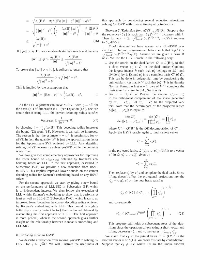
of sufficiently high dimension. The experiments correspondingto Fig. 1 allows one to observe a similar behavior for randombasis matrices with i.i.d. Gaussian entries: Forδ = 0.99,the factorα
n−12 ≈ (1.428)n−1 from (12) should be replaced
by ≈ 1.01n.Independently, we have the upper boundλ1 ≤√γnα
n−14 min1≤i≤n |ri,i| (from Lemma 1 and Equation (15)),
where the |ri,i|’s can be easily computed from the out-put basis. Forδ = 0.99, this approximately givesλ1 ≤√γn(1.195)
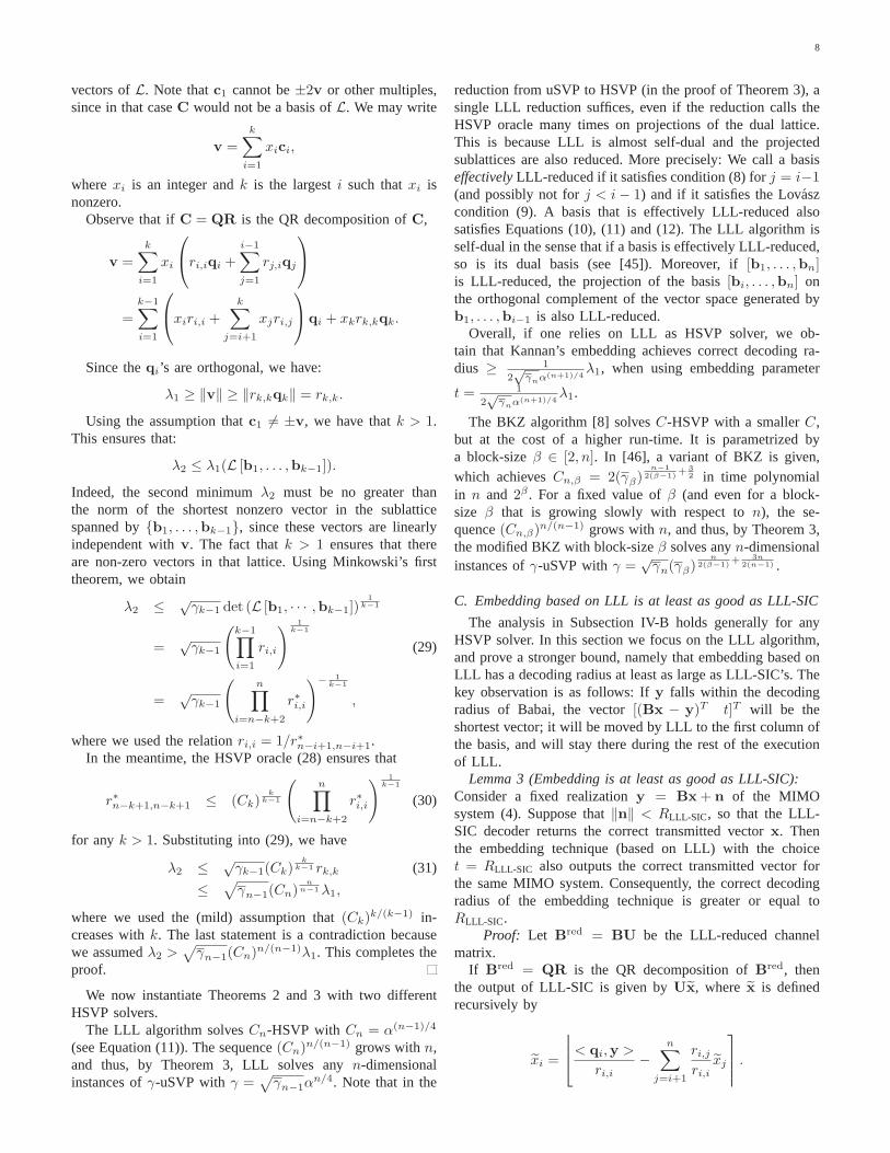
n−1 min1≤i≤n |ri,i|.Fig. 2 shows that after the call to LLL withδ = 0.99 and
for random input basis matrices with i.i.d. Gaussian entries,we haveλ1 ≈ 1.03n min1≤i≤n |ri,i|.
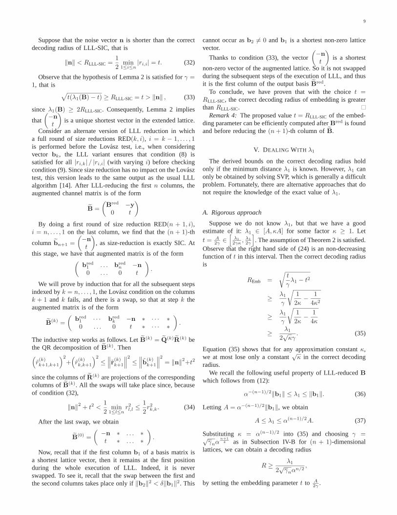
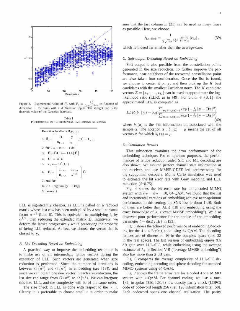
It is also folklore to estimateλ1 via the so-called Gaussianheuristic [48]
λ1
(detL)1/n ≈ Γ(1 + n/2)1/n√π
≈√
n
2πe.
This estimate ofλ1 is the radius of the ball whose volumematches the lattice determinant. The Gaussian heuristic holdsfor random lattices in a certain sense, and can be maderigorous for precise definitions of random lattices (derivedfrom the theory of Haar measures on classical groups) [47].However, the experiments in Fig. 3 tend to show that thisestimate does not apply for lattices sampled by i.i.d. Gaussian
0 10 20 30 40 500
0.001
0.002
0.003
0.004
0.005
0.006
0.007
0.008
0.009
0.01
Dimension n
log(
F1)/
n
Figure 1. Experimental value of1nlnF1 with F1 =
‖b1‖λ1
, as function ofdimensionn for the ouptut of LLL withδ = 0.99 and i.i.d. Gaussian inputs.
0 10 20 30 40 50−0.005
0
0.005
0.01
0.015
0.02
0.025
0.03
0.035
0.04
Dimension n
log(
F2)/
n
Figure 2. Experimental value of1nlogF2 with F2 = λ1
min1≤i≤n|ri,i|, as
function of dimensionn for the output of LLL with δ = 0.99 and i.i.d.Gaussian inputs.
matrices: the minimumλ1 seems to follow the Gaussianheuristic in the beginning, but to fall short of the theoreticvalue whenn is large.
VI. EXPERIMENTS
In this Section we address the practical implementationof embedding decoding in implementation and compare itsperformance with those of existing methods.
A. Incremental Reduction for Embedding
Setting t0 = A/(2γ) and κ = α1/2, we give an efficientimplementation of the strategy proposed in Section V-A wheren− 1 calls to LLL reduction of the extended matrix (21) areperformed for the sequence{ti} of values oft given in equa-tion (38). It is summarized by the pseudocode of the functionIncrEmb(B,y, t0) in Table I. Except the first one, each call to
11
0 10 20 30 40 500
0.5
1
1.5
2
2.5
3
Dimension n
F3
Figure 3. Experimental value ofF3 with F3 =λ21
(detL)2/nas function of
dimensionn, for bases with i.i.d. Gaussian inputs. The straight line isthetheoretic value of the Gaussian heuristic.
Table IPSEUDOCODE OF INCREMENTAL EMBEDDING DECODING
Function IncrEmb(B,y, t0)
1: B =
B −y
01×n t0
,U
′= In+1
2: for i = 1 to n− 1 do
3: B =BU←− LLL(B)
4: U′= U
′U
5: xi ←− U′(1, :)
6: B =
In×n 01×n
01×n α1/2
B
7: end for
8: x←−argmin ‖y −Bxi‖
9: return x
LLL is significantly cheaper, as LLL is called on a reducedmatrix whose last row has been multiplied by a small constantfactor α1/2 (Line 6). This is equivalent to multiplyingti byα1/2, then reducing the extended matrixB. Intuitively, wedeform the lattice progressively while preserving the propertyof being LLL-reduced. At last, we choose the vector that isclosest toy.
B. List Decoding Based on Embedding
A practical way to improve the embedding technique isto make use of all intermediate lattice vectors during theexecution of LLL. Such vectors are generated when sizereduction is performed. Since the number of iterations isbetweenO
(n2)
and O(n3)
in embedding (see [18]), andsince we can obtain one new vector in each size reduction, thelist size can range fromO
(n2)
to O(n4). We can integrate
this into LLL, and the complexity will be of the same order.The size check in LLL is done with respect to the|ri,i|.
Clearly it is preferable to choose smallt in order to make
sure that the last column in (21) can be used as many timesas possible. Here, we choose
tList-Emb =1
2√nα
n+14
min1≤i≤n
|ri,i| , (39)
which is indeed far smaller than the average-case.
C. Soft-output Decoding Based on Embedding
Soft output is also possible from the constellation pointsgenerated in the size reduction. To further improve the per-formance, near neighbors of the recovered constellation pointare also taken into consideration. Once the list is found,we choose to center it ony, and then pick up theK bestcandidates with the smallest Euclidean norm. TheK candidatevectorsZ = {z1, · · · , zK} can be used to approximate the log-likelihood ratio (LLR), as in [49]. For bitbi ∈ {0, 1}, theapproximated LLR is computed as
LLR (bi | y) = log
∑z∈Z:bi(z)=1 exp
(− 1
σ2 ‖y −Bz‖2)
∑z∈Z:bi(z)=0 exp
(− 1
σ2 ‖y −Bz‖2)
(40)where bi (z) is the i-th information bit associated with thesamplez. The notationz : bi (z) = µ means the set of allvectorsz for which bi (z) = µ.
D. Simulation Results
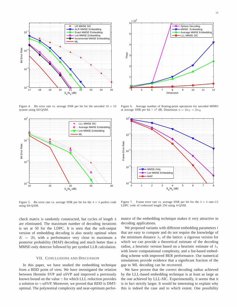
This subsection examines the error performance of theembedding technique. For comparison purposes, the perfor-mances of lattice reduction aided SIC and ML decoding arealso shown. We assume perfect channel state information atthe receiver, and use MMSE-GDFE left preprocessing forthe suboptimal decoders. Monte Carlo simulation was usedto estimate the bit error rate with Gray mapping and LLLreduction (δ=0.75).
Fig. 4 shows the bit error rate for an uncoded MIMOsystem withnT = nR = 10, 64-QAM. We found that the listand incremental versions of embedding achieve near-optimumperformance in this setting; the SNR loss is about1 dB. Bothof them are better than ALR [18] and embedding using theexact knowledge ofλ1 (“exact MMSE embedding”). We alsoobserved poor performance for the choice of the embeddingparametert = dist(y,B) in [33].
Fig. 5 shows the achieved performance of embedding decod-ing for the4× 4 Perfect code using64-QAM. The decodinglattices are of dimension 16 in the complex space (and 32in the real space). The list version of embedding enjoys3.5dB gain over LLL-SIC, while embedding using the averageestimate ofλ1 in Section V-B (“average MMSE embedding”)also has more than 2 dB gain.
Fig. 6 compares the average complexity of LLL-SIC de-coding, embedding decoding and sphere decoding for uncodedMIMO systems using 64-QAM.
Fig. 7 shows the frame error rate for a coded4× 4 MIMOsystem with 4-QAM. For channel coding, we use a rate-1/2, irregular (256, 128, 3) low-density parity-check (LDPC)code of codeword length 256 (i.e., 128 information bits) [50].Each codeword spans one channel realization. The parity
12
17 18 19 20 21 22 23 24 2510
−4
10−3
10−2
10−1
Eb/N
0 (dB)
Bit
Err
or R
ate
LR MMSE SICALR MMSE EmbeddingExact MMSE EmbeddingList MMSE EmbeddingIncremental MMSE EmbeddingML
Figure 4. Bit error rate vs. average SNR per bit for the uncoded 10 × 10system using 64-QAM.
10 15 20 25 3010
−3
10−2
10−1
100
Eb/N
0 (dB)
Bit
Err
or R
ate
LLL MMSE SICAverage MMSE EmbeddingList MMSE EmbeddingML
Figure 5. Bit error rate vs. average SNR per bit for the4× 4 perfect codeusing 64-QAM.
check matrix is randomly constructed, but cycles of length4are eliminated. The maximum number of decoding iterationsis set at 50 for the LDPC. It is seen that the soft-outputversion of embedding decoding is also nearly optimal whenK = 20, with a performance very close to maximum aposterior probability (MAP) decoding and much better than aMMSE-only detector followed by per symbol LLR calculation.
VII. C ONCLUSIONS ANDDISCUSSION
In this paper, we have studied the embedding techniquefrom a BDD point of view. We have investigated the relationbetween Hermite SVP and uSVP and improved a previouslyknown bound on the valueγ for which LLL reduction providesa solution toγ-uSVP. Moreover, we proved that BDD is DMT-optimal. The polynomial complexity and near-optimum perfor-
4 5 6 7 8 9 10 11 120
1
2
3
4
5
6x 10
5
Dimension
Flo
ps
Sphere DecodingMMSE EmbeddingAverage MMSE EmbeddingLLL MMSE SIC
Figure 6. Average number of floating-point operations for uncoded MIMOat average SNR per bit = 17 dB. Dimensionn = 2nT = 2nR
0 1 2 3 4 5 6 7 810
−4
10−3
10−2
10−1
100
Eb/N
0 (dB)
Fra
me
Err
or R
ate
MMSE OnlyList MMSE EmbeddingMAP
Figure 7. Frame error rate vs. average SNR per bit for the4 × 4 rate-1/2LDPC code of codeword length 256 using 4-QAM.
mance of the embedding technique makes it very attractive indecoding applications.
We proposed variants with different embedding parameterstthat are easy to compute and do not require the knowledge ofthe minimum distanceλ1 of the lattice: a rigorous version forwhich we can provide a theoretical estimate of the decodingradius, a heuristic version based on a heuristic estimate ofλ1
with lower computational complexity, and a list-based embed-ding scheme with improved BER performance. Our numericalsimulations provide evidence that a significant fraction ofthegap to ML decoding can be recovered.
We have proven that the correct decoding radius achievedby the LLL-based embedding technique is at least as large asthe one achieved by LLL-SIC. Experimentally, it seems that itis in fact strictly larger. It would be interesting to explain whythis is indeed the case and to which extent. One possibility
13
would be that the embedding technique benefits on averagefrom the noise vector following a normal distribution.
ACKNOWLEDGMENTS
The authors would like to thank Dr. Shuiyin Liu for runningsome of the computer simulations and helpful discussions.They also wish to thank the anonymous reviewers for theirdetailed comments and suggestions which helped to improvethe presentation of the paper.
REFERENCES
[1] W. H. Mow, “Maximum likelihood sequence estimation fromthe lattice viewpoint,”IEEE Trans. Inf. Theory, vol. 40, pp.1591–1600, Sep. 1994.
[2] M. O. Damen, H. E. Gamal, and G. Caire, “On maximumlikelihood detection and the search for the closest lattice point,”IEEE Trans. Inf. Theory, vol. 49, pp. 2389–2402, Oct. 2003.
[3] E. Agrell, T. Eriksson, A. Vardy, and K. Zeger, “Closest pointsearch in lattices,”IEEE Trans. Inf. Theory, vol. 48, pp. 2201–2214, Aug. 2002.
[4] E. Viterbo and J. Boutros, “A universal lattice code decoder forfading channels,”IEEE Trans. Inf. Theory, vol. 45, pp. 1639–1642, Jul. 1999.
[5] J. Jalden and B. Ottersten, “On the complexity of sphere de-coding in digital communications,”IEEE Trans. Signal Process.,vol. 53, pp. 1474–1484, Apr. 2005.
[6] F. Oggier, G. Rekaya, J.-C. Belfiore, and E. Viterbo, “Perfectspace time block codes,”IEEE Trans. Inf. Theory, vol. 52, pp.3885–3902, Sep. 2006.
[7] S. Yang and J. Belfiore, “Optimal space-time codes for theMIMO amplify-and-forward cooperative channel,”IEEE Trans.Inf. Theory, vol. 53, pp. 647–663, 2007.
[8] C. P. Schnorr and M. Euchner, “Lattice basis reduction: Im-proved practical algorithms and solving subset sum problems,”Math. Program., vol. 66, pp. 181–191, 1994.
[9] D. Wubben, D. Seethaler, J. Jalden, and G. Matz, “Lattice reduc-tion: A survey with applications in wireless communications,”IEEE Signal Process. Mag., pp. 70–91, May 2011.
[10] L. Babai, “On Lovasz’ lattice reduction and the nearest latticepoint problem,”Combinatorica, vol. 6, no. 1, pp. 1–13, 1986.
[11] J. Jalden and P. Elia, “DMT optimality of LR-aided lineardecoders for a general class of channels, lattice designs, andsystem models,”IEEE Trans. Inf. Theory, vol. 56, pp. 4765–4780, Oct. 2010.
[12] C. Ling, “On the proximity factors of lattice reduction-aideddecoding,”IEEE Trans. Signal Process., vol. 59, pp. 2795–2808,Jun. 2011.
[13] H. Daude and B. Vallee, “An upper bound on the averagenumber of iterations of the LLL algoirthm,”Theor. Comput.Sci., vol. 123, pp. 95–115, 1994.
[14] C. Ling and N. Howgrave-Graham, “Effective LLL reduc-tion for lattice decoding,” inProc. Int. Symp. Inform. Theory(ISIT’07), Nice, France, Jun. 2007.
[15] J. Jalden, D. Seethaler, and G. Matz, “Worst- and average-casecomplexity of LLL lattice reduction in MIMO wireless sys-tems,” in IEEE International Conference on Acoustics, Speechand Signal Processing (ICASSP), april 2008, pp. 2685 –2688.
[16] A. K. Lenstra, J. H. W. Lenstra, and L. Lovasz, “Factoringpolynomials with rational coefficients,”Math. Ann., vol. 261,pp. 515–534, 1982.
[17] S. Liu, C. Ling, and D. Stehle, “Decoding by sampling: Arandomized lattice algorithm for bounded-distance decoding,”IEEE Trans. Inf. Theory, vol. 57, pp. 5933–5945, Sep. 2011.
[18] L. Luzzi, G. Rekaya-Ben Othman, and J.-C. Belfiore, “Aug-mented lattice reduction for MIMO decoding,”IEEE Trans.Wireless Commun., vol. 9, pp. 2853–2859, Sep. 2010.
[19] N. Kim and H. Park, “Improved lattice reduction aided detec-tions for MIMO systems,” inProc. IEEE Veh. Tech. Conf., 2006.
[20] D. Chase, “A class of algorithms for decoding block codes withchannel measurement information,”IEEE Trans. Inf. Theory,vol. 18, pp. 170–182, Jan. 1972.
[21] G. D. Forney and A. Vardy, “Generalized minimum-distancedecoding for Euclidean-space codes and lattices,”IEEE Trans.Inf. Theory, vol. 42, pp. 1992–2026, Nov. 1996.
[22] D. Micciancio and A. Nicolosi, “Efficient bounded distancedecoders for Barnes-Wall lattices,” inInternational Symposiumon Information Theory – Proceedings of ISIT 2008. Toronto,Canada: IEEE, Jul. 2008.
[23] P. Klein, “Finding the closest lattice vector when it’s unusuallyclose,” Proc. ACM-SIAM Symposium on Discrete Algorithms,pp. 937–941, 2000.
[24] R. Lindner and C. Peikert, “Better key sizes (and attacks) forLWE-based encryption,” inCT-RSA, San Francisco, California,USA, Feb. 2011, pp. 319–339.
[25] Y.-K. Liu, V. Lyubashevsky, and D. Micciancio, “On boundeddistance decoding for general lattices,” inProc. APPROX andRANDOM 2006.
[26] O. Regev, “On lattices, learning with errors, random linearcodes, and cryptography,”J. ACM, vol. 56, no. 6, 2009.
[27] ——, “The learning with errors problem,” inIEEE Conferenceon Computational Complexity, 2010, pp. 191–204.
[28] E. Kiltz, K. Pietrzak, D. Cash, A. Jain, and D. Venturi, “Ef-ficient authentication from hard learning problems,” inProc.of EUROCRYPT, ser. Lecture Notes in Computer Science, vol.6632. Springer, 2011, pp. 7–26.
[29] V. Lyubashevsky, “Lattice signatures without trapdoors,” toappear in the proceedings of EUROCRYPT’12.
[30] R. Kannan, “Minkowski’s convex body theorem and integerprogramming,”Math. Oper. Res., vol. 12, pp. 415–440, Aug.1987.
[31] D. Micciancio and S. Goldwasser,Complexity of Lattice Prob-lems: A Cryptographic Perspective. Boston: Kluwer Academic,2002.
[32] P. Q. Nguyen, “Cryptanalysis of the Goldreich-Goldwasser-Halevi cryptosystem from crypto ’97,” inCRYPTO, 1999, pp.288–304.
[33] V. Lyubashevsky and D. Micciancio, “On bounded distancedecoding, unique shortest vectors, and the minimum distanceproblem,” in Crypto’09, Aug. 2009, pp. 577–594.
[34] N. Gama and P. Q. Nguyen, “Predicting lattice reduction,” inProc. Eurocrypt ’08. Springer, 2008.
[35] R. A. Horn and C. R. Johnson,Matrix Analysis. Cambridge,UK: Cambridge University Press, 1985.
[36] P. M. Gruber and C. G. Lekkerkerker,Geometry of Numbers.Amsterdam, Netherlands: Elsevier, 1987.
[37] J. W. S. Cassels,An Introduction to the Geometry of Numbers.Berlin, Germany: Springer-Verlag, 1971.
[38] J. C. Lagarias, W. H. Lenstra, and C. P. Schnorr, “Korkin-Zolotarev bases and successive minima of a lattice and itsreciprocal lattice,”Combinatorica, vol. 10, no. 4, pp. 333–348,1990.
[39] H. Minkowski, Geometrie der Zahlen, Leipzig, Germany, 1896.[40] D. Wuebben, R. Boehnke, V. Kuehn, and K. D. Kammeyer,
“Near-maximum-likelihood detection of MIMO systems usingMMSE-based lattice reduction,” inProc. IEEE Int. Conf. Com-mun. (ICC’04), Paris, France, Jun. 2004, pp. 798–802.
[41] Y. H. Gan, C. Ling, and W. H. Mow, “Complex lattice reductionalgorithm for low-complexity full-diversity MIMO detection,”IEEE Trans. Signal Process., vol. 57, pp. 2701–2710, Jul. 2009.
[42] L. Zheng and D. Tse, “Diversity and multiplexing: A funda-mental tradeoff in multiple antenna channels,”IEEE Trans. Inf.Theory, vol. 49 n.5, pp. 1073 – 1096, 2003.
[43] M. Damen, H. E. Gamal, and G. Caire, “MMSE-GDFE latticedecoding for solving under-determined linear systems withinteger unknowns,” inProc. IEEE Int. Symp. Inform. Theory,
14
2004.[44] S. S. Magliveras, T. V. Trung, and W. Wei, “Primitive sets in
a lattice,” Australasian Journal of Combinatorics, vol. 40, pp.173–186, 2008.
[45] N. Howgrave-Graham, “Finding small roots of univariate mod-ular equations revisited,” inProc. the 6th IMA Int. Conf. Crypt.Coding, 1997, pp. 131–142.
[46] G. Hanrot, X. Pujol, and D. Stehle, “Analyzing blockwise latticealgorithms using dynamical systems,” inAdvances in Cryptol-ogy - CRYPTO 2011 - 31st Annual Cryptology Conference,ser. Lecture Notes in Computer Science, vol. 6841. Springer-Verlag, 2011, pp. 447–464.
[47] P. Nguyen and D. Stehle, “LLL on the average,”Lecture Notesin Computer Science, vol. 4076, pp. 238–256, 2006, ANTS VII,Berlin, Germany, July 23-28, 2006.
[48] O. R. N. Gama, P. Q. Nguyen, “Lattice enumeration usingextreme pruning,” inProc. EUROCRYPT, 2010.
[49] B. M. Hochwald and S. ten Brink, “Achieving near-capacity ona multiple-antenna channel,”IEEE Trans. Commun., vol. 51,pp. 389–399, Mar. 2003.
[50] S. Lin and D. J. Costello,Error Control Coding, Second Edition.Upper Saddle River, NJ, USA: Prentice-Hall, Inc., 2004.
Laura Luzzi received the degree (Laurea) in Mathematics from the Universityof Pisa, Italy, in 2003 and the Ph.D. degree in Mathematics forTechnology andIndustrial Applications from Scuola Normale Superiore, Pisa, Italy, in 2007.From 2007 to 2012 she held postdoctoral positions in Telecom-ParisTechand Supelec, France, and a Marie Curie IEF Fellowship at Imperial CollegeLondon, United Kingdom. She is currently an Assistant Professor at ENSEAde Cergy, Cergy-Pontoise, France, and a researcher at Laboratoire ETIS(ENSEA - Universite de Cergy-Pontoise- CNRS).Her research interests include algebraic space-time codingand decoding forwireless communications and physical layer security.
Damien Stehle received his Ph.D. Degree in computer science from theUniversite Henri Poincare Nancy 1, France, in 2005. He has been a CNRSresearch fellow from 2006 to 2012, and is now Professor at ENSde Lyon.He is a member of the Aric INRIA team, within the Computer ScienceDepartment (LIP) of ENS de Lyon.His research interests include cryptography, algorithmic number theory, com-puter algebra and computer arithmetic, with emphasis on the algorithmicaspects of Euclidean lattices.
Cong Ling received the B.S. and M.S. degrees in electrical engineering fromthe Nanjing Institute of Communications Engineering, Nanjing, China, in 1995and 1997, respectively, and the Ph.D. degree in electrical engineering fromthe Nanyang Technological University, Singapore, in 2005.
He is currently a Senior Lecturer in the Electrical and Electronic Engineer-ing Department at Imperial College London. His research interests are coding,signal processing, and security, especially lattices. Before joining ImperialCollege, he had been on the faculties of Nanjing Institute ofCommunicationsEngineering and King’s College.
Dr. Ling is an Associate Editor of IEEE Transactions on Communications.He has also served as an Associate Editor of IEEE Transactions on VehicularTechnology.