Decomposing the ASASA Block CipherConstruction

Itai Dinur1, Orr Dunkelman2, Thorsten Kranz3, and Gregor Leander3

1 Departement d’Informatique, Ecole Normale Superieure, Paris, France2 Computer Science Department, University of Haifa, Israel

3 Horst Gortz Institute for IT-Security, Ruhr-Universitat Bochum, Germany

Abstract. We consider the problem of recovering the internal specifi-cation of a general SP-network consisting of three linear layers (A) in-terleaved with two Sbox layers (S) (denoted by ASASA for short), givenonly black-box access to the scheme. The decomposition of such generalASASA schemes was first considered at ASIACRYPT 2014 by Biryukovet al. which used the alleged difficulty of this problem to propose severalconcrete block cipher designs as candidates for white-box cryptography.In this paper, we present several attacks on general ASASA schemesthat significantly outperform the analysis of Biryukov et al. As a result,we are able to break all the proposed concrete ASASA constructionswith practical complexity. For example, we can decompose an ASASAstructure that was supposed to provide 64-bit security in roughly 228

steps, and break the scheme that supposedly provides 128-bit securityin about 241 time. Whenever possible, our findings are backed up withexperimental verifications.

Keywords: Block cipher, ASASA, white-box cryptography, integral crypt-analysis, differential cryptanalysis, Boomerang attack.

1 Introduction

In this paper we consider generic substitution permutation networks consistingof linear layers interleaved with Sbox layers. The linear layers considered arearbitrary linear bijections on the full state, whereas the Sbox layers partitionthe state into several fixed-size parts and apply a non-linear permutation toeach part in parallel. Special cases of this general set-up include a large varietyof well-known block ciphers, most prominently the AES.

Such constructions are far from being new. The first construction, due toPatarin and Goubin, is the ASAS construction, i.e., two rounds of a linear layer(A) followed by an Sbox layer (S) [14]. The scheme was later broken by Biham,exploiting the fact that the Sboxes were chosen to be non-bijective [1] (whichallowed for a simple differential attack).

Later, Biryukov and Shamir explored the general construction, denoted bySASAS (three Sbox layers and two linear layers) [4]. In the context of this system,the cryptanalytic task is to to recover the actual specification of the secret Sboxes

and linear layers, given only black-box access to the SP-network and its inverse.The attack is a generalization of the integral attack [11] (a.k.a. square attack)originally proposed by Knudsen as an attack on the cipher SQUARE [7]. It is thusa structural attack in nature, exploiting the fact that the SASAS construction iscomposed of only three permutation layers over a smaller alphabet interleavedwith linear layers, but ignoring the actual specification of these layers.

Besides the very general results of [4], several papers have focused on specialcases of the above scenario where more information about the internal structureis known. Most prominently, a case that has received considerable attention iswhere only the Sboxes are unknown but the specification of the linear layers iscompletely revealed to the attacker (see e.g. [5,15]).

Here we focus not on a special case of the most general setting but ratheron the natural complement of the SASAS structure, namely ASASA. That is,we consider an n-bit SP-network consisting of three linear (or affine) layers,interleaved with two Sbox layers, where each Sbox is a permutation over b bits.Our main motivation for analyzing this particular set-up was given by a recentproposal from ASIACRYPT 2014 [3] which constructed block ciphers with theadditional property of having memory-hard white-box implementations (see [3]for details). Such a block cipher is represented as a black-box (or a few black-boxes) describing how each input is mapped to an output. The goal of theadversary is to find a succinct representation of the given black-box mapping,which in our case implies recovering (or decomposing) the actual specificationsof the affine and Sbox layers.

Since the security of generic ASASA constructions was not previously an-alyzed, the authors of [3] supported their designs by claiming that they resiststandard attacks (such as differential and integral cryptanalysis, and boomerangattacks), essentially due to the external affine layers that hide the internal struc-ture of the Sboxes. The best generic attack on the ASASA construction proposedin [3] is a variant of the attack by Biryukov and Shamir on the SASAS structure,and is extremely inefficient, having time complexity of 2b(n−b). For example, [3]claims that an ASASA scheme with a block size of n = 16 and an Sbox size ofb = 8 provides security of 28(16−8) = 264.

It should be noted that [3] also uses a special case of the ASASA structurewith expanding Sboxes to construct strong white-box cryptography (again werefer to the paper for details) and that this part has been recently broken [8] byalgebraic cryptanalysis. However, those attacks do not seem to carry over to thegeneral ASASA case that we consider here.

1.1 Our Contribution

In this paper we describe several attacks that decompose the ASASA structuresignificantly faster than the 2b(n−b) complexity of [3]. Our most efficient attackshave time complexity of roughly n · 23n/2, and when applied to the specificinstances proposed in [3], they have practical complexities. For example, theASASA scheme with n = 16 and b = 8, which was claimed to provide securityof 264, can in fact be broken in 16 · 2(3·16)/2 = 228 time.

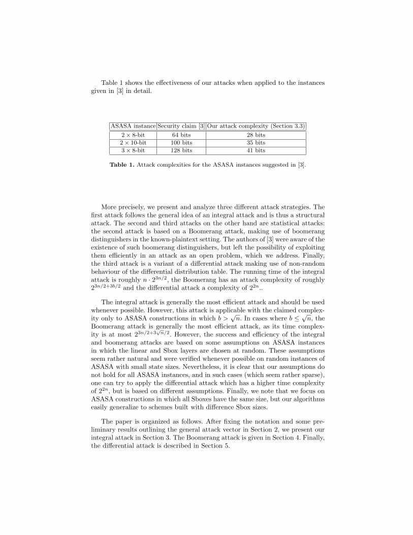
Table 1 shows the effectiveness of our attacks when applied to the instancesgiven in [3] in detail.

ASASA instance Security claim [3] Our attack complexity (Section 3.3)

2× 8-bit 64 bits 28 bits

2× 10-bit 100 bits 35 bits

3× 8-bit 128 bits 41 bits

Table 1. Attack complexities for the ASASA instances suggested in [3].

More precisely, we present and analyze three different attack strategies. Thefirst attack follows the general idea of an integral attack and is thus a structuralattack. The second and third attacks on the other hand are statistical attacks:the second attack is based on a Boomerang attack, making use of boomerangdistinguishers in the known-plaintext setting. The authors of [3] were aware of theexistence of such boomerang distinguishers, but left the possibility of exploitingthem efficiently in an attack as an open problem, which we address. Finally,the third attack is a variant of a differential attack making use of non-randombehaviour of the differential distribution table. The running time of the integralattack is roughly n · 23n/2, the Boomerang has an attack complexity of roughly23n/2+3b/2 and the differential attack a complexity of 22n..

The integral attack is generally the most efficient attack and should be usedwhenever possible. However, this attack is applicable with the claimed complex-ity only to ASASA constructions in which b >

√n. In cases where b ≤

√n, the

Boomerang attack is generally the most efficient attack, as its time complex-ity is at most 23n/2+3

√n/2. However, the success and efficiency of the integral

and boomerang attacks are based on some assumptions on ASASA instancesin which the linear and Sbox layers are chosen at random. These assumptionsseem rather natural and were verified whenever possible on random instances ofASASA with small state sizes. Nevertheless, it is clear that our assumptions donot hold for all ASASA instances, and in such cases (which seem rather sparse),one can try to apply the differential attack which has a higher time complexityof 22n, but is based on different assumptions. Finally, we note that we focus onASASA constructions in which all Sboxes have the same size, but our algorithmseasily generalize to schemes built with difference Sbox sizes.

The paper is organized as follows. After fixing the notation and some pre-liminary results outlining the general attack vector in Section 2, we present ourintegral attack in Section 3. The Boomerang attack is given in Section 4. Finally,the differential attack is described in Section 5.

2 Preliminaries

LetF : Fn2 → Fn2

be the ASASA construction with k Sboxes on b-bits each (n = kb). More pre-cisely, F is constructed as

F = L2 ◦ S1 ◦ L1 ◦ S0 ◦ L0

where Li are linear bijections on Fn2 and Si consist of parallel applications of kb-bit Sboxes. That is,

Si(x1, . . . , xk) =(S(1)i (x1), . . . , S

(k)i (xk)

)with xi ∈ Fb2

If we can recover the first linear layer, we are left with the SASA constructionthat can be decomposed very efficiently as shown in [4]. Thus, the aim of ourattacks is to recover L0 (or L2 by considering the inverse of F ). For this, firstnote that it is impossible – and unnecessary – to recover L0 exactly. This is dueto the fact that a given ASASA instance is not uniquely determined by F . Moreprecisely, replacing L0 by

L′0 =

T1T2...Tk

◦ L0

and S(i)0 by

S′(i)0 = S

(i)0 ◦ T

−1i ,

where Ti : Fb2 → Fb2 are linear bijections, results in the same ASASA instance F .This observation motivates the following definition.

Definition 1. Two linear bijections L and L′ on Fn2 are ASASA-equivalent ifthere exist linear bijections Ti on Fb2 such that

L′ =

T1T2...Tk

◦ LFor recovering L0 (up to equivalence) we are actually going to recover the

subspacesVi = L−10 (Ui)

whereUi = {(x1, x2, . . . , xk) | xj ∈ Fb2 and xj = 0 if j 6= i}.

As formalized in the proposition below, given the set of Vi’s basically determinesL0 up to (unavoidable) equivalences.

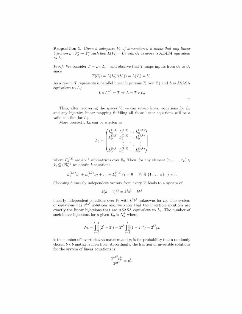
Proposition 1. Given k subspaces Vi of dimension b it holds that any linearbijection L : Fn2 → Fn2 such that L(Vi) = Ui with Ui as above is ASASA equivalentto L0.

Proof. We consider T = L ◦L−10 and observe that T maps inputs from Ui to Uisince

T (Ui) = L(L−10 (Ui)) = L(Vi) = Ui.

As a result, T represents k parallel linear bijections Ti over Fb2 and L is ASASAequivalent to L0:

L ◦ L−10 = T ⇒ L = T ◦ L0

ut

Thus, after recovering the spaces Vi we can set-up linear equations for L0

and any bijective linear mapping fulfilling all those linear equations will be avalid solution for L0.

More precisely, L0 can be written as

L0 =

L(1,1)0 L

(1,2)0 . . . L

(1,k)0

L(2,1)0 L

(2,2)0 . . . L

(2,k)0

......

. . ....

L(k,1)0 L

(k,2)0 . . . L

(k,k)0

where L

(i,j)0 are b× b submatrices over F2. Then, for any element (x1, . . . , xk) ∈

Vi ⊆ (Fb2)k we obtain b equations

L(j,1)0 x1 + L

(j,2)0 x2 + . . .+ L

(j,k)0 xk = 0 ∀j ∈ {1, . . . , k}, j 6= i.

Choosing b linearly independent vectors from every Vi leads to a system of

k(k − 1)b2 = k2b2 − kb2

linearly independent equations over F2 with k2b2 unknowns for L0. This systemof equations has 2kb

2

solutions and we know that the invertible solutions areexactly the linear bijections that are ASASA equivalent to L0. The number ofsuch linear bijections for a given L0 is Nk

b where

Nb =

b−1∏i=0

(2b − 2i) = 2b2

b∏i=1

(1− 2−i) = 2b2

pb

is the number of invertible b×b matrices and pb is the probability that a randomlychosen b× b matrix is invertible. Accordingly, the fraction of invertible solutionsfor the system of linear equations is

2kb2

pkb2kb2

= pkb .

Thus, if we know the set of Vi’s for an ASASA constructions with k b-bit Sboxes,we try out pkb solutions on average. Since pb > 2−1.792, it holds that

pkb > 2−1.792k

when considering constructions with up to k Sboxes. This step is completelyseparated from the attacks that find the set of Vi’s. Accordingly, the complexitiesdo not multiply and as we will see this step does not dominate the overall attackcomplexity.

Note that it is sufficient to know Vπ(i) for an unknown permutation π. Thesolution will then be a matrix which is ASASA equivalent to L0 with its rowspermuted according to π. This is also a valid solution as additionally permutingthe Sboxes in S1 and the columns in L1 results in the same ASASA instance.

3 Integral Attack

In this section we describe our integral attack on the ASASA construction. Westart by describing a basic integral attack that recovers the subspaces Vi fori ∈ {1, . . . , k} in time complexity of about n · 22n. Finally, we optimize theattack and reduce its time complexity to about n · 23n/2.

The analysis of the attack assumes that the parameters of the ASASA con-struction satisfy b > k, or equivalently b >

√n (and k <

√n). Moreover, it

assumes that the algebraic degree of the Sbox layers S0 and S1 and their in-verses is the maximal possible value of b − 1.4 We note that if the Sboxes areselected at random, then this will be the case with high probability. Addition-ally, the analysis is based on more subtle and heuristic (but natural) assumptionsthat we specify later in this section.

The starting point of the attack is the following integral property, which wasused to devise a related attack in the original ASASA paper [3]. We begin witha short definition, followed by the property and its proof.

Definition 2. Given a set R and x ∈ Fn2 , define R+ x , {x+ y | y ∈ R}

Proposition 2. Let x ∈ Fn2 and i ∈ {1, . . . , k}, then∑y∈Vi

F (x+ y) = 0.

Similar properties have been used before in integral and related attacks, mostnotably in the cryptanalysis of the SASAS structure [4]. It is possible to provethis property combinatorially (as done in [4]), but here we give an algebraicproof, as it is more relevant to the rest of this section. The proof is based on theuse of high-order derivatives (see [10,12] for details about high-order differentialcryptanalysis).

4 This condition can be somewhat relaxed, but we do not go into details for the sakeof simplicity.

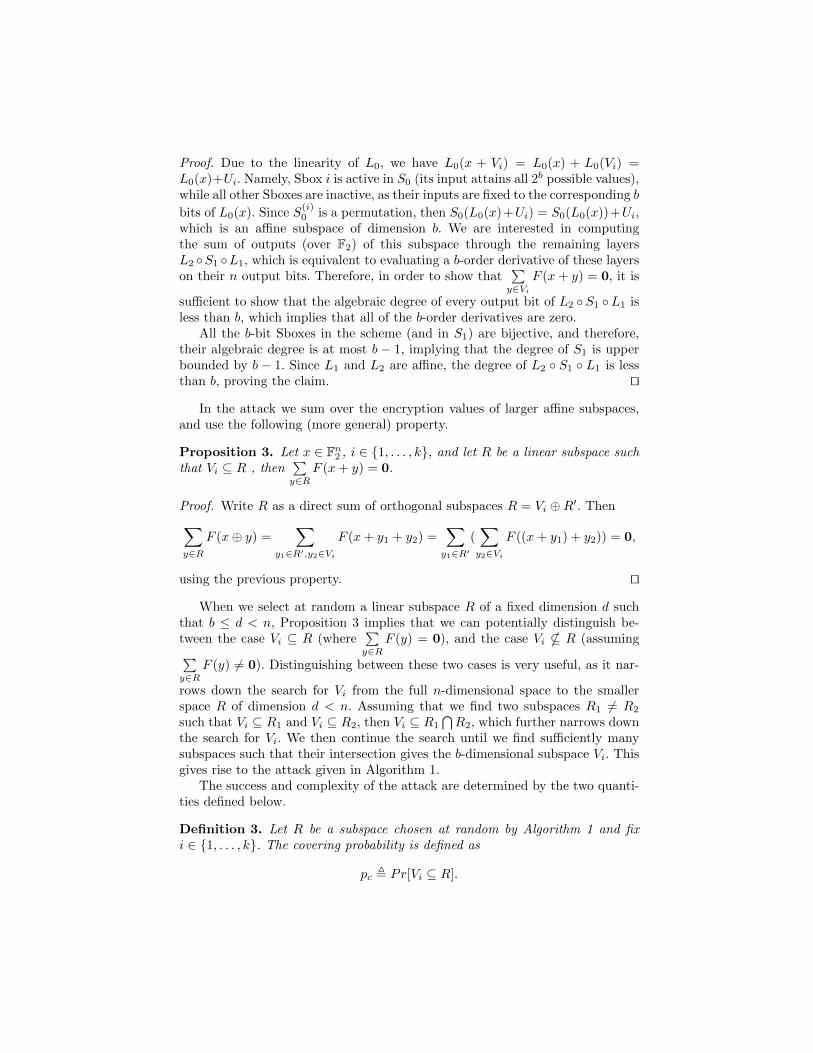
Proof. Due to the linearity of L0, we have L0(x + Vi) = L0(x) + L0(Vi) =L0(x)+Ui. Namely, Sbox i is active in S0 (its input attains all 2b possible values),while all other Sboxes are inactive, as their inputs are fixed to the corresponding b

bits of L0(x). Since S(i)0 is a permutation, then S0(L0(x)+Ui) = S0(L0(x))+Ui,

which is an affine subspace of dimension b. We are interested in computingthe sum of outputs (over F2) of this subspace through the remaining layersL2 ◦S1 ◦L1, which is equivalent to evaluating a b-order derivative of these layerson their n output bits. Therefore, in order to show that

∑y∈Vi

F (x+ y) = 0, it is

sufficient to show that the algebraic degree of every output bit of L2 ◦ S1 ◦L1 isless than b, which implies that all of the b-order derivatives are zero.

All the b-bit Sboxes in the scheme (and in S1) are bijective, and therefore,their algebraic degree is at most b − 1, implying that the degree of S1 is upperbounded by b − 1. Since L1 and L2 are affine, the degree of L2 ◦ S1 ◦ L1 is lessthan b, proving the claim. ut

In the attack we sum over the encryption values of larger affine subspaces,and use the following (more general) property.

Proposition 3. Let x ∈ Fn2 , i ∈ {1, . . . , k}, and let R be a linear subspace suchthat Vi ⊆ R , then

∑y∈R

F (x+ y) = 0.

Proof. Write R as a direct sum of orthogonal subspaces R = Vi ⊕R′. Then∑y∈R

F (x⊕ y) =∑

y1∈R′,y2∈Vi

F (x+ y1 + y2) =∑y1∈R′

(∑y2∈Vi

F ((x+ y1) + y2)) = 0,

using the previous property. ut

When we select at random a linear subspace R of a fixed dimension d suchthat b ≤ d < n, Proposition 3 implies that we can potentially distinguish be-tween the case Vi ⊆ R (where

∑y∈R

F (y) = 0), and the case Vi * R (assuming∑y∈R

F (y) 6= 0). Distinguishing between these two cases is very useful, as it nar-

rows down the search for Vi from the full n-dimensional space to the smallerspace R of dimension d < n. Assuming that we find two subspaces R1 6= R2

such that Vi ⊆ R1 and Vi ⊆ R2, then Vi ⊆ R1

⋂R2, which further narrows down

the search for Vi. We then continue the search until we find sufficiently manysubspaces such that their intersection gives the b-dimensional subspace Vi. Thisgives rise to the attack given in Algorithm 1.

The success and complexity of the attack are determined by the two quanti-ties defined below.

Definition 3. Let R be a subspace chosen at random by Algorithm 1 and fixi ∈ {1, . . . , k}. The covering probability is defined as

pc , Pr[Vi ⊆ R].

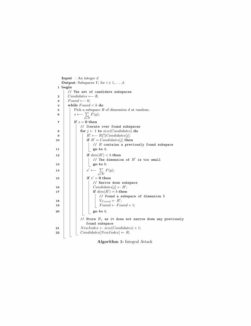
Input : An integer dOutput: Subspaces Vi for i ∈ 1, . . . , k

1 begin// The set of candidate subspaces

2 Candidates←− ∅;3 Found←− 0;4 while Found < k do5 Pick a subspace R of dimension d at random;6 s←−

∑y∈R

F (y);

7 if s = 0 then// Iterate over found subspaces

8 for j ← 1 to size(Candidates) do9 R′ ←− R

⋂Candidates[j];

10 if R′ = Candidates[j] then// R contains a previously found subspace

11 go to 4;

12 if dim(R′) < b then// The dimension of R′ is too small

13 go to 8;

14 s′ ←−∑

y∈R′F (y);

15 if s′ = 0 then// Narrow down subspace

16 Candidates[j]← R′;17 if dim(R′) = b then

// Found a subspace of dimension b18 VFound ← R′;19 Found← Found + 1;

20 go to 4;

// Store R, as it does not narrow down any previously

found subspace

21 NewIndex← size(Candidates) + 1;22 Candidates[NewIndex]← R;

Algorithm 1: Integral Attack

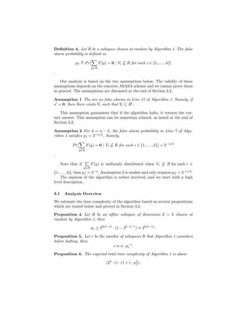
Definition 4. Let R be a subspace chosen at random by Algorithm 1. The falsealarm probability is defined as

pf , Pr[∑y∈R

F (y) = 0 | Vi * R for each i ∈ {1, . . . , k}]

.

Our analysis is based on the two assumptions below. The validity of theseassumptions depends on the concrete ASASA scheme and we cannot prove themin general. The assumptions are discussed at the end of Section 3.2.

Assumption 1 The are no false alarms in Line 15 of Algorithm 1. Namely, ifs′ = 0, then there exists Vi such that Vi ⊆ R′.

This assumption guarantees that if the algorithm halts, it returns the cor-rect answer. This assumption can be somewhat relaxed, as noted at the end ofSection 3.2.

Assumption 2 For d = n − k, the false alarm probability in Line 7 of Algo-rithm 1 satisfies pf < 2−n/2. Namely,

Pr[∑y∈R

F (y) = 0 | Vi * R for each i ∈ {1, . . . , k}] < 2−n/2

.

Note that if∑y∈R

F (y) is uniformly distributed when Vi * R for each i ∈

{1, . . . , k}, then pf = 2−n. Assumption 2 is weaker and only requires pf < 2−n/2.The analysis of the algorithm is rather involved, and we start with a high

level description.

3.1 Analysis Overview

We estimate the time complexity of the algorithm based on several propositionswhich are stated below and proved in Section 3.2.

Proposition 4. Let R be an affine subspace of dimension d > b chosen atrandom by Algorithm 1, then

pc ≥ 2b(d−n) · (1− 2b−d−1) ≈ 2b(d−n).

Proposition 5. Let e be the number of subspaces R that Algorithm 1 considersbefore halting, then

e ≈ n · p−1c .

Proposition 6. The expected total time complexity of Algorithm 1 is about

(2d · e) · (1 + e · p2f ).

Plugging the value of pc obtained from Proposition 4 into the value of e,obtained from Proposition 5, we get

e ≈ n · p−1c ≈ n · 2b(n−d).

Plugging this value of e into the total time complexity of the attack obtainedfrom Proposition 6, we can conclude that it is preferable to select the largestdimension d which does not significantly affect pf . However, according to theupper-bound of Proposition 7, we cannot take d too large, as this will result inpf = 1, causing the algorithm to fail (or to be extremely inefficient). We notethat unlike the previous propositions, the upper bound on d is not directly usedin the complexity analysis of the attack, but rather restricts the possible choiceof parameters.

Proposition 7. Assume that the parameters of the ASASA construction satisfyb > k and d > n− k, then pf = 1.

Since we require pf < 1, we select the maximal possible value for which thismay occur, namely d = n− k. According to Proposition 4,

pc ≈ 2b(d−n) = 2−bk = 2−n.

Plugging the value pc = 2−n into the expression obtained in Proposition 5, weget

e ≈ n · p−1c ≈ n · 2n.

The total time complexity of the attack is estimated in Proposition 6 as(2d · e) · (1 + e · p2f ), where e ≈ n · 2n. According to Assumption 2, pf < 2−n/2,

implying that 1 + e · p2f ≈ 1 and the time complexity of the algorithm is about

2d · e ≈ n · 22n,

since d = n− k ≈ n when k <√n.

3.2 Detailed Analysis

In this section we prove the propositions stated above and consider the assump-tions 1 and 2.

Proof of Proposition 4 Let (a1, . . . , ab) be an arbitrary basis of Vi. We haveVi ⊆ R if and only if aj ∈ R for j ∈ {1, . . . , b}. Since R is a random d-dimensionalsubspace, then Pr[a1 ∈ R] = 2d−n. Next, since a1 and a2 are linearly indepen-dent Pr[a2 ∈ R | a1 ∈ R] = 2d−n − 2−n, and Pr[{a1, a2} ⊆ R] = Pr[a1 ∈R] · Pr[a2 ∈ R | a1 ∈ R] = 2d−n · (2d−n − 2−n).

In general, for j > 1

Pr[{a1, . . . , aj} ⊆ R | {a1, . . . , aj−1} ⊆ R] = 2d−n − 2j−2−n

and therefore

pc = Pr[{a1, . . . , ab} ⊆ R] =

Pr[{a1, . . . , ab} ⊆ R | {a1, . . . , ab−1} ⊆ R] · Pr[{a1, . . . , ab−1} ⊆ R] =

Pr[a1 ∈ R] ·b∏j=2

Pr[{a1, . . . , aj} ⊆ R | {a1, . . . , aj−1} ⊆ R] >

b∏j=1

(2d−n − 2j−2−n) =

(2d−n)b ·b∏j=1

(1− 2j−2−d) ≥

2b(d−n) · (1− 2b−d−1),

where the last inequality can be easily proved by induction. ut

Proof of Proposition 5 We estimate e as follows. Fix i ∈ {1, . . . , k} andlet R1, . . . , Rt be t random d-dimensional subspaces under the restriction thatVi ⊆ Rj for each j ∈ {1, . . . , t}. Since each subspace Rj is of dimension n− k, it

is easy to see that for t = n/k = b, with good probability,t⋂

j=1

Rj = Vi (as every

subspace in the sequence is expected to reduce the dimension of the intersectionby about k, until the intersection is equal to Vi). Therefore, after about b · p−1cchoices of random subsets, we expect that Vi will be recovered in Line 18. Notethat this assumes that there are no false alarms in Line 15, as such false alarms

will disrupt the sequencet⋂

j=1

Rj , stored in memory.5 In order to recover all Vi

for i ∈ {1, . . . , k}, we need to try about

e ≈ log(k) · b · p−1c < n · p−1c

random subsets of dimension d = n− k. ut

Proof of Proposition 6 The time complexity of summing over all the d-dimensional subspaces in Line 6 of the attack is e · 2d. Moreover, there areadditional operations on the set of candidates that we need to take into account.At the end of the attack, the size of the stored subspaces in Candidates dependson pf and is about e · pf , in addition to the k subspaces which are not falsealarms. Therefore, at the end of the attack size(Candidates) ≈ k + e · pf ≈e · pf . Every candidate subspace R is intersected with all previous subspacesin Candidates, and the sum over the intersection R′ is computed. In total, the

5 We also assume that we did not select R such that Vi ⊆ R and Vj ⊆ R for i 6= j.This is event is very unlikely and can be ignored.

amount of additional work for the candidates is dominated by Line 14 and isabout (e · pf )2 · 2d. The total time complexity of the attack is about

e · 2d + (e · pf )2 · 2d = (2d · e) · (1 + e · p2f ).

ut

Proof of Proposition 7 Assume that d > n−k, and we want to show that pf =1. Since R is a linear subspace, the expression

∑y∈R

F (y) evaluates a derivative

of F of order higher than n − k for each of the n output bits. Therefore, it issufficient to show that deg(F ) < n − k + 1, which implies that the outcome ofthe derivation is zero regardless of R. In other words, Pr[

∑y∈R

F (y) = 0] = 1, and

this holds in particular if Vi * R for each i ∈ {1, . . . , k}, implying pf = 1.The fact that deg(F ) < n − k + 1 is derived from a theorem due to Boura

and Canteaut in [6] (stated below in a slightly modified form).

Theorem 1 ([6]). Let H be a permutation of Fn2 and let G be a function fromFn2 to Fn2 . Then we have

deg(G ◦H) < n− bn− 1− deg(G)

deg(H−1)c

.

In our case, let H = L1◦S0◦L0 and G = L2◦S1, then deg(G) = deg(H−1) =b− 1 (as assumed at the beginning of the section). Therefore,

deg(F ) < n− bn− 1− b− 1

b− 1c = n− bbk − b

b− 1c =

n− b (b− 1)(k − 1) + (k − 1)

b− 1c =

n− (k − 1) + bk − 1

b− 1c = n− k + 1,

as k < b.ut

Assumptions on False Alarms Assumption 1 states that false alarms do notoccur in Line 15 of Algorithm 1. A false alarm in Line 15 occurs in case thereare false alarms for both R and the smaller subspace R′ ⊆ R. This event issignificantly less likely than pf , but may occur nevertheless. Therefore, we relaxthe assumption and slightly modify the algorithm to deal with such false alarms:in case s′ = 0 in Line 15, before updating the candidate list we add an additionalfiltering to test the condition Vi ⊆ R′. This is done by selecting at randoma vector x which is not in R′, and testing whether

∑y∈span({x}

⋃R′)

F (y) = 0.

The additional filtering will not result in deterioration in performance (again,assuming false alarms in Line 15 do not occur often).

Recall that in the attack we evaluate arbitrary d-order derivatives of F , andtherefore the value of pf in Assumption 2 depends on the density of monomials ofdegree (at least) d in its algebraic normal form. We select the maximal possiblevalue d = n− k for which it is theoretically possible that deg(F ) ≤ d, or pf < 1(and in particular, we assume that pf < 2−n/2). Indeed, as shown above, thebound due to [6] implies that deg(F ) < n − k + 1, but does not rule out thepossibility that deg(F ) = n − k. Moreover, the trivial bound on the algebraicdegree of F gives deg(S0) · deg(S1) = (b− 1) · (b− 1) ≥ (

√n)2 = n > n− k, and

does not contradict the possibility that deg(F ) = n− k.

Our experiments of toy ASASA variants confirm our assumption about pf .In fact, for ASASA schemes with 2 or 3 Sboxes,

∑y∈R

F (y) was almost uniformly

distributed when Vi * R for each i ∈ {1, . . . , k}, namely pf ≈ 2−n.

3.3 Optimized Integral Attack

The basic integral attack sums the outputs of e ≈ n ·2n subspaces, each contain-ing 2d = 2n−k ≈ 2n elements. Therefore, its total time complexity is about n·22n.The complexity of summing over the subspaces can be significantly reduced ifwe choose correlated subspaces instead of picking them at random. More specif-ically, as we show next, it is possible to sum over the outputs of 2n/2 carefullychosen subspaces in about 2n time. This reduces the complexity of the attack toabout n · 23n/2 under the assumption that pf < 2−3n/4, which is stronger thanthe assumption made in the basic attack.

One way to optimize the summation process is to divide the n-bit block intotwo equal halves (assuming n is even). First, for each value of the n/2 mostsignificant bits (MSBs), compute the sums over the outputs of all possible 2n/2

values of the n/2 least significant bits (LSBs). This gives an array of partial sumsof size 2n/2 which is computed in time 2n. Next, choose a subspace of dimensiond−n/2 from the n/2 MSBs, and sum over the outputs of the bigger subspace ofdimension d that includes the n/2 LSBs. Using the recomputed array, this canbe done in time 2d−n/2. Repeating the process for 2n/2 subspaces of dimension2d−n/2, the sums over the outputs of all of them can be computed in about 2d

time using the precomputed array. In total, we sum over the outputs of 2n/2

subspaces in about 2n time, as claimed.

In general, instead of dividing the bits of the block into two halves, we canwork with two orthogonal subspaces of dimension n/2. The pseudocode of thegeneral procedure is given in Algorithm 2.

We consider slightly modify definitions 3 and 4 which refer to subspaces se-lected according to the procedure of Algorithm 2. The analysis at the end of thissection shows that the covering probability of the algorithm pc remains roughly2−n, and thus the attack still requires evaluating e ≈ n ·2n subspaces. The sums

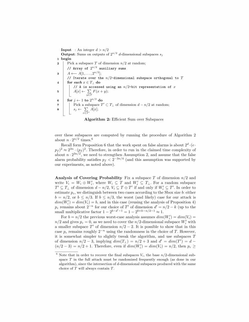
Input : An integer d > n/2Output: Sums on outputs of 2n/2 d-dimensional subspaces sj

1 begin2 Pick a subspace T of dimension n/2 at random;

// Array of 2n/2 auxiliary sums

3 A←− A[1, . . . , 2n/2];// Iterate over the n/2-dimensional subspace orthogonal to T

4 for each x ∈ T⊥ do// A is accessed using an n/2-bit representation of x

5 A[x]←∑y∈T

F (x + y);

6 for j ← 1 to 2n/2 do7 Pick a subspace T ′ ⊂ T⊥ of dimension d− n/2 at random;8 sj ←

∑x∈T ′

A[x];

Algorithm 2: Efficient Sum over Subspaces

over these subspaces are computed by running the procedure of Algorithm 2about n · 2n/2 times.6

Recall form Proposition 6 that the work spent on false alarms is about 2d ·(e ·pf )2 ≈ 23n · (pf )2. Therefore, in order to run in the claimed time complexity ofabout n · 23n/2, we need to strengthen Assumption 2, and assume that the falsealarm probability satisfies pf < 2−3n/4 (and this assumption was supported byour experiments, as noted above).

Analysis of Covering Probability Fix a subspace T of dimension n/2 andwrite Vi = Wi ⊕ W ′i , where Wi ⊆ T and W ′i ⊆ T⊥. For a random subspaceT ′ ⊆ T⊥ of dimension d− n/2, Vi ⊆ T ⊕ T ′ if and only if W ′i ⊆ T ′. In order toestimate pc, we distinguish between two cases according to the Sbox size b: eitherb = n/2, or b ≤ n/3. If b ≤ n/3, the worst (and likely) case for our attack isdim(W ′i ) = dim(Vi) = b, and in this case (reusing the analysis of Proposition 4)pc remains about 2−n for our choice of T ′ of dimension d′ = n/2− k (up to thesmall multiplicative factor 1− 2b−d

′−1 = 1− 2b+k−n/2−1 ≈ 1.

For b = n/2 the previous worst-case analysis assumes dim(W ′i ) = dim(Vi) =n/2 and gives pc = 0, as we need to cover the n/2-dimensional subspace W ′i witha smaller subspace T ′ of dimension n/2 − 2. It is possible to show that in thiscase pc remains roughly 2−n using the randomness in the choice of T . However,it is somewhat simpler to slightly tweak the algorithm, and use subspaces Tof dimension n/2 − 3, implying dim(T⊥) = n/2 + 3 and d′ = dim(T ′) = d −(n/2 − 3) = n/2 + 1. Therefore, even if dim(W ′i ) = dim(Vi) = n/2, then pc ≥

6 Note that in order to recover the final subspaces Vi, the base n/2-dimensional sub-space T in the full attack must be randomized frequently enough (as done in ouralgorithm), since the intersection of d-dimensional subspaces produced with the samechoice of T will always contain T .

2−n · (1 − 2b−d′−1) = 2−n · (1 − 2−2) ≈ 2−n. The tweaked algorithm sums over

2n/2 subspaces of dimension 2n−2 in time 2n/2 · 2d′ = 2n+1 which it is slowercompared to what is claimed, but only by a small multiplicative factor of 2.

4 Boomerang Attack

4.1 Distinguishing Boomerang Attack on the Core S1 ◦ L1 ◦ S0

The boomerang attack [16], introduced by Wagner in 1999, allows for break-ing a cipher with short high-probability differentials (rather than one long low-probability differential). When we consider the core of the ASASA construction,the S1 ◦L1 ◦S0 layer, it can be easily identified that very good short differentialsexist for the S0 and the S1 ◦L1 layers.7 For each such layer, it is easy to see thatmany single active Sbox differentials exist.

Consider the first layer S0, it is easy to see that one can pick any of thek ·(2b−1) possible input differences composed of a single active Sbox, and obtaindifferentials (which in this degenerate case correspond to differential character-istics), each with probability of at least 2 ·2−b. Similarly, one can find k · (2b−1)possible output differences composed of a single active Sbox in the second layer.Again, each such differential has a probability of at least 2 · 2−b.

One advantage of the boomerang attack, is that once the input differenceto the first layer is fixed, or once the output difference of the second layer isfixed, one can use multiple differentials (see [2] for the full analysis). So a simpleboomerang distinguisher for the core of S1 ◦L1 ◦S0 can be easily constructed asfollows:

– Pick an input difference α with one active Sbox,– Pick an output difference δ with one active Sbox,– Generate c · 22b boomerang quartets (pick a pair with input difference α,

encrypt, XOR each ciphertext with δ, and decrypt the newly obtained ci-phertexts), and expect a boomerang quartet.

We note that for a random permutation, in c · 22b boomerang quartets, weexpect cd · 22b · 2−bk quartets such that the newly decrypted plaintexts satisfythat their difference is α (as this is an bk-bit condition). For the core we discussthe probability of a quartet to become a right one is:

pboomerang =∑

β,gamma

Pr 2[αS0−→ β] · Pr 2[γ

S1◦L1−−−−→ δ]

=

∑β

Pr 2[αS0−→ β]

︸ ︷︷ ︸

(∗)

·

(∑γ

Pr 2[γS1◦L1−−−−→ δ]

)︸ ︷︷ ︸

(∗∗)

≥ 2−b+1 · 2−b+1 = 2−2b+2

7 We note that we can decompose the core into L1 ◦S0 and S1, and obtain essentiallythe same results.

The last transition follows the fact that the sums (∗) and (∗∗), reach minimalvalue for Sboxes which are 2-differentially uniform, i.e., for any given non-zeroinput (or output) difference to (from) the Sbox, there are exactly 2b−1 possibleoutput (input) differences, each with probability 2 · 2−b.

Hence, for c = 1/4, we expect one right boomerang quartet for the coreS1 ◦L1 ◦ S0. Moreover, as the actual number of right quartets follows a Poissondistribution, for c = 1/4, we indeed expect to get (at least) one quartet withprobability 63%. Obviously, increasing c allows a better success rate.

To conclude, there are several (actually, (k · (2b − 1))2) boomerang distin-guishers for the core. Each such distinguisher can be applied using 1/4 · 22bquartets, i.e., 22b adaptive chosen plaintexts and ciphertexts. The identificationof the right quartets is immediate, and the memory complexity is restricted tostoring a single quartet each time.

4.2 Extending the Attack to L2 ◦ S1 ◦ L1 ◦ S0

The main problem that prevents a simple adaptation of the above attack to twofull layers is the fact that due to the L2 layer, we cannot identify by which δ weneed to XOR the ciphertexts to obtain the new ciphertexts. This prevents anadaptive chosen plaintext and ciphertext attack, and forces us to use a chosenplaintext attack (as we can still control the α difference). To this end, we justtransform the above boomerang attack into an amplified boomerang attack [9](or the rectangle attack [2]).

The amplified boomerang attack starts with pairs of plaintexts (Pi, P′i =

Pi ⊕ α), encrypted into (Ci, C′i). If the amplified boomerang condition holds for

some quartet ((Pi, P′i ), (Pj , P

′j)), then we know that the partial encryption of Pi

and Pj through S1 ◦L1 ◦ S0 have difference δ (of one active Sbox), and that thesame holds for P ′i , P

′j . Unlike the case of the boomerang attack on the core, we

do not have the differences Pi⊕Pj and P ′i ⊕P ′j exposed to us as δ. However, weknow that L2 is a linear transformation, namely,

S1(L1(S0(Pi)))⊕ S1(L1(S0(Pj))) = δ ⇒ L2(S1(L1(S0(Pi))))⊕ L2(S1(L1(S0(Pj)))) = L2(δ)

⇒ Ci ⊕ Cj = L2(δ)

S1(L1(S0(P ′i )))⊕ S1(L1(S0(P ′j))) = δ ⇒ L2(S1(L1(S0(P ′i ))))⊕ L2(S1(L1(S0(P ′j)))) = L2(δ)

⇒ C ′i ⊕ C ′j = L2(δ)

⇒ Ci ⊕ Cj = C ′i ⊕ C ′j ⇒ Ci ⊕ C ′i = Cj ⊕ C ′j

The result, is an amplified boomerang attack which takes c ·2n/2+b pairs withinput difference α, and searches for the right quartets, which can be identifiedby the fact that for right quartets, the above condition (which can be checked byanalyzing a pair (Pi, P

′i = Pi ⊕ α) and storing in a hash table the value Ci ⊕C ′i

of the corresponding ciphertexts).

The analysis of the number of right amplified quartets is relatively straight-forward, and we obtain that of the c2 · 2n+2b possible quartets8 about 4c2 areright quartets. Hence, for the correct value of L2(δ) we expect to encounter 4c2

quartets (identified as collision in the hash table).Given the large number of quartets, we expect wrong quartets to offer col-

lisions in the hash table. There are going to be (about) additional c2 · 22b suchcollisions in the table, but as they happen randomly, they are going to be scat-tered over the 2n possible L2(δ) values. Hence, as long as 4c2· � c2 · 22b−n, weexpect the right value to be identified.

The result is an attack that takes c · 2n/2+b chosen plaintexts, time, andmemory, and identifies L2(δ). We later show how to transform this knowledgeinto (partial) key recover attack on L2.

A Small (and somewhat insignificant) Technicality We note that theprobability estimation that we have used assumes that the Sbox in use is differ-entially 2-uniform. Obviously, if the Sboxes are chosen at random, it is highlyunlikely that this condition holds. In these circumstances, the probability of theboomerang pboomerang is actually slightly higher.

We can use [13] to evaluate the way the difference distribution table behavesfor an Sbox chosen at random. Namely, an entry in the difference distributiontable of an b-bit Sbox (besides those involved with input/output zero), has avalue distributed according to 2 · Poi(1/2). As a result, the sums (∗) and (∗∗)are expected to obtain the value:

(∗) =∑β 6=0

Pr2[αS0−→ β] =

(2b − 1

)· 2−2b ·

2b−1∑i=0

(2 ∗ i)2 · e−1/2 · (1/2)i/i!

≈ 3 · 2−b

(compared with the value 2 · 2−b which is a lower bound).

A Small (but Important) Technicality We note that the amplified boomerangattack is being run in parallel for all k ·(2b−1) possible values of δ, each resultingin about 4c2 quartets. Hence, we can obtain almost an exhaustive list of all theoutput differences of L2 that originate from a single active Sbox.

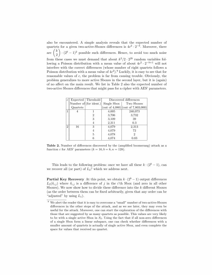
Due to the nature of the amplified attack, we do not need additional datato find all these values. They are just suggested by the different boomerangs.The only thing we need to take into account is that we want all k · (2b − 1)boomerangs to “succeed” (i.e., have enough quartets). In Table 2 we give anexample of parameters that follows AES’ ones (k = 16, b = 8, n = 128).

One additional technicality is the fact that there is some (non-zero) chancethat differential characteristics with two active Sboxes in the second-layer, may

8 We refer the interested reader to [2] for the full analysis, e.g., why there are c2 ·2n+2b

rather than c2/2 · 2n+2b quartets.

also be encountered. A simple analysis reveals that the expected number ofquartets for a given two-active-Sboxes differences is 4c2 · 2−b. Moreover, there

are

(k2

)· (2b − 1)2 possible such differences. Hence, to avoid too much noise

from these cases we must demand that about k2/2 · 22b random variables fol-lowing a Poisson distribution with a mean value of about 4c2 · 2−b+1 will notinterfere with the correct differences (whose number of right quartets follows aPoisson distribution with a mean value of 4c2).9 Luckily, it is easy to see that forreasonable values of c, the problem is far from causing trouble. Obviously, theproblem generalizes to more active Sboxes in the second layer, but it is (again)of no affect on the main result. We list in Table 2 also the expected number oftwo-active Sboxes differences that might pass for a cipher with AES’ parameters.

c Expected Threshold Discovered differencesNumber of (for ident.) Single Sbox Two SboxesQuartets (out of 4,080) (out of 7,803,000)

1 4 1 4,005 240,0732 3,706 3,7323 3,109 394 2,311 0.3

2 16 3 4,079 2,3134 4,079 725 4,078 26 4,074 0.03

Table 2. Number of differences discovered by the (amplified boomerang) attack as afunction c for AES’ parameters (k = 16, b = 8, n = 128).

This leads to the following problem: once we have all these k · (2b − 1), canwe recover all (or part) of L2? which we address next.

Partial Key Recovery At this point, we obtain k · (2b − 1) output differencesL2(δi,j) where δi,j is a difference of j in the i’th Sbox (and zero in all otherSboxes). We now show how to divide these difference into the k different Sboxes(as the order between them can be fixed arbitrarily, given that any order can be“adjusted” by using L1).

9 We alert the reader that it is easy to overcome a “small” number of two-active-Sboxesdifferences in the other steps of the attack, and as we see later, they may even beuseful for the attack. Moreover, one can start the exploration of the differences withthose that are suggested by as many quartets as possible. This values are very likelyto be with a single active Sbox in S2. Using the fact that if all non-zero differencesof a single Sbox form a linear subspace, one can check whether differences with asmaller amount of quartets is actually of single active Sbox, and even complete thespace for values that received no quartet.

The simplest method to do so, is to actually increase a bit the data/timecomplexity, and look for two active Sboxes in the second layer. It is easy to seethat once we identify all δi,j ’s values, then a difference in two active Sboxes canbe written as ∆ = δi,j ⊕ δi′,j′ , i.e., L2(∆) = L2(δi,j ⊕ δi′,j′) = L2(δi,j)⊕ (δi′,j′).This holds only when i 6= i′, and thus, we can identify when two of the oneactive Sbox differences do not share an Sbox (as there will be a correspondingtwo active Sbox difference for them). Hence, the separation into different Sboxescan be done quite immediately, resulting in an attack that requires c · 2n/2+3b/2

chosen plaintexts, and about the same amount of time.

4.3 Attacking the Full Structure

We now turn our attention to the full ASASA construction. The main problemwith directly applying the amplified boomerang attack to the full constructionis that we cannot have a difference in the first Sbox layer in only a single Sbox.

Luckily, the solution to the problem is to perform another birthday para-dox argument, and use a known-plaintext boomerang. The known-plaintextboomerang was first mentioned in [16], and its a natural extension of the boomerang(and the amplified boomerang attack). A random set of c·23n/4+b/2 known plain-texts, contains c2/2 · 23n/2+b pairs at the entrance to S0, i.e., offers c2/2 · 2n/2+bpairs with any given input difference, including those with a single active Sbox.As shown earlier, such amount of pairs is sufficient to generate right amplifiedboomerang quartets.

The only remaining task is the identification of the quartets ((P1, P2), (P3, P4))themselves. If both (P1, P2) and (P3, P4) are pairs which are part of the quar-tet, in other words, have the same difference in a single byte after L0 (i.e.,L0(P1 ⊕ P2) = L0(P3 ⊕ P4) with a single active Sbox), then P1 ⊕ P2 = P3 ⊕ P4.As before, we can also detect that L2(C1) ⊕ L2(C2) = L2(C3) ⊕ L2(C4). Thissuggests that finding the quartets ((P1, P2), (P3, P4)) can be easily done by:

– For all pairs of plaintext (Pi, Pj) store in a hash table Pi⊕Pj ||Ci⊕Cj (alongwith Pi and Pj).

– Collect all collisions in the table as candidate quartets, and analyze them asbefore.

Given c · 23n/4+b/2 known plaintexts, we expect c2/2 · 23n/2+b pairs, andin total c4/2 · 23n+2b quartets.10 Hence, we expect c4/2 · 2n+2b quartets to besuggested by the collisions in the table, out of which c4/2 are right quartets thatsuggest the correct differences in the plaintexts and in the ciphertexts. Thesedifferences are of course, differences that become an active single Sbox (eitherthrough L0 or the inverse of L2). Hence, once again, it is possible to identify allthe differences that are transformed into a single active Sbox (on both sides ofthe scheme). Again, increasing the data complexity a bit (to c ·23n/4+3b/4 known

10 We note that the quartet ((P1, P2), (P3, P4)) differs from the quartet((P1, P2), (P4, P3)).

plaintexts), allows finding all the differences that go to a single active Sbox, byworking with differences of two active Sboxes.

To conclude, one can easily identify the k · (2b − 1) differences that lead to asingle active Sbox thorough L0 or L2, using a known plaintext boomerang. Theattack takes c · 23n/4+3b/4 plaintexts, and has memory and time complexity ofc2/2 · 23n/2+3b/2.

5 Differential Attack: Using the DDT

We denote by

δ(α) := |{F (x) + F (x+ α) | x ∈ Fn2}|

the number of possible output differences for a given input difference.

The basic idea is that the number of possible output differences depends onthe number of active Sboxes in the first layer of Sboxes. More precisely, we relyon the following assumption.

Assumption 3 The number of possible output differences is (expected to be)smaller if only one Sbox is active in the first layer compared to the case whenmore than one Sbox is active in the first layer.

So the attack starts by computing δ(α) for all non-zero α values. This takes time22n and will be the bottleneck of the attack. Afterwards the list of all δ(α) issorted in increasing order. We denote the sorted list by T with T0 correspondingto α with the smallest δ(α) value.

The assumption is now that the top of the list contains mostly input-differencesα such that

L(α) = (β1, . . . , βk)

with only one βi ∈ Fb2 non-zero. In other words, the top of the list containsmainly elements α such that α ∈ Vi for some (unknown) 1 ≤ i ≤ k.

For recovering Vi we next have to sort those α values into different bins suchthat two α values are in the same bin iff they are both in the same subspace Vi.

We explain how to recover the first Vi, without loss of generality V0 , in detail.Recovering the remaining ones is very similar and will only be briefly sketched.

We start by considering the first t entries in the sorted table T . Choosing tsuch that

(tb

)is smaller than 22n makes sure that this step is not the bottleneck

of the attack. In most cases (as long as b ≤ 22k) it would be sufficient to chooset ≤ 22k, as (

22k

b

)≤(22k)b

= 22n.

However, our experiments show that the success probability of the attack isreduced for high values of t. The best results have been obtained when t was setto a small multiple of b.

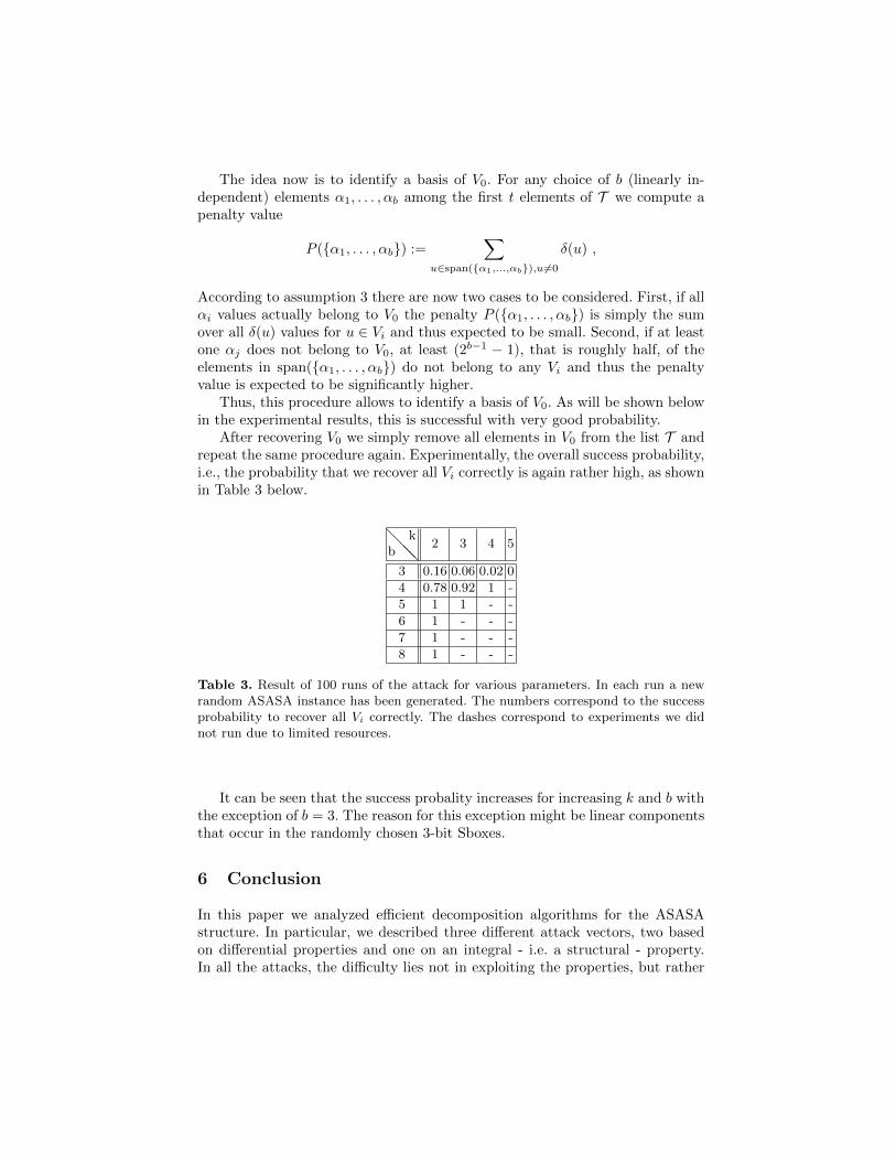
The idea now is to identify a basis of V0. For any choice of b (linearly in-dependent) elements α1, . . . , αb among the first t elements of T we compute apenalty value

P ({α1, . . . , αb}) :=∑

u∈span({α1,...,αb}),u6=0

δ(u) ,

According to assumption 3 there are now two cases to be considered. First, if allαi values actually belong to V0 the penalty P ({α1, . . . , αb}) is simply the sumover all δ(u) values for u ∈ Vi and thus expected to be small. Second, if at leastone αj does not belong to V0, at least (2b−1 − 1), that is roughly half, of theelements in span({α1, . . . , αb}) do not belong to any Vi and thus the penaltyvalue is expected to be significantly higher.

Thus, this procedure allows to identify a basis of V0. As will be shown belowin the experimental results, this is successful with very good probability.

After recovering V0 we simply remove all elements in V0 from the list T andrepeat the same procedure again. Experimentally, the overall success probability,i.e., the probability that we recover all Vi correctly is again rather high, as shownin Table 3 below.

@@@b

k2 3 4 5

3 0.16 0.06 0.02 0

4 0.78 0.92 1 -

5 1 1 - -

6 1 - - -

7 1 - - -

8 1 - - -

Table 3. Result of 100 runs of the attack for various parameters. In each run a newrandom ASASA instance has been generated. The numbers correspond to the successprobability to recover all Vi correctly. The dashes correspond to experiments we didnot run due to limited resources.

It can be seen that the success probality increases for increasing k and b withthe exception of b = 3. The reason for this exception might be linear componentsthat occur in the randomly chosen 3-bit Sboxes.

6 Conclusion

In this paper we analyzed efficient decomposition algorithms for the ASASAstructure. In particular, we described three different attack vectors, two basedon differential properties and one on an integral - i.e. a structural - property.In all the attacks, the difficulty lies not in exploiting the properties, but rather

in locating them as they are hidden by the external linear layers. Reciprocally,as soon as such a property has been detected, information on the linear layerscan be easily deduced, and combining the data gathered from several propertiesallows to peel off the external linear layers efficiently. While our integral attack isthe most efficient, it is not always applicable, and in such cases the other attacksshould be considered. Moreover, we feel that the boomerang and differentialattack vectors provide additional value, which could be further increased in thefuture if they are improved.

As our most efficient attacks have time complexity of roughly 23n/2, it seemsthat ASASA schemes must have a large block size n in order to be consideredas secure candidates for white-box cryptography. However, this requires theirblack-box representations to be extremely large and inappropriate for practicaluse (e.g., in order to guarantee a minimal security level of 64 bits, an ASASAscheme requires storage of about 243 words, which is more than 10 terabytes).A natural future work item is to study the security of general SP-networks withmore layers (e.g. ASASAS), and in particular, investigate if any of the attackspresented here can be generalized or improved on these constructions.

References

1. Eli Biham. Cryptanalysis of Patarin’s 2-Round Public Key System with S Boxes(2R). In Bart Preneel, editor, Advances in Cryptology - EUROCRYPT 2000, Inter-national Conference on the Theory and Application of Cryptographic Techniques,Bruges, Belgium, May 14-18, 2000, Proceeding, volume 1807 of Lecture Notes inComputer Science, pages 408–416. Springer, 2000.

2. Eli Biham, Orr Dunkelman, and Nathan Keller. The Rectangle Attack - Rectan-gling the Serpent. In Birgit Pfitzmann, editor, Advances in Cryptology - EURO-CRYPT 2001, International Conference on the Theory and Application of Crypto-graphic Techniques, Innsbruck, Austria, May 6-10, 2001, Proceeding, volume 2045of Lecture Notes in Computer Science, pages 340–357. Springer, 2001.

3. Alex Biryukov, Charles Bouillaguet, and Dmitry Khovratovich. CryptographicSchemes Based on the ASASA Structure: Black-Box, White-Box, and Public-Key(Extended Abstract). In Palash Sarkar and Tetsu Iwata, editors, Advances inCryptology - ASIACRYPT 2014 - 20th International Conference on the Theory andApplication of Cryptology and Information Security, Kaoshiung, Taiwan, R.O.C.,December 7-11, 2014. Proceedings, Part I, volume 8873 of Lecture Notes in Com-puter Science, pages 63–84. Springer, 2014.

4. Alex Biryukov and Adi Shamir. Structural Cryptanalysis of SASAS. J. Cryptology,23(4):505–518, 2010.

5. Julia Borghoff, Lars R. Knudsen, Gregor Leander, and Søren S. Thomsen. Slender-Set Differential Cryptanalysis. J. Cryptology, 26(1):11–38, 2013.

6. Christina Boura and Anne Canteaut. On the Influence of the Algebraic Degree of

F-1 on the Algebraic Degree of G ◦ F. IEEE Transactions on Information Theory,59(1):691–702, 2013.

7. Joan Daemen, Lars R. Knudsen, and Vincent Rijmen. The Block Cipher Square.In Eli Biham, editor, Fast Software Encryption, 4th International Workshop, FSE’97, Haifa, Israel, January 20-22, 1997, Proceedings, volume 1267 of Lecture Notesin Computer Science, pages 149–165. Springer, 1997.

8. Henri Gilbert, Jerome Plut, and Joana Treger. Key-Recovery Attack on the ASASACryptosystem with Expanding S-boxes. In CRYPTO 2015, Lecture Notes in Com-puter Science. Springer, 2015. to appear.

9. John Kelsey, Tadayoshi Kohno, and Bruce Schneier. Amplified Boomerang AttacksAgainst Reduced-Round MARS and Serpent. In Bruce Schneier, editor, Fast Soft-ware Encryption, 7th International Workshop, FSE 2000, New York, NY, USA,April 10-12, 2000, Proceedings, volume 1978 of Lecture Notes in Computer Science,pages 75–93. Springer, 2000.

10. Lars R. Knudsen. Truncated and Higher Order Differentials. In Bart Preneel, ed-itor, Fast Software Encryption: Second International Workshop. Leuven, Belgium,14-16 December 1994, Proceedings, volume 1008 of Lecture Notes in ComputerScience, pages 196–211. Springer, 1994.

11. Lars R. Knudsen and David Wagner. Integral Cryptanalysis. In Joan Daemen andVincent Rijmen, editors, Fast Software Encryption, 9th International Workshop,FSE 2002, Leuven, Belgium, February 4-6, 2002, Revised Papers, volume 2365 ofLecture Notes in Computer Science, pages 112–127. Springer, 2002.

12. Xuejia Lai. Higher Order Derivatives and Differential Cryptanalysis. In ”Sympo-sium on Communication, Coding and Cryptography”, in honor of James L. Masseyon the occasion of his 60’th birthday, pages 227–233, 1994.

13. Luke O’Connor. On the Distribution of Characteristics in Bijective Mappings. J.Cryptology, 8(2):67–86, 1995.

14. Jacques Patarin and Louis Goubin. Asymmetric cryptography with S-Boxes. InYongfei Han, Tatsuaki Okamoto, and Sihan Qing, editors, Information and Com-munication Security, First International Conference, ICICS’97, Beijing, China,November 11-14, 1997, Proceedings, volume 1334 of Lecture Notes in ComputerScience, pages 369–380. Springer, 1997.

15. Tyge Tiessen, Lars R. Knudsen, Stefan Kolbl, and Martin M. Lauridsen. Securityof the AES with a Secret S-box. In FSE 2015, Lecture Notes in Computer Science.Springer, 2015. to appear.

16. David Wagner. The Boomerang Attack. In Lars R. Knudsen, editor, Fast Soft-ware Encryption, 6th International Workshop, FSE ’99, Rome, Italy, March 24-26,1999, Proceedings, volume 1636 of Lecture Notes in Computer Science, pages 156–170. Springer, 1999.