Embed Size (px)
Citation preview
Decomposing the co-movement of the business cycle:a time-frequency analysis of growth cycles in the
eurozone�
Patrick M. Crowleyy and Jim Leez
March 2005
Abstract
This article analyses the frequency components of European business cycles usingreal GDP by employing multiresolution decomposition (MRD) with the use of max-imal overlap discrete wavelet transforms (MODWT). Static wavelet variance andcorrelation analysis is performed, and phasing is studied using co-correlation with theeurozone by scale. Lastly dynamic conditional correlation GARCH models are used toobtain dynamic correlation estimates by scale against the EU to evaluate synchronic-ity of cycles through time. The general �ndings are that eurozone members fall intoone of three categories: i) high static and dynamic correlations at all frequency cy-cles (e.g. France, Belgium, Germany), ii) low static and dynamic correlations, withlittle sign of convergence occurring (e.g. Greece), and iii) low static correlation butconvergent dynamic correlations (e.g. Finland and Ireland).Keywords: Business cycles, growth cycles, European Union, multiresolution
analysis, wavelets, co-correlation, dynamic correlation.JEL Classi�cation: C65, E32, O52
Acknowledgements: The Bank of Finland are to be thanked for their hospitalityfor Crowley during the 2004/05 academic year. Able research assistance was providedby Helinä Laakkonen, Emmi Martikainen and Tarja Yrjölä.
�Disclaimer: the views expressed in this paper are those of the authors, and do not re�ect the views ofthe Bank of Finland.
yResearch department, Bank of Finland, Helsinki, Finland and College of Business, Texas A&M Uni-versity, Corpus Christi, TX, USA.
zCollege of Business, Texas A&M University, Corpus Christi, TX, USA.
1
Eurozone business cycles
1 Introduction
All economies experience business cycles, and since the Second World War these cycles
have been getting longer, but nonetheless, despite the occasional optimistic forecast that
the phenomenon no longer exists1, the cycle of economic expansion followed by recession
persists. There is a long-standing interest in macroeconomics in the nature and origins
of business cycles and, judging by certain undergraduate macroeconomics textbooks, some
macroeconomists would maintain that macroeconomics and the study of the business cycle
are mutually inclusive endevours. The causes of the business cycle are still largely a mys-
tery in economics and for many constitute the sole raison d�être for a macroeconomist -
indeed one of the major criticisms of mainstream economics2 is that much of the focus in
macroeconomics has moved away from trying to understand business cycles.to more tech-
nical aspects of models and econometrics. Nonetheless, over the last 15 years, with the
introduction of real business cycle models into the mainstream literature, there has been a
resurgence of interest in business cycles and what causes them.
Research on business cycles can be grouped into three di¤erent but overlapping strands
- one strand looks at historical business cycles to try and ascertain the important factors
driving the business cycle (and those that therefore should underpin any model), another
strand looks at the international co-movement of business cycles, and the third strand looks
at asymmetries in the business cycle itself. The original approach to business cycle research
was made in the early part of the last century, and sought to uncover "stylized facts" by
constructing datasets that are as long and as internationally broad as possible. This strand
had its origins in early work done as far back as the 1920s by economists such as Kitchin
(1923), Mitchell (1946), Kuznets (1958), and more recently Lucas (1977). The approach
is particularly important for construction of theoretical models of the business cycle, as if
they are to be relevant, models must replicate whatever regularities are observed in the
data. This �rst strand of the literature is probably best summed up by Basu and Taylor
(1999) who search for regularities in business cycles over more than a century of data from 18
countries. To motivate the second strand, one of the most noticeable trends of the 1980s and
1990s was the increasing regionalisation of the world economy along the line of trading blocs,
and so in recognition of the fact that the likelihood of simultaneous economic downturns
1For example, to quote Rudiger Dornbusch in 1998, �Not to worry, this expansion will run forever; . . .A slowdown is purely possible as is stock market correction, but not an old-fashioned recession; at most abanana�.
2Such as those made by the Austrian School (see Garrison (2001) for example).
Crowley and Lee Page: 2
Eurozone business cycles
should be higher within a given regional trading block, economists started looking at the co-
movement of business cycles across countries (see Backus and Kehoe (1992) for perhaps the
seminal article here). The last strand of the literature perhaps probably had its genesis with
Keynes (1936) but its latest variation began with Sichel (1993), who de�ned an asymmetric
business cycle as "one in which some phase of the cycle is di¤erent from the mirror image
of the opposite phase, so that contractions might be steeper, on average, than expansions".
In this strand the advances in econometric methodology probably spurred the revival in
interest in business cycles after the publication of the Hamilton (1989) Markov-switching
model.
This paper is mainly concerned with the second strand of the business cycle literature
referred to above, relating to the co-movement of business cycles, but it also takes in some
of the concerns of the other strands as well. It takes a new unique approach, using new
techniques in time-frequency analysis developed in the signal processing �eld of engineering
to identify di¤erent periodicity cycles in real GDP. These cycles are then correlated at
their various periodicities and then the dynamics of the cycle phases over time at these
periodicities are studied.
The following section gives a brief review of the business cycle literature relating to the
EU, then section 3 provides a very brief description of time-frequency analysis. Section 4
provides results for a static variance and correlation analysis of real GDP cycles using the
wavelet approach while section 5 then explains and applies a dynamic correlation approach
to the same data. Section 6 concludes and suggests further research.
2 A brief review of EU business cycle research
2.1 The co-movement of business cycles
As A�Hearn and Woitek (2001) note, Morgenstern (1959) was probably the �rst economist
to observe and measure the comovement in business cycles on an international level. This
observation was again picked up in the more recent literature by Backus and Kehoe (1992)
and Backus, Kehoe, and Kydland (1992), who constructed a real business cycle model to
examine how cyclical variations in output and other aggregates were correlated across coun-
tries. From their model, because of asymmetric supply shocks, they anticipated negative
cross-correlation between output between countries, but in fact found quite strong positive
correlations. Because of risk sharing giving rise to promotion of consumption smoothing,
they expected quite high cross-correlations of consumption, but found only moderately high
Crowley and Lee Page: 3
Eurozone business cycles
cross correlations. They also anticipated negative cross-correlations between investment
and employment across countries (as asymmetric shocks cause capital �ows between coun-
tries), and yet again found quite strongly positive correlations. These apparant anomolies
are extensively discussed in Backus, Kehoe, and Kydland (1995), and since have become
known in the literature as the quantity anomoly3.
One criticism of this approach has been made by Canova and de Nicoló (2003), who
point out that the models of the type used by Backus, Kehoe, and Kydland (1992) rely
on temporary supply shocks to create the business cycles, and yet Canova and de Nicolo
�nd that demand shocks are the most important source of output �uctuation. Canova
and de Nicoló (2003) also found that structural disturbances appear uncorrelated across
countries, with the exception of the US and Canada, and yet these types of disturbance have
a key role in driving the business cycle in real business cycle models. Duarte and Holden
(2003) took a slightly di¤erent approach by looking at the cyclical and trend components
of real GDP for the G7 countries using various econometric speci�cations, to try and �nd
similarities and di¤erences, particularly in the cyclical components. They found that from
around 1990 two separate cycles seem to be developing �one for the US, Canada, and the
UK and the other for Germany, Italy, and France.
More recent research by Ambler, Cardia, and Zimmerman (2004) replicates the Backus
et al results with a much larger dataset using a GMM methodology and notes that i) em-
pirically, productivity correlations are greater than output correlations which in turn are
greater than consumption correlations, and ii) that the empirical results tend not to support
theoretical models that predict that comovements should either be negative (investment,
output and employment) or high and positive (consumption). Clearly the inference from
these results is that the underlying causes of business cycles needs to be better under-
stood empirically, before theoretical models can properly �ll in the modes and methods of
transmission.
In an attempt to �ll in these empirical gaps Baxter and Kouparitsas (2004) take a
somewhat di¤erent approach to comovement in business cycles by noting that the main
candidates for the comovement observation are trade4, industrial structure5, factor endow-
3This label appears to be somewhat of a misnomer, as there is little connection to quantities in aneconomics sense in their observation, and something is usually de�ned as anomolous if it is " a deviationor departure from the normal or common order, form, or rule". What was observed is probably betterlabelled an ordering reversal !
4See Frankel and Rose (2002)5See Helpman and Krugman (1985)
Crowley and Lee Page: 4
Eurozone business cycles
ments6, and gravity variables7. Using Leamer�s "extreme bounds analysis" (see Leamer
(1983)) so that measurement error can be taken into account.( - called robustness analysis),
they �nd that higher bilateral trade is correlated with higher business cycle correlation, as
is the stage of development of both countries and the distance between the two countries.
Other variables (such as greater similarity in industrial structure belonging to a currency
union and factor endowments) which have been thought to have an in�uence on business
cycles in the literature, were all found to be fragile.
2.2 EU Business cycle research
The creation of a single currency area in Europe has prompted in a lot of business cycle
research focused on the eurozone and the European Union. Studies by Artis and Zhang
(1997), Artis and Zhang (1999) and Sensier, Artis, Osborn, and Birchenhall (2004) establish
that since the inception of the exchange rate mechanism (ERM) of the European Monetary
System (EMS), business cycles in the European Union have been on a convergent trend.
This is an important issue, as economic theory doesn�t o¤er any de�nitive guidance as to
whether shocks should become more symmetric and cycles more synchronous. As Altavilla
(2004) notes, one view maintains that monetary union, through increasing trade intensity,
and co-committant economic and �nancial integration would yield both less asymmetric
shock propogation and also greater business cycle synchronization. The other view, which
stems from work by Krugman (1991), states that agglomeration e¤ects would create more
asymmetric shocks and therefore cause business cycles to be less synchronous. Indeed,
although studies which stress the propagation of shocks tend to show that the former
view dominates, those that put more emphasis on the synchronicity of business cycles
(for example, De Haan, Inklaar, and Sleijpen (2002)) tend not to show a great degree of
synchronicity in cycles between EU member states. Altavilla (2004) extends results by
Agresti and Mojon (2001) using a variety of methodologies, mainly sourced from articles by
James Hamilton (for example, Hamilton (1989)) and Harding and Pagan (see for example
Harding and A. (2002)), and �nds that although turning points for eurozone member states
were similar, the time-path of output between these points was less so (but dependent on the
�ltering technique used). The average duration of the EU business cycle was calculated
at around 3 years, which was equivalent in length to that of the US. In addition tests
6Standard trade theory (Ricardian and Heckscher-Ohlin, for example) would predict that this wouldin�uence the business cycle.
7Variables such as whether two countries are members of a currency union, the distance between thetwo countries, and at what stage in their development the two countries are, etc.
Crowley and Lee Page: 5
Eurozone business cycles
for synchronicity against the EU business cycle showed that although for some eurozone
countries (notably Spain and Italy) this was quite low, but Germany, Belgium and France
(in roughly that order) tended to have the strongest degrees of synchronization against the
EU business cycle.
A completely di¤erent approach to EU business cycles originated in work done by
Granger (1966)8 and has been continued by those such as Croux, Forni, and Reichlin
(2001), Valle e Azevedo (2002) and Levy and Dezhbakhsh (2003a), who use spectral analy-
sis to study the properties of business cycle variables in the frequency domain. Croux,
Forni, and Reichlin (2001) derive a measure of dynamic correlation which they label "co-
hesion"9 for log di¤erenced annual measures of GDP for European countries and annual
personal income for the US states and Federal Reserve regions from 1962-97, and �nd that
as expected, the US regions or states are far more cohesive than Europe, but that eurozone
member states are a little more cohesive than the EU taken as a whole. They claim to
identify the business cycle frequency as approximately 4 years in both cases, and �nd that
cohesion at this frequency is at its highest for the US but this is not the case for the EU. In
another paper in this strand, Valle e Azevedo (2002), using annual data from 1960-99, �nds
that the modal duration of the business cycle is about 9.25 years and the mean duration is
8.79 years. Using a co-spectrum, he goes on to estimate the dynamic correlation for each
country vs the EU11, and arrives at high correlations for France and Germany, middling
correlations for Italy and Spain and low correlations for other countries ( - Finland, Sweden,
UK and USA). Although the dynamic correlation results appear to be qualitatively similar
between the two studies, note that the estimate of the business cycle duration in the study
by Valle e Azevedo (2002) was signi�cantly di¤erent from that obtained by Croux, Forni,
and Reichlin (2001). Levy and Dezhbakhsh (2003a) estimate the output growth rate spec-
tra for a group of 58 countries using both annual and quarterly data, and �nd that these
spectra signi�cantly between countries, but they �nd that for most of the OECD countries
the mass of the spectrum lies in the business cycle frequency band (estimated at between
12 and 32 quarters). But in their results for quarterly data there are many exceptions10,
and for middle-developed and lesser-developed countries this general assertion about the
location of the mass of the spectra is not true at all.
8Updated by Levy and Dezhbakhsh (2003b) for a variety of countries.9In the paper they show that their measure at zero frequency is equivalent to the notion of stochastic
co-integration.10Those countries where the mass of the spectrum was located in i) longer cycles - Canada, Austria
and Japan; ii) business cycles - Switzerland, France, UK, Finland; and iii) shorter cycles - US, Australia,Sweden, Denmark, Netherlands, Austria.
Crowley and Lee Page: 6
Eurozone business cycles
The traditional view, embodied in the work of Bergman, Bordo, and Jonung (1998)
is that the business cycle lasts for 4.8 years on average during the post-war period, with
countries like Finland having longer average cycles (5.8 years) and countries such as Norway
having shorter cycles (3.6 years)11. Clearly di¤erent studies use di¤erent datasets, and
di¤erent methodologies select di¤erent business cycle lengths in the data, and perhaps one
could posit the existence of cycles occurring at di¤erent medium term frequencies12, as
mirrored in the approach taken by Comin and Gertler (2003) where they look for cycles in
macroeconomic data in two frequency bands: from 2 to 32 quarters (0.5 to 8 years) and
from 32 to 200 quarters (8 to 50 years), over the period from 1948 to 2001. Although their
results and model focus on the longer medium term cycles, they suggest a considerably
higher variance for these medium term cycles, and attach much greater importance to this
cycle.
3 Multiresolution analysis
3.1 Why wavelets?
In all the research done to date on business cycles, it is has been impossible to satisfactorily
simultaneously separate out di¤erent frequencies in output data so as to identify cycles in
the time domain at di¤erent frequencies. Traditionally, spectral analysis su¤ers from the
problem of its inability to deal with time-varying cycles, lack of regularity in the business
cycle, and reliance on stationary data and therefore the usage of appropriate detrending
methods. Thus the work horse of spectral analysis, namely the Fourier transform and its
variants, has not always yielded interesting results when applied to actual economic data,
as the Fourier method assumes that series are homogeneous in their characteristics, so that
periodicity is regular and no shocks or other exogenous events exist. Further, any shift in
periodicities would appear as peaks in the spectrum at two di¤erent frequencies, when in
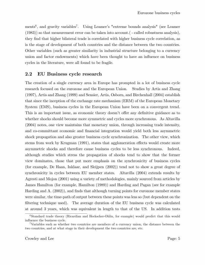
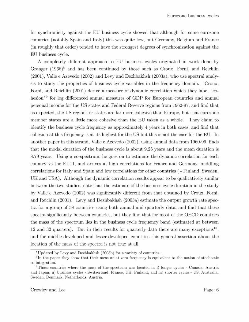
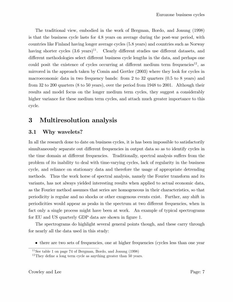
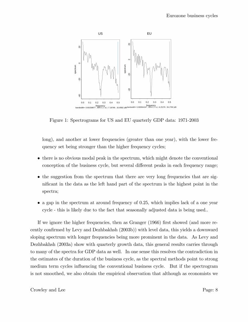
fact only a single process might have been at work. An example of typical spectrograms
for EU and US quarterly GDP data are shown in �gure 1.
The spectrograms do highlight several general points though, and these carry through
for nearly all the data used in this study:
� there are two sets of frequencies, one at higher frequencies (cycles less than one year11See table 1 on page 74 of Bergman, Bordo, and Jonung (1998)12They de�ne a long term cycle as anything greater than 50 years.
Crowley and Lee Page: 7
Eurozone business cycles
0.0 0.1 0.2 0.3 0.4 0.5frequency
40
20
020
spec
trum
bandwidth= 0.000964347 , 95% C.I. is ( 8.25378 , 56.2789 )dB
EU
0.0 0.1 0.2 0.3 0.4 0.5frequency
40
20
020
spec
trum
US
bandwidth= 0.00158877 , 95% C.I. is ( 7.19769 , 32.9582 )dB
Figure 1: Spectrograms for US and EU quarterly GDP data: 1971-2003
long), and another at lower frequencies (greater than one year), with the lower fre-
quency set being stronger than the higher frequency cycles;
� there is no obvious modal peak in the spectrum, which might denote the conventionalconception of the business cycle, but several di¤erent peaks in each frequency range;
� the suggestion from the spectrum that there are very long frequencies that are sig-
ni�cant in the data as the left hand part of the spectrum is the highest point in the
spectra;
� a gap in the spectrum at around frequency of 0.25, which implies lack of a one year
cycle - this is likely due to the fact that seasonally adjusted data is being used..
If we ignore the higher frequencies, then as Granger (1966) �rst showed (and more re-
cently con�rmed by Levy and Dezhbakhsh (2003b)) with level data, this yields a downward
sloping spectrum with longer frequencies being more prominent in the data. As Levy and
Dezhbakhsh (2003a) show with quarterly growth data, this general results carries through
to many of the spectra for GDP data as well. In one sense this resolves the contradiction in
the estimates of the duration of the business cycle, as the spectral methods point to strong
medium term cycles in�uencing the conventional business cycle. But if the spectrogram
is not smoothed, we also obtain the empirical observation that although as economists we
Crowley and Lee Page: 8
Eurozone business cycles
measure the business cycle in terms of when recessions occur, the GDP series suggests that
there are potentially many other cycles with di¤erent periodicities at work in the data13.
Of course the business cycle itself has various phases, as Kontolemis (1997) makes clear, but
if they are of the four phase variety originally described by Hicks (1950), then they could
occur at di¤erent frequencies to the business cycle itself, given that accelerating and de-
celerating growth cycles might not be in concordance with the conventional business cycle.
Zarnovitz (1985) �rst suggested that these more frequent "growth cycles" might have an
important role to play in the business cycle itself, and set about studying them. In terms
of dating these growth cycles, Zarnowitz and Ozyildirim (2002) conduct various time series
decomposition approaches to identify the cycles, and construct a "growth cycle" chronology
for the US.
Wavelet analysis sets itself apart from both the frequency and time domain approaches
by combining elements of both14. Wavelets have the ability to decompose a series into
various frequency components, albeit with constraints on how these frequencies are de�ned,
at any given point in time. They therefore can be categorised as time-frequency analysis.
The advantages of using wavelets to analyse business cycles are immediately clear: unlike
frequency domain analysis, they can identify which frequencies are present in the data at
any given point in time. Once a series has been decomposed into these di¤erent frequencies,
time series can then be extracted for further analysis.
Only one previous contribution to the business cycle literature has been made using
wavelet analysis, that of Crivellini, Gallegati, Gallegati, and Palestrini (2004). They use
industrial production data for several EU countries, and decompose the data into di¤er-
ent frequencies and then analyse each di¤erent frequency separately in terms of duration,
amplitude, phasing and possible cause. The approach taken here is complementary to
their study, but the focus is instead on the co-movement of growth cycles in the EU using
quarterly data.
3.2 Data
The data in this study was provided by the Bank of Finland, which in turn was sourced
from the OECD with the exception of the US data (which was obtained from the US
13So as not to confuse the generally accepted notion of a business cycle with also the more generalde�nition of a medium term cycle used by Comin and Gertler (2003), from this point onwards the term"growth cycles" is used to describe cycles at di¤erent frequencies present in GDP growth data.14Crowley (2005) provides a comprehensive overview of wavelets and reviews existing and potential
applications in the economics literature.
Crowley and Lee Page: 9
Eurozone business cycles
Bureau of Economic Analysis) and the Swiss data ( - which was obtained from the Bank
for International Settlements)15. The eurozone (EU12) aggregate was sourced from the
ECB�s euro area wide model (AWM)16. The data frequency is quarterly, the span is from
1970-2004Q2 and the data is seasonally adjusted17. So as to identify growth cycles, the data
is annually log-di¤erenced, which should then also neutralise any di¤erences in methods of
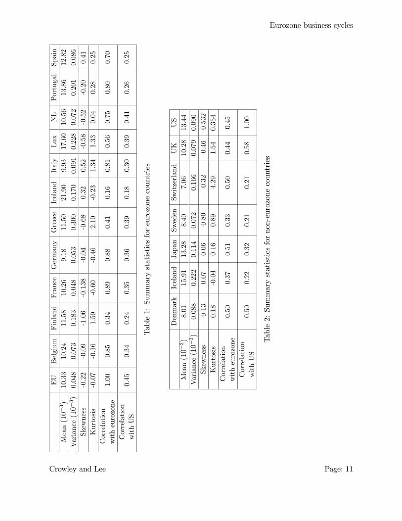
seasonal adjustment. Summary statistics for the log-di¤erenced GDP data are presented
in table 1 and 2, including basic Pearson correlations with the eurozone GDP growth data
and with the US growth data.
15In all cases sourced data are seasonally adjusted, with the exception of Switzerland, where the sourcedSwiss data was seasonally adjusted by the Bank of Finland using the STAMP program. Adjustments werealso made to the German data to eliminate the "jump" in the data after reuni�cation in 1991.16See Fagan, Henry, and Mestre (2001).17Seasonal adjustment in business cycle studies continues to be controversial as Mir and Osborn (2004)
show. The analysis here was repeated for several seasonally adjusted series, and only small di¤erenceswere apparent.
Crowley and Lee Page: 10
Eurozone business cycles
EU
Belgium
Finland
France
Germany
Greece
Ireland
Italy
Lux
NL
PortugalSpain
Mean(10�
3)
10.33
10.24
11.58
10.26
9.18
11.50
21.90
9.93
17.60
10.56
13.86
12.82
Variance(10�
3)
0.048
0.073
0.183
0.048
0.053
0.300
0.170
0.091
0.228
0.072
0.201
0.086
Skewness
-0.22
-0.09
-1.06
-0.138
-0.04
-0.68
0.32
0.52
-0.58
-0.52
-0.20
0.41
Kurtosis
-0.07
-0.16
1.59
-0.60
-0.46
2.10
-0.23
1.34
1.33
0.04
0.28
0.25
Correlation
witheurozone
1.00
0.85
0.34
0.89
0.88
0.41
0.16
0.81
0.56
0.75
0.80
0.70
Correlation
withUS
0.45
0.34
0.24
0.35
0.36
0.39
0.18
0.30
0.39
0.41
0.26
0.25
Table1:Summarystatisticsforeurozonecountries
Denmark
Iceland
Japan
Sweden
Switzerland
UK
US
Mean(10�
3)
8.01
15.91
13.28
8.40
7.06
10.28
13.44
Variance(10�
3)
0.088
0.222
0.114
0.072
0.166
0.079
0.090
Skewness
-0.13
0.07
0.06
-0.80
-0.32
-0.46
-0.532
Kurtosis
0.18
-0.04
0.16
0.89
4.29
1.54
0.354
Correlation
witheurozone
0.50
0.37
0.51
0.33
0.50
0.44
0.45
Correlation
withUS
0.50
0.22
0.32
0.21
0.21
0.58
1.00
Table2:Summarystatisticsfornon-eurozonecountries
Crowley and Lee Page: 11
Eurozone business cycles
In table 1, unsurprisingly, the member states that were previously known as the "hard
core" of EMU member states (France, Germany, Belgium, Luxembourg and the Nether-
lands) all have high correlations against the eurozone18, but interestingly Italy and Portugal
also now appear to have relatively high correlations against the eurozone. The low corre-
lations for Finland, Greece and Ireland must give some cause for concern for policymakers,
particularly as all of these member states are on the periphery of the EU. In table 2 for the
non-eurozone countries, all of the correlations with the eurozone are relatively low but all
positive, and interestingly for both Denmark and the UK, two countries with opt-outs from
EMU, correlations with the US are greater or equal to those with the eurozone. These
simple correlations though are in line with previous studies with respect to the groupings
of countries before the inception of EMU.
3.3 Basic wavelets
Wavelets are a relatively recent innovation in mathematics and originally stem from research
by Mallat (1989) and Debauchies (1992). The main feature of wavelet analysis is that
it enables the researcher to separate a variable or signal into its constituent frequency
components. Consider a double sequence of functions:
(t) =1ps
�t� u
s
�(1)
where s is a sequence of scales, where scale here corresponds to a particular frequency
range. The term 1psensures that the norm of (:) is equal to one. The function (:)
is then centered at u with scale s. In the language of wavelets, the energy of (:) is
concentrated in a neighbourhood of u with size proportional to s, so that as s increases
the length of support in terms of t increases For example, when u = 0, the support of
(:) for s = 1 is [d;�d]. As s is increased, the support widens to [sd;�sd]. Dilation (i.e.changing the scale) is particularly useful in the time domain, as the choice of scale indicates
the "stretching" used to represent any given variable or signal. A broad support wavelet
yields information on variable or signal variations on a large scale, whereas a small support
wavelet yields information on signal variations on a small scale. The important point here
is that as projections are orthogonal, wavelets at a given scale are not a¤ected by features
of a signal at scales that require narrower support. Lastly, if a wavelet is shifted on the
time line, this is referred to as translation or shift of u. Any series x(t) can be built up
18With the exception of Luxembourg.
Crowley and Lee Page: 12
Eurozone business cycles
as a sequence of projections onto father and mother wavelets indexed by both j; the scale,
and k, the number of translations of the wavelet, where k is often assumed to be dyadic.
As shown in Bruce and Gao (1996), if the wavelet coe¢ cients are approximately given by
the integrals:
sJ;k �Zx(t)�J;k(t)dt (2)
dj;k �Zx(t) j;k(t)dt (3)
j = 1; 2; :::J such that J is the maximum scale sustainable with the data to hand, then a
multiresolution representation of the signal x(t) is can be given by:
x(t) =Xk
sJ;k�J;k(t) +Xk
dJ;k J;k(t) +Xk
dJ�1;k J�1;k(t) + :::+Xk
d1;k 1;k(t) (4)
where the basis functions �J;k(t) and J;k(t) are assumed to be orthogonal, that is:R�J;k(t)�J;k0 (t) = �k;k0R J;k(t)�J;k0 (t) = 0R
J;k(t) J 0 ;k0 (t) = �k;k0�j;j0(5)
where �i;j = 1 if i = j and �i;j = 1 if i 6= j. Note that when the number of observations is
dyadic, the number of coe¢ cients of each type is given by:
� at the �nest scale 21 :there are n2coe¢ cients labelled d1;k.
� at the next scale 22 :there are n22coe¢ cients labelled d2;k.
� at the coarsest scale 2J :there are n2Jcoe¢ cients dJ;k and SJ;k
In wavelet language, each of these coe¢ cients is called an "atom" and the set of coef-
�cients for each scale are termed "crystals"19. The multiresolution decomposition (MRD)
of the variable or signal x(t) is then given by the set of crystals:
fSJ ; DJ ; DJ�1; :::D1g (6)
The interpretation of the MRD using the DWT is of interest as it relates to the frequency
at which activity in the time series occurs. For example with a quarterly time series table
3 shows the frequencies captured by each scale crystal:
19Hence the atoms make up the crystal for each scale of the wavelet resolution.
Crowley and Lee Page: 13
Eurozone business cycles
Scalecrystals
Quarterlyfrequencyresolution
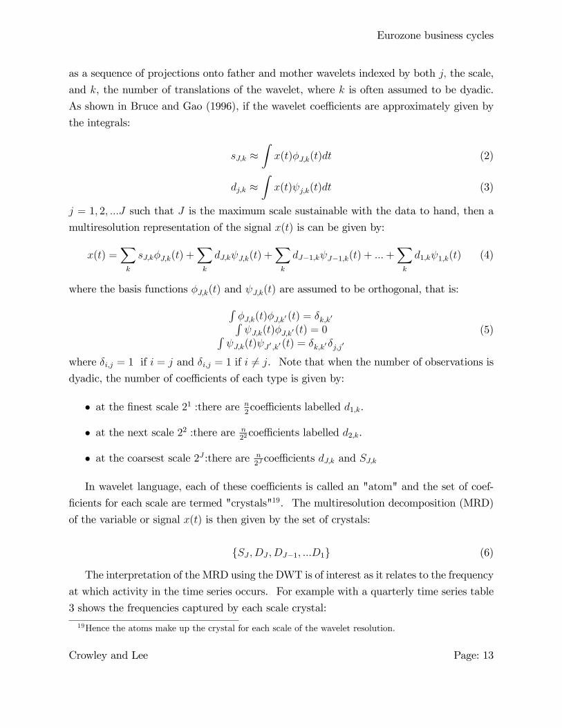
d1 1-2d2 2-4d3 4-8=1-2yrsd4 8-16=2-4yrsd5 16-32=4-8ysd6 64-128=8-16yrsd7 128-256=16-32yrsd8 etc
Table 3: Frequency interpretation of MRD scale levels
Note that as quarterly data is used in this study, to capture the conventional business
cycle length scale crystals need to be obtained for 5 scales. This requires at least 64
observations, but as we have 132 observations this is easily accomplished20. The data
are transformed into year over year changes in log real GDP. It should be noted at this
juncture, that if conventional business cycles are usually assumed to range from 12 quarters
(3 years) to 32 quarters (8 years)21, then crystals d4 and d5 will be assumed to contain
business cycle frequencies.
3.4 MODWT
In the wavelet literature there are various methods that can be used for decomposing a
series or signal. The �rst transform to be used extensively in applications was the Discrete
Wavelet Transform (DWT). Although extremely popular due to its intuitive approach,
the DWT su¤ers from two drawbacks: dyadic length requirements for the series to be
transformed and the fact that the DWT is non-shift invariant. In order to address these
two drawbacks, the maximal-overlap DWT (MODWT)22 was introduced by ?) and a phase-corrected version was introduced and was compared and found superior to other methods
20A preliminary version of this paper used 6 scales, but has been dropped in this version of the paper,as for virtually all countries, the 6th scale carries very little energy.21Given our discussion above, and as assumed by Levy and Dezhbakhsh (2003a), when evaluating output
growth rate spectra.22As Percival and Walden (2000) note, the MODWT is also commonly referred to by various other
names in the wavelet literature such as non-decimated DWT, time-invariant DWT, undecimated DWT,translation-invariant DWT and stationary DWT. The term "maximal overlap" comes from its relationshipwith the literature on the Allan variance (the variation of time-keeping by atomic clocks) - see Greenhall(1991).
Crowley and Lee Page: 14
Eurozone business cycles
of frequency decomposition23 by ?). The MODWT gives up the orthogonality property ofthe DWT to gain other features, given in Percival and Mofjeld (1997) as:
� the ability to handle any sample size regardless of whether the series is dyadic or not;
� increased resolution at coarser scales as the MODWT oversamples the data;
� translation-invariance - in other words the MODWT crystal coe¢ cients do not changeif the time series is shifted in a "circular" fashion; and
� the MODWT produces a more asymptotically e¢ cient wavelet variance estimator
than the DWT.
Both Gençay, Selçuk, and Whicher (2001) and Percival and Walden (2000) give a thor-
ough and accessible description of the MODWT using matrix algebra. With time series,
one of the problems in using the MODWT is that the calculations of crystals occurs at
roughly half the length of the wavelet basis into the series at any given scale. Thus the
crystal coe¢ cients start further and further along the time axis as the scale level increases.
As the MODWT is shift invariant, the MRD will not change with a circular shift in the
time series, so that each scale crystal can be appropriately shifted so that the coe¢ cients
line up with the original data. This is done by lagging the crystals by increasingly large
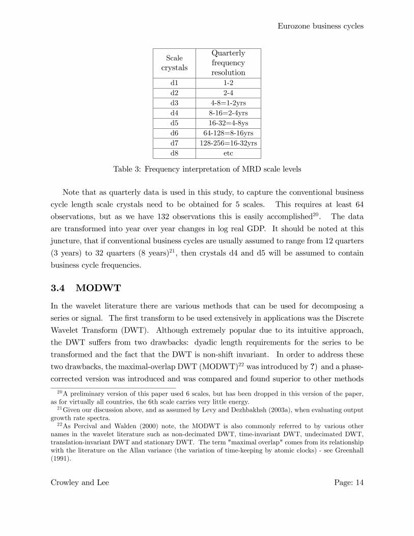
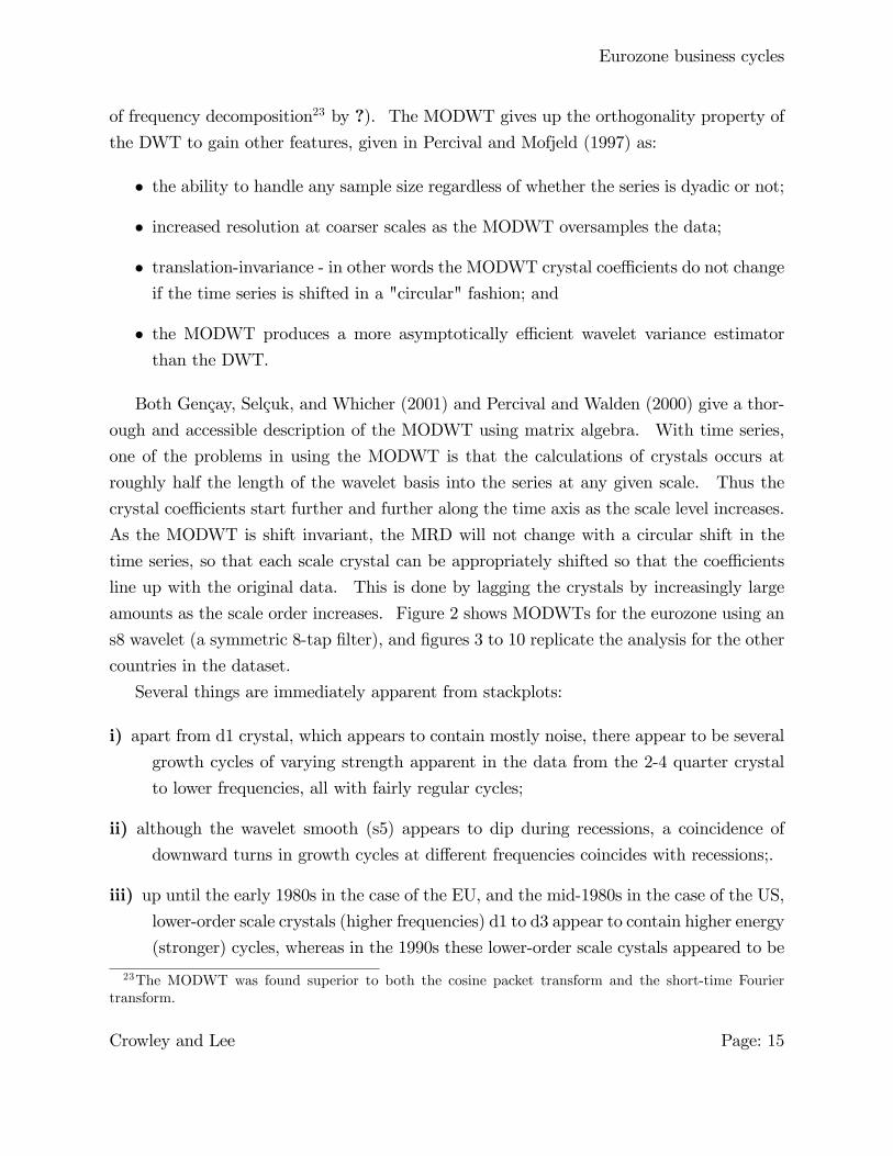
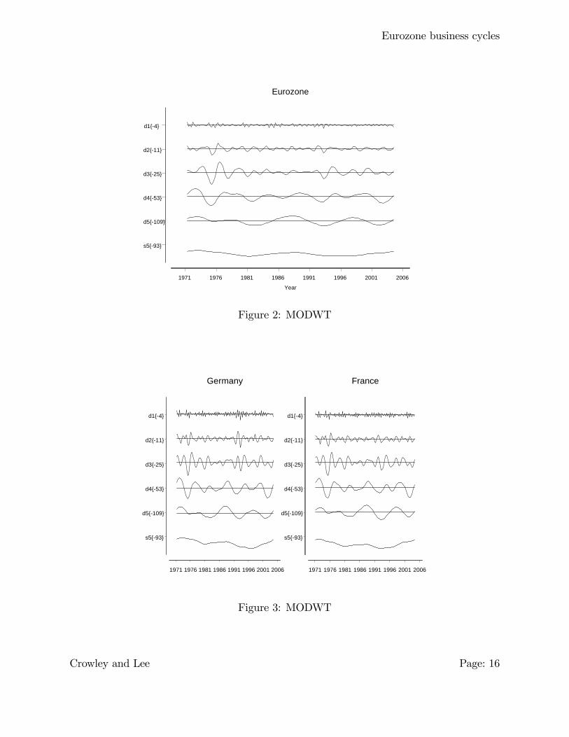
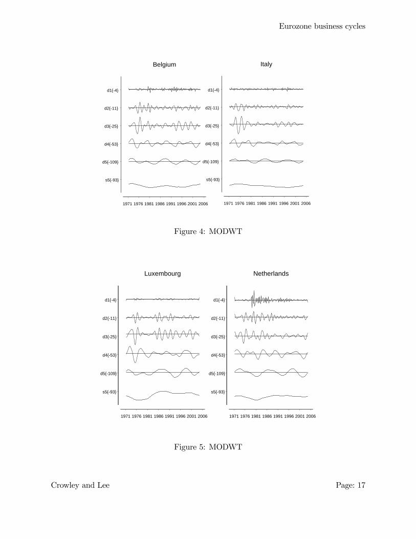
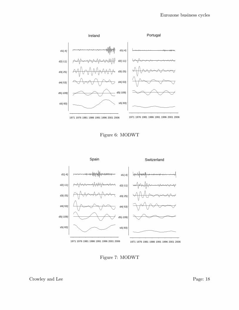
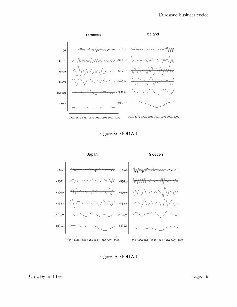
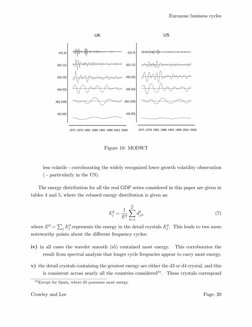
amounts as the scale order increases. Figure 2 shows MODWTs for the eurozone using an
s8 wavelet (a symmetric 8-tap �lter), and �gures 3 to 10 replicate the analysis for the other
countries in the dataset.
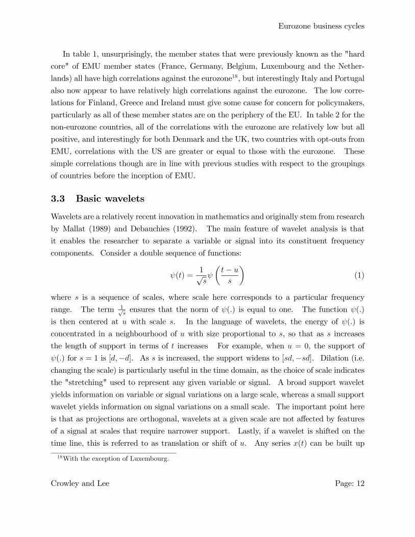
Several things are immediately apparent from stackplots:
i) apart from d1 crystal, which appears to contain mostly noise, there appear to be severalgrowth cycles of varying strength apparent in the data from the 2-4 quarter crystal
to lower frequencies, all with fairly regular cycles;
ii) although the wavelet smooth (s5) appears to dip during recessions, a coincidence ofdownward turns in growth cycles at di¤erent frequencies coincides with recessions;.
iii) up until the early 1980s in the case of the EU, and the mid-1980s in the case of the US,lower-order scale crystals (higher frequencies) d1 to d3 appear to contain higher energy
(stronger) cycles, whereas in the 1990s these lower-order scale cystals appeared to be
23The MODWT was found superior to both the cosine packet transform and the short-time Fouriertransform.
Crowley and Lee Page: 15
Eurozone business cycles
1971 1976 1981 1986 1991 1996 2001 2006
s5{93}
d5{109}
d4{53}
d3{25}
d2{11}
d1{4}
Eurozone
Year
Figure 2: MODWT
1971 1976 1981 1986 1991 1996 2001 2006
s5{93}
d5{109}
d4{53}
d3{25}
d2{11}
d1{4}
Germany
1971 1976 1981 1986 1991 1996 2001 2006
s5{93}
d5{109}
d4{53}
d3{25}
d2{11}
d1{4}
France
Figure 3: MODWT
Crowley and Lee Page: 16
Eurozone business cycles
1971 1976 1981 1986 1991 1996 2001 2006
s5{93}
d5{109}
d4{53}
d3{25}
d2{11}
d1{4}
Belgium
1971 1976 1981 1986 1991 1996 2001 2006
s5{93}
d5{109}
d4{53}
d3{25}
d2{11}
d1{4}
Italy
Figure 4: MODWT
1971 1976 1981 1986 1991 1996 2001 2006
s5{93}
d5{109}
d4{53}
d3{25}
d2{11}
d1{4}
Netherlands
1971 1976 1981 1986 1991 1996 2001 2006
s5{93}
d5{109}
d4{53}
d3{25}
d2{11}
d1{4}
Luxembourg
Figure 5: MODWT
Crowley and Lee Page: 17
Eurozone business cycles
1971 1976 1981 1986 1991 1996 2001 2006
s5{93}
d5{109}
d4{53}
d3{25}
d2{11}
d1{4}
Portugal
1971 1976 1981 1986 1991 1996 2001 2006
s5{93}
d5{109}
d4{53}
d3{25}
d2{11}
d1{4}
Ireland
Figure 6: MODWT
1971 1976 1981 1986 1991 1996 2001 2006
s5{93}
d5{109}
d4{53}
d3{25}
d2{11}
d1{4}
Spain
1971 1976 1981 1986 1991 1996 2001 2006
s5{93}
d5{109}
d4{53}
d3{25}
d2{11}
d1{4}
Switzerland
Figure 7: MODWT
Crowley and Lee Page: 18
Eurozone business cycles
1971 1976 1981 1986 1991 1996 2001 2006
s5{93}
d5{109}
d4{53}
d3{25}
d2{11}
d1{4}
Denmark
1971 1976 1981 1986 1991 1996 2001 2006
s5{93}
d5{109}
d4{53}
d3{25}
d2{11}
d1{4}
Iceland
Figure 8: MODWT
1971 1976 1981 1986 1991 1996 2001 2006
s5{93}
d5{109}
d4{53}
d3{25}
d2{11}
d1{4}
Japan
1971 1976 1981 1986 1991 1996 2001 2006
s5{93}
d5{109}
d4{53}
d3{25}
d2{11}
d1{4}
Sweden
Figure 9: MODWT
Crowley and Lee Page: 19
Eurozone business cycles
1971 1976 1981 1986 1991 1996 2001 2006
s5{93}
d5{109}
d4{53}
d3{25}
d2{11}
d1{4}
UK
1971 1976 1981 1986 1991 1996 2001 2006
s5{93}
d5{109}
d4{53}
d3{25}
d2{11}
d1{4}
US
Figure 10: MODWT
less volatile - corroborating the widely recognized lower growth volatility observation
( - particularly in the US).
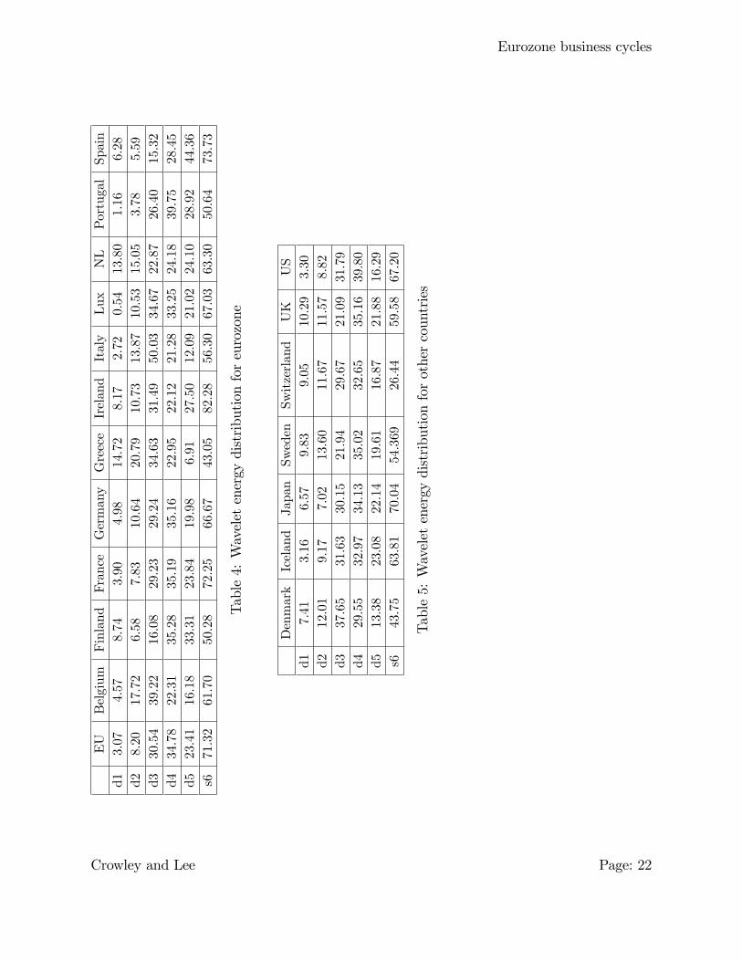
The energy distribution for all the real GDP series considered in this paper are given in
tables 4 and 5, where the rebased energy distribution is given as:
Edj =1
Ed
n
2jXk=1
d2j;k (7)
where Ed =P
j Edj :represents the energy in the detail crystals E
dj : This leads to two more
noteworthy points about the di¤erent frequency cycles:
iv) in all cases the wavelet smooth (s5) contained most energy. This corroborates the
result from spectral analysis that longer cycle freqencies appear to carry most energy.
v) the detail crystals containing the greatest energy are either the d3 or d4 crystal, and thisis consistent across nearly all the countries considered24. These crystals correspond
24Except for Spain, where d5 possesses most energy.
Crowley and Lee Page: 20
Eurozone business cycles
to cycles of 1-2 and 2-4 years, respectively, which tend to be at a slightly shorter
frequency than that of the conventional business cycle.
In tables 4 and 5, one of the issues is how to characterise the wavelet smooth in economic
terms. In theory, the wavelet smooth could incorporate longer term "trend" cycles, but
it could also just include residual "drift" in the growth rate of GDP. Clearly for the US
and the EU, the energy contained in the wavelet smooth is signi�cant, but for Switzerland,
an apparent outlier in this regard, the amount of energy contained in this crystal is not as
large, so suggesting that long cycles are not an empirical "stylized fact". Unfortunately,
though, in this study it is not possible to discern the nature of the content of this crystal,
given the length of the GDP series used.
Crowley and Lee Page: 21
Eurozone business cycles
EU
Belgium
Finland
France
Germany
Greece
Ireland
Italy
Lux
NL
PortugalSpain
d13.07
4.57
8.74
3.90
4.98
14.72
8.17
2.72
0.54
13.80
1.16
6.28
d28.20
17.72
6.58
7.83
10.64
20.79
10.73
13.87
10.53
15.05
3.78
5.59
d330.54
39.22
16.08
29.23
29.24
34.63
31.49
50.03
34.67
22.87
26.40
15.32
d434.78
22.31
35.28
35.19
35.16
22.95
22.12
21.28
33.25
24.18
39.75
28.45
d523.41
16.18
33.31
23.84
19.98
6.91
27.50
12.09
21.02
24.10
28.92
44.36
s671.32
61.70
50.28
72.25
66.67
43.05
82.28
56.30
67.03
63.30
50.64
73.73
Table4:Waveletenergydistributionforeurozone
Denmark
Iceland
Japan
Sweden
Switzerland
UK
US
d17.41
3.16
6.57
9.83
9.05
10.29
3.30
d212.01
9.17
7.02
13.60
11.67
11.57
8.82
d337.65
31.63
30.15
21.94
29.67
21.09
31.79
d429.55
32.97
34.13
35.02
32.65
35.16
39.80
d513.38
23.08
22.14
19.61
16.87
21.88
16.29
s643.75
63.81
70.04
54.369
26.44
59.58
67.20
Table5:Waveletenergydistributionforothercountries
Crowley and Lee Page: 22
Eurozone business cycles
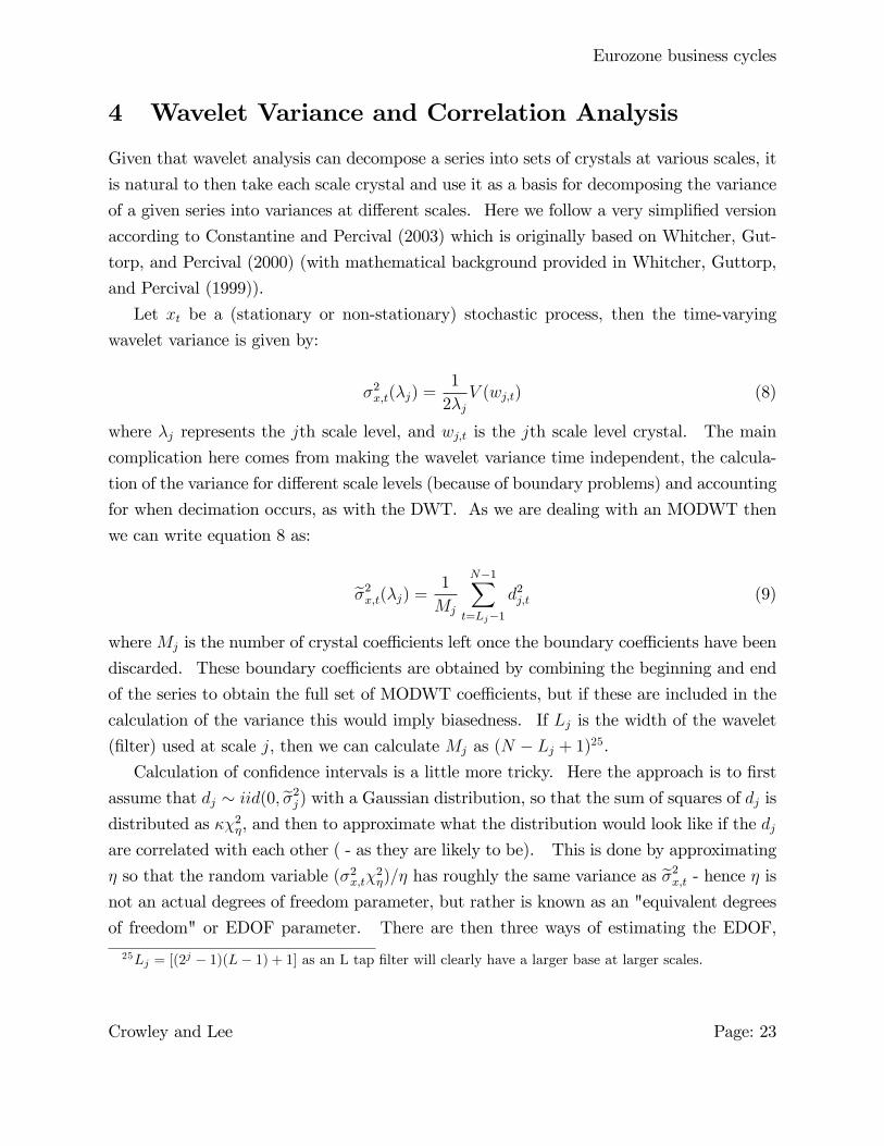
4 Wavelet Variance and Correlation Analysis
Given that wavelet analysis can decompose a series into sets of crystals at various scales, it
is natural to then take each scale crystal and use it as a basis for decomposing the variance
of a given series into variances at di¤erent scales. Here we follow a very simpli�ed version
according to Constantine and Percival (2003) which is originally based on Whitcher, Gut-
torp, and Percival (2000) (with mathematical background provided in Whitcher, Guttorp,
and Percival (1999)).
Let xt be a (stationary or non-stationary) stochastic process, then the time-varying
wavelet variance is given by:
�2x;t(�j) =1
2�jV (wj;t) (8)
where �j represents the jth scale level, and wj;t is the jth scale level crystal. The main
complication here comes from making the wavelet variance time independent, the calcula-
tion of the variance for di¤erent scale levels (because of boundary problems) and accounting
for when decimation occurs, as with the DWT. As we are dealing with an MODWT then
we can write equation 8 as:
e�2x;t(�j) = 1
Mj
N�1Xt=Lj�1
d2j;t (9)
whereMj is the number of crystal coe¢ cients left once the boundary coe¢ cients have been
discarded. These boundary coe¢ cients are obtained by combining the beginning and end
of the series to obtain the full set of MODWT coe¢ cients, but if these are included in the
calculation of the variance this would imply biasedness. If Lj is the width of the wavelet
(�lter) used at scale j, then we can calculate Mj as (N � Lj + 1)25.
Calculation of con�dence intervals is a little more tricky. Here the approach is to �rst
assume that dj � iid(0; e�2j) with a Gaussian distribution, so that the sum of squares of dj isdistributed as ��2�, and then to approximate what the distribution would look like if the djare correlated with each other ( - as they are likely to be). This is done by approximating
� so that the random variable (�2x;t�2�)=� has roughly the same variance as e�2x;t - hence � is
not an actual degrees of freedom parameter, but rather is known as an "equivalent degrees
of freedom" or EDOF parameter. There are then three ways of estimating the EDOF,
25Lj = [(2j � 1)(L� 1) + 1] as an L tap �lter will clearly have a larger base at larger scales.
Crowley and Lee Page: 23
Eurozone business cycles
based on i) large sample theory, ii) a priori knowledge of the spectral density function and
iii) a band-pass approximation. Here large sample theory is used to estimate the EDOF.
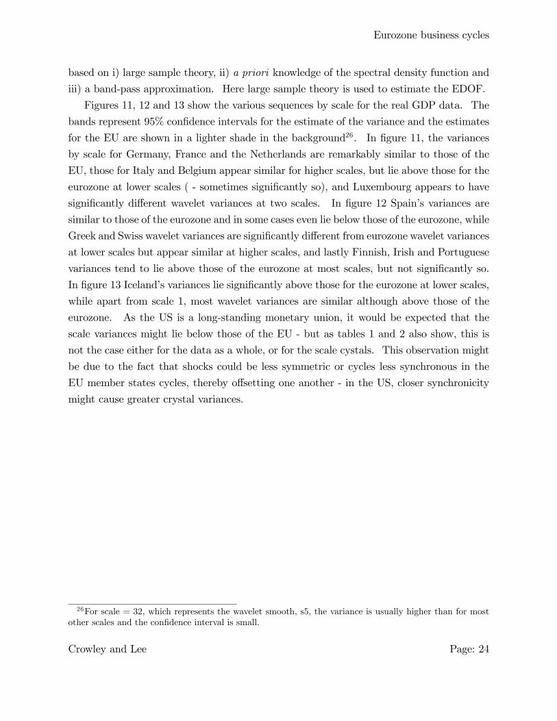
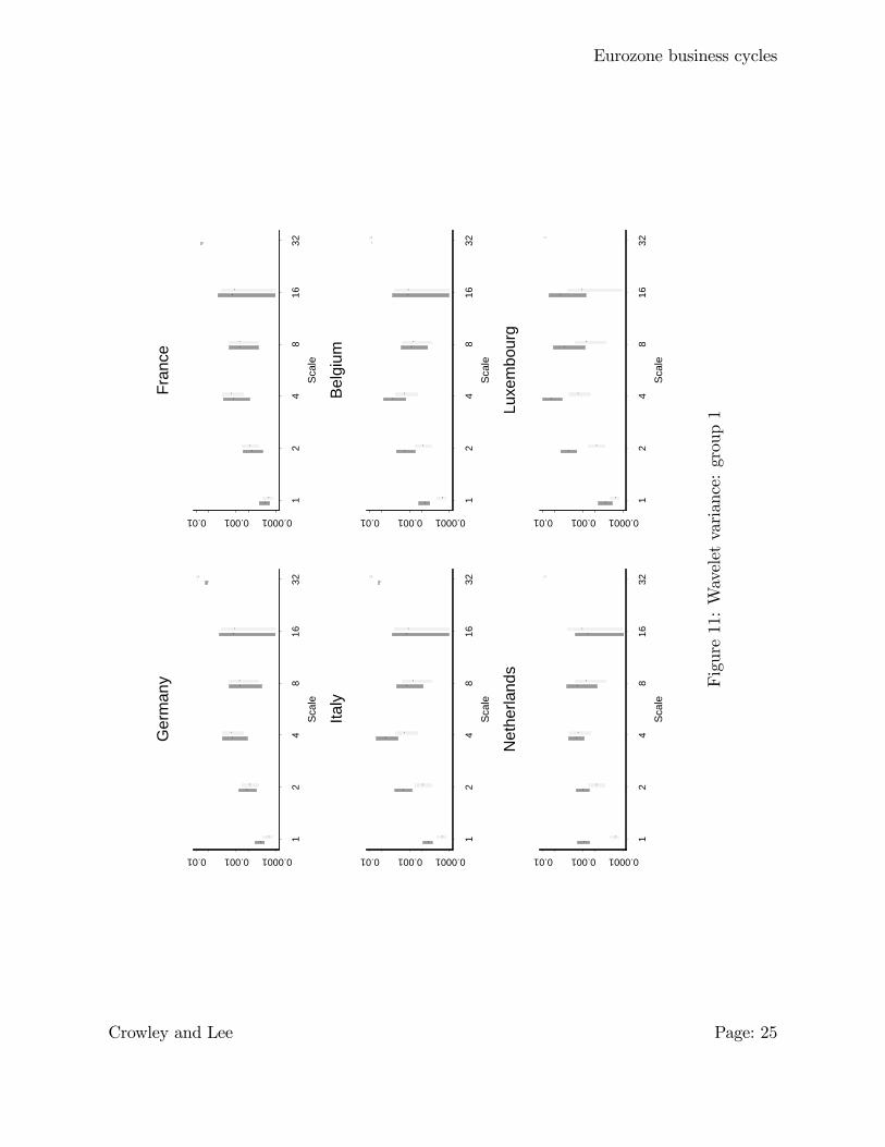
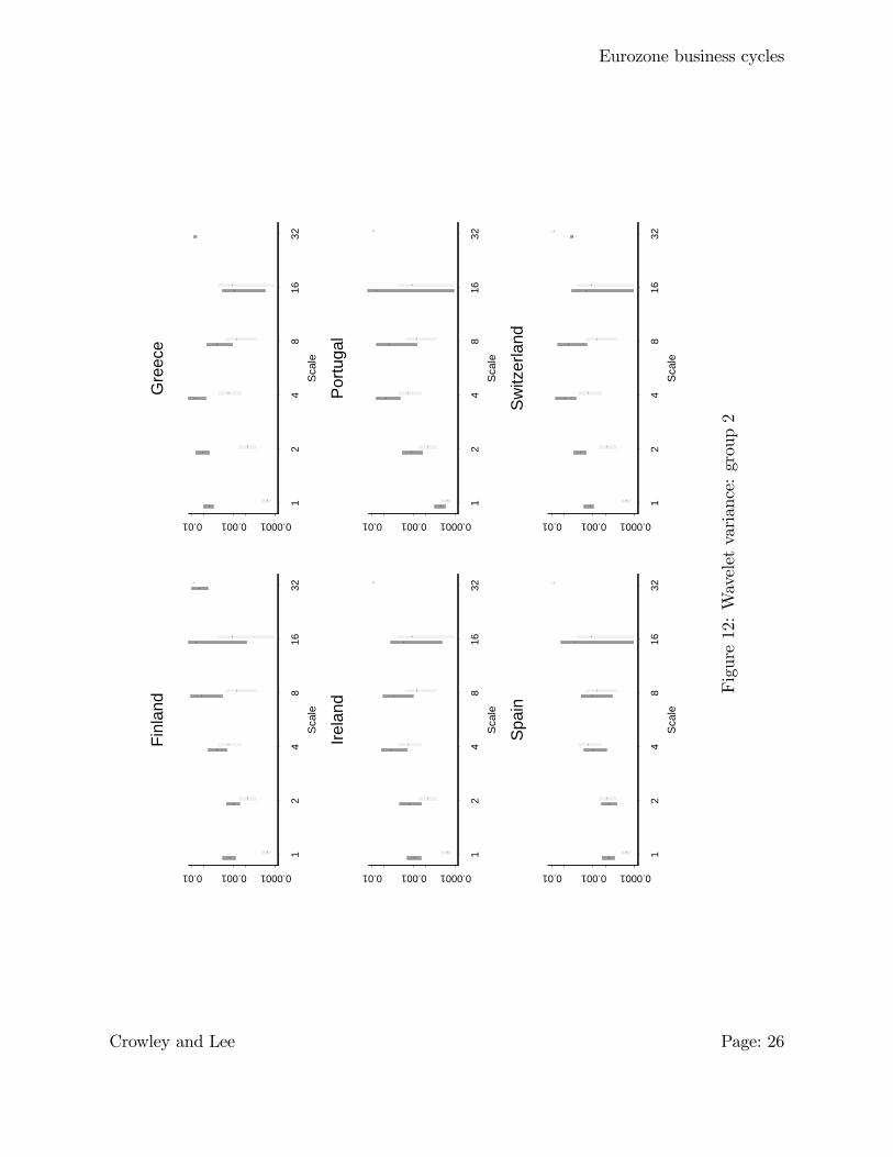
Figures 11, 12 and 13 show the various sequences by scale for the real GDP data. The
bands represent 95% con�dence intervals for the estimate of the variance and the estimates
for the EU are shown in a lighter shade in the background26. In �gure 11, the variances
by scale for Germany, France and the Netherlands are remarkably similar to those of the
EU, those for Italy and Belgium appear similar for higher scales, but lie above those for the
eurozone at lower scales ( - sometimes signi�cantly so), and Luxembourg appears to have
signi�cantly di¤erent wavelet variances at two scales. In �gure 12 Spain�s variances are
similar to those of the eurozone and in some cases even lie below those of the eurozone, while
Greek and Swiss wavelet variances are signi�cantly di¤erent from eurozone wavelet variances
at lower scales but appear similar at higher scales, and lastly Finnish, Irish and Portuguese
variances tend to lie above those of the eurozone at most scales, but not signi�cantly so.
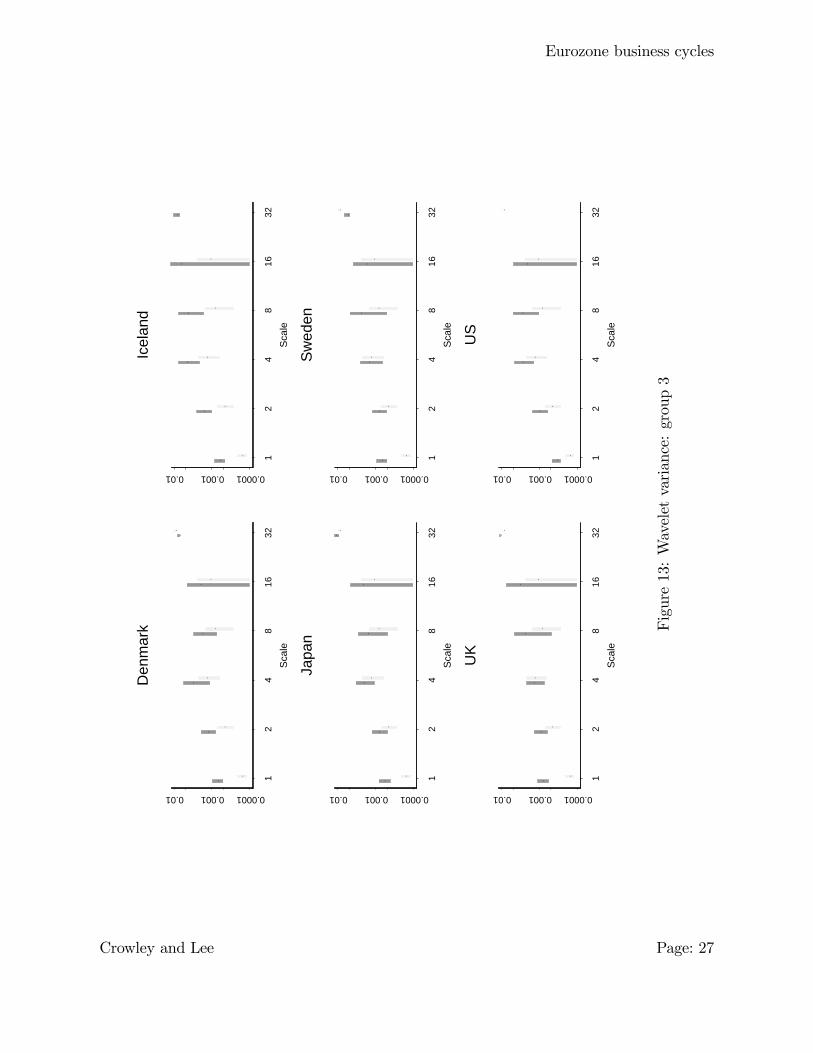
In �gure 13 Iceland�s variances lie signi�cantly above those for the eurozone at lower scales,
while apart from scale 1, most wavelet variances are similar although above those of the
eurozone. As the US is a long-standing monetary union, it would be expected that the
scale variances might lie below those of the EU - but as tables 1 and 2 also show, this is
not the case either for the data as a whole, or for the scale cystals. This observation might
be due to the fact that shocks could be less symmetric or cycles less synchronous in the
EU member states cycles, thereby o¤setting one another - in the US, closer synchronicity
might cause greater crystal variances.
26For scale = 32, which represents the wavelet smooth, s5, the variance is usually higher than for mostother scales and the con�dence interval is small.
Crowley and Lee Page: 24
Eurozone business cycles
12
48
1632
Sca
le
0.00010.0010.01
Ger
man
y
12
48
1632
Sca
le
0.00010.0010.01
Fran
ce
12
48
1632
Sca
le
0.00010.0010.01
Italy
12
48
1632
Sca
le
0.00010.0010.01
Belg
ium
12
48
1632
Sca
le
0.00010.0010.01
Net
herla
nds
12
48
1632
Sca
le
0.00010.0010.01
Luxe
mbo
urg
Figure11:Waveletvariance:group1
Crowley and Lee Page: 25
Eurozone business cycles
12
48
1632
Sca
le
0.00010.0010.01
Finl
and
12
48
1632
Sca
le
0.00010.0010.01
Gre
ece
12
48
1632
Sca
le
0.00010.0010.01
Irela
nd
12
48
1632
Sca
le
0.00010.0010.01
Portu
gal
12
48
1632
Sca
le
0.00010.0010.01
Spai
n
12
48
1632
Sca
le
0.00010.0010.01
Switz
erla
nd
Figure12:Waveletvariance:group2
Crowley and Lee Page: 26
Eurozone business cycles
12
48
1632
Sca
le
0.00010.0010.01
Den
mar
k
12
48
1632
Sca
le
0.00010.0010.01
Icel
and
12
48
1632
Sca
le
0.00010.0010.01
Japa
n
12
48
1632
Sca
le
0.00010.0010.01
Swed
en
12
48
1632
Sca
le
0.00010.0010.01
UK
12
48
1632
Sca
le
0.00010.0010.01
US
Figure13:Waveletvariance:group3
Crowley and Lee Page: 27
Eurozone business cycles
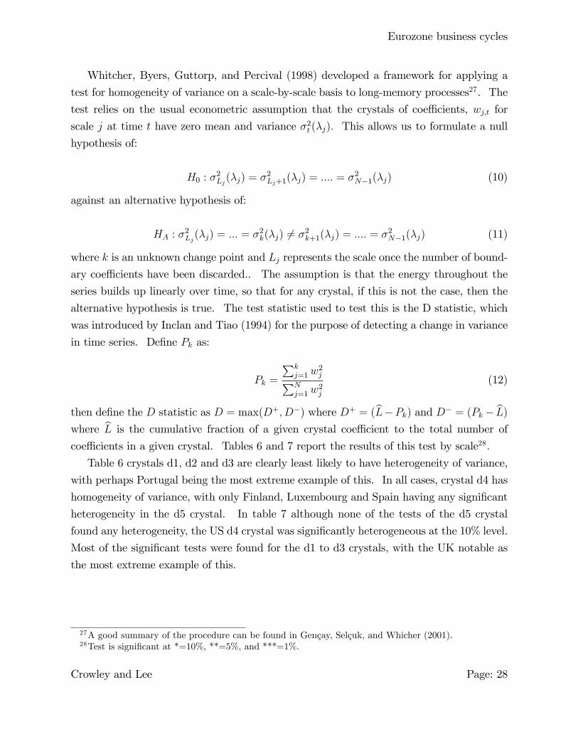
Whitcher, Byers, Guttorp, and Percival (1998) developed a framework for applying a
test for homogeneity of variance on a scale-by-scale basis to long-memory processes27. The
test relies on the usual econometric assumption that the crystals of coe¢ cients, wj;t for
scale j at time t have zero mean and variance �2t (�j): This allows us to formulate a null
hypothesis of:
H0 : �2Lj(�j) = �2Lj+1(�j) = :::: = �2N�1(�j) (10)
against an alternative hypothesis of:
HA : �2Lj(�j) = ::: = �2k(�j) 6= �2k+1(�j) = :::: = �2N�1(�j) (11)
where k is an unknown change point and Lj represents the scale once the number of bound-
ary coe¢ cients have been discarded.. The assumption is that the energy throughout the
series builds up linearly over time, so that for any crystal, if this is not the case, then the
alternative hypothesis is true. The test statistic used to test this is the D statistic, which
was introduced by Inclan and Tiao (1994) for the purpose of detecting a change in variance
in time series. De�ne Pk as:
Pk =
Pkj=1w
2jPN
j=1w2j
(12)
then de�ne the D statistic as D = max(D+; D�) where D+ = (bL�Pk) and D� = (Pk� bL)where bL is the cumulative fraction of a given crystal coe¢ cient to the total number of
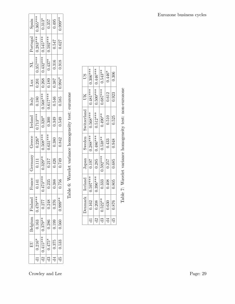
coe¢ cients in a given crystal. Tables 6 and 7 report the results of this test by scale28.
Table 6 crystals d1, d2 and d3 are clearly least likely to have heterogeneity of variance,
with perhaps Portugal being the most extreme example of this. In all cases, crystal d4 has
homogeneity of variance, with only Finland, Luxembourg and Spain having any signi�cant
heterogeneity in the d5 crystal. In table 7 although none of the tests of the d5 crystal
found any heterogeneity, the US d4 crystal was signi�cantly heterogeneous at the 10% level.
Most of the signi�cant tests were found for the d1 to d3 crystals, with the UK notable as
the most extreme example of this.
27A good summary of the procedure can be found in Gençay, Selçuk, and Whicher (2001).28Test is signi�cant at *=10%, **=5%, and ***=1%.
Crowley and Lee Page: 28
Eurozone business cycles
EU
Belgium
Finland
France
Germany
Greece
Ireland
Italy
Lux
NL
Portugal
Spain
d10.216*
0.163
0.479***
0.141
0.111
0.226*
0.713***
0.180
0.201
0.357***
0.283***
0.365***
d20.415***
0.379**
0.277
0.473***
0.329**
0.508***
0.320*
0.568***
0.268
0.432***
0.545***
0.313*
d30.475*
0.286
0.248
0.235
0.217
0.631***
0.300
0.617***
0.189
0.437*
0.592***
0.357
d40.375
0.199
0.376
0.388
0.426
0.380
0.349
0.546
0.387
0.316
0.547
0.495
d50.533
0.560
0.999**
0.756
0.749
0.842
0.549
0.585
0.994*
0.918
0.627
0.999**
Table6:Waveletvariancehomogeneitytest:eurozone
Denmark
Iceland
Japan
Sweden
Switzerland
UK
US
d10.162
0.597***
0.197
0.288***
0.568***
0.481***
0.306***
d20.208
0.396***
0.285
0.486***
0.512***
0.500***
0.446***
d30.522**
0.333
0.592***
0.538**
0.490**
0.687***
0.543**
d40.630
0.408
0.257
0.433
0.510
0.612
0.446*
d50.876
0.805
0.685
0.948
0.525
0.923
0.306
Table7:Waveletvariancehomogeneitytest:non-eurozone
Crowley and Lee Page: 29
Eurozone business cycles
Covariance by scale can also be obtained using similar methods to those described above,
so that wavelet variances and covariances can be used together to obtain scale correlations
between series and con�dence intervals can be derived for the correlation coe¢ cients by scale
(these are derived in Whitcher, Guttorp, and Percival (2000)). The correlation between
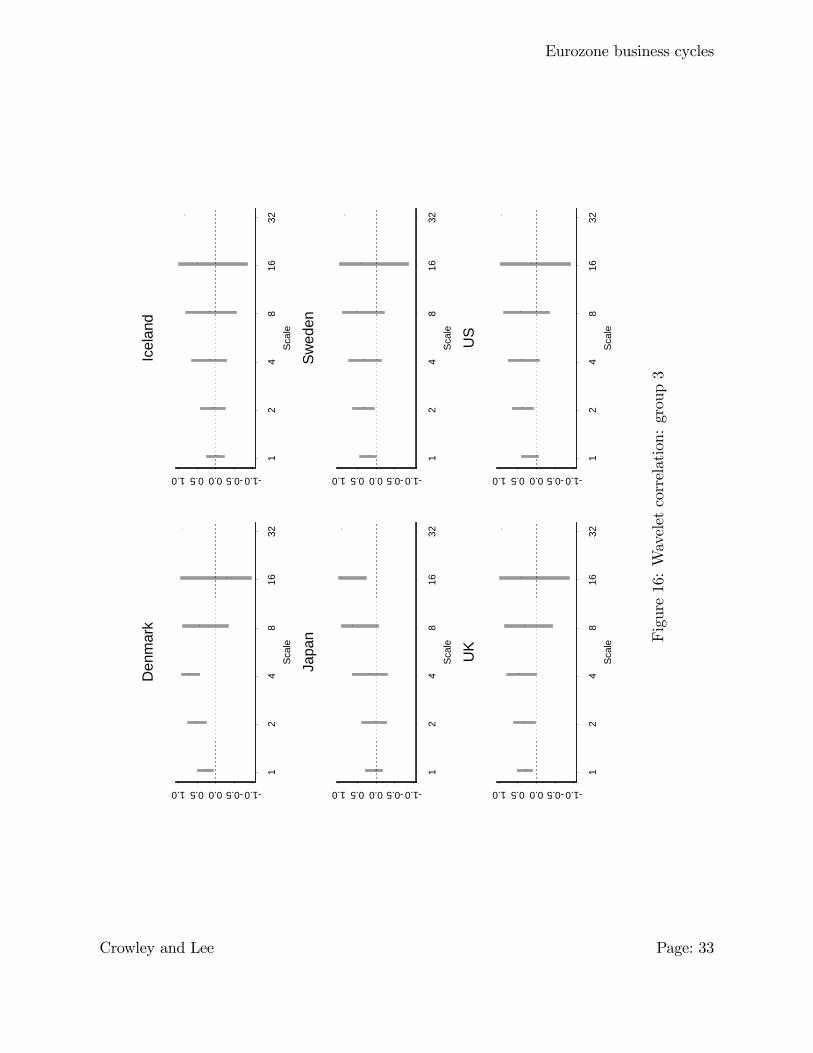
the various real GDP series and the eurozone are estimated and plotted in �gures 14, 15 and
16 by scale, although for the wavelet smooth, s5, denoted scale=32 only point estimates of
correlation are shown, as no correction can be made for boundary e¤ects given that there
is no de�ned frequency band for the wavelet smooth.
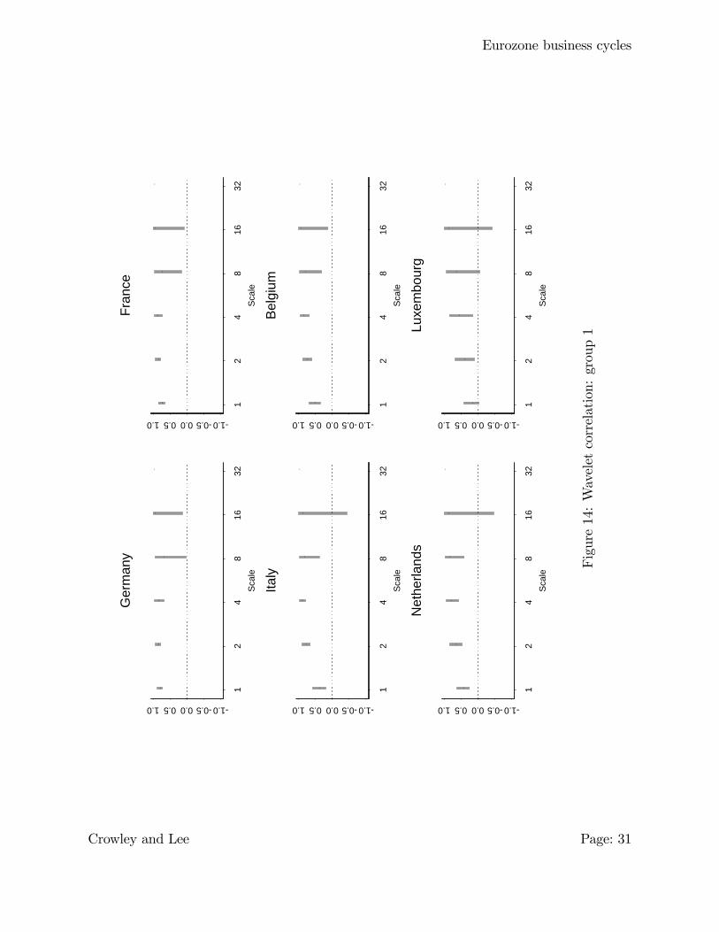
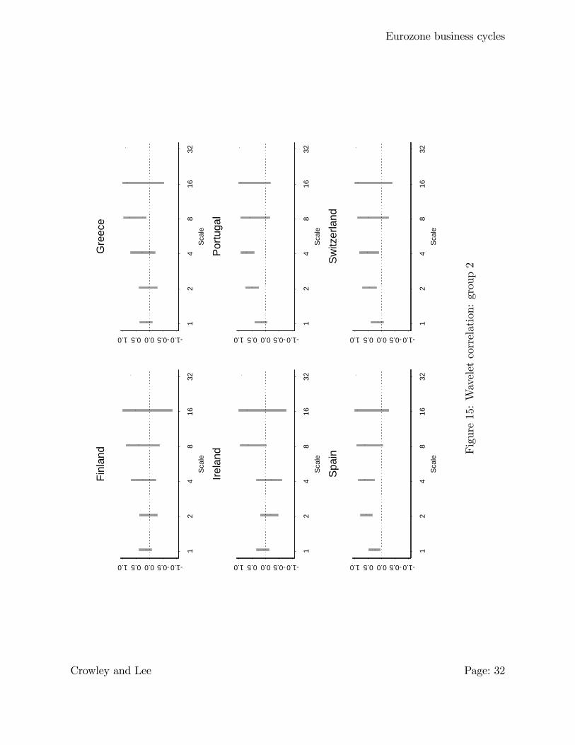
The di¤erence between �gure 14 and 15 is certainly quite striking. In �gure 14, France
appears to possess the highest correlations by scale, with Germany closely following, but
Luxembourg possesses low correlations for the d1 crystal, and for d4 and d5 correlations,
these are not signi�cantly di¤erent from zero. In �gure 15, Finland and Ireland have no
wavelet correlations that are signi�cantly di¤erent from zero, and for Portugal, Spain and
Switzerland, only the d2 and d3 crystal correlations are signi�cantly di¤erent from zero. In
�gure 16 only Denmark possesses 3 sets of crystals with signi�cantly positive correlations,
while Japan, Sweden, the UK and US only have one signi�cantly crystal correlation, while
Iceland possesses none.
This analysis of correlation at di¤erent growth cycle periodicities demonstrates that
although there is a high degree of correlation in longer cycles, for shorter cycles, these
correlations are not always signi�cantly di¤erent from zero. The sample of EU member
states roughly divides into 4 groups:
a) those member states that have signi�cantly positive correlations at all cycle frequencies(Germany, France and Belgium);
b) those member states that have signi�cantly positive correlations except for the d5 crys-tal, representing 4-8 year cycles (Italy, Netherlands);
c) those member states that have two or more signi�cantly positive crystal correlations(Luxembourg, Portugal, Spain, Switzerland and Denmark); and
d) those member states that have one or less sign�cantly positive crystal correlations (Fin-land, Greece, Ireland, Sweden, UK)
Crowley and Lee Page: 30
Eurozone business cycles
12
48
1632
Sca
le
1.00.50.00.51.0
Ger
man
y
12
48
1632
Sca
le
1.00.50.00.51.0
Fran
ce
12
48
1632
Sca
le
1.00.50.00.51.0
Italy
12
48
1632
Sca
le
1.00.50.00.51.0
Belg
ium
12
48
1632
Sca
le
1.00.50.00.51.0
Net
herla
nds
12
48
1632
Sca
le
1.00.50.00.51.0
Luxe
mbo
urg
Figure14:Waveletcorrelation:group1
Crowley and Lee Page: 31
Eurozone business cycles
12
48
1632
Sca
le
1.00.50.00.51.0
Finl
and
12
48
1632
Sca
le
1.00.50.00.51.0
Gre
ece
12
48
1632
Sca
le
1.00.50.00.51.0
Irela
nd
12
48
1632
Sca
le
1.00.50.00.51.0
Por
tuga
l
12
48
1632
Sca
le
1.00.50.00.51.0
Spai
n
12
48
1632
Sca
le
1.00.50.00.51.0
Sw
itzer
land
Figure15:Waveletcorrelation:group2
Crowley and Lee Page: 32
Eurozone business cycles
12
48
1632
Scal
e
1.00.50.00.51.0
Den
mar
k
12
48
1632
Scal
e
1.00.50.00.51.0
Icel
and
12
48
1632
Scal
e
1.00.50.00.51.0
Japa
n
12
48
1632
Scal
e
1.00.50.00.51.0
Swed
en
12
48
1632
Scal
e
1.00.50.00.51.0
UK
12
48
1632
Scal
e
1.00.50.00.51.0
US
Figure16:Waveletcorrelation:group3
Crowley and Lee Page: 33
Eurozone business cycles
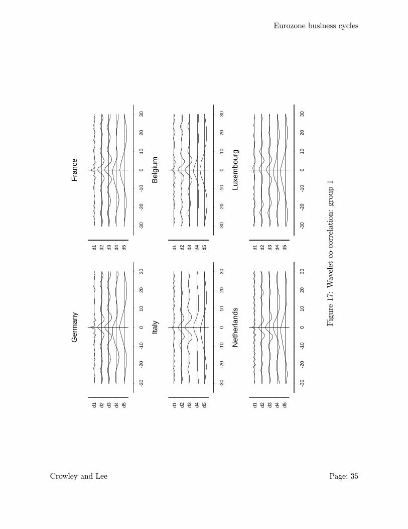
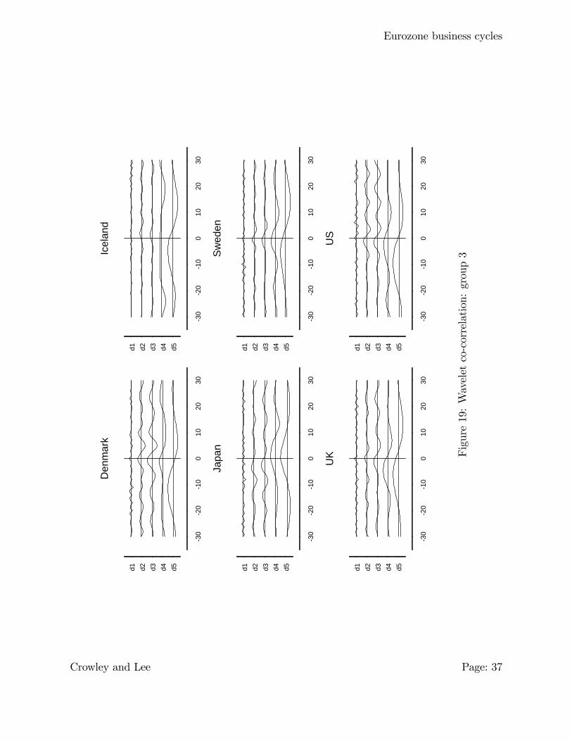
Once scale correlations have been obtained, co-correlations can be calculated so as to
study the phase relationship versus the eurozone. Each crystal is lagged against its euro-
zone equivalent and �gures 17, 18 and 19 show co-correlations29 . These co-correlations
measure only how the correlations change by lagging the country series against the equiva-
lent eurozone series, so they are able to study phasing of cycles rather than the magnitude
of the correlations themselves. The co-correlations against the eurozone in �gure 17 indi-
cate that all these eurozone countries have particularly synchronous growth cycles to those
of the EU, with no phasing issue at any cycle except perhaps for the d4 crystal in the case
of Germany and France (where there is a slight lead) and the d5 crystal in the case of Italy
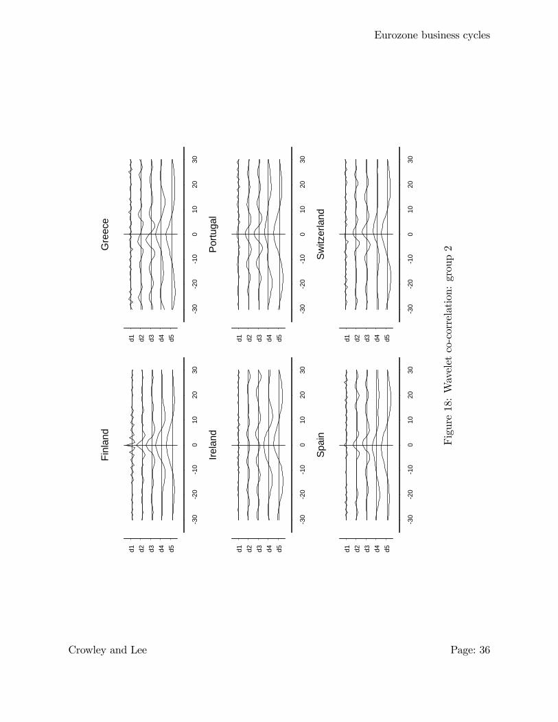
and the Netherlands (again, a lead). In �gure 18, Finland, Portugal and Spain tend to
have relatively synchronous cycles with the eurozone, but Greece and Ireland only have
synchronicity in the higher order crystals, with Ireland having negative contemporaneous
correlations for d2 and d3 crystals, as could be seen also in �gure 15. Switzerland also
appears not to be have zero phase against the eurozone, but here it appears that there is a
lag relationship of roughly 2 quarters in the d3 and d4 crystals. Turning to �gure 19, what
is striking here is the similarity between the co-correlation plots for the UK, Sweden and
the US. In all cases there is a lead relationship with the eurozone, particularly at longer
cycles, with the d5 crystal indicating roughly a 10 quarter lead against the eurozone for
the US, and roughly an 8 quarter lead for the UK. Denmark is synchronous in shorter
cycles, but verging on being asynchronous in its d5 crystal. Iceland appears not to have
any high correlations against the eurozone at shorter frequencies, but has a lead against
the eurozone in its d5 crystal, and Japan is only synchronous in longer term cycles.
In terms of synchronicity of cycles, then, the eurozone members roughly fall into the
following groupings:
a) those member states that are relatively well synchronised against the eurozone (Ger-many, France, Italy, Belgium, Netherlands, Luxembourg, Finland, Portugal and Spain);
b) those member states that are synchronised at high frequency cycles, but not at lowfrequency cycles (Denmark, Sweden and the UK); and
c) those member states that are synchronised at low frequency cycles, but not at high
frequency cycles (Greece and Ireland).
29The x-axis refers to the lag of the country detail crystal against the eurozone equivalent. Hence ahigh correlation at -5 indicates the correlation value if the country series is lagged by 5 quarters againstthe eurozone aggregate.
Crowley and Lee Page: 34
Eurozone business cycles
30
20
10
010
2030
d5d4d3d2d1
Ger
man
y
30
20
10
010
2030
d5d4d3d2d1
Fran
ce
30
20
10
010
2030
d5d4d3d2d1
Italy
30
20
10
010
2030
d5d4d3d2d1
Belg
ium
30
20
10
010
2030
d5d4d3d2d1
Net
herla
nds
30
20
10
010
2030
d5d4d3d2d1
Luxe
mbo
urg
Figure17:Waveletco-correlation:group1
Crowley and Lee Page: 35
Eurozone business cycles
30
20
10
010
2030
d5d4d3d2d1
Finl
and
30
20
10
010
2030
d5d4d3d2d1
Gre
ece
30
20
10
010
2030
d5d4d3d2d1
Irela
nd
30
20
10
010
2030
d5d4d3d2d1
Portu
gal
30
20
10
010
2030
d5d4d3d2d1
Spai
n
30
20
10
010
2030
d5d4d3d2d1
Switz
erla
nd
Figure18:Waveletco-correlation:group2
Crowley and Lee Page: 36
Eurozone business cycles
30
20
10
010
2030
d5d4d3d2d1
Den
mar
k
30
20
10
010
2030
d5d4d3d2d1
Icel
and
30
20
10
010
2030
d5d4d3d2d1
Japa
n
30
20
10
010
2030
d5d4d3d2d1
Swed
en
30
20
10
010
2030
d5d4d3d2d1
UK
30
20
10
010
2030
d5d4d3d2d1
US
Figure19:Waveletco-correlation:group3
Crowley and Lee Page: 37
Eurozone business cycles
5 Dynamic conditional correlation (DCC) analysis
5.1 Methodology
The analysis so far has been of a static nature, but it is useful to have some idea of
how these wavlet correlations change through time. In order to do this, Engle�s DCC
analysis is used30. Although the notion of dynamic correlation has traditionally been
implemented by use of rolling regressions, Engle (2002) introduced the notion of DCC using
the GARCH framework of time series analysis, so as to incorporate conditional correlations
into a dynamic framework. Full details of this approach are available in Engle and Sheppard
(2001) - below only an abridged version of the approach is presented.
Let yjt =�y1jt y2jt
�0be a vector containing the two crystals from the real GDP series,
one for the country concerned and the other for the EU series. Dropping the j subscript
denoting the crystal scale for ease of exposition, then a conditional mean equation in reduced
form VAR format can be written as:
A(L)yt = "t (13)
where A(L) is a polynomial matrix in the lag operator, L, and "t � N(0;Ht);for all t,
where Ht is a conditional variance-covariance matrix. The DCC-GARCH framework can
be best understood by re-writing Ht as:
Ht = DtRtDt (14)
where Dt = diag�p
hitis a 2x2 diagonal matrix of time-varying standard deviations
from univariate GARCH models and Rt ���ijfor i; j = 1; 2; :where �ij are conditional
correlation coe¢ cients. The elements in Dt follow a univariate GARCH(p,q) process in
the following manner:
hit = !i +
PiXp=1
�ip"2it�p +
QiXq=1
�iqhit�q (15)
Engle (2002) had a speci�c structure for the DCC(M,N) process, and it can be reproduced
as:
Rt = Q��1t QtQ��1t (16)
30This was implemented using the RATS program.
Crowley and Lee Page: 38
Eurozone business cycles
where:
Qt = (1�MXm=1
am �NXn=1
bn)Q+
MXm=1
am(�t�m�0
t�m) +NXn=1
bnQt�n (17)
where �t = "it=phit; which is a vector containing standardized errors, Qt � fqijgt is the
conditional variance-covariance matrix of standardized errors with its unconditional vari-
ance covariance matrix, Q;obtained from the �rst stage of estimation, and Q�t is a diagonal
matrix containing the square root of the diagonal elements of Qt:
Q�t =
� pq11 00
pq22
�(18)
From Rt; the conditional correlation between y1t and y2t can be obtained, namely:
�12;t =q12;tpq11;tq22;t
(19)
The system is estimated using the maximum likelihood method in which the log-likelihood
can be expressed as:
L = �12
TXt=1
n2 log(2�) + 2 log jDtj+ log jRtj+ �
0
tR�1t �t
o(20)
The estimation approach is then as follows:
i) obtain one period ahead residuals from the estimation of a bivariate VAR of y1t on
y2t with lag length selected by the Bayesian information criterion;
ii) estimate the univariate GARCH processes for the output and price residuals; then
iii) estimate the conditional correlation matrix (Rt) using the log-likelihood function (eqn.
20) conditional on the GARCH parameter estimates in ii).
5.2 Empirical results
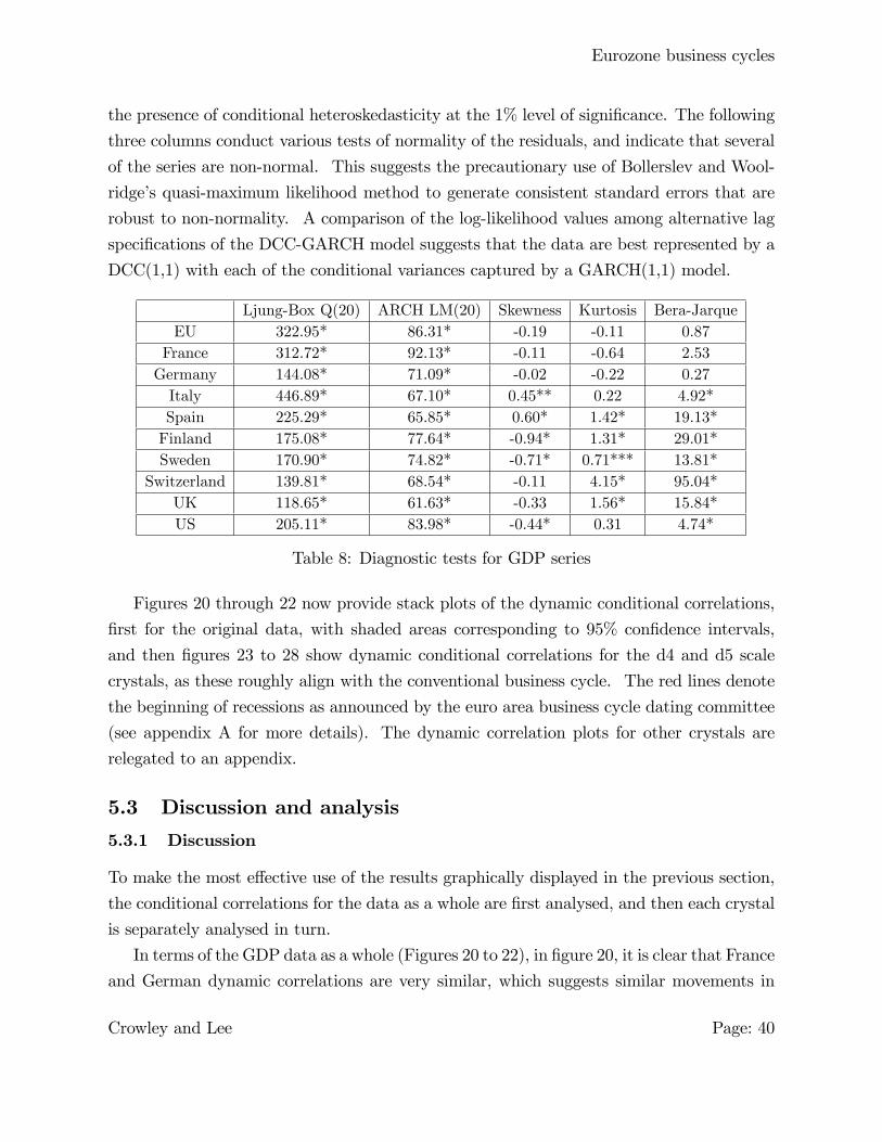
Table 7 provides some diagnostics for the series as a whole. The �rst panel of the table
reports the Ljung-Box test for serial correlation using the squares of the residuals. The
Q-statistics for an order of 20 clearly indicate the presence of serial correlations in both
the original series and the d4 crystal at the 1% level of signi�cance. The second column
of both tables shows test results for Engle�s LM test for ARCH with 20 lags, and indicates
Crowley and Lee Page: 39
Eurozone business cycles
the presence of conditional heteroskedasticity at the 1% level of signi�cance. The following
three columns conduct various tests of normality of the residuals, and indicate that several
of the series are non-normal. This suggests the precautionary use of Bollerslev and Wool-
ridge�s quasi-maximum likelihood method to generate consistent standard errors that are
robust to non-normality. A comparison of the log-likelihood values among alternative lag
speci�cations of the DCC-GARCH model suggests that the data are best represented by a
DCC(1,1) with each of the conditional variances captured by a GARCH(1,1) model.
Ljung-Box Q(20) ARCH LM(20) Skewness Kurtosis Bera-JarqueEU 322.95* 86.31* -0.19 -0.11 0.87France 312.72* 92.13* -0.11 -0.64 2.53Germany 144.08* 71.09* -0.02 -0.22 0.27Italy 446.89* 67.10* 0.45** 0.22 4.92*Spain 225.29* 65.85* 0.60* 1.42* 19.13*Finland 175.08* 77.64* -0.94* 1.31* 29.01*Sweden 170.90* 74.82* -0.71* 0.71*** 13.81*
Switzerland 139.81* 68.54* -0.11 4.15* 95.04*UK 118.65* 61.63* -0.33 1.56* 15.84*US 205.11* 83.98* -0.44* 0.31 4.74*
Table 8: Diagnostic tests for GDP series
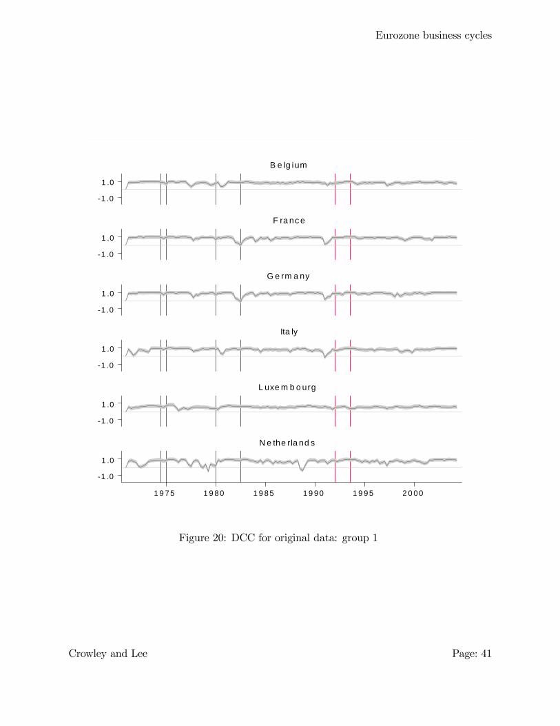
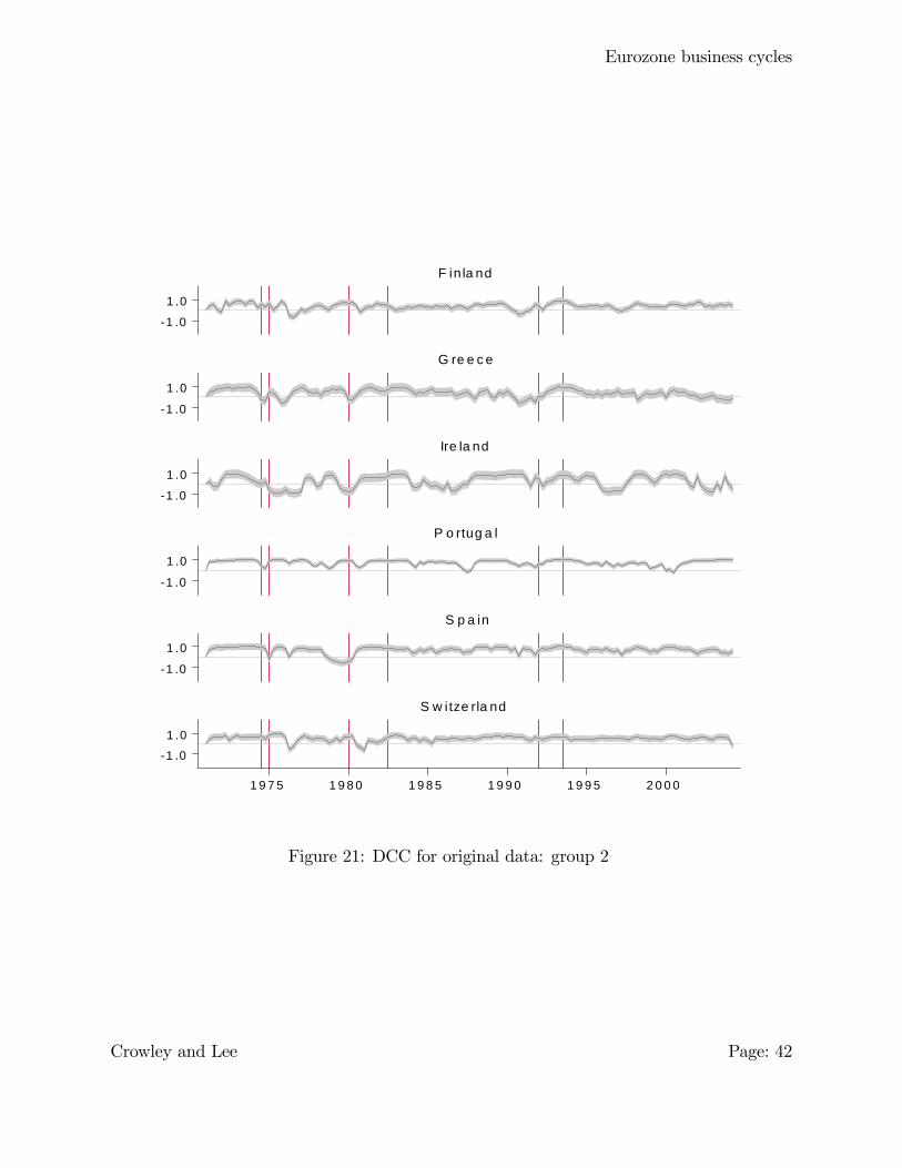
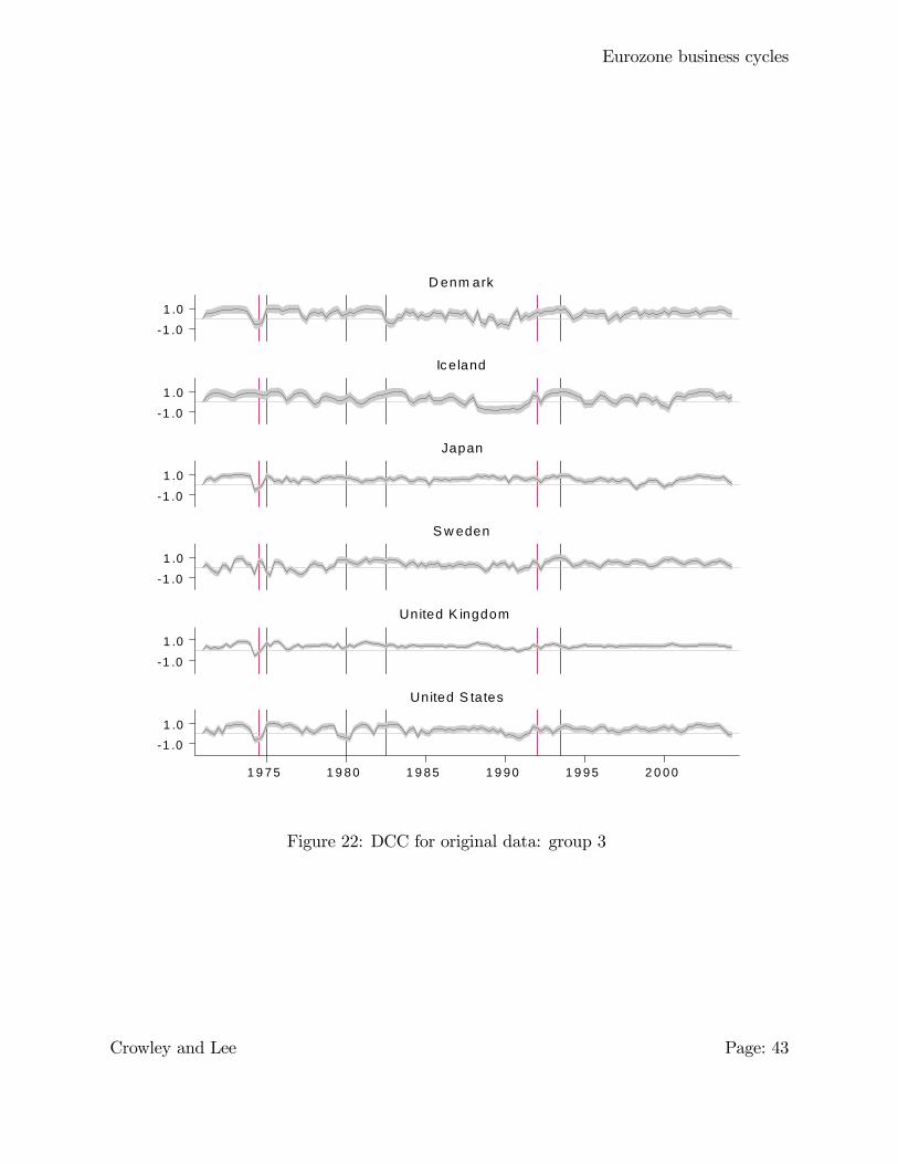
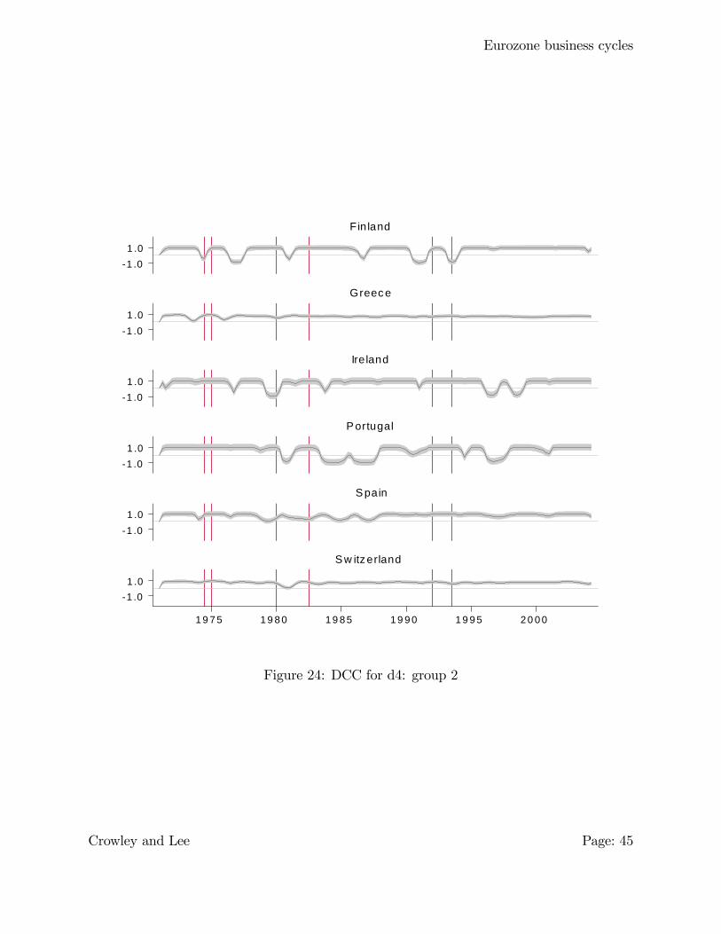
Figures 20 through 22 now provide stack plots of the dynamic conditional correlations,
�rst for the original data, with shaded areas corresponding to 95% con�dence intervals,
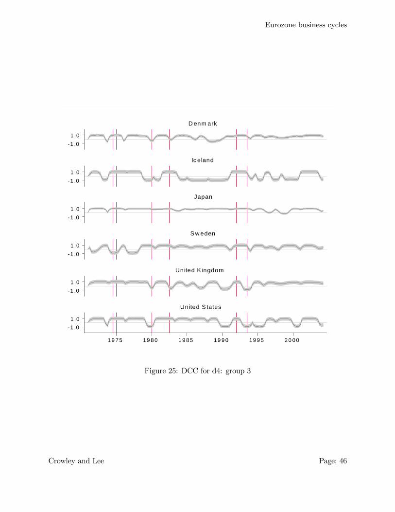
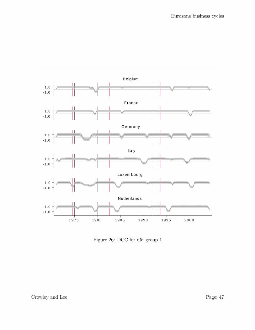
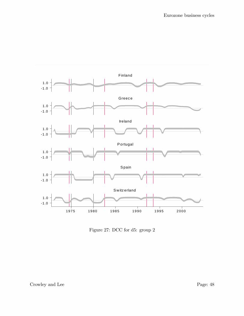
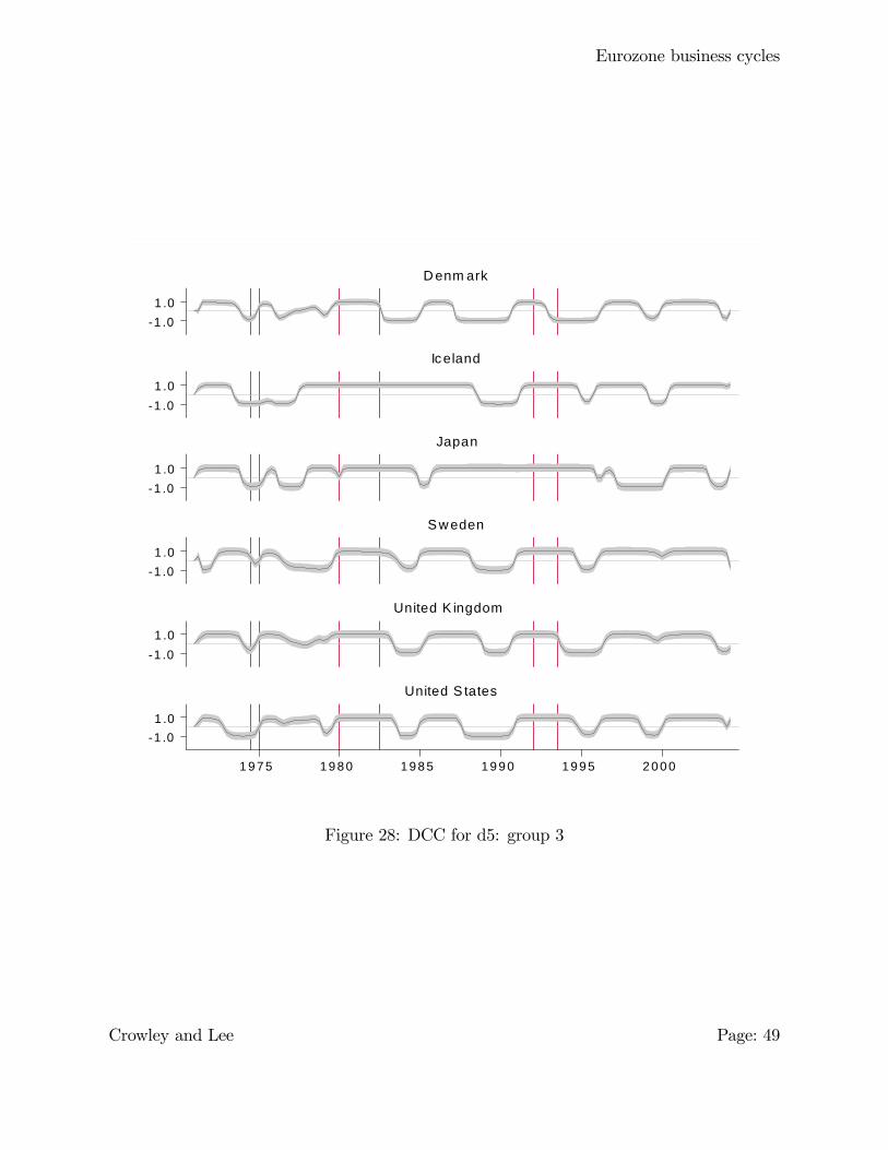
and then �gures 23 to 28 show dynamic conditional correlations for the d4 and d5 scale
crystals, as these roughly align with the conventional business cycle. The red lines denote
the beginning of recessions as announced by the euro area business cycle dating committee
(see appendix A for more details). The dynamic correlation plots for other crystals are
relegated to an appendix.
5.3 Discussion and analysis
5.3.1 Discussion
To make the most e¤ective use of the results graphically displayed in the previous section,
the conditional correlations for the data as a whole are �rst analysed, and then each crystal
is separately analysed in turn.
In terms of the GDP data as a whole (Figures 20 to 22), in �gure 20, it is clear that France
and German dynamic correlations are very similar, which suggests similar movements in
Crowley and Lee Page: 40
Eurozone business cycles
1 .0
1 .0
1 .0
1 .0
1 .0
1 .0
1 .0
1 .0
1 .0
1 .0
1 .0
1 .0
1 9 7 5 1 9 8 0 1 9 8 5 1 9 9 0 1 9 9 5 2 0 0 0
B e lg ium
F ra nc e
G e rm a ny
Ita ly
L uxe m b o urg
N e the rla nd s
Figure 20: DCC for original data: group 1
Crowley and Lee Page: 41
Eurozone business cycles
1 .0
1 .0
1 .0
1 .0
1 .0
1 .0
1 .0
1 .0
1 .0
1 .0
1 .0
1 .0
1 9 7 5 1 9 8 0 1 9 8 5 1 9 9 0 1 9 9 5 2 0 0 0
F inla nd
G re e c e
Ire la nd
P o rtug a l
S p a in
S w itze rla nd
Figure 21: DCC for original data: group 2
Crowley and Lee Page: 42
Eurozone business cycles
1 .0
1 .0
1 .0
1 .0
1 .0
1 .0
1 .0
1 .0
1 .0
1 .0
1 .01 .0
1 9 7 5 1 9 8 0 1 9 8 5 1 9 9 0 1 9 9 5 2 0 0 0
D enm ark
Ic eland
Japan
S w eden
United K ingdom
United S tates
Figure 22: DCC for original data: group 3
Crowley and Lee Page: 43

Eurozone business cycles
1 .01 .0
1 .01 .0
1 .01 .0
1 .01 .0
1 .01 .0
1 .01 .0
1 9 7 5 1 9 8 0 1 9 8 5 1 9 9 0 1 9 9 5 2 0 0 0
B elgium
Franc e
Germ any
Italy
Luxem bourg
Netherlands
Figure 23: DCC for d4: group 1
Crowley and Lee Page: 44
Eurozone business cycles
1 .01 .0
1 .01 .0
1 .01 .0
1 .01 .0
1 .01 .0
1 .01 .0
1 9 7 5 1 9 8 0 1 9 8 5 1 9 9 0 1 9 9 5 2 0 0 0
Finland
Greec e
Ire land
P ortugal
S pain
S w itzerland
Figure 24: DCC for d4: group 2
Crowley and Lee Page: 45
Eurozone business cycles
1 .01 .0
1 .01 .0
1 .01 .0
1 .01 .0
1 .01 .0
1 .01 .0
1 9 7 5 1 9 8 0 1 9 8 5 1 9 9 0 1 9 9 5 2 0 0 0
D enm ark
Ic eland
Japan
S w eden
United K ingdom
United S tates
Figure 25: DCC for d4: group 3
Crowley and Lee Page: 46
Eurozone business cycles
1 .01 .0
1 .01 .0
1 .01 .0
1 .01 .0
1 .01 .0
1 .01 .0
1 9 7 5 1 9 8 0 1 9 8 5 1 9 9 0 1 9 9 5 2 0 0 0
B elgium
Franc e
Germ any
Ita ly
Luxem bourg
Netherlands
Figure 26: DCC for d5: group 1
Crowley and Lee Page: 47
Eurozone business cycles
1 .01 .0
1 .01 .0
1 .01 .0
1 .01 .0
1 .01 .0
1 .01 .0
1 9 7 5 1 9 8 0 1 9 8 5 1 9 9 0 1 9 9 5 2 0 0 0
Finland
Greec e
Ireland
P ortugal
S pain
S w itz erland
Figure 27: DCC for d5: group 2
Crowley and Lee Page: 48
Eurozone business cycles
1 .01 .0
1 .01 .0
1 .01 .0
1 .01 .0
1 .01 .0
1 .01 .0
1 9 7 5 1 9 8 0 1 9 8 5 1 9 9 0 1 9 9 5 2 0 0 0
D enm ark
Iceland
Japan
S w eden
United K ingdom
United S tates
Figure 28: DCC for d5: group 3
Crowley and Lee Page: 49
Eurozone business cycles
real GDP31. Nevertheless, correlations against the eurozone suggest that at the end of
the early 1980s recession, both Germany and France grew di¤erently from the rest of the
eurozone, and also before the 1990s recession in 1991-2, both countries, along with Italy,
had di¤erent growth paths from the rest of the eurozone32. Reassuringly, through the latter
part of the 1990s and the 2000s, dynamic correlations have been signi�cantly positive. In
�gure 21, among new eurozone members, Ireland seems to have least consistently positive
correlations against the rest of the eurozone, and the recent fall in correlation in Greece must
be some cause for concern as well. One of the noticeable things in �gure 21 is that several
member states have higher correlations at the end of recessions than at the beginning of
recessions, suggesting that turning points are more correlated than growth in between the
recessions. Portugal and Spain have largely signi�cantly positive correlations, but Finland
less so. In �gure 22, dynamic correlations for Denmark, Sweden and the UK are more
often signi�cantly positive in the 1990s, compared with the 1980s, which corroborates the
notion of a convergence in European business cycles, but Iceland, Japan, and the US, as
might be expected, do not exhibit convergence.
i) Crystal d1 (3m-6m cycles; see appendix B). In the MODWT analysis above,this crystal seemed to contain noise rather than any growth cycles. In �gure 29,
rather unexpectedly, French and German (very) short-term dynamic correlations are
high, and particularly those for France. The Belgian and Netherlands correlations
at this frequency are very similar, suggesting similar short term growth cycles, but
Luxembourg�s correlations have been negative throughout the 1990s and 2000s. No
other countries exhibit positive correlations at this frequency of cycle, except for
Ireland which did so from 1997 until late 2003.
ii) Crystal d2 (6m-1yr cycles; see appendix B). In �gure 32, again France and
Germany have consistently positive and nearly always signi�cant dynamic correlation
coe¢ cients. Italy�s correlations have been almost always signi�cantly positive over
the period 1992 until 2004, but the Netherlands appears to have the highest and most
consistently positive correlations with the eurozone at this frequency. In �gure 33,
Spain�s correlations appear to have been positive over the period 1992 until 2002,
but apart from the observation that Switzerland appears to be mostly signi�cantly
31In fact the correlation between France and Germany in this dataset was 0.921, the highest correlationbetween any two countries in the dataset.32This is likely an ERM e¤ect, as "hard core" ERM members took whatever steps were necessary to stay
in the ERM ( - by shadowing Bundesbank policy), following the crises that took place that year.
Crowley and Lee Page: 50
Eurozone business cycles
postively correlated with the eurozone at this frequency, there appears to be no other
consistent pattern for other countries.
iii) Crystal d3 (1yr-2yrs cycles; see appendix B). One of the interesting featuresof this frequency cycle is that France and Germany have di¤erent correlations with
the eurozone aggregate, as �gure 35 shows. Correlations in both Belgium and the
Netherlands appear to have the same pro�le in 2002, however, suggesting a short-
term departure from the average growth pro�le of the rest of the eurozone. In �gure
36, Portugal, Spain and Switzerland all appear to have had signi�cantly positive
correlations against the eurozone from the late 1980s onwards, with Greece also having
a positive but mostly insigni�cant correlation throughout from the 1980s to date. At
this frequency Denmark appears to have had signi�cantly positive correlations with
the eurozone throughout the entire period.
iv) Crystal d4 (2-4yrs cycles; �gures 23 - 25). As by some measures this is the
frequency of the conventionally measured business cycle, these are perhaps important
crystals to analyse. In �gure 23 Italy and Luxembourg have consistently positive cor-
relations throughout the entire period, but here cycles between France and Germany
and the rest of the eurozone appear to have been signi�cantly negative, particularly
in the early 1980s, although at this frequency it is noticeable that since the mid 1980s
German and the Netherlands correlations appear to be quite closely linked. As mon-
etary policy for the two member states was very closely linked during this period,
it suggests that this might be the cycle at which monetary policy begins to impact
growth cycles. In �gure 24, Greece, Spain and Switzerland appear to possess pos-
itive and mostly signi�cant correlations against the eurozone, and Finland, Ireland
and Portugal�s correlations do not seem to follow any consistent pattern. In �gure 25
it is surprising to see such a consistently positive correlation for Japan against the EU,
apart from 2 episodes in 1996 and 1998, which probably coincides with events before
and after the East Asian crisis. Also notable is the fact that correlations for both
Denmark and the UK have been mostly signi�cantly positive since the mid-1990s.
1. Crystal d5 (4-8yrs cycles; �gures 26 - 28). Once again, this crystal is importantto analyse, as it represents the higher part of the frequencies at which the conven-
tional business cycle occurs. In �gure 26 and 27 it is interesting to note the alignment
of variations in correlations, none of which occur during recessions, indicating that
turning points are relatively well aligned across member states in the eurozone. De-
Crowley and Lee Page: 51
Eurozone business cycles
viations from high correlations with the eurozone appear to have occurred among
di¤erent sets of member states but in a relatively synchronised manner, in 1984 (Lux-
embourg, the Netherlands, Spain, with smaller aftershocks in France, Germany and
Greece), 1990 (Italy, Germany, Finland, Ireland and Spain), 1996 (Netherlands, Bel-
gium, Germany, Ireland and Portugal) and then in 1999/2000 (France, Germany, Italy
and Luxembourg). Apart from these brief departures, correlations in these member
states remained signi�cantly positive, with perhaps the exception of Greece, Finland
and Ireland. In �gure 28 it is once again striking to see the way that correlations
with the eurozone are high during the eurozone recessions in the 1980s and 1990s,
suggesting that there is a high degree of correlation between business cycle turning
points internationally as well as within the EU. As might be expected given previous
comments, the correlation pro�les for Iceland, Sweden, the UK and the US appear
quite similar.
vi) Crystal s5 (8yrs cycles and above; �gures 38 - ??). Given that this crystal
possesses most energy, it is intriguing to see that the there is little pattern in these
dynamic correlations. This either implies that these cycles need to be properly
resolved as detail crystals before any patterns can be discerned, or that this crystal
contains mostly idiosyncratic trends or residual "drift".
5.3.2 Analysis
It is now interesting to ask whether correlations in growth cycles with the eurozone at
di¤erent frequency cycles are converging. To this end, the data was split into two samples
1989-199933 and after 1999, and average DCCs were calculated for the data as a whole, and
each crystal. The results appear in tables 9 and 10 with upper �gures in box representing
the average dynamic conditional correlation for 1989Q1 to 1998Q4, and the lower �gure in
each box representing the average dynamic conditional correlation for 1999Q1 to 2004Q2.
Using a standard di¤erence in correlations test, signi�cant di¤erences at 10%, 5% and 1%
levels are denoted by 1, 2, and 3 asterisks respectively, and are attached to the lower of the
two �gures in each cell34.
33As the comparison was supposed to isolate the most recent changes in the EU due to EMU, the period10 years prior to the inception of EMU was used as a benchmark.34The test was for signi�cant di¤erences in the correlations from two randomly selected samples and was
a two-sided test using a Fisher transform.
Crowley and Lee Page: 52
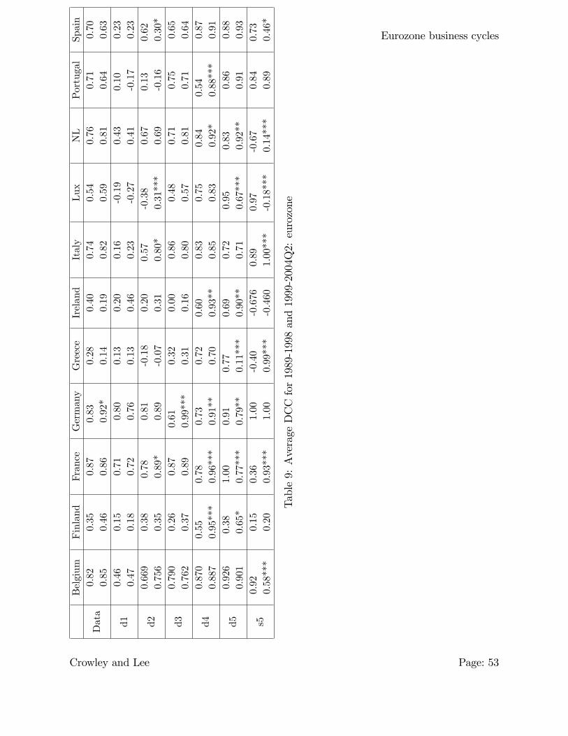
Eurozone business cycles
Belgium
Finland
France
Germany
Greece
Ireland
Italy
Lux
NL
Portugal
Spain
Data
0.82
0.85
0.35
0.46
0.87
0.86
0.83
0.92*
0.28
0.14
0.40
0.19
0.74
0.82
0.54
0.59
0.76
0.81
0.71
0.64
0.70
0.63
d10.46
0.47
0.15
0.18
0.71
0.72
0.80
0.76
0.13
0.13
0.20
0.46
0.16
0.23
-0.19
-0.27
0.43
0.41
0.10
-0.17
0.23
0.23
d20.669
0.756
0.38
0.35
0.78
0.89*
0.81
0.89
-0.18
-0.07
0.20
0.31
0.57
0.80*
-0.38
0.31***
0.67
0.69
0.13
-0.16
0.62
0.30*
d30.790
0.762
0.26
0.37
0.87
0.89
0.61
0.99***
0.32
0.31
0.00
0.16
0.86
0.80
0.48
0.57
0.71
0.81
0.75
0.71
0.65
0.64
d40.870
0.887
0.55
0.95***
0.78
0.96***
0.73
0.91**
0.72
0.70
0.60
0.93**
0.83
0.85
0.75
0.83
0.84
0.92*
0.54
0.88***
0.87
0.91
d50.926
0.901
0.38
0.65*
1.00
0.77***
0.91
0.79**
0.77
0.11***
0.69
0.90**
0.72
0.71
0.95
0.67***
0.83
0.92**
0.86
0.91
0.88
0.93
s50.92
0.58***
0.15
0.20
0.36
0.93***
1.00
1.00
-0.40
0.99***
-0.676
-0.460
0.89
1.00***
0.97
-0.18***
-0.67
0.14***
0.84
0.89
0.73
0.46*
Table9:AverageDCCfor1989-1998and1999-2004Q2:eurozone
Crowley and Lee Page: 53
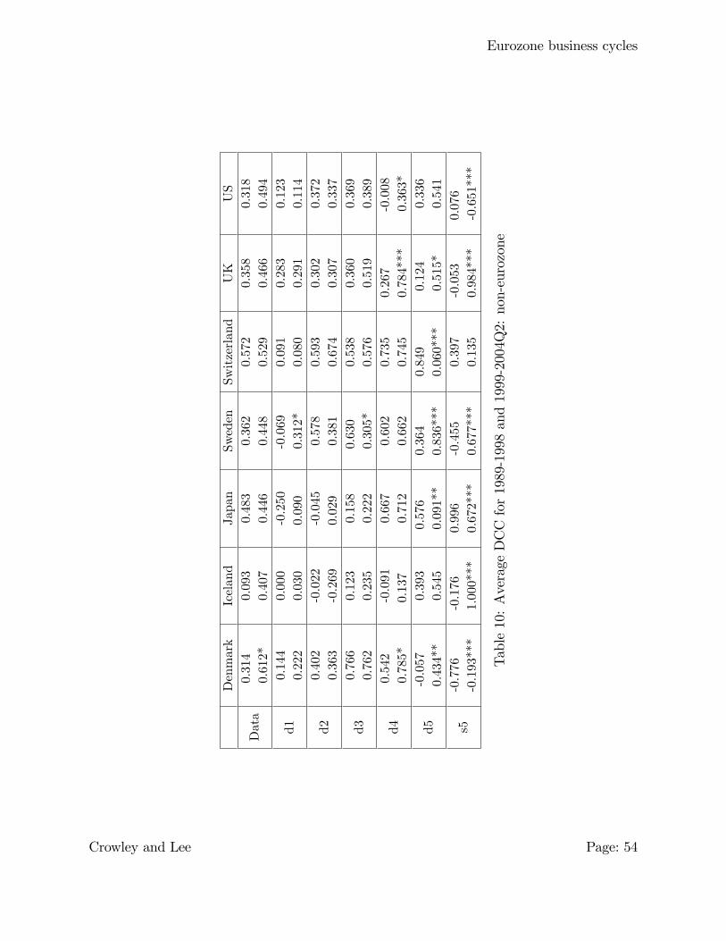
Eurozone business cycles
Denmark
Iceland
Japan
Sweden
Switzerland
UK
US
Data
0.314
0.612*
0.093
0.407
0.483
0.446
0.362
0.448
0.572
0.529
0.358
0.466
0.318
0.494
d10.144
0.222
0.000
0.030
-0.250
0.090
-0.069
0.312*
0.091
0.080
0.283
0.291
0.123
0.114
d20.402
0.363
-0.022
-0.269
-0.045
0.029
0.578
0.381
0.593
0.674
0.302
0.307
0.372
0.337
d30.766
0.762
0.123
0.235
0.158
0.222
0.630
0.305*
0.538
0.576
0.360
0.519
0.369
0.389
d40.542
0.785*
-0.091
0.137
0.667
0.712
0.602
0.662
0.735
0.745
0.267
0.784***
-0.008
0.363*
d5-0.057
0.434**
0.393
0.545
0.576
0.091**
0.364
0.836***
0.849
0.060***
0.124
0.515*
0.336
0.541
s5-0.776
-0.193***
-0.176
1.000***
0.996
0.672***
-0.455
0.677***
0.397
0.135
-0.053
0.984***
0.076
-0.651***
Table10:AverageDCCfor1989-1998and1999-2004Q2:non-eurozone
Crowley and Lee Page: 54
Eurozone business cycles
Tables 9 and 10 yield some striking and intriguing results. First, there has been no
signi�cant increase in correlation for eurozone member states between the two periods,
with the exception of Germany, which perhaps might be expected given that the shock of
reuni�cation falls into the prior period. In fact, correlations for Greece, Ireland, Portugal
and Spain fell in the post-EMU inception period. Outside the eurozone, Denmark was the
only country to experience a signi�cant increase in correlation, although correlations did
rise for all other countries outside the eurozone with the exception of Japan, again which
might be anticipated. This is likely once again due to the international synchronisation
of turning points in business cycles observed earlier, given the generalised slowdown in
economic growth for industrialised countries in the period since 1999.
Once the data is decomposed by frequency of growth cycle though, a somewhat di¤erent
picture emerges. Finland, for example, has an insigni�cant increase in its overall correla-
tion, but the 2-4 year growth cycles have become much more correlated with the eurozone,
and the 4-8 year growth cycles are also more correlated. France also has some intriguing
results, as there is virtually no overall correlation change, but the 2-4 year growth cycle
and cycles longer than 8 years are now signi�cantly more correlated, while the 4-8 year
cycle is signi�cantly less correlated with the eurozone. Given the similarity of the French
and German business cycles, the directions in the movement of correlations for the Ger-
man growth cycle correlations are similar to those of France, except that now it is obvious
that the increase in overall German correlations have been caused by an increase in the
correlations of cycles at a 1-2 year growth cycle frequency. In the case of Greece, we know
that the energy is not as heavily concentrated in the wavelet smooth as for other countries
(see table 4), so that even though the s5 crystal is much more highly correlated with the
eurozone, the fall in the 4-8 year growth cycle correlation dominates, giving an overall fall
in correlation.
As business cycle frequencies are to be found in the d4 and d5 crystals, it is interesting
to note that in all member states in the eurozone (the exception being Greece) the d4 corre-
lation increased, and signi�cantly so in Finland, France, Germany, Ireland, the Netherlands
and Portugal. For non-eurozone countries, this increase in correlation for the d4 crystal is
also true in all cases, but only signi�cantly so for Denmark, the UK and the US. For the
d5 crystal, correlation increased signi�cantly for Finland, Ireland, the Netherlands for the
eurozone member states, although it decreased signi�cantly for France, Germany, Greece
and Luxembourg. For the non-eurozone member states, there was a signi�cant increase
in correlation for Denmark, Sweden and the UK, which suggests that the establishment of
Crowley and Lee Page: 55
Eurozone business cycles
the euro has had an impact on economies outside of the eurozone area. Clearly unless we
know the frequency at which business cycles occurred in each member state, it is di¢ cult to
make any judgement about whether there has been further convergence since the inception
of EMU, but even without knowing this, we can state35 that there appears to have been a
signi�cant convergence of business cycles with the eurozone for Finland, Ireland, and the
Netherlands, and for non-eurozone countries, there has only been signi�cant convergence
with the eurozone business cycle for Denmark.
6 Conclusions
In this paper we have studied the co-movement of GDP growth cycles for a set of European
member states and other industrialized countries against that of the eurozone using wavelet
time-frequency analysis. This decomposed quarterly real GDP data to obtain series ac-
cording to di¤erent ranges of cycle frequencies (or crystals), which correspond to growth
cycles at di¤erent frequency ranges. Using these crystals a static variance and correlation
analysis of the crystals was conducted, and then the crystals were used in a GARCH-DCC
model to obtain dynamic conditional correlations for growth cycles against their eurozone
counterpart.
The conclusions are as follows:
a) as most of the variables contained higher energy in the wavelet smooth than in the
detail crystals, the multiresolution decomposition analysis con�rmed the �ndings of
Granger (1966) and Levy and Dezhbakhsh (2003b) that most energy in economic
series can be found in longer term �uctuations, based on the shape of the generalized
spectrum for economic variables.
b) con�ning the analysis to cycles of less than 8 years, several di¤erent growth cycles
consistently appear in the data, notably at several frequencies above the 2 quarter
periodicity, some of which contain signi�cant energy as compared with the conven-
tionally measured business cycle. This con�rms and extends the notion of growth
cycles originally proposed by Zarnovitz (1985) and analysed by Kontolemis (1997)
for the G7 and Zarnowitz and Ozyildirim (2002) for the US. To date, most business
cycle research has concentrated on the conventionally-measured business cycle, but
clearly several growth cycles at di¤erent frequencies are also at work.35This is by assuming that if there is a signi�cant increase in correlation for both the d4 and d5 crystals,
then there must be convergence in growth cycles at this frequency.
Crowley and Lee Page: 56
Eurozone business cycles
c) the MODWT analysis showed that since the 1970s and 1980s the energy contained
in the d1 and d2 crystals (cycles lasting less than one year) has waned, but that
relatively more energy is now located in the d3 and d4 (1-4 year cycles) crystals.
d) the MODWT analysis also suggested that recessions appear to occur because of a
coincident dip in growth cycles at all frequencies;
e) the static wavelet variance analysis showed that apart from Germany and France,
most EU member states have variances for di¤erent frequency cycles that are above
eurozone variances. Also, it was noted that eurozone variances by scale lie above
those for the US, which may be due to o¤setting asymmetric shocks. A test was also
conducted for homogeneity of variance through time for each crystal, and this was
found not to be the case for the high frequency detail crystals, but most low frequency
detail crystals possessed variance homogeneity.
f) the static wavelet correlation analysis showed that EU member states roughly fall into
one of 4 categories, with high and signi�cant correlations for France, Germany and
Belgium, but a low number of signi�cantly positive correlations for Finland, Greece,
Ireland, Sweden and the UK).
g) The static co-correlation analysis categorized the EUmember states into three groups,
with most eurozone member states being highly synchronised against the eurozone
aggregate, but some member states were not synchronised against the eurozone either
at higher (Greece and Ireland) or lower frequencies (Denmark, Sweden, UK).
h) dynamic conditional correlation coe¢ cients showed that for all crystals, correlations
were signi�cantly positive for most of the time for France, Germany and Belgium,
but that for other crystals, correlations were not always signi�cantly positive. The
correlations for Greece and Ireland were particularly worrysome, as there were periods
during which the correlations were signi�cantly negative against the eurozone.
i) analysis of convergence in the dynamic correlation of the growth cycles revealed that
there has been no signi�cant increase in the overall correlation of eurozone member
states before and after EMU, with the exception of Germany. However, when the
analysis is repeated at business cycle frequencies, it appears that signi�cant conver-
gence with the eurozone can be con�rmed since 1999 for Finland, Ireland, and the
Netherlands; and for non-eurozone countries, only Denmark has converged.
Crowley and Lee Page: 57
Eurozone business cycles
Further research is obviously needed here, as this methodology clearly opens up new
avenues of research. One of the mysteries of the frequency domain literature is the existence
of very long cycles in the data, that are obviously being picked up by spectral analysis. With
long enough series, wavelet analysis might be able to separately "resolve" these long cycles
in the data, and identify their approximate periodicity. The second question that springs
to mind is "what is driving these growth cycles?" Clearly, more analysis could be done
with the crystals for each country to shed some light on the factors driving these growth
cycles, now that they have been detected and properly resolved by the methodology used
here.
Crowley and Lee Page: 58
Eurozone business cycles
Appendices
A Euro area business cycle chronology
The euro area business cycle dating committee only make an announcement when they
think there has been a de�nite new trough. They have not recently meet formally, but are
in contact on a regular basis to review economic data as it appears, both leading (such as
http://www.cepr.org/data/EuroCOIN/latest/) and trailing indicators.
The decision the committee reached when it met in 2003 was as follows:
" Euro area GDP has slowed down since the �rst quarter of 2001. A weak resurgence
of positive growth at the beginning of 2002 seems to have come to a new halt. Employ-
ment has grown somewhat, while industrial production, after having fallen sharply in 2001,
shows weak signs of recovery. Investment has been declining for more than two years, but
government consumption rose 2.2% in 2001 and 2.7% in 2002.
Qualitatively, the recent behavior of GDP resembles that of the 1980s recession. Employ-
ment, however, is not declining. Based on currently available data, our current judgment
is therefore that the euro area has been experiencing a prolonged pause in the growth of
economic activity, rather than a full-�edged recession. "
So for the purpose of this study, euro area recessions are given as: 1974q3 to 1975q1,
1980q1 to1982q3, and 1992q1 to 1993q3.
Crowley and Lee Page: 59
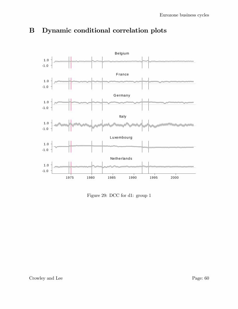
Eurozone business cycles
B Dynamic conditional correlation plots
1.0
1.0
1.0
1.0
1.0
1.0
1.0
1.0
1.0
1.0
1.0
1.0
1975 1980 1985 1990 1995 2000
Belgium
France
Germany
Ita ly
Luxembourg
Nether lands
Figure 29: DCC for d1: group 1
Crowley and Lee Page: 60
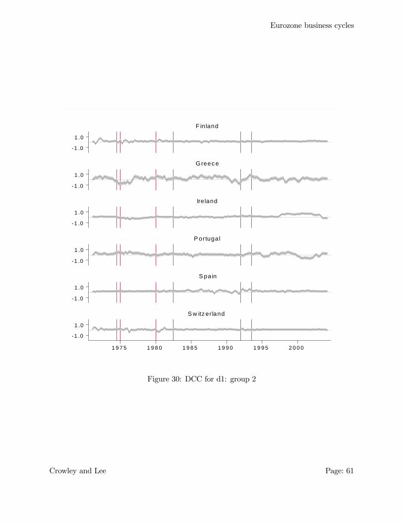
Eurozone business cycles
1 .0
1 .0
1 .0
1 .0
1 .0
1 .0
1 .0
1 .0
1 .0
1 .0
1 .0
1 .0
1 9 7 5 1 9 8 0 1 9 8 5 1 9 9 0 1 9 9 5 2 0 0 0
F inland
G reec e
Ire land
P ortugal
S pain
S w itz er land
Figure 30: DCC for d1: group 2
Crowley and Lee Page: 61
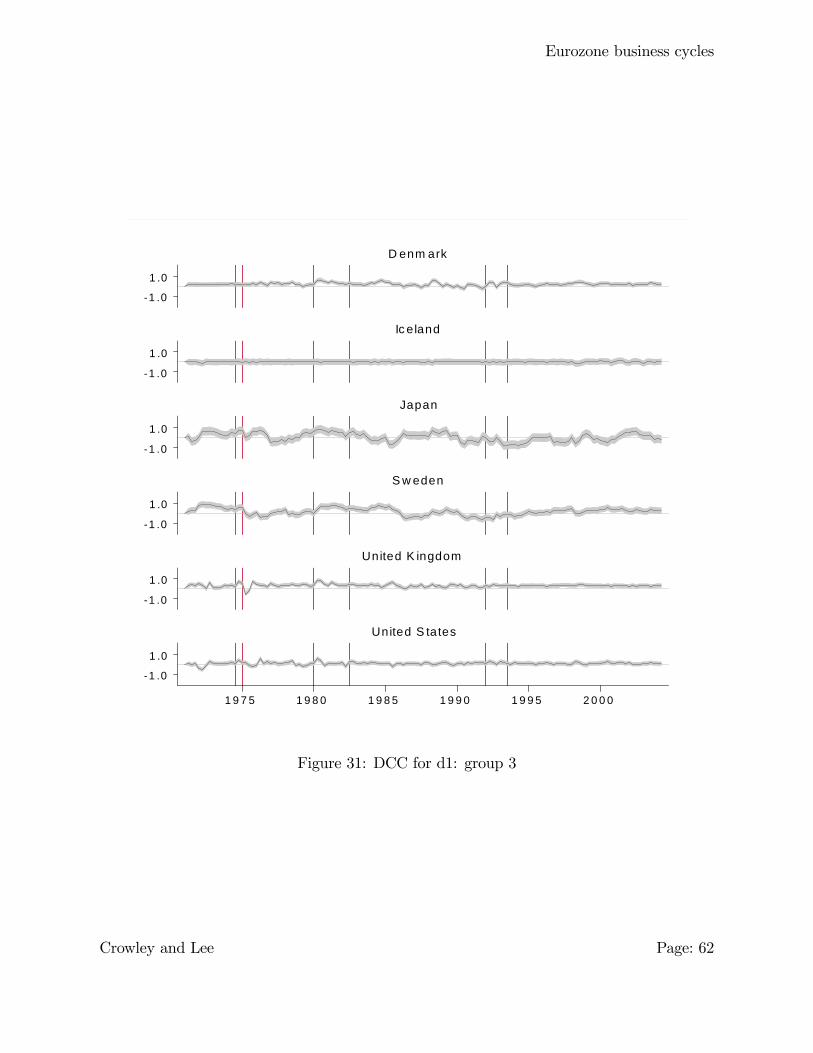
Eurozone business cycles
1 .0
1 .0
1 .0
1 .0
1 .0
1 .0
1 .0
1 .0
1 .0
1 .0
1 .0
1 .0
1 9 7 5 1 9 8 0 1 9 8 5 1 9 9 0 1 9 9 5 2 0 0 0
D enm ark
Ic eland
Japan
S w eden
United K ingdom
United S tates
Figure 31: DCC for d1: group 3
Crowley and Lee Page: 62
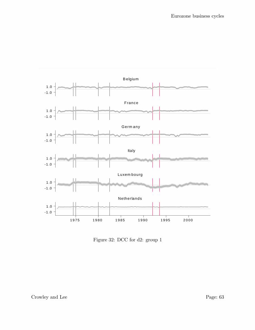
Eurozone business cycles
1 .0
1 .0
1 .0
1 .0
1 .0
1 .0
1 .0
1 .0
1 .0
1 .0
1 .01 .0
1 9 7 5 1 9 8 0 1 9 8 5 1 9 9 0 1 9 9 5 2 0 0 0
B elgium
France
Germ any
Ita ly
Luxem bourg
Nether lands
Figure 32: DCC for d2: group 1
Crowley and Lee Page: 63
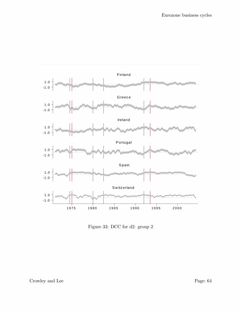
Eurozone business cycles
1 .0
1 .0
1 .01 .0
1 .0
1 .0
1 .0
1 .0
1 .01 .0
1 .01 .0
1 9 7 5 1 9 8 0 1 9 8 5 1 9 9 0 1 9 9 5 2 0 0 0
F inland
Greec e
Ireland
P ortugal
S pain
S w itz erland
Figure 33: DCC for d2: group 2
Crowley and Lee Page: 64
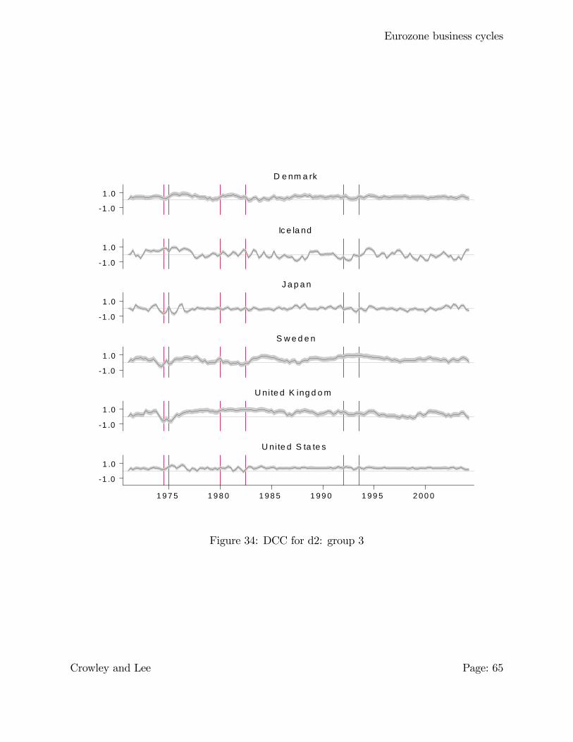
Eurozone business cycles
1 .0
1 .0
1 .0
1 .0
1 .0
1 .0
1 .0
1 .0
1 .0
1 .0
1 .0
1 .0
1 9 7 5 1 9 8 0 1 9 8 5 1 9 9 0 1 9 9 5 2 0 0 0
D e nm a rk
Ic e la nd
J a p a n
S w e d e n
U nite d K ing d o m
U nite d S ta te s
Figure 34: DCC for d2: group 3
Crowley and Lee Page: 65
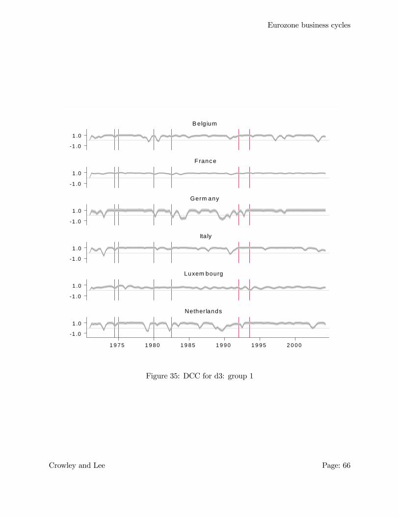
Eurozone business cycles
1 .0
1 .0
1 .0
1 .0
1 .0
1 .0
1 .0
1 .0
1 .0
1 .0
1 .0
1 .0
1 9 7 5 1 9 8 0 1 9 8 5 1 9 9 0 1 9 9 5 2 0 0 0
B elgium
France
Germ any
Ita ly
Luxem bourg
Nether lands
Figure 35: DCC for d3: group 1
Crowley and Lee Page: 66
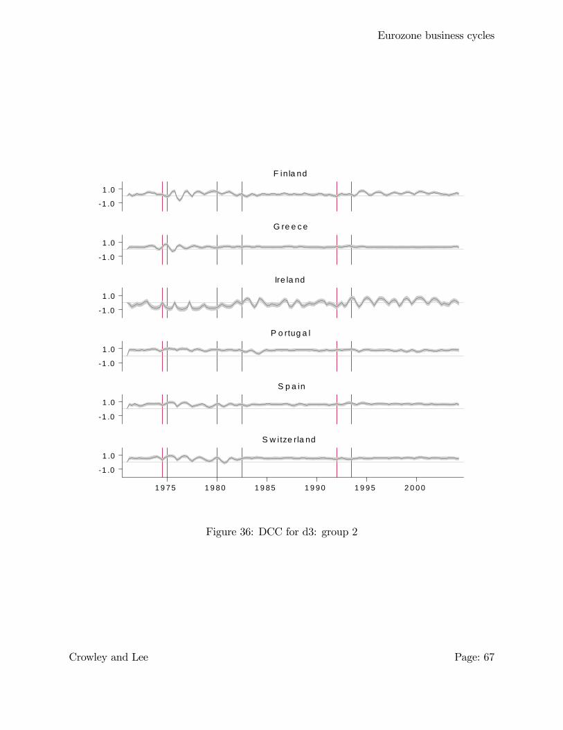
Eurozone business cycles
1 .0
1 .0
1 .0
1 .0
1 .0
1 .0
1 .0
1 .0
1 .0
1 .0
1 .0
1 .0
1 9 7 5 1 9 8 0 1 9 8 5 1 9 9 0 1 9 9 5 2 0 0 0
F in la nd
G re e c e
Ire la nd
P o rtug a l
S p a in
S w itze rla nd
Figure 36: DCC for d3: group 2
Crowley and Lee Page: 67
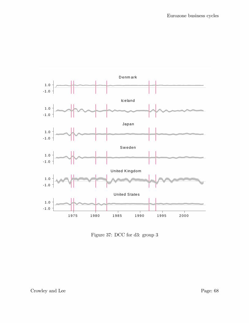
Eurozone business cycles
1 .0
1 .0
1 .0
1 .0
1 .0
1 .0
1 .0
1 .0
1 .0
1 .0
1 .0
1 .0
1 9 7 5 1 9 8 0 1 9 8 5 1 9 9 0 1 9 9 5 2 0 0 0
D enm ark
Ic eland
Japan
S w eden
United K ingdom
United S tates
Figure 37: DCC for d3: group 3
Crowley and Lee Page: 68
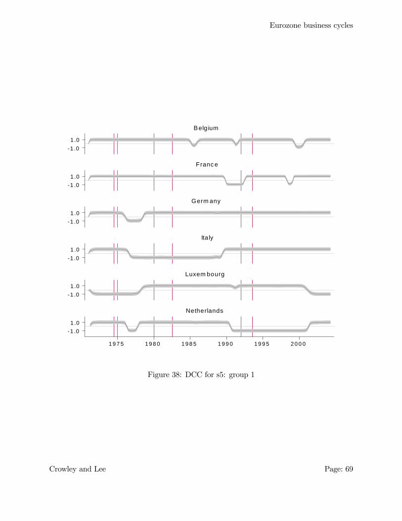
Eurozone business cycles
1 .01 .0
1 .01 .0
1 .01 .0
1 .01 .0
1 .01 .0
1 .01 .0
1 9 7 5 1 9 8 0 1 9 8 5 1 9 9 0 1 9 9 5 2 0 0 0
B elgium
Franc e
Germ any
Ita ly
Luxem bourg
Netherlands
Figure 38: DCC for s5: group 1
Crowley and Lee Page: 69
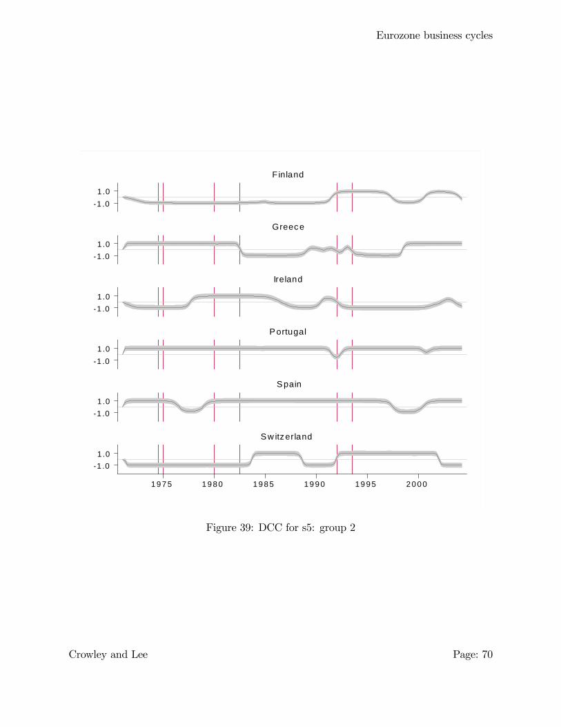
Eurozone business cycles
1 .01 .0
1 .01 .0
1 .01 .0
1 .01 .0
1 .01 .0
1 .01 .0
1 9 7 5 1 9 8 0 1 9 8 5 1 9 9 0 1 9 9 5 2 0 0 0
Finland
Greece
Ireland
P ortugal
S pain
S w itzerland
Figure 39: DCC for s5: group 2
Crowley and Lee Page: 70
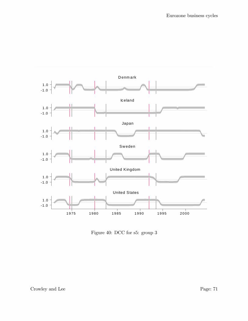
Eurozone business cycles
1 .01 .0
1 .01 .0
1 .01 .0
1 .01 .0
1 .01 .0
1 .01 .0
1 9 75 1 9 80 1 9 85 1 9 90 1 9 95 2 0 00
D enm ark
Iceland
Japan
Sw eden
United K ingdom
United States
Figure 40: DCC for s5: group 3
Crowley and Lee Page: 71
Eurozone business cycles
References
Agresti, A. and B. Mojon (2001, December). Some stylised facts on the euro area business
cycle. Technical Report 95, ECB.
A�Hearn, B. and U. Woitek (2001). More international evidence on the historical prop-
erties of business cycles. Journal of Monetary Economics 47, 321�346.
Altavilla, C. (2004). Do EMU members share the same business cycle? Journal of Com-
mon Market Studies 42 (5), 869�896.
Ambler, S., E. Cardia, and C. Zimmerman (2004). International business cycles: What
are the facts? Journal of Monetary Economics 51, 257�276.
Artis, M. and W. Zhang (1997). International business cycle and the ERM: Is there a
european business cycle? International Journal of Finance and Economics 2, 1�16.
Artis, M. and W. Zhang (1999). Further evidence on the international business cycle and
the ERM: Is there a european business cycle? Oxford Economic Papers 51, 120�132.
Backus, D. and P. Kehoe (1992). International evidence on the historical properties of
business cycles. American Economic Review 82, 864�888.
Backus, D., P. Kehoe, and F. Kydland (1992). International real business cycles. Journal
of Political Economy 101, 745�775.
Backus, D., P. Kehoe, and F. Kydland (1995). International business cycles: Theory
and evidence. In F. Cooley (Ed.), Frontiers of Businss Cycle Research, pp. 331�356.
Princeton, NJ, USA: Princeton University Press.
Basu, S. and A. Taylor (1999). Business cycles in international historical perspective.
Journal of Economic Perspectives 13 (2), 45�68.
Baxter, M. and M. Kouparitsas (2004, August). Determinants of business cycle comove-
ment: A robust analysis. Working Paper 10725.
Bergman, M., M. Bordo, and L. Jonung (1998, September). Historical evidence on busi-
ness cycles: The international experience. In J. Fuhrer and S. Schuh (Eds.), Beyond
Shocks: What Causes Business Cycles, Working Paper Series in Economics and Fi-
nance, Boston, MA, USA, pp. 65�113. Federal Reserve Bank of Boston.
Bruce, A. and H.-Y. Gao (1996). Applied Wavelet Analysis with S-PLUS. New York, NY,
USA: Springer-Verlag.
Crowley and Lee Page: 72
Eurozone business cycles
Canova, F. and G. de Nicoló (2003). On the sources of business cycles in the g-7. Journal
of International Economics 59, 77�100.
Comin, D. and M. Gertler (2003, September). Medium term business cycles. Technical
Report 10003, NBER, Cambridge, MA, USA.
Constantine, W. and D. Percival (2003, October). S+Wavelets 2.0.
Crivellini, M., M. Gallegati, M. Gallegati, and A. Palestrini (2004). Industrial output
�uctuations in developed countries: A time-scale decomposition analysis. Technical
report, European Commission, Brussels, Belgium. Working Papers and Studies: Pa-
pers from the 4th Eurostat and DGFin Colloquium "Modern Tools for Business Cycle
Analysis".
Croux, C., M. Forni, and L. Reichlin (2001). A measure of comovement for economic
variables: Theory and empirics. The Review of Economics and Statistics 83 (2), 232�
241.
Crowley, P. (2005, January). An intuitive guide to wavelets for economists. Technical
Report forthcoming, Bank of Finland. Discussion paper series.
De Haan, J., R. Inklaar, and O. Sleijpen (2002). Have business cycles become more
synchronized? Journal of Common Market Studies 40 (1), 23�42.
Debauchies, I. (1992). Ten Lectures on Wavelets. Montpelier, VT, USA: Capital City
Press.
Duarte, A. and K. Holden (2003). The business cycle in the g-7 economies. International
Journal of Forecasting 19, 685�700.
Engle, R. (2002). Dynamic conditional correlation - a simple class of multivariate GARCH
models. Journal of Business and Economic Statistics 20 (3), 339�50.
Engle, R. and K. Sheppard (2001). Theoretical and empirical properties of dynamic con-
ditional correlation multivariate GARCH. Technical Report Discussion paper 2001-15,
University of California, San Diego, CA, USA.
Fagan, G., J. Henry, and R. Mestre (2001, January). An area-wide model (AWM) for the
euro area. Technical Report 42, ECB. Working paper.
Frankel, J. and A. Rose (2002). An estimate of the e¤ect of common currencies on trade
and income. Quarterly Journal of Economics 117, 437�466.
Crowley and Lee Page: 73
Eurozone business cycles
Garrison, R. (2001). Time and Money: The Macroeconomics of Capital Structure. Lon-
don, UK: Routledge.
Gençay, R., F. Selçuk, and B. Whicher (2001). An Introduction to Wavelets and Other
Filtering Methods in Finance and Economics. San Diego, CA, USA: Academic Press.
Granger, C. (1966). The typical spectral shape of an economic variable. Economet-
rica 34 (1), 150�161.
Greenhall, C. (1991). Recipes for degrees of freedom of frequency stability estimators.
IEEE Transactions on Instrumentation and Measurement 40, 994�9.
Hamilton, J. (1989). A new approach to the eonomic analysis of nonstationary time series
and the business cycle. Econometrica 57 (2), 357�384.
Harding, D. and P. A. (2002). Dissecting the cycle: A methodological investigation.
Journal of Monetary Economics 49 (2), 365�81.
Helpman, E. and P. Krugman (1985). Market Structure and Foreign Trade. Cambridge,
MA, USA: MIT Press.
Hicks, J. (1950). A Contribution to the Theory of the Trade Cycle. Oxford, UK: Oxford
University Press.
Inclan, C. and G. Tiao (1994). Use of cumulative sums of squares for retrospective de-
tection of changes of variance. Journal of the American Statistical Association 89,
913�923.
Keynes, J. (1936). The General Theory of Employment, Interest and Money. London,
UK: Macmillan.
Kitchin, J. (1923). Cycles and trends in economic factors. Review of Economics and
Statistics 5, 10�17.
Kontolemis, Z. (1997). Does growth vary over the business cycle? some evidence from
the g7 countries. Economica 64 (255), 441�460.
Krugman, P. (1991). Geography and Trade. Cambridge, MA, USA: MIT Press.
Kuznets, S. (1958). Long swings in the growth of population and in related economic
variables. Proceedings of the American Philosophical Society 102, 25�57.
Leamer, E. (1983). Let�s take the con out of econometrics.American Economic Review 73,
31�43.
Crowley and Lee Page: 74
Eurozone business cycles
Levy, D. and H. Dezhbakhsh (2003a). International evidence on output �uctuation and
shock persistence. Journal of Monetary Economics 50, 1499�1530.
Levy, D. and H. Dezhbakhsh (2003b). On the typical spectral shape of an economic
variable. Applied Economic Letters 10 (7), 417�423.
Lucas, R. (1977). Understanding business cycles. In K. Brunner and A. Meltzer (Eds.),
Stabilization of the Domestic and International Economy, Volume 5, pp. 7�29.
Mallat, S. (1989). A theory for multiresolution signal decomposition: The wavelet repre-
sentation. IEEE Transactions on Pattern Analysis and Machine Intelligence 11 (7),
674�693.
Mir, A. and D. Osborn (2004, May). Seasonal adjustment and the detection of business
cycle phases. Technical Report Working Paper 357, ECB, Frankfurt, Germany.
Mitchell, W. (1946). Business cycles: The problem and its setting. New York, USA.
Morgenstern, O. (1959). International Financial Transactions and Business Cycles.
Princeton, NJ, USA: Princeton University Press.
Percival, D. and H. Mofjeld (1997). Analysis of subtidal coastal sea level �usctuations
using wavelets. Journal of the American Statistical Association 92, 868�80.
Percival, D. and A. Walden (2000). Wavelet Methods for Time Series Analysis. Cam-
bridge, UK: Cambridge University Press.
Sensier, M., M. Artis, D. Osborn, and C. Birchenhall (2004). Domestic and international
in�uences on business cycle regimes in europe. International Journal of Forecast-
ing 20, 343�357.
Sichel, D. (1993). Business cycle asymmetry: A deeper look. Economic Inquiry 31, 224�
236.
Valle e Azevedo, J. (2002, April). Business cycles: Cyclical comovement within the euro-
pean union in the period 1960-1999. a frequency domain approach. Technical Report
WP 5-02, Banco do Portugal.
Whitcher, B., S. Byers, P. Guttorp, and D. Percival (1998). Testing for homogeneity of
variance in time series: Long memory, wavelets and the nile river. Technical Report
Technical Report 9, National Research Center for Statistics and the Environment.
Whitcher, B., P. Guttorp, and D. Percival (1999). Mathematical background for wavelet
estimators of cross-covariance and cross-correlation. Technical Report TSE No. 038,
Crowley and Lee Page: 75
Eurozone business cycles
NRCSE.
Whitcher, B., P. Guttorp, and D. Percival (2000). Wavelet analysis of covariance with
application to atmospheric time series. Journal of Geophysical Research 105 (D11),
14,941�14,962.
Zarnovitz, V. (1985). Recent work on business cycles in historical perspective: A review
of theories and evidence. Journal of Economic Literature 23, 523�80.
Zarnowitz, V. and A. Ozyildirim (2002, January). Time series decomposition and mea-
surement of business cycles, trends and growth cycles. Technical Report 8736, NBER,
Cambridge, MA, USA.
Crowley and Lee Page: 76