DECOMPOSING THE GIN1 COEFFICIENT TO REVEAL … · DECOMPOSING THE GIN1 COEFFICIENT TO REVEAL THE VERTICAL, HORIZONTAL, AND RERANKING EFFECTS OF INCOME TAXATION 1. RICHARD ... income

DECOMPOSING THE GIN1 COEFFICIENT TO REVEAL THE VERTICAL, HORIZONTAL, AND RERANKING EFFECTS OF INCOME TAXATION 1. RICHARD ARONSON* & PETER J. LAMBERT**

Abstract - Taxes may treat equals un- equally, they may treat unequals un- equally, and they may cause the ranking of people from poor to rich to be different post-tax than it was pretax. This paper offers geometric and mathematical techniques for measuring and computing the above three effects. They are referred to as the vertical, horizontal, and reranking effects. Several scholars current/y equate the reranking effect with horizontal inequity. We show, however, that the reranking effect is separate and distinct from the traditional concept of horizontal equity. Our measures are derived by comparing the pretax and posttax Gini coefficients and decomposing the total redistributive effect of the tax. We compare our method to others and provide some preliminary empirical estimates for the income taxes used in the United Kingdom and Italy. For the United Kingdom and Italy, vertical effects dominate horizontal and reranking effects. However, we sus-

*Department of Economics, Lehigh Unwerstty. Bethlehem, PA 18015 **Department of Economtcs, University of York, Heslmgton, York YOl 5DD. England

pect that for the United States income tax the horizontal and reranking effects will have greater relative importance.

INTRODUCTION

Taxes and tax systems are judged on three essential features: how much revenue they raise; how much excess burden or distortion they create; and whether or not they meet the accepted criteria of equity and fairness. We concentrate on the fairness issue and offer measures that can be employed in monitoring the equity characteristics of a tax or tax system over time or in comparing the equity features of alternative tax systems at a point in time. Our measurements are made by decomposing the Gini coefficient associated with the posttax income distribution and comparing this with the pretax Gini. This technique reveals normatively significant and commensurable measures of the vertical, horizontal, and reranking effects of income taxation, and thereby builds on the previous work of Atkinson (1980), Plotnick (1981,

273

1985), Berliant and Strauss (1985, 1993), Jenkins (1988a, 1988b, 1988c), Berglas (1971), Reynolds and Smolensky (1977), and Kakwani (1984).

The Equity Issue

The equity characteristrc of a tax IS usually separated into horizontal and vertical components Horizontal equity (HE) is a normative goal that calls for the equal treatment of equals; vertical equity (VE) is another ethical norm refernng to the treatment of unequals As simple as they sound, these criteria are difficult to ap ply. There are both theoretical and practical problems. For example, there is concern that HE and VE! are not rnde- pendent criteria. Recent discussion In this journal by Louis Kaplow (1989) questions the significance of the HE command. Kaplow points out that defining equality groups is at best difficult and even when done there may be little to justify the pretax distribution of in come. Moreover, as the space between income equality groups diminishes, the significance of HE blurs In the shadow of VE. For Kaplow, HE exists as a by- product in an attempt ‘to achieve VE.

Musgrave 1(1990), on the other hand, emphasizes the significance of HE. HE is not merely a mathematical condition needed to achieve Pigovian minimum aggregate sacrifice; rather, it is a robust rule of fairness that is contained tn vir tually all constructs of drstributrve justice. However, Musgrave is tnostly concerned with the potential trade-off between HE and VE in a second-best world. How can society judge a tax reform proposal that improves HE at the expense of VE?

A method of coprng with the HE mea.. surement problem has been offered by Atkinson (1980) aInd Plotnick (1981). Their insight is that horizontal equity, classically defined as the equal treatment of equals, must be violated if the income ranking (from poor to rich) of rndi-

viduals IO altered by the distribution of taxes. As a result, they define the amount of horizontal inequity as a concentration Index measure of the difference between the posttax distribution of Income using a posttax ranking of individuals and the posttax drstnbution of Income iusing the pretax ranking of rndi- viduals. The technique we devise in this paper c;iptures this rerankrng effect but Identifies rt as a component separate from horizontal equity, classrcally defined. That IS, we compare the pretax with, the posttax distributron of income and decompose the total redistributive effelct of the tax into three components

V =z tl-re redistribution that would have occurred If equals had been treated equally.

H = tne loss Iof the redrstributive effect accounted for by the unequal treatment of equals, a direct measure of horizontal inequity classically defined.

R = a further subtraction arising from the difference iIn pretax ancl posttax rankings of income units.

In what follows, we show how to measure V, Y, and R commensurably. First, we provide some historical perspective on the rneasurement problem and explain our method in geometric terms. The next section conta;ins the mathemat- ICS of the technique and a simple application. We also compare our measures to those of other investigators and explain why we believe our techniques have normative as well as descriptive value. Later, we present and discuss ini- tial emprrical estimates of V, H, and R using the United Kingdom and Italian income taxes as examples.

HISTORICAL PERSPECTIVE AND GEO- METRIC MODEL

A popular device for measuring the re- drstrrbutive effect of taxes is the Lorenz

I DECOMPOSING THE GINI COEFFICIENT

curve and the Grni coefficient calculated from it. Indeed, Pechman and Okner (1974) in their classic tax Incidence study used Gini coefficients to describe the redistributive impact of taxation in the United States. But care must be exer- cised here, especially if there is a desire to separate the horizontal from the vertical effects of a tax. Anthony Atkinson (1980) and Robert Plotnick (1981) have shown that a simple comparison of a pretax and posttax distribution of tn- come might not reveal the magnitude of the horizontal effect of a tax. Plotnick, therefore, suggests a very interesting technique for separating the horizontal from the vertical effects. The technique is shown below and provides a conve- nient starting point for the explanation of our own method.

Plotnick and others accept the notion of horizontal equity as the “equal treatment of equals” but believe that “this norm also requires that rankings of all units should not be altered during the redistributive process” (Plotnick, 1981, p. 283; also see Feldstein, 1976, p. 123-24). It follows, therefore, that in

their view, horizontal inequities arise as a result of changes in rankings of economic units from pretax to posttax. The insight is described in Figure 1, where the cumulative percentage of economic units is measured along the horizontal axis and cumulative percent of income along the vertical axis. OB is the line of perfect equality (e.g., 30 percent of the economic units received 30 percent of the total income) and OAB, which is a line of less than perfect equality, is the pretax Lorenz curve. Geometrically, the Gini coefficient is the area between the line of perfect equality and the Lorenz curve (OBD-OABD) divided by the area of the triangle OBD.’

Suppose we now introduce a tax-rate structure that is aimed at reducing the differentials between the rich and poor,

and which results in a new Lorenz curve OA’B. Calculatron of the Gini coefficient would show that the distribution of income had become more equal and thus, in harmony with the desired goal. Plot- nick has pointed out, however, that the perceived improvement in vertical equity (reducing the difference between the rich and poor) may not represent a pure improvement because the ranking of economic units pretax and posttax might not be identical. Plotnick suggests draw- ing another concentration curve (the dashed line of Figure 1) that shows posttax income shares as a function of the pretax ranking of economic units, and proposes that a measure of horizontal inequity be based upon the area between the posttax concentration curve with a pretax ranking and the Lorenz curve with posttax ranking (i.e., between the dashed line and OA’B).

PlotnIck’s focusing on the importance of reranking in the distribution of income is a significant contribution to our understanding and interpretation of Gini coefficients. However, his defining horizontal equity as equivalent to the need to maintain the relative ranking of economic units also creates significant ambi- guities. The traditional concept of horizontal equity is simply the “equal treatment of equals” and thus, it follows that horizontal inequity is “unequal treatment of equals” (see Musgrave, 1959, p. 160; Pigou, 1960, p. 44; John- son and Mayer, 1962, p. 454; Berliant and Strauss, 1985). The concept, of course, requires that we identify a set of taxpayers we deem equal. Because the Plotnrck measure concerns itself only with relative rankings, and does not limit itself to measurements within an equality group, it unfortunately can give a false signal of horizontal inequity and, as a result, can confuse horizontal inequity with vertical equity.

Consider Figure 2, which shows the Lor-

I FIGURE 1

Cumuletlve % of Income

enz curve, OAB, for a two-person case in which one person IS poor and the other rich. Suppose the public sector is used to exactly reverse the posit tons of the two people. Now the rich person has the income of the poor and the poor person the income of the rich. The posttax Lorenz curve using an after tax ranking of economic units would be identical to the Lorenz curve of pretax income using the pretax ranking. The posttax concentration curve using the pretax ranking is, however, much different. It is OA’B, the mirror image of OAB. The problem is that under the Plotnick method, the area OA’BA would

Cumul $

Ive % of u Its

be ideniifred as one ot horizontal inequity even though ther are no equals to compare. Clearly the hange shown in Figure 2 represents a

-

hange between

unequals that is in th nature of a vertical change and must be taken into ac-

count as such if we ale to provide a complete picture of thle effects.” To our

way of thinking, as w such as Berliant and !

II as to others ‘5 rauss, it IS not a

measure of horizontal ~inequity, classically

defined.’

The model we now develop improves on the Plotnick technique by isolating the reranking of unequals effects (R) and


FIGURE 2

Cumulative 70 of Income

0

measuring it separately from both classical horizontal inequity (H) and the vertical effects (V) produced by a tax. In Ta- ble 1 we offer some simple arithmetic examples to aid in the explanation. Con- sider a set of six people divided into two subgroups. Three people (A,, A,, AJ are equally poor and three (B,, B2, BJ are equally rich. The incomes are given in column I of Table 1 and the Lorenz curve describing this distribution is shown as the solid curve OAB in Figure 3. The data in the middle portion of the table show the number of economic units and income in cumulative percent-

Cumulative % of Units

age terms. Column II of Table 1 shows the after tax distribution of income that would result from a 50 percent proportional tax on income. Notice that while such a tax generates $4,500 in revenue it does not change the relative distribution of income. The cumulative percentage distribution (middle part of Table 1) is exactly the same for both columns I and II, and thus, the Lorenz curve (solid curve) OAT3 is identical pretax and posttax. Casual observation shows that, in this case, the tax system has treated equals equally (I.e., there has been no horizontal effect), has maintained the

277

TABLE 1 HYPOTHETKAL PRETAX AND POSTTAX DlSTRlBUTlONS OF INCCjME

Income Before Tax income After Tax

I il III W IVa” V VI VlaC Vlld VW Vllb’

AI $1,000 $500 $450 $450 $400 $500 $600 A2 1,000 500 500 500 400 600 600 A3 1,000 500 550 550 400 700 600 BI 2,000 1,000 600 300 1,100 800 900 f32 2,000 1,000 1,000 1,000 1,100 900 900

ykome 2 000

$$ 1 000

84,500 1 400

$4,500 1,700 1,100

Total 84,500 I$00 900

Blr,soo $4,500 $4,500

$350 $567 550 567 800 567 500 933 800 933

1,500 933 94,500 84,5oa

17 33 50 67 83

100

Cumulative Percentage 11 11 IO 07 (10) 09 22 22 21 17 (21) 18 :.: :: 33 33 33 28 (33) i! 7 40 40 56 56 47 40 (40) 51 58 60 78 78 69 62 (62) 76 78 80

100 100 100 100 (100) 100 100 100

08 (08) (13) 19 (20) (29

31 (38) 50 (49) I:;; 67 (67) (79)

100 (100) (100)

Gini 0.167 0.167 0.233 0.322 0.233 0.130 0.256 (6 - GJg 0 -0.066 -0.155 --0.066 0.037 -0.089

Decomposition of (Gx G,,) V 0 0 0 --0.067 0.067 0.044 H 0 0.066 0.111 0 0.030 0.107 R 0 0 0.044 0 0 0.026

- - - P - P - _ - - - - - --..-

aThe cumulative percentages shown in the lower portion of column IV are based on the follobing poor to rich rank ordering of individuals: 13, Al A.2 A3 61 62. bThe cumulative percentages shown in the lower portion of column IVa are based on the following poor to rich rank ordering of individuals: A1 A2 A3 B1 B2 B3. ‘Column Vla shows the posttax distributton of income If within ea& group equals are taxed qqually and the total rev,. enue collected from each group is the same as in column VI. dThe cumulative percentages shown in the rniddle portion of column VII are based on the foljowing poor to rich rank ordering of individuals: A1 Bl AL A3 B2 B3. eThe cumulative percentages shown in the rniddle portion of column Vlla are based on the fqllowing poor to rich rank ordering of individuals: A1 A2 A3 B1 B2 B3. ‘Column Vllb shows the posttax distribution of income if within eaclrl group equals are taxed equally and the total revenue collected from each group IS the same as in column VII. The cumulative percentages /n the middle portion are based on the following rich to poor rank ordering of individuals: A1 A2 A3 B1 B2 !33. glGy - Gn) is the difference in value between the pretax Gin! coefficient and the Glni coefficient of the posttax distrl..

. I I

bution of-&come of the appropriate column

relative difference between rich and poor (i.e., there has been no vertical effect), and did not push a member of one subgroup into another (there is no Plotnick-type reranking).

Now consider the after tax income described in column III. The taxes Icollected from the six individuals are $550, $500, $450, $1,400, $1,000, and $600, re- spectively, so that. the total revenue collected remains $4.,500, or half the pretax income. People in the poor subgroup have, as a group, been taxed at 50 percent; so have people in the rich group. Thus, in a rough sense we still have a proportional tax rate structure and as a result there is no overall vertical effect.

Within each subgroup, however,, we have unequal treatment. The dashed Lorenz curve OAB in Figure 3 shows the after tax distribution of income, and when compared to thi solid curve, OAB isolates the change in income distribution asso&ated with the unequal treatment of equals. Indeed, the area between the dashed and solid lines measures the differenqe between the equal treatment of eqpals and the unequal treatment of eqbals. Thus, it can be [used as a measure’of horizontal inequity, that is, the horizontal effec:t among people with equal tax+paying capacity.

In the above example, there are no pre. tax and posttax ranking changes. Thus,


FIGURE 3

100

Cumulative % of Income 90

80

70

60

0 10 2.0 30 40 50 60 70

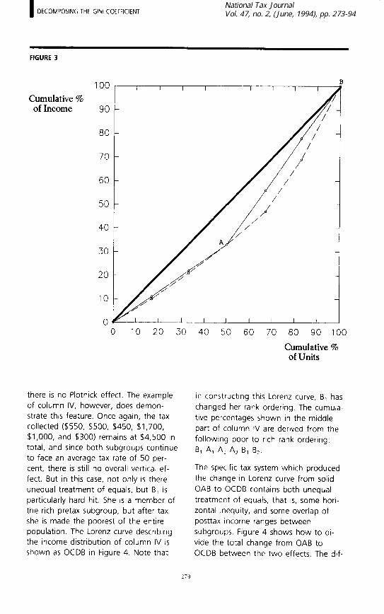
there is no Plotnick effect. The example of column IV, however, does demon- strate this feature. Once again, the tax collected ($550, $500, $450, $1,700, $1,000, and $300) remains at $4,500 in total, and since both subgroups continue to face an average tax rate of 50 percent, there is still no overall vertical effect. But in this case, not only is there unequal treatment of equals, but B, is particularly hard hit. She is a member of the rich pretax subgroup, but after tax she is made the poorest of the entire population. The Lorenz curve describing the income distribution of column IV is shown as OCDB in Figure 4. Note that

80 90 100


in constructrng this Lorenz curve, B, has changed her rank ordering. The cumulative percentages shown in the middle part of column IV are derived from the followlng poor to rich rank ordering:

B, A, A, A, B, ‘3,.

The specific tax system which produced the change in Lorenz curve from solid OAB to OCDB contains both unequal treatment of equals, that is, some horizontal Inequity, and some overlap of posttax income ranges between subgroups. Figure 4 shows how to di- vide the total change from OAB to OCDB between the two effects. The dif-

279

FIGURE 4

Cumulative % of Income

60

0 lo 20 30 40 50 60 70 80 90 Cumulative % of Units

ference between t.he solid line OAB and the dashed line connecting OEADB shows the horizontal effect. It represents the difference between the actual treatment of equals (dlashed OEADB) and the equal treament of equals (solid OAB). The cumulative percentages of column IVa show rhe posttax concentration curve usiny the pretax ranking of indl- viduals (i.e., the rank (ordering of indlvid- uals used to produce this concentration curve is A, A2 A3 B, &z BJ. The area between the dashed line OEADB and OCDB is yet to be identified. Simple observation SUggeSt5 it is not a vertical

chailge. This is because the overall tax on Iboth the rich and lhe poor groups remains 50 percent. Thus, since we have accounted for H and 1/ = 0, this remain-

ing area OCDAE must represent the amount of change in iinequality due to

reranking. That is, R is the difference between the Lorenz curve of the posttax distn but Ion of income i and the concentration curve showing the posttax dlstri-

bution of income using the pretax rank. Ing of individuals.

Column V and Figure 5 portray the distributional impact of a tax-rate ‘structurc:b


FIGURE 5

100

Cumulative % 9. of Income

80

70

60

50

40

30

20

10

0 0 IO 20 30 40 50 60 70 80 90 100


that is regressive but treats equals equally. In this case, the tax rate of the poor group is 60 percent, while that on the rich is 45 percent. With no unequal treatment of equals and no reranking, the entire change in the distribution of income (i.e., the area between Lorenz curves OAB and OA’B) is due to the unequal treatment of unequals. Thus, there is a vertical effect but neither a horizontal nor a reranking effect.

Figure 6 and columns VI and Vla show the decomposition when the tax system is progressive but unequal among equals. Here, the area between the solid

and dotted Lorenz curves OAB and OA’B shows the change in distribution that would occur as the result of a progressive tax that treated equals equally. The dotted Lorenz curve is based on the cumulative percentages shown in column Vla. However, the actual redistribution is less than that Indicated above because of the increased Inequality caused by the unequal treatment of equals (i.e., the area between the dotted and dashed Lorenz curves OA’B shows the amount of horizontal effect). In this example there is no reranking of individuals. Thus, R = 0.

The example provided in columns VII,

FIGURE 6

100

Cumulative % of Income 90

80

60

0 10 20 30 40 50 60 70 80 90 100


Vlla, Vllb, and Figure 7 is the most complex and interesting case. Here, we have a progressive tax-rate structure (the poor are taxed at 43 percent and the rich at 53 percent) with unequal treatment of equals and also rerankings. The combination of all these factors actually pro- duces greater inequality in the distribution of after tax income Figure 7 shows the pretax Lorenz curve as solid OAB and the after tax Lorenz curve as the most southeast dashed line OCHB. The change in inequality is decomposed as follows:

(1) The change that would have occurred if the progressive taxes had

treated equals eqlually. That is, the difference between the Lorenz curve solid OAB and the most northwest dottedi line ODFGB. ODFGB is drawn from the data given in column Vllb. Note that each poor personi would have a tax bill of $433 aind each rich person would have a tax bill of $1,067 under an ,equal treatment regime. This is the overall vertical efflect and, all other things fixed, would have made the distribution of income more equal after tax than before.

(2) The change caused by the unequal

282


FIGURE 7

Cumulative % 90 of Income

80

60

0 IO 20 30 40 50 60 70 80 90 100


treatment of equals- the horizontal effect. This is the difference between the most northwest dotted line ODFGB and the dashed line OEFHB. It represents the difference between the after tax incomes that would have accrued if equals were taxed equally, column Vllb, and the fact that in actuality they were taxed differently. The middle portion of column Vlla contains the cumulative percentages needed to construct the posttax concentration curve based on the pretax ranking of individu-

als. That is, the rank ordering of people used in the middle portion of column Vlla is

A, A, A3 BI Bz B3.

(3) The change in inequality caused because people got reranked in the transition from pretax to posttax dlstnbution. The reranking effect is the difference between the dashed lrne OEFHB and the after tax Lorenz curve, dashed OCHB, and is captured in area terms, following Atkinson-Plotnick, by (twice) the shaded area.

We can expect that in real world cases, all three effects will be taking place. Thus, we need to develop a technique to measure each effect. The mathematical model and measurement method now presented follow from the proce- dure introduced in Lambert and Aronson (1993).

MATHEMATICAL MODEL AND APPLICATION (THE DECOMPOSITION OF THE CINI COEFFICIENT)

Isolating the horizontal, vertical, and reranking effects of taxation on the distribution of income requires us to distin- guish between several Gini and concentration coefficients. First, though, let us assume that either (a) the population is socially homogeneous, differing only in incomes, or (b) that although the population is socially heterogeneous, incomes have been equivalized In either case, income units located at any fixed value x in the pretax income distribution are (or can be deemed to be) equals. Now define Gini and concentration coefficients as follows:

GX = the Gini c:oefficient of the pretax distribution of income.

GD = the Gini coefficient of the posttax distribution of income over the entire income range.

G D(x) = the Gini coefficient of the post-

= GB

CD

tax distribution of income over the subset of economic units all having pretax income x; call this subset D(x). the Gini coefficient of the posttax distribution of income that would exist tf all members of each suc:h income subset D(x) were taxed equally (each paying an amount, say f(x), equal to the average tax paid by all members of D(x)). the concentratron coefficient for posttax income using a “lexico-

graphic” ranking of income units, from poorest to richest in terms of pretax income x and, within each subset D(l) of pretax equals, from poorest to richest in terms of posttax income.

The equation connecting all of these coefficients, which reveals the overall redistributive effect of the income tax in terms of its vertical, horizontal, and reranking contributions, stems simply from an application of the faimiliar Gini decomposition across popiulation subgroups frrst noted by t3hattacharya and Mahal- anobis (1967) but seen ‘as problematic by Mookerjee and Shorkocks (1982). Specifically, we apply this decomposition, which is derived below in equations 3- 7, to the distribution of posttax income across subgroups D(x) of pretax equals (it is more usually applied to age groups or other socio-demogralphic subsets of the population). The re$ult is a decomposition of GD into a “within-groups,” a “between-groups,” and a “residual” term, as follows:

NPX GD=z - I. 1 N”/L 1 Gax, + GN + R where N is the total nuimber of income units, N, is the number having pretax income x (i.e., the size of the subset D(x)), pX is mean posttax incdme of those in D(X) (i.e., pX = x - t(x)) and Al, is mean posttax income overall. Mookerjee and Shorrocks (1982) describe the residual R arising in the Gini decomposition, which is known to be zero only in the case of nonoverlapping subgroup income ranges, as an “awkward interaction effect . . impossible to interpret with any precision except to say lthat it is the residual necessary to maintain the iden- tity” (page 889). But an easy and intui- tive interpretation for this residual has recently been discovered (see Lambert

284


and Aronson (1993)), and in the present case it comes down to:

R = Go - CD

which is precisely the Atkinson-Plotnick index of reranking already discussed and shown in area terms in Figures 4-7.

To our knowledge, this is the first posi- tive use to be found for the Gini decomposition. In equation la, the first term, call it H, clearly measures the horizontal effect. It is a direct measure of the inequality of tax treatment, a weighted sum of Gini coefficients G,,, each being nonzero if and only if any of the individuals within an equals group face different tax liabilities. The second term in equation la measures the posttax inequality that would exist if there were no unequal treatment in taxation, while the last term R in la is shown by equation 1 b to signify reranking.

To obtain the overall redistributive effect of a tax we then subtract the overall Gini coefficient of the posttax distribution, GP, from the Gini coefficient of the pretax distribution of income, G, (Berglas 1971, Reynolds and Smolensky 1977). The vertical effect of the tax may be defined as V = GX - GB, and this may be substituted in equation la,

q Gx- GD= V-H-R.

Thus, we achieve a decomposition of redistributive effect into vertical, horizontal, and reranking components, which, given an algorithm for computing the Gini coefficient for an income distribution, can be applied quite generally. This decomposition corresponds exactly to the process we described geometrically and incidentally extends the work of Kahwani (1984) (who did not isolate a

pure classical horizontal effect) and Jen- kins (1988b).

Sample calculations of Gini coefficients and the decomposition of redistributive effect into the H, V, and R components provide an improved understanding of how these estimates can be used to judge the equity and efficiency characteristics of a tax. In general, for a distribution of income R = {y,, yZ, . ., yn} across a population of N individuals (or economic units), the Gini coefficient can be calculated by applying the following algorithm.

q G = c,c, IY, - v,1/2N2~

where p = mean income.

Now let this population R be partitioned into subgroups flk of size I’$ for (k = 1, 2 , . . .). The Gini coefficient for a subgroup can be calculated using the same algorithm as in equation 3. That is,

q

The overall Gini coefficient of equation 3 can now be expressed in terms of the Gini coefficients of the subgroups as follows:4

where

D = c k lEf&,]Ef&

285

Notice that equation 5a measures the contribution to G lof mean differences of

pairs of incomes belonging to distinct groups. Thus, within the term D, the contribution arising from a partic:ular fixed subgroup Q can be written as,

1 Y, -- xl‘ ~N’/L. /

If no overlap between income groups exist, then D takes the value

D = GB = ccN,N/,j/lk - pu.,~/ZN’,u

which is precisely the Gini coefficient which we would obtain if all Incomes in each subgroup flk were to be replaced by the relevant mean CL,. This is the between-group Gini, measured as if inequality within all subgroups had been eliminated.

In the case of overlap, we may express D as the sum of GB deftned by equation 6 and an appropriate remainder R, (i.e., D = GB + R), which is, in general, nonzero. Thus, in final form

The final ingredierit, the interpretation of the residual R, was lacking until recently. In Lambert and Aronson (1993), R is now shown to capture rn area terms the upward shift from Lorenz curve to con centration curve, vvhere, for the concentration curve, the incomes are ranked not from overall poorest to overall rich est but lexicographically, from poorest to richest within subpopulations and from the subpopulatlon with the lowest mean p, upward.

This general result is adapted in equations 1 and 2 to the case we are considering. The calculations pf H, V, and R

can now be carried out as follows:”

V = G, - G,,

q : R = Gn - C,, = V - H - [G, - G,J

The lower panel of Table 1 contains our calculations of the value of the Gini coefficients for the seven different income distributrons discussed in section II. We also calculate the change in the value of the coefficient from pretax to posttax and the decom,position of this chanjge into its V, H, and R components.

Calculatillg the value fOr the pretax distribution of Income is straightforward. llsing equation 3 we compute Gx to be 0.167. Column II show$ the after tax income that would result; if each individual faced a proportionate tax rate of 50 percent. The Gini coefficient for this distribution is also 0.167. Thus, the change in the Gini between the oretax and posttax distrtbutlons is 0 (I.e., a.167 -- 0.167). In this case, equals have been taxed equally, all Incomes have been reduced proportionately, and the tax system has produced neither horizontal inequity nor reranking. We would, therefore, expect V, H, and R to have values of zero.

Inspecting equation 8a confirms that H = 0. Sini:e for each sulbgroup, all mem-

bers have the same income, GDc,, must be 0 for each X. Also, the value of V IS 0: G, = GB. In our discussion of equation 6 we dIescribed GB as the Gini coefficient that would be calculated If each


member of a subgroup had paid the same tax. Since, for the distribution shown in column II, for each subgroup, each member does pay the same tax and is left with the same posttax income, GB is no different than Gx. Finally, with GX = GD, and with H and V equal to 0, R is 0.

The Gini coefficient of the after tax distribution of income shown in column III is 0.233. In this case, our decomposition attributes all of the overall change (-0.066) to H. Here GDcx) # 0 for x = 1,000, 2,000, and the total value over all of H is exactly 0.066. Since GB = GX, V = 0. To see this result, notice that for each subgroup the average tax rate remains 50 percent. Thus, we maintain a proportional tax rate structure over subgroups. After tax average income remains $500 for the poor and $1,000 for the rich, just as it was in the column II distribution. Since GB is the Gini coefficient that would result if each member of a subgroup had a posttax income equal to that average, its value is the same as GX. Also, since H and V have already been accounted for, R, reranking must have a value of zero.

The change in the Gini coefficient between columns I and IV contain both horizontal and reranking effects. The overall change in the Gini coefficient is GX - GD = - 0.155, with most of it attributed to H (0.1 11). The reranking effect (note that after tax B, has become the poorest person) using equation 8c accounts for the remainder of the change R = 0.044.

Column V shows after tax incomes that would result from a regressive tax rate schedule. The change in the Gini coefficient of -0.066 is captured completely by V = GX - Gg; H and R have values of 0. The income distribution of column VI, when compared to that of column I, displays both H and V effects. It is the

result of a progressive rate structure that does not treat equals equally. The V effect (0.067) calculated from equation 8b dominates the H effect (0.030), calculated using equation 8a. The change in income distributions between columns I and VII is the most complex of our examples. The decomposition contains effects on H, V, and R. The overall change in the Gini -0.089 is decomposed to an H value of 0.107, a V value of 0.044, and an R value of 0.026.

H, V, and R in Comparison to Other Measures

Before we present our first empincal estimates for the United Kingdom income tax, we wish to put our work in perspective by considering the important contributions of Berliant and Strauss (1985) and Jenkins (1988c). Berliant and Strauss (hereafter, B-S) were interested in measuring both the vertical and horizontal equity characteristics of the United States individual income tax. They calculated Gini coefficients for the distribution of after tax income but it is not their favorite measure; their hesitancy was perhaps based on a fear of the reranking effect. In fact, in their most recent work (Berliant and Strauss, 1993, p. 13) they state that measures such as the Gini coefficient “do not capture the notions of either vertical or horizontal equity. They capture shifts, say, between the before- and after-tax distributions of income, but do not account for how individuals are treated by the tax systems.”

B-S measure the relative progressivity of a tax separately from its horizontal equity characteristics. Their technique requires making pairwise comparisons among all taxpayers. VE is measured by determining the percentage distribution of these comparisons that display progressive, proportional, and regressive re- lations. A pairwise comparison is progressive if a richer taxpayer faces a

higher tax rate than a poorer one; it IS proportional if they face the same tax rate, and regressive if the rate is higher

on the poorer taxpayer.”

HE is measured by making pairwise comparisons among taxpayers within a pretax income equality group. B-S calculate the percentage distribution of such comparisons that show equity (i.e., equal tax rates) and inequity (i.e., unequal tax rates). We share the B- 5 view that classical HE is a crucial characteristic that needs to be monitored, but feel that the technique we propose reveals more. The point can be demonstrated by comparing the hypothetical results we reported in Table 1 for cases II, III, and IV to similar calculations using the B-S methodology.

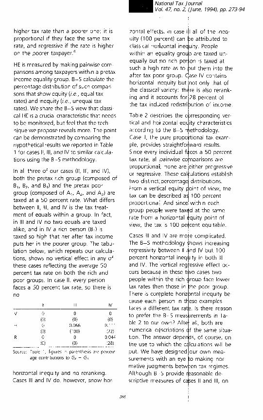
In all three of our cases (II, III, and IV), both the pretax rich group (composed of B,, Bz, and B3) and the pretax poor group (composed of A,, AI, and AJ are taxed at a 50 percent rate. What differs between II, III, and IV is the tax treatment of equals within a group. In fact, in III and IV no two equals are taxed alike, and in IV a rich person (B,) is taxed so high that her after tax income puts her in the poorer group. The tabu- lation below, which repeats our calcula-- tions, shows no vertical effect in any of these cases reflecting the average 50 percent tax rate on both the rich and poor groups. In case II, every person faces a 50 percent tax rate, so there is no

II III IV ----~-_

V (:I A:,

0 (0)

H 0 0 066 0.111 (0) (la.3 (72)

R k)

0.044

-&-..--- (281

Source: Table 1; figure<; In parenthem are percentage contnbutlons to Gx - GI,.

Ihorizontal inequity and no reranking. (Cases III and IV do,, however, show hon-

zontal effects. In case I/I all of the inequity (100 percent) can be attributed to classical norlizontal ineqluity. People withtn an equality grou~p are taxed un- equally but no rich per on

6

is taxed at such a high rate as to ut them into the after tax poor group. Case IV contains horizontal inequity but not only that of the classcal variety: there is also reranking and It accounts for~28 percent of the tax induced redistribution of inc:ome.

Table 2 describes the c rresponding vertical and horizontal eq

i ity characteristics

according to the B-S ~ ethodology. Case II, the pure proportional tax example, provides straightfodward results. Srnce every individual faces a 50 percent tax rate, all pairwise comparisons are proportional; none are either progressive or regressive. These calculations establish two distinct percentage distributions. From1 a vertrcal equity P oint of view, the tax can be described as 100 percent proportional. And since within each group peoplie were tax

1

d at the same rate from a horizontal quity point of view,. the tax is 100 percent equitable.

Cases III and IV are more complicated. The B-S methodology shows increasing regressivity between II and IV but 100 percent horizontal inequity in both III and IV. The vertical regressive effect oc- curs because in these two cases two people within the rich qroup face lower tax rates then those in the poor group. There is complete horiz

h”

ntal inequity because each person in t ese examples faces a different tax rat/e. Is there reason to prefer the B-S measurements in Ta- ble 2 to our own? Afte all, both are numerical descriptions

I f the same situa-

tion. The answer depends, of course, on the use tlo which the c

a

lculations WIII be put. We have designed our own measurements with an eye o making normative judgments betw

1

en tax regimes. Although B--S provide r asonable descriptive measures of calses II and III, on

288


TABLE 2 VERTICAL AND HORIZONTAL EQUITY CHARACTERISTICS OF AN INCOME TAX

(METHODOLOGY OF BERLIANT AND STRAUSS) [PERCENTAGE DISTRIBUTION]

Vertical Equity

II III IV

Progressive * 0 43 34 Proportional 100 8 6 Regressive

Horizontal equity Equity

0 49 100 60 100 - 100

100 0 0 Ineqiity 0 100 - 100

100 100 im

what basis can we choose between them? Case II is described as 100 percent proportional and 100 percent horizontally equitable; on the other hand, case III is 43 percent progressive and 100 percent horizontally inequitable.

There is no normative criterion on the basis of which to choose between these two regimes. The method of Table 1, however, which relies on the Gini coefficient, has a built-in implicit normative goal of aspiring to a more equal distribution of income. Thus, using our method of calculation, we can conclude that case II is superior to case III. In general, the advantage of the Gini coefficient approach is that it measures all forms of inequity on the same scale and thereby allows us to make a direct comparison of different sources of inequity.

That these measures have direct normative significance can be seen by comparing posttax welfare with that which would pertain after an equal-yield distri- butionally neutral tax, using Sen’s (1973) index; welfare is higher after intervening in the distribution by the amount

AW= ,w[G,- G,]=p.{V- H- R}

as before, where p is mean posttax income.7

Stephen Jenkins (1988c) focuses his at-

tention completely on horizontal equity and considers the problems that arise when the population is socially heterogeneous and the distributional effects we wish to consider are for the money (unequivalized) income distribution. For example, the group may at the same time include single people and married people. Jenkins clearly distinguishes between classical horizontal inequity and the inequity that arises when taxation changes people’s ranking in the income distribution. He adopts “a partial sym- metry” approach which he feels “lies between pure equal-treatment-of-equals and utility reranking and which is more readily empirically implementable.” See Jenkins (1988c, p. 306). To achieve his goal, he separates the population into homogeneous subgroups and creates a reranking index for each subgroup using an entropy index, which determines the gap between the distribution of actual posttax income and the distribution that would have existed if each person had maintained their pretax ranking. The technique offers a sophisticated (though disaggregated) measure of inequrty caused by reranking, but like B-S contains no normative rule. Moreover, it ap- plies only to the horizontal equity issue and not the vertical equity issue.

FIRST MEASUREMENTS OF V, H, AND R

Our first empincal estimates of V, H, and R are based on fiscal data reported in

the United Kingdom farnily expenditure survey (FES) as extensively analyzed in Aronson, Johnson, and Lambert (1994). We deflated a family’s money income (y)

by an equivalence scale factor (z), where z is of the form

In equatton (1 O), nA is the number of adults in the family and n, is the number of children. Thus, when 8 = 0, our equality groups are based on equal family income. For 8 ::> 0, economies of size

are assumed which decline as H is increased. Values of @ between 0 and 1 show the importance of children. When @ = 1, a child is made the equivalent of an adult and thus, the combination of 8 = 1 and at = 1 would mean that our

equality groups are based on equal per capita money Income. In short, equivalent income (utility) before tax, call this x, is

x = v. Z

We also converted each family’s tax payment and posttax income into equivalent income terms for the analysis. for the empirical analysis, we had first to identify the equals groups D(x), and this necessarily involved some roundrng or grouping of proximate x values com- puted as in equatiion 10. This is, of course, a vvell-recognized first step, ac. knowledged for example by Berliant and Strauss (1993, p. 16) in these words: “we take as given a partition of the economic income distribution Into cells of ‘equals.‘.” In Aronson, Johnson, and Lambert (1994) we grouped the x values first in f 5 per week ranges for ‘I 990--l, using the same real value for earlier

years, arid later testing the sensitivity results to the chosen b$ndwldth.

of

Table 3 reports the pretax and posttax Gini coelfrcrents and our estirnates of V, H, and R for 1!390-1 for the United King- dom for some sample vialues of @ and 8 (and with the bandwidth set at f5). Cal- cular;rons such as these must be consid- ered preliminary and tentative, but one striking result is that, over the entire range of values for @ and 8, V dominates H and R. This also held good as the f 5 bandwidth was reduced, although, un- surprisingly, H fell and Ip rose during this process. The paucity of exactly repeated A values In the FES sample (comprising around 10,000 family units) contributed to the decline in H (whiich became very small In the limiting case of a zero bandwidth), but this IS essentially a sarnpling problem, which should, In principle, be amenable to econometric methods; in the full population of 3D-milllon-plus United Kingdom family,units there have to ble plenty of repeats.8 Throughout the full rangle of values of + and ti explored, reranking R had two to three times the numerical implortance of pure horizontal InequIty H In the determination of redis- tnbutrve effect. For example, with @ = 8 = 0, the actual reduction in inequality ex- perienced, G, -- G, = 0.0269, is lower than that which could have been securecl had unequal treatment effects been ab- sent frorn the United Kingdom income tax in 1990-1, though not by very much (V =. 0.0290); pure horizontal inequity explained a “loss” of redistributive effect of some 1.7 percent, and reranking of about 5.5 percent. These relativities trans- late directly into the welfare importance of the tvvo phenomena, classical horizontal inequrty and reranking, through equa. tion 9.

Conclusions

Reranking has been proposed by some authors as (an alternative means to “get


TABLE 3 DECOMPOSITION OF CHANGE IN GINI COEFFICIENT, PRETAX AND POSTTAX 1990-1, UNITED KINGDOM

0 @ Gx GD Gx - CD v H R

0 0 0.4433 0.4164 0.0269 0.0290 0.4 0.4 0.4131 0.3828 0.0303 0.0322 1.0 1.0 0.4127 0.3816 0.03 11 0.0332

Source: FES, 1990-l. For further details, see Aronson, Johnson, and Lambert (1994).

0.0005 0.0016 0.0005 0.0015 0.0008 0.0013

a handle on” the inequity effects of an income tax to the strictly more correct business of detecting classical horizontal inequity. This is an appealing proposal, if only because of the sampling problem of identifying the “equals.” However, as our methodology and decomposition reveal, both phenomena contribute to the redistributive effect, and once a partition of the economic income distribution into cells of equals has been undertaken (rei- terating Berliant and Strauss’s words, 1993, p.l6), both may be consistently measured and taken into account.

Regarding the equals problem, Berliant and Strauss (1993) follow their remark by a claim that “the empirical ordering of tax systems is generally independent of these partitions . . .” This proposition has not (yet) been fully tested in respect of our measures H and R, and is one area for future research, which our methodology opens up. In particular, mi- nor changes in partition clearly may cast taxpayers with closely adjacent incomes into different equality groups; does this necessarily have only minor effects upon H and R? The results in Aronson, John- son, and Lambert (1994) are encourag- ing, but not conclusive. Statistical issues of estimation from small samples and the associated confidence limits are also raised by our measurement methodology. Nevertheless, our approach can be used both to gauge the equity effects of tax reforms and for purposes of international comparison.

Other measurement methodologies are

291

of course also subject to caveats. These include the approach of Berliant and Strauss (1993) for the measurement of classical horizontal inequity, and of Jen- kins (1988~) for the measurement of reranking. In our own case, the welfare link exposed in equation 9 gives normative significance to all effects at once- the vertical, the horizontal, and the reranking-and this is necessarily lacking in partial approaches.

In assessing tax reform, the reranking term R captures an effect which is seen as equity-relevant by Atkinson (1980) and Plotnick (1981) as well as by our- selves. The reranking effect becomes normatively significant precisely because we chose to use the Gini to measure inequality, rather than, say, opting to use a decomposable (generalized entropy) index. In practical terms, had we followed the latter route, the residual term R would not have appeared in equation 1, and reranking would thus have been ab- sent from decomposition 2, leaving only vertical and pure horizontal effects in terms of which to assess tax reforms. Normatively, the significance or insignifi- cance of reranking hinges upon whether we opt to capture in our measures the unfairness of inequality, which rank changes bear upon (and which the Gini measures), or rather the wastefulness of inequality, for which the ranks people occupy typically do not matter. Broome (1989) discusses this distinction; in pre- senting our methodology, we would ar- gue for the former course.’

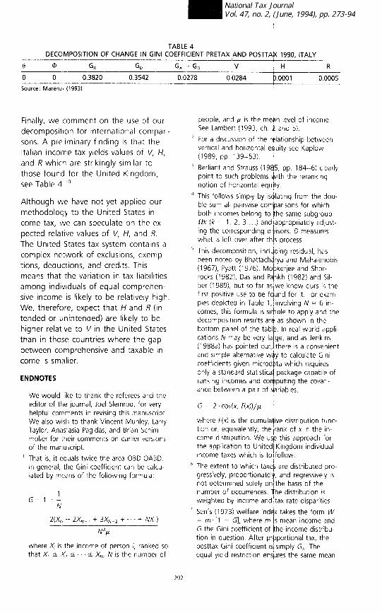
TABLE 4 DECOMPOSITION OF CHANGE IN GINI COEFFICIENT PRETAX AND POSlTAX 1990. ITALY

0 ct, Gx GI, Gx GD v H R

0 0 0.3820 0.3542 0.0278 0.0284 0.000 1 0.0005

Source: Marem (1993).

Finally, we comment on the use of our decomposiiion for international comparisons. A preliminary finding is that the Italian income tax yields values of V, H, and R which are strikingly similar to those found for the United Kingdom; see Table 4.”

Although we have not yet applied our methodology to the United States income tax, we can speculate on the ex- pected relative values of V, H, and R. The United States tax system contains C~ complex network of exclusions, exemp- tions, deductions, and credits. This means that the variation in tax liabilities among individuals of equal comprehen.. sive income is likely to be relatively high. We, therefore, expect that H and R (in- tended or unintended) are likely to be higher relative to I/ in the United States than in those countries where the gap between comprehensive and taxable income is smaller.

ENDNOTES

We would like to thank the referees and the editor of the Journal, Joel Slemrod, for very helpful comments in revising this manuscript. We also wish to th,jnk Vincent Munley, Larry Taylor, Anastasia Pagidas, and Brian Schlm- moller for their comments on earlier versions of the manuscript.

’ That is, it equals twice the area OBD-OABD. In general, the Gini coefficient can be calculated by means of Ihe followlng formula.

G=,+l N

2(Xf, -t 2X,- + 3XN.* +. . i NX,) - ---------

N .'p

where X, is the Income of person i, ranked so that X, 5 ,X2 5;. . . 12 X,!, N IS the number of

people, and Al. is the mean level of Income See Larnbert (1993, ch. 2 and 5)

For a dIscussion of the relatIonship between vertical anti horizontal equity see Kaplow (1’389, pp. 13!3-53).

Berllant and Strauss (1985, pp. 184 -6) clearlp point to such problems &tth the reranking notion of horizontal equity.

This follows simply by lsolatlng from the dou- ble sum all paIrwIse comlpansons for which both In:omes belong to the sarne subgroup 111: (k q = 1, 2, 3 .) and appropriately adjust- ing the corresponding ditiisors. D measures what is left over after this process.

This decomposition, rnclqding residual, has been noted by Bhattachdrya and Mahalanobls (1967), Pyatt (1976), Mobkerjee and Shor- rocks (19821, Das and Palrikh (1982) and Sd- ber (1989), but so far as we know ours IS the first posltlve use to be faund for it IFor examples deplcttrd in Table 1,‘lnvolving N = 6 tn- comes, thts formula is slrhple to apply and the decomposition results are as shown in the bottom panel of the tablp. In real-world appll. cations N may be very lalge, and as Jenkins (1988a) has pointed out,’ there IS a convenieni and slrrple alternative w4y to calculate Gin colefflclents given mlcrod+ta which requires only a standard statistical package capable of ranking Incomes and cot$putlng the covarl- ante between a pair of variables,

G =z 2. cov(x, F(x))/p

where f-(x) IS the cumularllve dlstnbutlon function or, equivalently, the irank of x in the in- col-ne d stnbution. We usle this approach for the appllcatlon to United1 Klngdorn individual Income taxes which is to~follow

Thlz extent to which taxeb are distributed pro- gresslvely, proportionately, and regressively IS not determined solely on the basis of the number of occurrences. l/he distribution IS

weighted by Income and’tax rate disparities.

Sen’s (1973) welfare inddx takes the form W = rn. [l - G], where m 1s mean income and G the Cltnl coefficient of hhe Income distrtbu- tlon in que>tton. After prpportional tax, the posttax GinI coefficient is simply Gx. The equal-yilzld restriction ensures the sarne mean


posttax income. For more on this welfare index, see Lambert (1993, ch. 5).

a Our model helps articulate the implications of this sampling problem. If there were no repeated x-values in a given sample, and no grouping of proximate x-values were undertaken, then each tax payment would be associated with a unique income level and noth- ing could be learned about classical horizontal inequity from the data set.

’ As an example of the perceived relevance of reranking, consider a reform of the tax system shown as scenario Ill in Table 1, in which person A3 in the higher equality group gains $50 (going from $550 to $600) and person B, loses $50 (going from $600 to $550). Noth- ing has happened to the overall distribution of posttax income as a result of this rich-to- poor income transfer, and so welfare is un- changed by any measure. An entropy approach would explain this in terms of exactly balancing vertical and horizontal effects, but crucially it is the violation of the rank- preserving caveat in the principle of transfers, which explains the zero welfare impact. Our measures pick this up: calling the new scenario Ill*, one may calculate v* = +0.012, H* = +0.073, and R* = +.005, and compare with V = 0, H = 0.066, and R = 0 for scenario III. The change has, to be sure, improved vertical equity (by 12 points) and exac- erbated horizontal inequity (by seven points), but it has also introduced five points worth of reranking, and it is this which is the balancing item.

lo See Marenzi (1993).

REFERENCES

Aronson, J. Richard, Paul Johnson, and Peter 1. Lambert. “Redistributive Effect and Unequal Income Tax Treatment.” The Economic /ourna/ 104, forthcoming (1994).

Atkinson, Anthony B. “Horizontal Equity and the Distribution of the Tax Burden.” In The Eco- nomics of Taxation, edited by H. Aaron and M. Boskin. Washington, D.C.: The Brookings Institu- tion, 1980. Berglas, Etan. “Income Tax and the Distribution of Income: An International Comparison.” Public Finance/Finances Publiques 26 (1971): 532-45. Berliant, Marcus C. and Robert P. Strauss. “The Horizontal and Vertical Equity Characteris- tics of the Federal Individual Income Tax, 1966- 77.” In National Bureau of Economic Research, Studies in income and Wealth, edited by M. David and T. Smeeding, Chicago: University of Chicago Press, 1985, vol. 50, 179-214.

Berliant, Marcus C. and Robert P. Strauss. “State and Federal Tax Equity: Estimates Before and After the Tax Reform Act of 1986.” Journal of Poky Analysis and Management 12 (No. 1, 1993): 9-43. Bhattacharya, N. and B. Mahalanobis. “Re- gional Disparities in Household Consumption in India.” Journal of the American Statistical Associ- ation 62 (1967): 143-61. Broome, John. “What’s the Good of Equality?” In Current issues in Microeconomics, edited by 1. D. Hey, ch. 9. London: Macmillan, 1989. Das, T. and Ashok Parikh. “Decomposition of Inequality Measures and a Comparative Analy- sis.” Empirical Economics 7 (1982): 23-48. Feldstein, Martin. “Compensation in Tax Re- form.” National Tax Journal 29 (No. 2, 1976): 123-30. Jenkins, Stephen. “‘Calculating Income Distribu- tion Indices from Micro Data.” National Tax Jour- nal 41, (1988a): 139-42. Jenkins, Stephen. “Reranking and the Analysis of Income Redistribution.” Scottish Journal of Po- litical Economy 35, (1988b): 65-76. Jenkins, Stephen. “Empirical Measurement of Horizontal Inequtty.” Journal of Public Economics 37 (1988c): 305-29. Johnson, Shirley B. and Thomas Mayer. “An Extension of Sidgwick’s Equity Principle.” Quar- terly Journal of Economics 76 (1962): 454-63. Kakwani, Nanak C. “On the Measurement of Tax Progressivity and Redistributive Effect of Taxes with Applications to Horizontal and Verti- cal Equity.” Advances in Econometrics 3, (1984): 149-68. Kaplow, Louis. “Horizontal Equity: Measures in Search of a Principle.” National Tax Journal (1989): 739-53. Lambett, Peter. J. The D&rib&ion and Redisrri- bution of Income. A Mathematical Analysis. 2nd ed. Manchester: University Press, 1993. Lambert, Peter 1. and 1. Richard Aronson. “Inequality Decomposition Analysis and the Gini Coefficient Revisited.” The Economic Journal 103, (1993): 1221-7.

Marenzi, Anna. 1993. Equita’ Verticale, Oriz- zontale ed Effetto di Riordinamento: Una Stima per I’ltalia. University of York. Mimeo. Mookerjee, Dilip and Anthony F. Sharrocks. “A Decomposition Analysis of the Trend in U.K. Income Inequality.” Economic Journal 92 (1992): 886-902. Musgrave, Richard A. The Theory of Public Fi- nance. New York: McGraw-Hill, 1959. Musgrave, Richard A. “Horizontal Equity, Once More.” National Tax Journal 43 (No. 2, 1990): 113-22.

2.93

Pechman, Joseph A. and Benjamin A. Okner. Who Bears the Tax Burden? Washington, D.C.:

The Brookings Institution, 1974.

Pigou, A. C. Public Finance London: Macmillan, 1960. Plotnick, Robert. “A Measure of Horizontal In equity.” Review of Economics and 5tatisks 63 (1981): 283-8. Plotnick, Robert. “A Comparison of Measures of Horizontal Inequity.” In Horizontal Equity, Un- certainty and Economic Well-Being, edited by M. David and T. !<meeding, ch 8. New York NBER, 1985.

Pyatt, Graham. “The Interpretation and Disag- gregatlon of Gini Coefficien{s.” Economic J’our- nal 8 (1976): 243-55.

of Income. The United Statqs, 1950, 1967, 1970. New York: Academic ~Press, 1977.

Sen, Amartya. On Economdc Clarendon Press, 1973.

Inequality Oxford :

Silber, Jacques. “Factor Copponents, Popula- tion Subgroups and the Cor$putation of the Gini Index of Inequality.” Review of Economics and Statist/es 77 (1989): 107-l 5.

Documents

DECOMPOSING THE GIN1 COEFFICIENT TO REVEAL … · DECOMPOSING THE GIN1 COEFFICIENT TO REVEAL THE VERTICAL, HORIZONTAL, AND RERANKING EFFECTS OF INCOME TAXATION 1. RICHARD ... income