Embed Size (px)
Citation preview
121121
4chapter
Decoupling the train? SpilloverS anD cycleS in the global economy
Over the past year, there has been considerable debate about how the slowing of the U.S. economy could affect other countries. The concerns
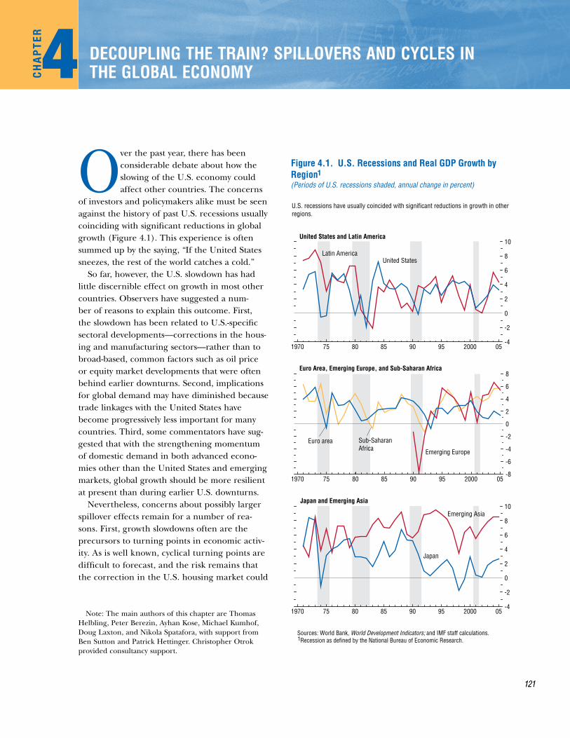
of investors and policymakers alike must be seen against the history of past U.S. recessions usually coinciding with significant reductions in global growth (Figure 4.1). This experience is often summed up by the saying, “If the United States sneezes, the rest of the world catches a cold.”
So far, however, the U.S. slowdown has had little discernible effect on growth in most other countries. Observers have suggested a num-ber of reasons to explain this outcome. First, the slowdown has been related to U.S.-specific sectoral developments—corrections in the hous-ing and manufacturing sectors—rather than to broad-based, common factors such as oil price or equity market developments that were often behind earlier downturns. Second, implications for global demand may have diminished because trade linkages with the United States have become progressively less important for many countries. Third, some commentators have sug-gested that with the strengthening momentum of domestic demand in both advanced econo-mies other than the United States and emerging markets, global growth should be more resilient at present than during earlier U.S. downturns.
Nevertheless, concerns about possibly larger spillover effects remain for a number of rea-sons. First, growth slowdowns often are the precursors to turning points in economic activ-ity. As is well known, cyclical turning points are difficult to forecast, and the risk remains that the correction in the U.S. housing market could
Note: The main authors of this chapter are Thomas Helbling, Peter Berezin, Ayhan Kose, Michael Kumhof, Doug Laxton, and Nikola Spatafora, with support from Ben Sutton and Patrick Hettinger. Christopher Otrok provided consultancy support.
1970 75 80 85 90 95 2000 05-4
-2
0
2
4
6
8
10
1970 75 80 85 90 95 2000 05-8
-6
-4
-2
0
2
4
6
8
1970 75 80 85 90 95 2000 05-4
-2
0
2
4
6
8
10
Figure 4.1. U.S. Recessions and Real GDP Growth by Region(Periods of U.S. recessions shaded, annual change in percent)
U.S. recessions have usually coincided with significant reductions in growth in other regions.
Sources: World Bank, World Development Indicators; and IMF staff calculations. Recession as defined by the National Bureau of Economic Research.
United States and Latin America
1
1
Euro Area, Emerging Europe, and Sub-Saharan Africa
Japan and Emerging Asia
Latin AmericaUnited States
Euro area
Emerging Europe
Sub-SaharanAfrica
Japan
Emerging Asia
chapter 4 Decoupling the train? SpilloverS anD cycleS in the global economy
122
be deeper than expected and the current U.S. slowdown could intensify, with likely larger spill-overs into other countries.1 Second, the rela-tive decline in trade linkages with the United States must be balanced against the rapidly increasing cross-border financial linkages and the fact that the United States remains at the core of the global financial system. Third, the U.S. economy remains the world’s largest, and while other advanced economies, in particular in Europe, have gained cyclical momentum, there remain questions about their underlying dynamism. Fourth, while the five largest emerg-ing market economies now account for one-fourth of global GDP on a purchasing power parity (PPP) basis, their role in global trade is not yet commensurate (about one-seventh), and it is difficult to argue that they could entirely replace the U.S. economy as an engine for global growth.
Against this background, the chapter asks the broad question of how far other countries can “decouple” from the U.S. economy and sustain strong growth in the face of a U.S. slowdown. The main goal is to (1) pinpoint what factors would likely determine the magnitude of the spillovers—the effects on the output of other countries from weaker U.S. growth—in present
1See, among others, Artis (1996) and Timmermann (2006) on forecasting turning points.
circumstances; and (2) provide an understand-ing of the risks and policy challenges that apply not just at this conjuncture but also to future cycles.
The chapter has two main parts. The first part analyzes recent evidence on how the U.S. economy has affected (and been affected by) international business cycle fluctuations. Specifi-cally, it addresses the following questions.• What have been the global repercussions of
past U.S. recessions and slowdowns, and how have these repercussions changed over time?
• How much do disturbances in the United States affect macroeconomic conditions elsewhere, and how do these effects compare with those from disturbances in other major currency areas? Has the strength of these busi-ness cycle linkages changed over time with the rapid increases in international trade and financial integration?
• How much have synchronized cycles in eco-nomic activity across the major economies been driven by common factors?The second part of the chapter uses a model-
based simulation approach to analyze how the global repercussions of a U.S. slowdown depend on the specific underlying disturbances. This section also considers the role that monetary and exchange rate policies could play in reduc-ing the extent of adverse spillovers from a U.S. slowdown.
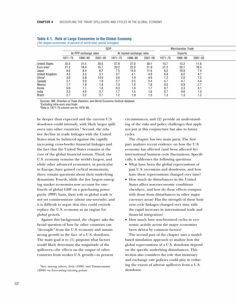
table 4.1. role of large economies in the global economy(Ten largest economies, in percent of world total; period averages)
GDP Merchandise Trade Merchandise Trade _____________________________________________________________ ________________________________________________________________________________________________ At PPP exchange rates At market exchange rates Exports Imports Stock Market Capitalization _____________________________ ____________________________ _____________________________ _________________________ _________________________ 1971–75 1986–90 2001–05 1971–75 1986–90 2001–05 1971–75 1986–90 2001–05 1971–75 1986–90 2001–05 1971–75 1986–90 2001–05
United States 22.5 21.5 20.5 27.9 27.0 30.1 15.7 13.2 11.6 15.6 18.6 19.7 . . . 32.8 44.4Euro area1 21.3 18.4 15.7 20.2 22.0 21.9 21.2 20.1 18.5 21.2 19.0 16.9 . . . 11.3 15.3Japan 8.0 8.4 6.7 7.5 14.0 11.6 8.5 10.9 7.4 7.9 7.4 5.8 . . . 34.4 9.4United Kingdom 4.3 3.5 3.1 3.7 4.1 4.9 6.9 6.2 4.7 7.9 7.3 5.6 . . . 7.9 7.5China2 3.0 5.8 14.0 2.6 1.9 4.6 1.2 2.0 7.2 1.3 2.1 6.2 . . . . . . 1.9Canada 2.1 2.0 1.9 2.7 2.5 2.4 5.7 4.7 4.4 5.5 4.7 4.0 . . . 2.6 2.8Mexico 1.7 1.9 1.8 1.3 1.0 1.8 0.5 0.9 2.7 0.8 0.9 2.9 . . . 0.2 0.5Korea 0.6 1.1 1.6 0.3 1.0 1.7 0.7 2.3 3.1 0.9 2.1 2.7 . . . 0.8 1.1India 3.5 4.0 5.7 1.7 1.5 1.6 0.7 0.6 1.0 0.8 0.8 1.2 . . . 0.3 0.8Brazil 2.7 3.2 2.7 1.2 1.9 1.5 1.3 1.3 1.2 1.9 0.8 0.9 . . . 0.3 0.8
Sources: IMF, Direction of Trade Statistics, and World Economic Outlook database. 1Excluding intra–euro area trade.2Data in 1971–75 column are for 1976–80.
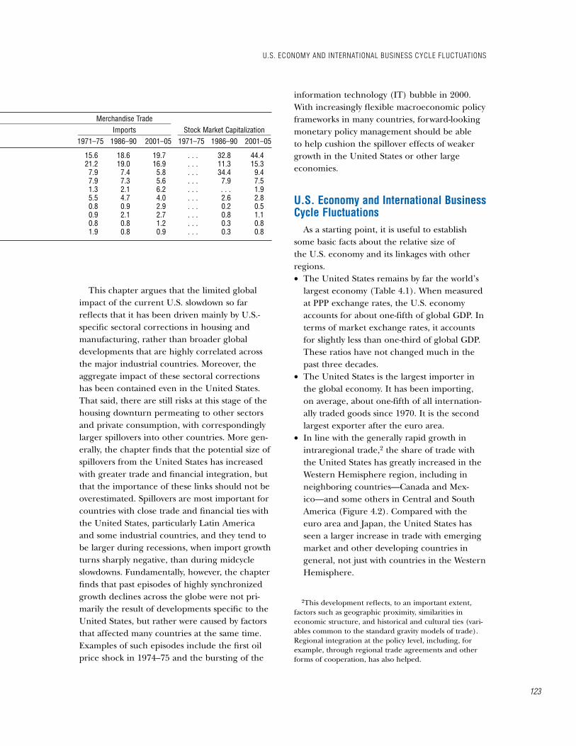
This chapter argues that the limited global impact of the current U.S. slowdown so far reflects that it has been driven mainly by U.S.-specific sectoral corrections in housing and manufacturing, rather than broader global developments that are highly correlated across the major industrial countries. Moreover, the aggregate impact of these sectoral corrections has been contained even in the United States. That said, there are still risks at this stage of the housing downturn permeating to other sectors and private consumption, with correspondingly larger spillovers into other countries. More gen-erally, the chapter finds that the potential size of spillovers from the United States has increased with greater trade and financial integration, but that the importance of these links should not be overestimated. Spillovers are most important for countries with close trade and financial ties with the United States, particularly Latin America and some industrial countries, and they tend to be larger during recessions, when import growth turns sharply negative, than during midcycle slowdowns. Fundamentally, however, the chapter finds that past episodes of highly synchronized growth declines across the globe were not pri-marily the result of developments specific to the United States, but rather were caused by factors that affected many countries at the same time. Examples of such episodes include the first oil price shock in 1974–75 and the bursting of the
information technology (IT) bubble in 2000. With increasingly flexible macroeconomic policy frameworks in many countries, forward-looking monetary policy management should be able to help cushion the spillover effects of weaker growth in the United States or other large economies.
u.S. economy and international business cycle Fluctuations
As a starting point, it is useful to establish some basic facts about the relative size of the U.S. economy and its linkages with other regions.• The United States remains by far the world’s
largest economy (Table 4.1). When measured at PPP exchange rates, the U.S. economy accounts for about one-fifth of global GDP. In terms of market exchange rates, it accounts for slightly less than one-third of global GDP. These ratios have not changed much in the past three decades.
• The United States is the largest importer in the global economy. It has been importing, on average, about one-fifth of all internation-ally traded goods since 1970. It is the second largest exporter after the euro area.
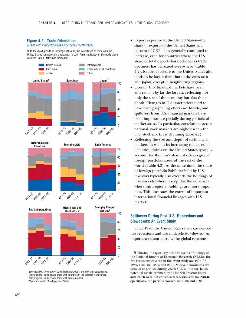
• In line with the generally rapid growth in intraregional trade,2 the share of trade with the United States has greatly increased in the Western Hemisphere region, including in neighboring countries—Canada and Mex-ico—and some others in Central and South America (Figure 4.2). Compared with the euro area and Japan, the United States has seen a larger increase in trade with emerging market and other developing countries in general, not just with countries in the Western Hemisphere.
2This development reflects, to an important extent, factors such as geographic proximity, similarities in economic structure, and historical and cultural ties (vari-ables common to the standard gravity models of trade). Regional integration at the policy level, including, for example, through regional trade agreements and other forms of cooperation, has also helped.
u.S. economy anD international buSineSS cycle FluctuationS
123
table 4.1. role of large economies in the global economy(Ten largest economies, in percent of world total; period averages)
GDP Merchandise Trade Merchandise Trade _____________________________________________________________ ________________________________________________________________________________________________ At PPP exchange rates At market exchange rates Exports Imports Stock Market Capitalization _____________________________ ____________________________ _____________________________ _________________________ _________________________ 1971–75 1986–90 2001–05 1971–75 1986–90 2001–05 1971–75 1986–90 2001–05 1971–75 1986–90 2001–05 1971–75 1986–90 2001–05
United States 22.5 21.5 20.5 27.9 27.0 30.1 15.7 13.2 11.6 15.6 18.6 19.7 . . . 32.8 44.4Euro area1 21.3 18.4 15.7 20.2 22.0 21.9 21.2 20.1 18.5 21.2 19.0 16.9 . . . 11.3 15.3Japan 8.0 8.4 6.7 7.5 14.0 11.6 8.5 10.9 7.4 7.9 7.4 5.8 . . . 34.4 9.4United Kingdom 4.3 3.5 3.1 3.7 4.1 4.9 6.9 6.2 4.7 7.9 7.3 5.6 . . . 7.9 7.5China2 3.0 5.8 14.0 2.6 1.9 4.6 1.2 2.0 7.2 1.3 2.1 6.2 . . . . . . 1.9Canada 2.1 2.0 1.9 2.7 2.5 2.4 5.7 4.7 4.4 5.5 4.7 4.0 . . . 2.6 2.8Mexico 1.7 1.9 1.8 1.3 1.0 1.8 0.5 0.9 2.7 0.8 0.9 2.9 . . . 0.2 0.5Korea 0.6 1.1 1.6 0.3 1.0 1.7 0.7 2.3 3.1 0.9 2.1 2.7 . . . 0.8 1.1India 3.5 4.0 5.7 1.7 1.5 1.6 0.7 0.6 1.0 0.8 0.8 1.2 . . . 0.3 0.8Brazil 2.7 3.2 2.7 1.2 1.9 1.5 1.3 1.3 1.2 1.9 0.8 0.9 . . . 0.3 0.8
Sources: IMF, Direction of Trade Statistics, and World Economic Outlook database. 1Excluding intra–euro area trade.2Data in 1971–75 column are for 1976–80.
chapter 4 Decoupling the train? SpilloverS anD cycleS in the global economy
124
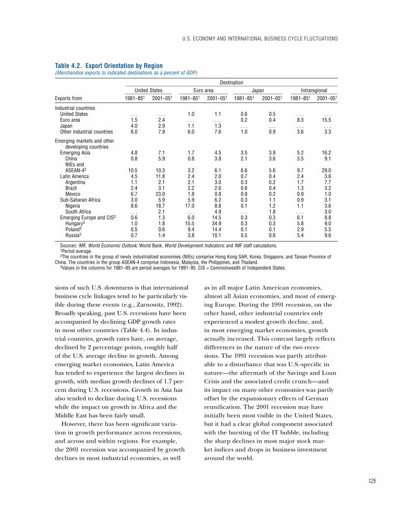
• Export exposure to the United States—the share of exports to the United States as a percent of GDP—has generally continued to increase, even for countries where the U.S. share of total exports has declined, as trade openness has increased everywhere (Table 4.2). Export exposure to the United States also tends to be larger than that to the euro area and Japan, except in neighboring regions.
• Overall, U.S. financial markets have been and remain by far the largest, reflecting not only the size of the economy but also their depth. Changes in U.S. asset prices tend to have strong signaling effects worldwide, and spillovers from U.S. financial markets have been important, especially during periods of market stress. In particular, correlations across national stock markets are highest when the U.S. stock market is declining (Box 4.1).
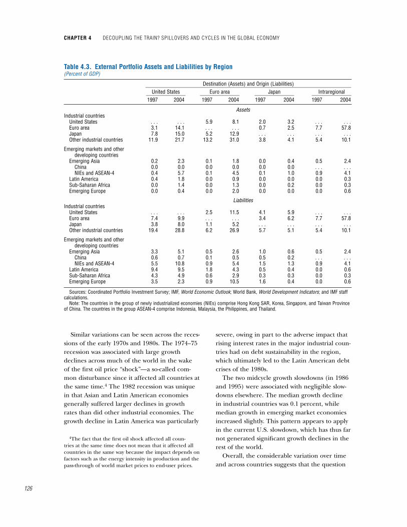
• Reflecting the size and depth of its financial markets, as well as its increasing net external liabilities, claims on the United States typically account for the lion’s share of extra-regional foreign portfolio assets of the rest of the world (Table 4.3). At the same time, the share of foreign portfolio liabilities held by U.S. investors typically also exceeds the holdings of investors elsewhere, except for the euro area, where intraregional holdings are more impor-tant. This illustrates the extent of important international financial linkages with U.S. markets.
Spillovers During past u.S. recessions and Slowdowns: an event Study
Since 1970, the United States has experienced five recessions and two midcycle slowdowns.3 An important reason to study the global repercus-
3Following the quarterly business cycle chronology of the National Bureau of Economic Research (NBER), the five recessions covered in the event study are 1974–75, 1980, 1981–82, 1991, and 2001. Midcycle slowdowns are defined as periods during which U.S. output was below potential (as determined by a Hodrick-Prescott filter) and which were not considered recessions by the NBER. Specifically, the periods covered are 1986 and 1995.
Figure 4.2. Trade Orientation(Trade with indicated areas as percent of total trade)
With the rapid growth in intraregional trade, the importance of trade with the United States has generally decreased. In Latin America, however, the trade share with the United States has increased.
Sources: IMF, Direction of Trade Statistics (2006); and IMF staff calculations. Intraregional trade covers trade with countries in the Western Hemisphere. Intraregional trade covers trade with emerging Asia. Commonwealth of Independent States.
40
20
60
80
100
United States
United States Euro Area Japan
1971
–75
1986
–90
2001
–05
1971
–75
1986
–90
2001
–05
1971
–75
1986
–90
2001
–05
Euro areaJapan
IntraregionalOther industrial countriesOther
Other Industrial Countries
1971
–75
1986
–90
2001
–05
1971
–75
1986
–90
2001
–05
1971
–75
1986
–90
2001
–05
Emerging Asia Latin America
Sub-Saharan Africa
1971
–75
1986
–90
2001
–05
1971
–75
1986
–90
2001
–05
1991
–95
2001
–05
Middle East and North Africa
Emerging Europe and CIS
1 2
12
0
40
20
60
80
100
0
40
20
60
80
100
0
3
3
sions of such U.S. downturns is that international business cycle linkages tend to be particularly vis-ible during these events (e.g., Zarnowitz, 1992). Broadly speaking, past U.S. recessions have been accompanied by declining GDP growth rates in most other countries (Table 4.4). In indus-trial countries, growth rates have, on average, declined by 2 percentage points, roughly half of the U.S. average decline in growth. Among emerging market economies, Latin America has tended to experience the largest declines in growth, with median growth declines of 1.7 per-cent during U.S. recessions. Growth in Asia has also tended to decline during U.S. recessions while the impact on growth in Africa and the Middle East has been fairly small.
However, there has been significant varia-tion in growth performance across recessions, and across and within regions. For example, the 2001 recession was accompanied by growth declines in most industrial economies, as well
as in all major Latin American economies, almost all Asian economies, and most of emerg-ing Europe. During the 1991 recession, on the other hand, other industrial countries only experienced a modest growth decline, and, in most emerging market economies, growth actually increased. This contrast largely reflects differences in the nature of the two reces-sions. The 1991 recession was partly attribut-able to a disturbance that was U.S.-specific in nature—the aftermath of the Savings and Loan Crisis and the associated credit crunch—and its impact on many other economies was partly offset by the expansionary effects of German reunification. The 2001 recession may have initially been most visible in the United States, but it had a clear global component associated with the bursting of the IT bubble, including the sharp declines in most major stock mar-ket indices and drops in business investment around the world.
table 4.2. export orientation by region(Merchandise exports to indicated destinations as a percent of GDP)
Destination __________________________________________________________________________________ United States Euro area Japan Intraregional __________________ ___________________ ___________________ __________________Exports from 1981–851 2001–051 1981–851 2001–051 1981–851 2001–051 1981–851 2001–051
Industrial countriesUnited States . . . . . . 1.0 1.1 0.6 0.5 . . . . . .Euro area 1.5 2.4 . . . . . . 0.2 0.4 8.3 15.5Japan 4.0 2.9 1.1 1.3 . . . . . . . . . . . .Other industrial countries 6.0 7.9 6.0 7.6 1.0 0.9 3.6 3.3
Emerging markets and other developing countries
Emerging Asia 4.8 7.1 1.7 4.5 3.5 3.9 5.2 16.2China 0.8 5.9 0.8 3.8 2.1 3.6 3.5 9.1NIEs andASEAN-42 10.5 10.3 3.2 6.1 6.6 5.6 9.7 29.0
Latin America 4.5 11.8 2.4 2.0 0.7 0.4 2.4 3.6Argentina 1.1 2.1 2.1 3.0 0.3 0.2 1.7 7.7Brazil 2.4 3.1 2.2 2.6 0.6 0.4 1.3 3.2Mexico 6.7 23.0 1.8 0.8 0.8 0.2 0.9 1.0
Sub-Saharan Africa 3.0 5.9 5.9 6.2 0.3 1.1 0.9 3.1Nigeria 8.6 18.7 17.0 8.8 0.1 1.2 1.1 3.6South Africa . . . 2.1 . . . 4.9 . . . 1.8 . . . 3.0
Emerging Europe and CIS3 0.6 1.3 6.0 14.5 0.3 0.3 6.1 8.8Hungary3 1.0 1.8 15.5 34.9 0.3 0.3 5.8 9.0Poland3 0.5 0.6 9.4 14.4 0.1 0.1 2.9 5.5Russia3 0.7 1.4 3.8 10.1 0.5 0.6 5.4 9.6
Sources: IMF, World Economic Outlook; World Bank, World Development Indicators; and IMF staff calculations.1Period average.2The countries in the group of newly industrialized economies (NIEs) comprise Hong Kong SAR, Korea, Singapore, and Taiwan Province of
China. The countries in the group ASEAN-4 comprise Indonesia, Malaysia, the Philippines, and Thailand.3Values in the columns for 1981–85 are period averages for 1991–95. CIS = Commonwealth of Independent States.
u.S. economy anD international buSineSS cycle FluctuationS
125
chapter 4 Decoupling the train? SpilloverS anD cycleS in the global economy
126
Similar variations can be seen across the reces-sions of the early 1970s and 1980s. The 1974–75 recession was associated with large growth declines across much of the world in the wake of the first oil price “shock”—a so-called com-mon disturbance since it affected all countries at the same time.4 The 1982 recession was unique in that Asian and Latin American economies generally suffered larger declines in growth rates than did other industrial economies. The growth decline in Latin America was particularly
4The fact that the first oil shock affected all coun-tries at the same time does not mean that it affected all countries in the same way because the impact depends on factors such as the energy intensity in production and the pass-through of world market prices to end-user prices.
severe, owing in part to the adverse impact that rising interest rates in the major industrial coun-tries had on debt sustainability in the region, which ultimately led to the Latin American debt crises of the 1980s.
The two midcycle growth slowdowns (in 1986 and 1995) were associated with negligible slow-downs elsewhere. The median growth decline in industrial countries was 0.1 percent, while median growth in emerging market economies increased slightly. This pattern appears to apply in the current U.S. slowdown, which has thus far not generated significant growth declines in the rest of the world.
Overall, the considerable variation over time and across countries suggests that the question
table 4.3. external portfolio assets and liabilities by region(Percent of GDP)
Destination (Assets) and Origin (Liabilities) ______________________________________________________________________________ United States Euro area Japan Intraregional _______________ _______________ _______________ _______________ 1997 2004 1997 2004 1997 2004 1997 2004
AssetsIndustrial countries
United States . . . . . . 5.9 8.1 2.0 3.2 . . . . . .Euro area 3.1 14.1 . . . . . . 0.7 2.5 7.7 57.8Japan 7.8 15.0 5.2 12.9 . . . . . . . . . . . .Other industrial countries 11.9 21.7 13.2 31.0 3.8 4.1 5.4 10.1
Emerging markets and other developing countries
Emerging Asia 0.2 2.3 0.1 1.8 0.0 0.4 0.5 2.4China 0.0 0.0 0.0 0.0 0.0 0.0 . . . . . .NIEs and ASEAN-4 0.4 5.7 0.1 4.5 0.1 1.0 0.9 4.1
Latin America 0.4 1.8 0.0 0.9 0.0 0.0 0.0 0.3Sub-Saharan Africa 0.0 1.4 0.0 1.3 0.0 0.2 0.0 0.3Emerging Europe 0.0 0.4 0.0 2.0 0.0 0.0 0.0 0.6
LiabilitiesIndustrial countries
United States . . . . . . 2.5 11.5 4.1 5.9 . . . . . .Euro area 7.4 9.9 . . . . . . 3.4 6.2 7.7 57.8Japan 3.8 8.0 1.1 5.2 . . . . . . . . . . . .Other industrial countries 19.4 28.8 6.2 26.9 5.7 5.1 5.4 10.1
Emerging markets and other developing countries
Emerging Asia 3.3 5.1 0.5 2.6 1.0 0.6 0.5 2.4China 0.6 0.7 0.1 0.5 0.5 0.2 . . . . . .NIEs and ASEAN-4 5.5 10.8 0.9 5.4 1.5 1.3 0.9 4.1
Latin America 9.4 9.5 1.8 4.3 0.5 0.4 0.0 0.6Sub-Saharan Africa 4.3 4.9 0.6 2.9 0.3 0.3 0.0 0.3Emerging Europe 3.5 2.3 0.9 10.5 1.6 0.4 0.0 0.6
Sources: Coordinated Portfolio Investment Survey; IMF, World Economic Outlook; World Bank, World Development Indicators; and IMF staff calculations.
Note: The countries in the group of newly industrialized economies (NIEs) comprise Hong Kong SAR, Korea, Singapore, and Taiwan Province of China. The countries in the group ASEAN-4 comprise Indonesia, Malaysia, the Philippines, and Thailand.
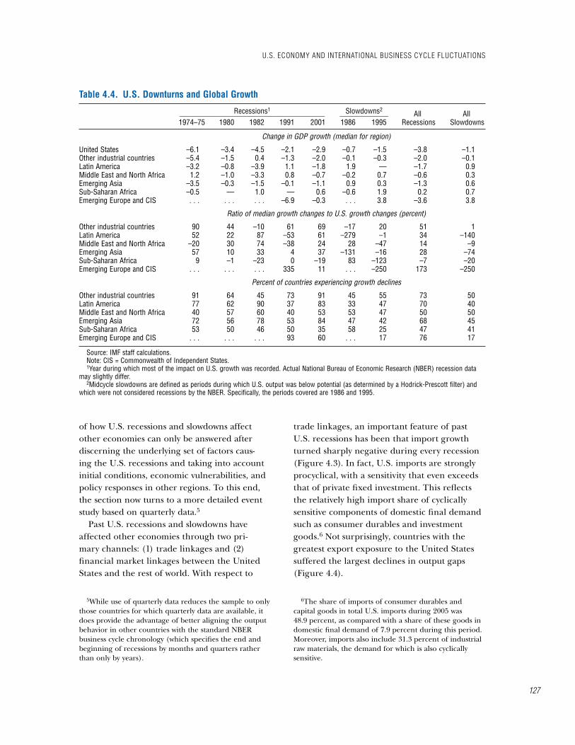
of how U.S. recessions and slowdowns affect other economies can only be answered after discerning the underlying set of factors caus-ing the U.S. recessions and taking into account initial conditions, economic vulnerabilities, and policy responses in other regions. To this end, the section now turns to a more detailed event study based on quarterly data.5
Past U.S. recessions and slowdowns have affected other economies through two pri-mary channels: (1) trade linkages and (2) financial market linkages between the United States and the rest of world. With respect to
5While use of quarterly data reduces the sample to only those countries for which quarterly data are available, it does provide the advantage of better aligning the output behavior in other countries with the standard NBER business cycle chronology (which specifies the end and beginning of recessions by months and quarters rather than only by years).
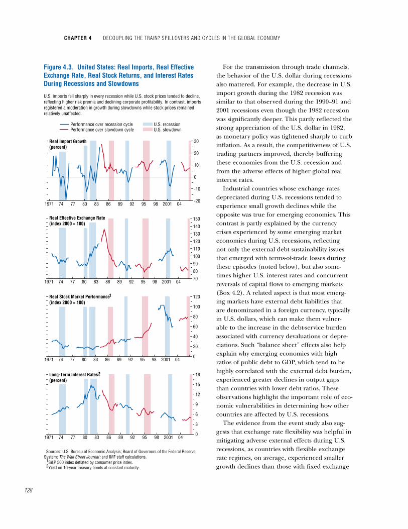
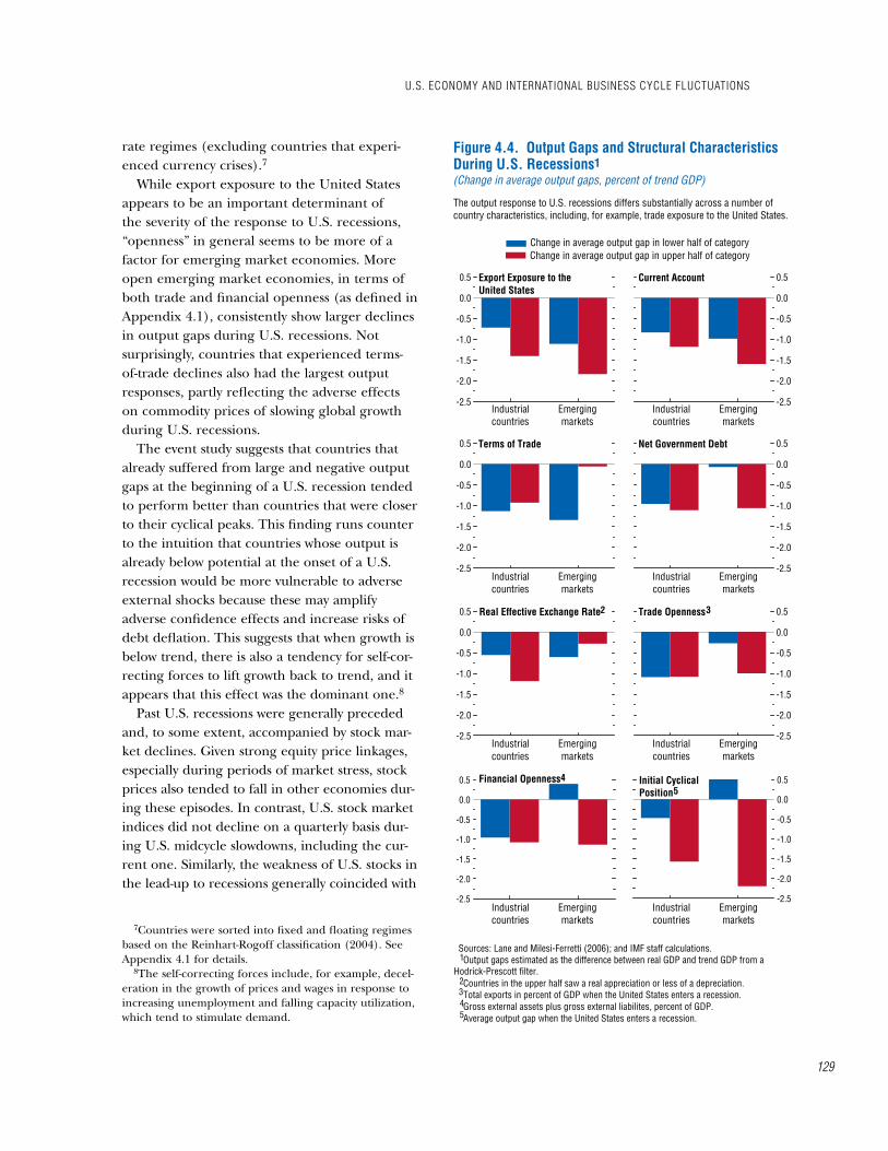
trade linkages, an important feature of past U.S. recessions has been that import growth turned sharply negative during every recession (Figure 4.3). In fact, U.S. imports are strongly procyclical, with a sensitivity that even exceeds that of private fixed investment. This reflects the relatively high import share of cyclically sensitive components of domestic final demand such as consumer durables and investment goods.6 Not surprisingly, countries with the greatest export exposure to the United States suffered the largest declines in output gaps (Figure 4.4).
6The share of imports of consumer durables and capital goods in total U.S. imports during 2005 was 48.9 percent, as compared with a share of these goods in domestic final demand of 7.9 percent during this period. Moreover, imports also include 31.3 percent of industrial raw materials, the demand for which is also cyclically sensitive.
table 4.4. u.S. Downturns and global growth
Recessions1 Slowdowns2 All All _______________________________________ _____________ 1974–75 1980 1982 1991 2001 1986 1995 Recessions Slowdowns
Change in GDP growth (median for region)
United States –6.1 –3.4 –4.5 –2.1 –2.9 –0.7 –1.5 –3.8 –1.1Other industrial countries –5.4 –1.5 0.4 –1.3 –2.0 –0.1 –0.3 –2.0 –0.1Latin America –3.2 –0.8 –3.9 1.1 –1.8 1.9 — –1.7 0.9Middle East and North Africa 1.2 –1.0 –3.3 0.8 –0.7 –0.2 0.7 –0.6 0.3Emerging Asia –3.5 –0.3 –1.5 –0.1 –1.1 0.9 0.3 –1.3 0.6Sub-Saharan Africa –0.5 — 1.0 — 0.6 –0.6 1.9 0.2 0.7Emerging Europe and CIS . . . . . . . . . –6.9 –0.3 . . . 3.8 –3.6 3.8
Ratio of median growth changes to U.S. growth changes (percent)
Other industrial countries 90 44 –10 61 69 –17 20 51 1Latin America 52 22 87 –53 61 –279 –1 34 –140Middle East and North Africa –20 30 74 –38 24 28 –47 14 –9Emerging Asia 57 10 33 4 37 –131 –16 28 –74Sub-Saharan Africa 9 –1 –23 0 –19 83 –123 –7 –20Emerging Europe and CIS . . . . . . . . . 335 11 . . . –250 173 –250
Percent of countries experiencing growth declines
Other industrial countries 91 64 45 73 91 45 55 73 50Latin America 77 62 90 37 83 33 47 70 40Middle East and North Africa 40 57 60 40 53 53 47 50 50Emerging Asia 72 56 78 53 84 47 42 68 45Sub-Saharan Africa 53 50 46 50 35 58 25 47 41Emerging Europe and CIS . . . . . . . . . 93 60 . . . 17 76 17
Source: IMF staff calculations.Note: CIS = Commonwealth of Independent States.1Year during which most of the impact on U.S. growth was recorded. Actual National Bureau of Economic Research (NBER) recession data
may slightly differ.2Midcycle slowdowns are defined as periods during which U.S. output was below potential (as determined by a Hodrick-Prescott filter) and
which were not considered recessions by the NBER. Specifically, the periods covered are 1986 and 1995.
u.S. economy anD international buSineSS cycle FluctuationS
127
chapter 4 Decoupling the train? SpilloverS anD cycleS in the global economy
128
For the transmission through trade channels, the behavior of the U.S. dollar during recessions also mattered. For example, the decrease in U.S. import growth during the 1982 recession was similar to that observed during the 1990–91 and 2001 recessions even though the 1982 recession was significantly deeper. This partly reflected the strong appreciation of the U.S. dollar in 1982, as monetary policy was tightened sharply to curb inflation. As a result, the competitiveness of U.S. trading partners improved, thereby buffering these economies from the U.S. recession and from the adverse effects of higher global real interest rates.
Industrial countries whose exchange rates depreciated during U.S. recessions tended to experience small growth declines while the opposite was true for emerging economies. This contrast is partly explained by the currency crises experienced by some emerging market economies during U.S. recessions, reflecting not only the external debt sustainability issues that emerged with terms-of-trade losses during these episodes (noted below), but also some-times higher U.S. interest rates and concurrent reversals of capital flows to emerging markets (Box 4.2). A related aspect is that most emerg-ing markets have external debt liabilities that are denominated in a foreign currency, typically in U.S. dollars, which can make them vulner-able to the increase in the debt-service burden associated with currency devaluations or depre-ciations. Such “balance sheet” effects also help explain why emerging economies with high ratios of public debt to GDP, which tend to be highly correlated with the external debt burden, experienced greater declines in output gaps than countries with lower debt ratios. These observations highlight the important role of eco-nomic vulnerabilities in determining how other countries are affected by U.S. recessions.
The evidence from the event study also sug-gests that exchange rate flexibility was helpful in mitigating adverse external effects during U.S. recessions, as countries with flexible exchange rate regimes, on average, experienced smaller growth declines than those with fixed exchange
1971 74 77 80 83 86 89 92 95 98 2001 04-20
-10
0
10
20
30
1971 74 77 80 83 86 89 92 95 98 2001 0470
80
90
100
110
120
130
140
150
1971 74 77 80 83 86 89 92 95 98 2001 040
20
40
60
80
100
120
1971 74 77 80 83 86 89 92 95 98 2001 040
3
6
9
12
15
18
Figure 4.3. United States: Real Imports, Real Effective Exchange Rate, Real Stock Returns, and Interest Rates During Recessions and Slowdowns
Sources: U.S. Bureau of Economic Analysis; Board of Governors of the Federal Reserve System; The Wall Street Journal ; and IMF staff calculations. S&P 500 index deflated by consumer price index. Yield on 10-year treasury bonds at constant maturity.
1
U.S. imports fell sharply in every recession while U.S. stock prices tended to decline, reflecting higher risk premia and declining corporate profitability. In contrast, imports registered a moderation in growth during slowdowns while stock prices remained relatively unaffected.
2
Performance over recession cycle U.S. recessionU.S. slowdownPerformance over slowdown cycle
Real Import Growth(percent)
Real Effective Exchange Rate(index 2000 = 100)
Real Stock Market Performance (index 2000 = 100)
Long-Term Interest Rates (percent)
1
2
rate regimes (excluding countries that experi-enced currency crises).7
While export exposure to the United States appears to be an important determinant of the severity of the response to U.S. recessions, “openness” in general seems to be more of a factor for emerging market economies. More open emerging market economies, in terms of both trade and financial openness (as defined in Appendix 4.1), consistently show larger declines in output gaps during U.S. recessions. Not surprisingly, countries that experienced terms-of-trade declines also had the largest output responses, partly reflecting the adverse effects on commodity prices of slowing global growth during U.S. recessions.
The event study suggests that countries that already suffered from large and negative output gaps at the beginning of a U.S. recession tended to perform better than countries that were closer to their cyclical peaks. This finding runs counter to the intuition that countries whose output is already below potential at the onset of a U.S. recession would be more vulnerable to adverse external shocks because these may amplify adverse confidence effects and increase risks of debt deflation. This suggests that when growth is below trend, there is also a tendency for self-cor-recting forces to lift growth back to trend, and it appears that this effect was the dominant one.8
Past U.S. recessions were generally preceded and, to some extent, accompanied by stock mar-ket declines. Given strong equity price linkages, especially during periods of market stress, stock prices also tended to fall in other economies dur-ing these episodes. In contrast, U.S. stock market indices did not decline on a quarterly basis dur-ing U.S. midcycle slowdowns, including the cur-rent one. Similarly, the weakness of U.S. stocks in the lead-up to recessions generally coincided with
7Countries were sorted into fixed and floating regimes based on the Reinhart-Rogoff classification (2004). See Appendix 4.1 for details.
8The self-correcting forces include, for example, decel-eration in the growth of prices and wages in response to increasing unemployment and falling capacity utilization, which tend to stimulate demand.
-2.5
-2.0
-1.5
-1.0
-0.5
0.0
0.5
Sources: Lane and Milesi-Ferretti (2006); and IMF staff calculations. Output gaps estimated as the difference between real GDP and trend GDP from a Hodrick-Prescott filter. Countries in the upper half saw a real appreciation or less of a depreciation. Total exports in percent of GDP when the United States enters a recession. Gross external assets plus gross external liabilites, percent of GDP. Average output gap when the United States enters a recession.
1
The output response to U.S. recessions differs substantially across a number of country characteristics, including, for example, trade exposure to the United States.
Change in average output gap in lower half of categoryChange in average output gap in upper half of category
Export Exposure to the United States
Industrialcountries
Emergingmarkets
-2.5
-2.0
-1.5
-1.0
-0.5
0.0
0.5Current Account
Industrialcountries
Emergingmarkets
Industrialcountries
Emergingmarkets
Industrialcountries
Emergingmarkets
-2.5
-2.0
-1.5
-1.0
-0.5
0.0
0.5 Terms of Trade
Industrialcountries
Emergingmarkets
-2.5
-2.0
-1.5
-1.0
-0.5
0.0
0.5Net Government Debt
Industrialcountries
Emergingmarkets
-2.5
-2.0
-1.5
-1.0
-0.5
0.0
0.5 Real Effective Exchange Rate
Industrialcountries
Emergingmarkets
-2.5
-2.0
-1.5
-1.0
-0.5
0.0
0.5Trade Openness
Industrialcountries
Emergingmarkets
-2.5
-2.0
-1.5
-1.0
-0.5
0.0
0.5 Financial Openness
-2.5
-2.0
-1.5
-1.0
-0.5
0.0
0.5Initial Cyclical Position
4
3
5
Figure 4.4. Output Gaps and Structural Characteristics During U.S. Recessions(Change in average output gaps, percent of trend GDP)
1
2345
2
u.S. economy anD international buSineSS cycle FluctuationS
129
chapter 4 Decoupling the train? SpilloverS anD cycleS in the global economy
130
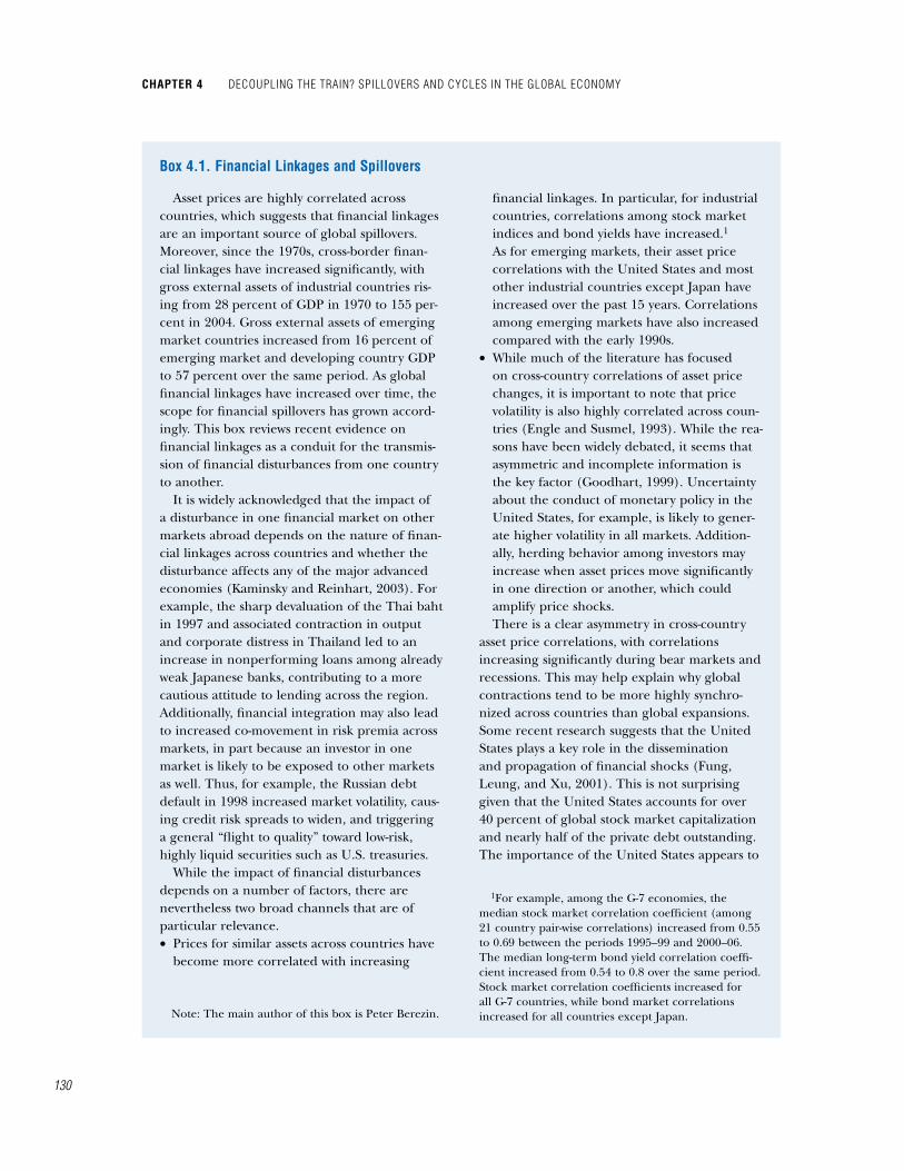
Asset prices are highly correlated across countries, which suggests that financial linkages are an important source of global spillovers. Moreover, since the 1970s, cross-border finan-cial linkages have increased significantly, with gross external assets of industrial countries ris-ing from 28 percent of GDP in 1970 to 155 per-cent in 2004. Gross external assets of emerging market countries increased from 16 percent of emerging market and developing country GDP to 57 percent over the same period. As global financial linkages have increased over time, the scope for financial spillovers has grown accord-ingly. This box reviews recent evidence on financial linkages as a conduit for the transmis-sion of financial disturbances from one country to another.
It is widely acknowledged that the impact of a disturbance in one financial market on other markets abroad depends on the nature of finan-cial linkages across countries and whether the disturbance affects any of the major advanced economies (Kaminsky and Reinhart, 2003). For example, the sharp devaluation of the Thai baht in 1997 and associated contraction in output and corporate distress in Thailand led to an increase in nonperforming loans among already weak Japanese banks, contributing to a more cautious attitude to lending across the region. Additionally, financial integration may also lead to increased co-movement in risk premia across markets, in part because an investor in one market is likely to be exposed to other markets as well. Thus, for example, the Russian debt default in 1998 increased market volatility, caus-ing credit risk spreads to widen, and triggering a general “flight to quality” toward low-risk, highly liquid securities such as U.S. treasuries.
While the impact of financial disturbances depends on a number of factors, there are nevertheless two broad channels that are of particular relevance. • Prices for similar assets across countries have
become more correlated with increasing
financial linkages. In particular, for industrial countries, correlations among stock market indices and bond yields have increased.1 As for emerging markets, their asset price correlations with the United States and most other industrial countries except Japan have increased over the past 15 years. Correlations among emerging markets have also increased compared with the early 1990s.
• While much of the literature has focused on cross-country correlations of asset price changes, it is important to note that price volatility is also highly correlated across coun-tries (Engle and Susmel, 1993). While the rea-sons have been widely debated, it seems that asymmetric and incomplete information is the key factor (Goodhart, 1999). Uncertainty about the conduct of monetary policy in the United States, for example, is likely to gener-ate higher volatility in all markets. Addition-ally, herding behavior among investors may increase when asset prices move significantly in one direction or another, which could amplify price shocks. There is a clear asymmetry in cross-country
asset price correlations, with correlations increasing significantly during bear markets and recessions. This may help explain why global contractions tend to be more highly synchro-nized across countries than global expansions. Some recent research suggests that the United States plays a key role in the dissemination and propagation of financial shocks (Fung, Leung, and Xu, 2001). This is not surprising given that the United States accounts for over 40 percent of global stock market capitalization and nearly half of the private debt outstanding. The importance of the United States appears to
1For example, among the G-7 economies, the median stock market correlation coefficient (among 21 country pair-wise correlations) increased from 0.55 to 0.69 between the periods 1995–99 and 2000–06. The median long-term bond yield correlation coeffi-cient increased from 0.54 to 0.8 over the same period. Stock market correlation coefficients increased for all G-7 countries, while bond market correlations increased for all countries except Japan.
box 4.1. Financial linkages and Spillovers
Note: The main author of this box is Peter Berezin.
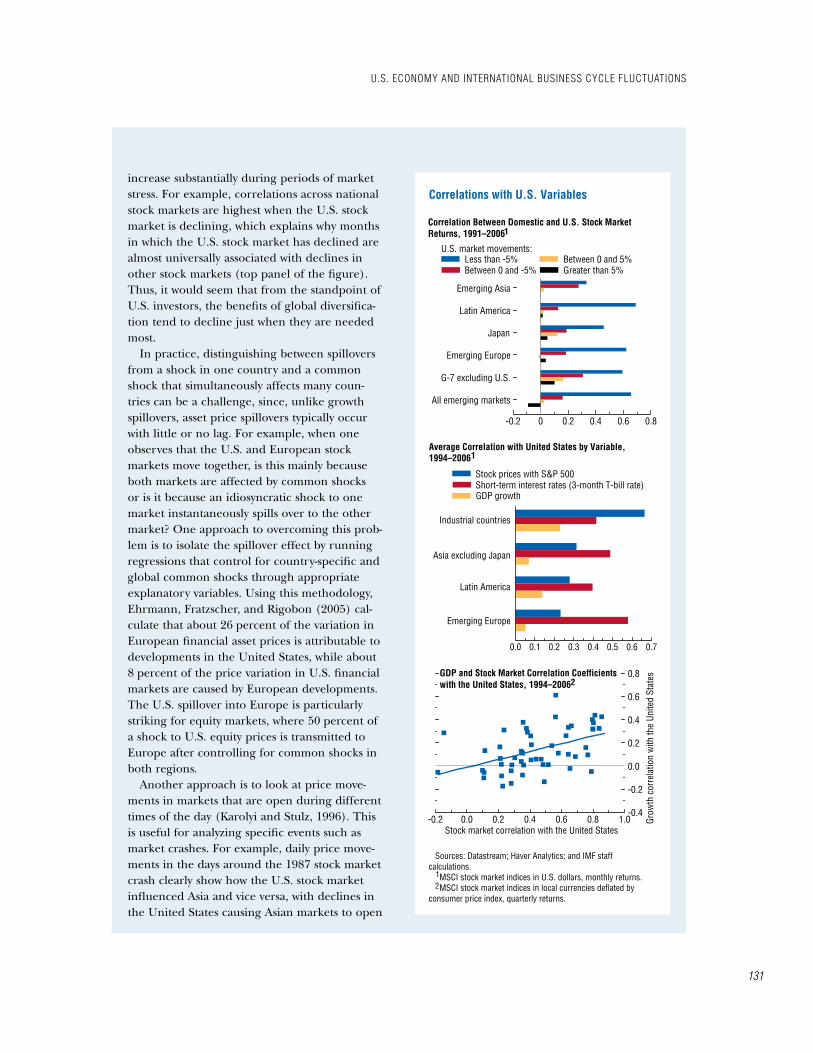
increase substantially during periods of market stress. For example, correlations across national stock markets are highest when the U.S. stock market is declining, which explains why months in which the U.S. stock market has declined are almost universally associated with declines in other stock markets (top panel of the figure). Thus, it would seem that from the standpoint of U.S. investors, the benefits of global diversifica-tion tend to decline just when they are needed most.
In practice, distinguishing between spillovers from a shock in one country and a common shock that simultaneously affects many coun-tries can be a challenge, since, unlike growth spillovers, asset price spillovers typically occur with little or no lag. For example, when one observes that the U.S. and European stock markets move together, is this mainly because both markets are affected by common shocks or is it because an idiosyncratic shock to one market instantaneously spills over to the other market? One approach to overcoming this prob-lem is to isolate the spillover effect by running regressions that control for country-specific and global common shocks through appropriate explanatory variables. Using this methodology, Ehrmann, Fratzscher, and Rigobon (2005) cal-culate that about 26 percent of the variation in European financial asset prices is attributable to developments in the United States, while about 8 percent of the price variation in U.S. financial markets are caused by European developments. The U.S. spillover into Europe is particularly striking for equity markets, where 50 percent of a shock to U.S. equity prices is transmitted to Europe after controlling for common shocks in both regions.
Another approach is to look at price move-ments in markets that are open during different times of the day (Karolyi and Stulz, 1996). This is useful for analyzing specific events such as market crashes. For example, daily price move-ments in the days around the 1987 stock market crash clearly show how the U.S. stock market influenced Asia and vice versa, with declines in the United States causing Asian markets to open
Emerging Asia
Latin America
Japan
Emerging Europe
G-7 excluding U.S.
All emerging markets
-0.2 0 0.2 0.4 0.6 0.8
Correlations with U.S. Variables
Sources: Datastream; Haver Analytics; and IMF staff calculations. MSCI stock market indices in U.S. dollars, monthly returns. MSCI stock market indices in local currencies deflated by consumer price index, quarterly returns.
Box. 4.1 Figure 1
Correlation Between Domestic and U.S. Stock Market Returns, 1991–2006
Less than -5% Between 0 and 5%Greater than 5%
0.0 0.1 0.2 0.3 0.4 0.5 0.6 0.7
Average Correlation with United States by Variable, 1994–2006
Industrial countries
Asia excluding Japan
Latin America
Emerging Europe
-0.2 0.0 0.2 0.4 0.6 0.8 1.0-0.4
-0.2
0.0
0.2
0.4
0.6
0.8GDP and Stock Market Correlation Coefficients with the United States, 1994–2006
Stock prices with S&P 500Short-term interest rates (3-month T-bill rate)GDP growth
U.S. market movements:
Grow
th c
orre
latio
n w
ith th
e Un
ited
Stat
es
Stock market correlation with the United States
1
1
2
21
Between 0 and -5%
u.S. economy anD international buSineSS cycle FluctuationS
131
chapter 4 Decoupling the train? SpilloverS anD cycleS in the global economy
132
significant declines in corporate earnings while, during slowdowns, corporate earnings generally have not declined, including at present.
An event analysis was also performed for slowdowns. Unlike for recessions, however, no clear-cut patterns emerged. This finding does not mean that the factors that shape the global spillovers during recessions are irrelevant during slowdowns. It would seem more plausible that the underlying U.S. disturbances were small in scale during slowdowns, which makes the identi-fication of such factors through simple descrip-tive analysis more difficult, as spillovers have been overshadowed by other developments.
growth Fluctuations in major currency areas and Spillovers: two econometric assessments
Moving beyond the event analysis, economet-ric estimates of the effects on output elsewhere of disturbances to growth in major advanced economies, including in particular the United States, can provide a more rigorous assess-ment of the cross-border growth spillovers. In approaching this exercise, it is necessary to recognize that any analysis at the global level faces trade-offs between the sophistication of the modeling framework—notably, the extent to which the disturbances have a precise economic interpretation attached to them—and availability of data. This section employs two different mod-
eling frameworks to arrive at robust conclusions while maintaining some coverage for a large number of countries.
A Broad Cross-Country Analysis
To start with an approach that can be applied to a broad cross-section of countries, a series of panel regressions was estimated relating growth in domestic output per capita to various com-binations of U.S. growth, euro area growth, and Japanese growth. The coefficients on these foreign growth variables provide a measure of the magnitude of spillovers. To reduce the likelihood that the estimated spillovers reflect common unobserved shocks, the set of explana-tory variables was expanded to include several controls: terms-of-trade changes; a short-term interest rate (the U.S. dollar London Interbank Offered Rate, or LIBOR); controls for the Latin American debt and Tequila crises, the Asian financial crises of 1997–98, and the Argentine crisis of 2001–02; country fixed effects; initial GDP; and population growth. The sample includes up to 130 advanced economies and developing countries, covering all World Eco-nomic Outlook regions, and uses annual data over 1970–2005 (see Appendix 4.1 for details).
Even the simplest specification finds signifi-cant cross-country spillovers from growth in the United States, the euro area, and Japan (Table 4.5, column 1). On average, the United
lower and intraday movements in Asian markets strongly influencing the following day’s open in New York.
Comparing financial market linkages and business cycle linkages, stock prices and inter-est rates have tended to be more correlated across countries than GDP growth rates (see the figure). There is also a positive relationship between how synchronized a country’s stock market is with the United States and how syn-chronized its business cycle is with the United States. Additionally, countries that are more
financially open tend to have stock markets that are more synchronized with the United States. These facts suggest that financial linkages do indeed play an important role in transmit-ting shocks that affect real variables, and that continued financial integration over time may amplify financial spillovers across countries. This may be particularly true for emerging market economies as their financial sectors continue to become larger and more integrated with the global financial system (Cuadro Sáez, Fratzscher, and Thimann, 2007).
box 4.1 (concluded)
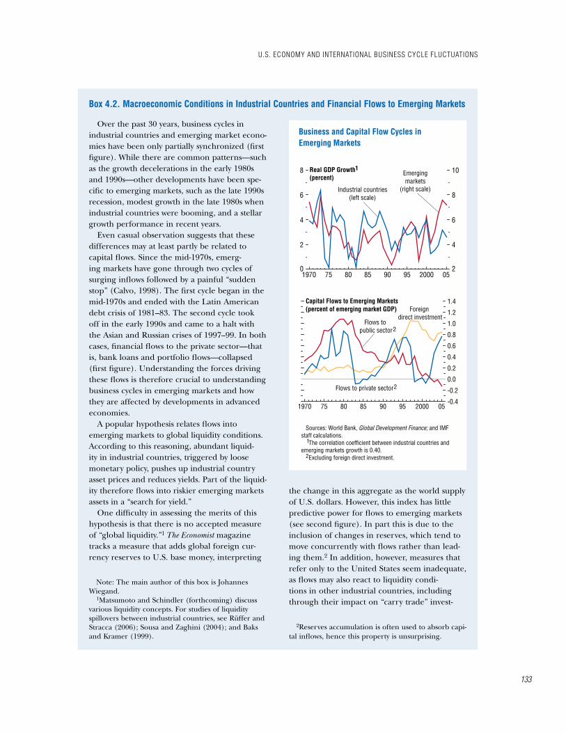
Over the past 30 years, business cycles in industrial countries and emerging market econo-mies have been only partially synchronized (first figure). While there are common patterns—such as the growth decelerations in the early 1980s and 1990s—other developments have been spe-cific to emerging markets, such as the late 1990s recession, modest growth in the late 1980s when industrial countries were booming, and a stellar growth performance in recent years.
Even casual observation suggests that these differences may at least partly be related to capital flows. Since the mid-1970s, emerg-ing markets have gone through two cycles of surging inflows followed by a painful “sudden stop” (Calvo, 1998). The first cycle began in the mid-1970s and ended with the Latin American debt crisis of 1981–83. The second cycle took off in the early 1990s and came to a halt with the Asian and Russian crises of 1997–99. In both cases, financial flows to the private sector—that is, bank loans and portfolio flows—collapsed (first figure). Understanding the forces driving these flows is therefore crucial to understanding business cycles in emerging markets and how they are affected by developments in advanced economies.
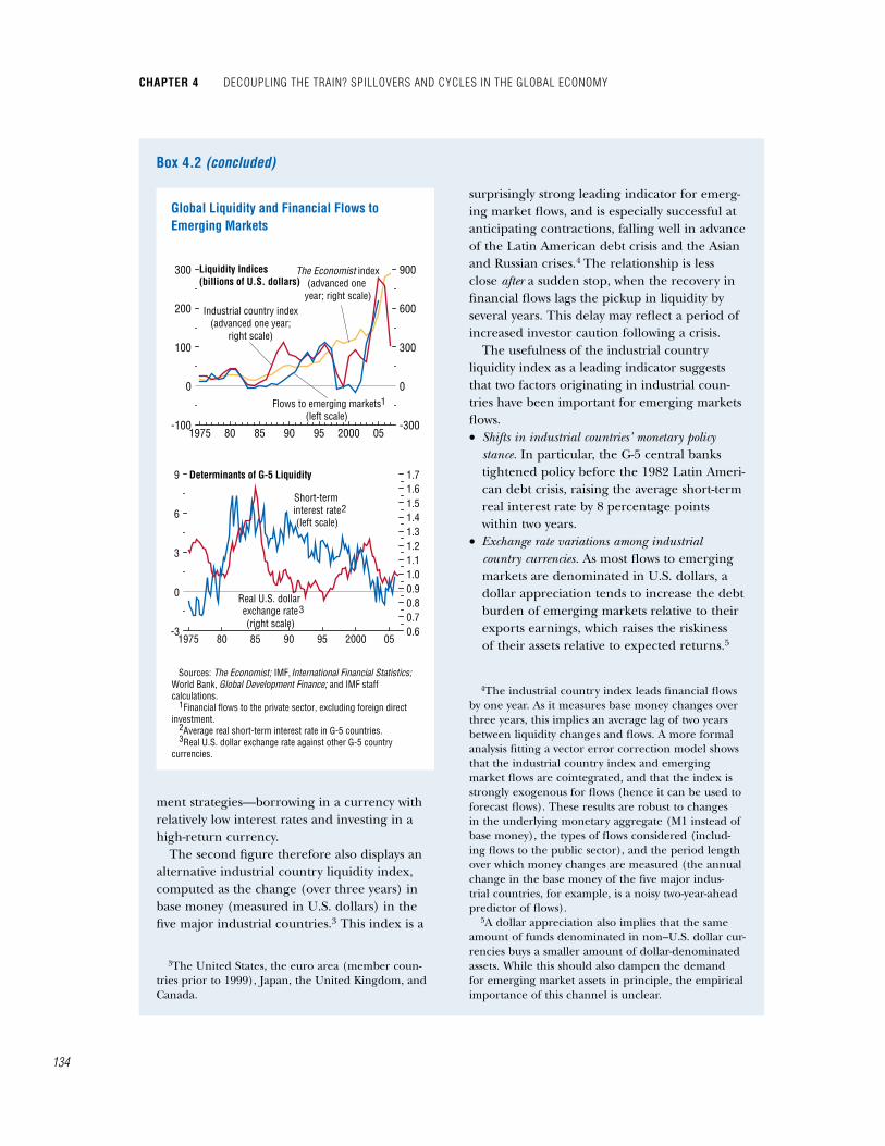
A popular hypothesis relates flows into emerging markets to global liquidity conditions. According to this reasoning, abundant liquid-ity in industrial countries, triggered by loose monetary policy, pushes up industrial country asset prices and reduces yields. Part of the liquid-ity therefore flows into riskier emerging markets assets in a “search for yield.”
One difficulty in assessing the merits of this hypothesis is that there is no accepted measure of “global liquidity.”1 The Economist magazine tracks a measure that adds global foreign cur-rency reserves to U.S. base money, interpreting
Note: The main author of this box is Johannes Wiegand.
1Matsumoto and Schindler (forthcoming) discuss various liquidity concepts. For studies of liquidity spillovers between industrial countries, see Rüffer and Stracca (2006); Sousa and Zaghini (2004); and Baks and Kramer (1999).
the change in this aggregate as the world supply of U.S. dollars. However, this index has little predictive power for flows to emerging markets (see second figure). In part this is due to the inclusion of changes in reserves, which tend to move concurrently with flows rather than lead-ing them.2 In addition, however, measures that refer only to the United States seem inadequate, as flows may also react to liquidity condi-tions in other industrial countries, including through their impact on “carry trade” invest-
2Reserves accumulation is often used to absorb capi-tal inflows, hence this property is unsurprising.
box 4.2. macroeconomic conditions in industrial countries and Financial Flows to emerging markets
1970 75 80 85 90 95 2000 050
2
4
6
8
2
4
6
8
10
1970 75 80 85 90 95 2000 05-0.4
-0.2
0.0
0.2
0.4
0.6
0.8
1.0
1.2
1.4
Business and Capital Flow Cycles in Emerging Markets
Sources: World Bank, Global Development Finance; and IMF staff calculations. The correlation coefficient between industrial countries and emerging markets growth is 0.40. Excluding foreign direct investment.
Box. 4.2 Figure 1
Real GDP Growth(percent)
Emergingmarkets
(right scale)Industrial countries(left scale)
Capital Flows to Emerging Markets(percent of emerging market GDP) Foreign
direct investment
2
Flows to public sector
1
Flows to private sector
2
1
2
u.S. economy anD international buSineSS cycle FluctuationS
133
chapter 4 Decoupling the train? SpilloverS anD cycleS in the global economy
134
ment strategies—borrowing in a currency with relatively low interest rates and investing in a high-return currency.
The second figure therefore also displays an alternative industrial country liquidity index, computed as the change (over three years) in base money (measured in U.S. dollars) in the five major industrial countries.3 This index is a
3The United States, the euro area (member coun-tries prior to 1999), Japan, the United Kingdom, and Canada.
surprisingly strong leading indicator for emerg-ing market flows, and is especially successful at anticipating contractions, falling well in advance of the Latin American debt crisis and the Asian and Russian crises.4 The relationship is less close after a sudden stop, when the recovery in financial flows lags the pickup in liquidity by several years. This delay may reflect a period of increased investor caution following a crisis.
The usefulness of the industrial country liquidity index as a leading indicator suggests that two factors originating in industrial coun-tries have been important for emerging markets flows.• Shifts in industrial countries’ monetary policy
stance. In particular, the G-5 central banks tightened policy before the 1982 Latin Ameri-can debt crisis, raising the average short-term real interest rate by 8 percentage points within two years.
• Exchange rate variations among industrial country currencies. As most flows to emerging markets are denominated in U.S. dollars, a dollar appreciation tends to increase the debt burden of emerging markets relative to their exports earnings, which raises the riskiness of their assets relative to expected returns.5
4The industrial country index leads financial flows by one year. As it measures base money changes over three years, this implies an average lag of two years between liquidity changes and flows. A more formal analysis fitting a vector error correction model shows that the industrial country index and emerging market flows are cointegrated, and that the index is strongly exogenous for flows (hence it can be used to forecast flows). These results are robust to changes in the underlying monetary aggregate (M1 instead of base money), the types of flows considered (includ-ing flows to the public sector), and the period length over which money changes are measured (the annual change in the base money of the five major indus-trial countries, for example, is a noisy two-year-ahead predictor of flows).
5A dollar appreciation also implies that the same amount of funds denominated in non–U.S. dollar cur-rencies buys a smaller amount of dollar-denominated assets. While this should also dampen the demand for emerging market assets in principle, the empirical importance of this channel is unclear.
1975 80 85 90 95 2000 05-100
0
100
200
300
-300
0
300
600
900The Economist index(advanced one
year; right scale)
1975 80 85 90 95 2000 05-3
0
3
6
9
0.60.70.80.91.01.11.21.31.41.51.61.7
Global Liquidity and Financial Flows to Emerging Markets
Sources: The Economist; IMF, International Financial Statistics;World Bank, Global Development Finance; and IMF staff calculations. Financial flows to the private sector, excluding foreign direct investment. Average real short-term interest rate in G-5 countries. Real U.S. dollar exchange rate against other G-5 country currencies.
Box. 4.2 Figure 2
Liquidity Indices(billions of U.S. dollars)
Flows to emerging markets(left scale)
1
Industrial country index(advanced one year;
right scale)
Determinants of G-5 Liquidity
Short-term interest rate(left scale)
2
Real U.S. dollar exchange rate(right scale)
3
1
23
box 4.2 (concluded)
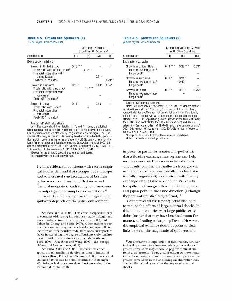
States exerts the greatest impact. In particular, a 1 percentage point decline in U.S. growth is associated with an average 0.16 percentage point drop in growth across the sample, substantially larger than the spillovers from the euro area or Japan.
Following the analysis in the previous section, a natural hypothesis is that the magnitude of spillovers will be closely linked to the strength of trade linkages among economies. Indeed, the results confirm that growth in both the United States and the euro area lead to spillovers into other countries precisely to the extent that these other countries trade with, respectively, the United States and the euro area (Table 4.5, column 2).9 Quantitatively, the results imply that, if a country’s total trade with the United States
9Trade intensity with any of the three major currency areas was measured as the ratio of total trade (exports plus imports with that area) to a country’s GDP. Growth in the United States, euro area, and Japan, respectively, was then interacted with these trade ratios. Controlling for these interactions, the level terms proved statistically insignificant.
rises by 10 percentage points of GDP, then the impact of a 1 percentage point increase in U.S. growth on domestic growth rises by about 0.1 per-centage point. There is also some evidence that the magnitude of spillovers from U.S. growth is significantly larger into those countries that are more financially integrated with the United States (Table 4.5, column 3).10
Given the rapid, ongoing increases in trade and financial integration over the period, the above findings imply that spillovers should rise over time. Indeed, complementary results confirm that spillovers from growth in at least the United States were significantly higher in the post-1987 half of the sample (Table 4.5, column
10Financial integration between any two countries, i and j, is measured by |(NFAi/GDPi) – (NFAj/GDPj)|. Imbs (2004, p. 728) argues that “pairs of countries with intense capital flows should display different (or even opposite) net external positions. Two countries with massively positive (negative) net foreign assets holdings will both tend to be issuers (recipients) of capital flows, and should experience less bilateral flows than two countries where one is structurally in surplus and the other in deficit.” See Appendix 4.1 for details of other measures used.
Large U.S. dollar appreciations preceded both the Latin American and Asian crises. In 1995, for example, the dollar surged, espe-cially against the Japanese yen, after depreci-ating for almost a decade. Hence, East Asian economies—whose currencies were mostly pegged to the dollar—lost competitiveness without a compensating drop in their refi-nancing costs.6
Looking forward, growth in the industrial country liquidity index started to slow in 2005, reflecting monetary tightening by the major central banks. Taken at face value, this would suggest a reduction in emerging market flows going forward. However, more than half of the fall owes to the phasing out of the Bank of Japan’s “quantitative easing” policy. This high-
6See Ueda (1998), for example, for a more detailed discussion.
lights the question of how important Japan’s highly accommodating monetary stance has been for emerging markets recently. While pri-vate outflows from Japan have been large in the past three years, little is known about the extent to which they have been channeled to emerging markets, either directly or indirectly by promot-ing carry trades.7
Among recipient regions, emerging Europe, which has received about half of financial flows to emerging markets since 2003, seems most vulnerable to a flow reversal.8 Importantly, in many of these countries, external liabilities are denominated in euros rather than in dollars. A stronger euro could therefore be more of a con-cern going forward than a stronger U.S. dollar.
7See the April 2007 Global Financial Stability Report. 8See Box 1.1 of the September 2006 World Economic
Outlook.
u.S. economy anD international buSineSS cycle FluctuationS
135
chapter 4 Decoupling the train? SpilloverS anD cycleS in the global economy
136
4). This evidence is consistent with recent empir-ical studies that find that stronger trade linkages lead to increased synchronization of business cycles across countries11 and that increased financial integration leads to higher cross-coun-try output (and consumption) correlations.12
It is worthwhile asking how the magnitude of spillovers depends on the policy environment
11See Kose and Yi (2006). This effect is especially large in countries with strong intra-industry trade linkages and more similar sectoral structures (see Imbs, 2004; and Calderón, Chong, and Stein, 2007). Other studies report that increased intraregional trade volumes, especially in the form of intra-industry trade, have been an important factor in explaining the degree of business cycle synchro-nization within North America (Kose, Meredith, and Towe, 2005), Asia (Shin and Wang, 2003), and Europe (Böwer and Guillemineau, 2006).
12See Imbs (2004 and 2006). However, this effect appears much smaller in developing than in industrial countries (Kose, Prasad, and Terrones, 2003). Jansen and Stokman (2004) also find that countries with stronger FDI linkages had more correlated business cycles in the second half of the 1990s.
in place. In particular, a natural hypothesis is that a floating exchange rate regime may help insulate countries from some external shocks. The results confirm that spillovers from growth in the euro area are much smaller (indeed, sta-tistically insignificant) in countries with floating exchange rates (Table 4.6, column 2). Results for spillovers from growth in the United States and Japan point in the same direction (although they are not statistically significant).13
Countercyclical fiscal policy could also help to reduce the effects of large external shocks. In this context, countries with large public sector debts (or deficits) may have less fiscal room for maneuver, leading to larger spillovers. However, the empirical evidence does not point to clear links between the magnitude of spillovers and
13An alternative interpretation of these results, however, is that those countries whose underlying shocks display greater correlation may choose to peg for “optimal cur-rency area” reasons. Thus, greater output co-movements in fixed exchange rate countries may at least partly reflect greater correlation in the underlying shocks, rather than any inability of policy to offset the impact of external shocks.
table 4.5. growth and Spillovers (1)(Panel regression coefficients)
Dependent Variable: Growth in All Countries1 ___________________________Specification (1) (2) (3) (4)
Explanatory variables
Growth in United States 0.16*** – +Trade ratio with United States2 0.92**Financial integration with
United States2 0.31*Post-1987 indicator2 0.29**
Growth in euro area 0.10* 0.40* 0.34*Trade ratio with euro area2 1.1***Financial integration with
euro area2 –Post-1987 indicator2 –
Growth in Japan 0.11* 0.18* +Trade ratio with Japan2 +Financial integration
with Japan2 –Post-1987 indicator2 –
Source: IMF staff calculations.Note: See Appendix 4.1 for details. *, **, and *** denote statistical
significance at the 10 percent, 5 percent, and 1 percent level, respectively. For coefficients that are statistically insignificant, only the sign (+ or –) is shown. Other regressors include country fixed effects; initial GDP; popula-tion growth; growth in the terms of trade; the LIBOR; and controls for the Latin American debt and Tequila crises, the East Asian crises of 1997–98, and the Argentine crisis of 2001–02. Number of countries = 130, 125, 111, 130; number of observations = 3,741, 3,312, 2,900, 3,741.
1Except for the United States, the euro area, and Japan.2Interacted with indicated growth rate.
table 4.6. growth and Spillovers (2)(Panel regression coefficients)
Dependent Variable: Growth in All Other Countries1 _______________________Specification (1) (5) (6)
Explanatory variables
Growth in United States 0.16*** 0.22*** 0.23*Floating exchange rate2 –Large debt2 –
Growth in euro area 0.10* 0.24* –Floating exchange rate2 –0.40*Large debt2 +
Growth in Japan 0.11* 0.19* 0.25*Floating exchange rate2 –Large debt2 –
Source: IMF staff calculations.Note: See Appendix 4.1 for details. *, **, and *** denote statisti-
cal significance at the 10 percent, 5 percent, and 1 percent level, respectively. For coefficients that are statistically insignificant, only the sign (+ or –) is shown. Other regressors include country fixed effects; initial GDP; population growth; growth in the terms of trade; the LIBOR; and controls for the Latin American debt and Tequila crises, the East Asian crises of 1997–98, and the Argentine crisis of 2001–02. Number of countries = 130, 107, 96; number of observa-tions = 3,741, 2,935, 1,454.
1Except for the United States, the euro area, and Japan.2Interacted with indicated growth rate.
the size of debts or deficits (Table 4.6, column 3). One potential explanation is that fiscal policy may in fact have been procyclical in most devel-oping countries over the sample period (Kamin-sky, Reinhart, and Végh, 2004).
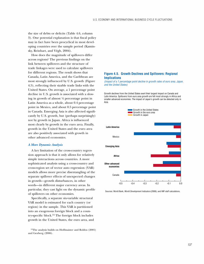
How does the magnitude of spillovers differ across regions? The previous findings on the link between spillovers and the structure of trade linkages were used to calculate spillovers for different regions. The result shows that Canada, Latin America, and the Caribbean are most strongly influenced by U.S. growth (Figure 4.5), reflecting their sizable trade links with the United States. On average, a 1 percentage point decline in U.S. growth is associated with a slow-ing in growth of almost ¼ percentage point in Latin America as a whole, about 0.4 percentage point in Mexico, and about 0.5 percentage point in Canada. Emerging Asia is also affected signifi-cantly by U.S. growth, but (perhaps surprisingly) not by growth in Japan. Africa is influenced most clearly by growth in the euro area. Finally, growth in the United States and the euro area are also positively associated with growth in other advanced economies.
A More Dynamic Analysis
A key limitation of the cross-country regres-sion approach is that it only allows for relatively simple interactions across countries. A more sophisticated analysis using a cross-country and cross-region set of vector auto regression (VAR) models allows more precise disentangling of the separate spillover effects of unexpected changes in growth—growth disturbances, in other words—in different major currency areas. In particular, they cast light on the dynamic profile of spillovers on other economies.
Specifically, a separate six-variable structural VAR model is estimated for each country (or region) in the sample. This VAR is partitioned into an exogenous foreign block and a coun-try-specific block.14 The foreign block includes growth in the United States, the euro area, and
14The analysis builds on Hoffmaister and Roldos (2001) and Genberg (2006).
Latin America
Emerging Asia
Africa
-0.5 -0.4 -0.3 -0.2 -0.1 0.0
Figure 4.5. Growth Declines and Spillovers: Regional Implications(Impact of a 1 percentage point decline in growth rates of euro area, Japan, and the United States)
Sources: World Bank, World Development Indicators (2006); and IMF staff calculations.
Growth declines from the United States exert their largest impact on Canada and Latin America. Spillovers from euro area growth are felt most strongly in Africa and smaller advanced economies. The impact of Japan's growth can be detected only in Asia.
Growth in the United StatesGrowth in the euro areaGrowth in Japan
Canada
Mexico
Other advancedeconomies
u.S. economy anD international buSineSS cycle FluctuationS
137
chapter 4 Decoupling the train? SpilloverS anD cycleS in the global economy
138
Japan, which are interrelated given the link-ages among them but are assumed not to be significantly affected by developments elsewhere. The country-specific block includes (country-specific) growth, inflation, and the percentage change in the real effective exchange rate. In addition, the equations in this block include the following control variables: the terms of trade; the LIBOR; and controls for the Latin Ameri-can debt and Tequila crises, the Asian financial crises of 1997–98, and the Argentine crisis of 2001–02. The sample includes 46 countries, both advanced and developing, as well as the corresponding regional averages,15 and uses quarterly data, typically available for 1991–2005 (see Appendix 4.1 for details).
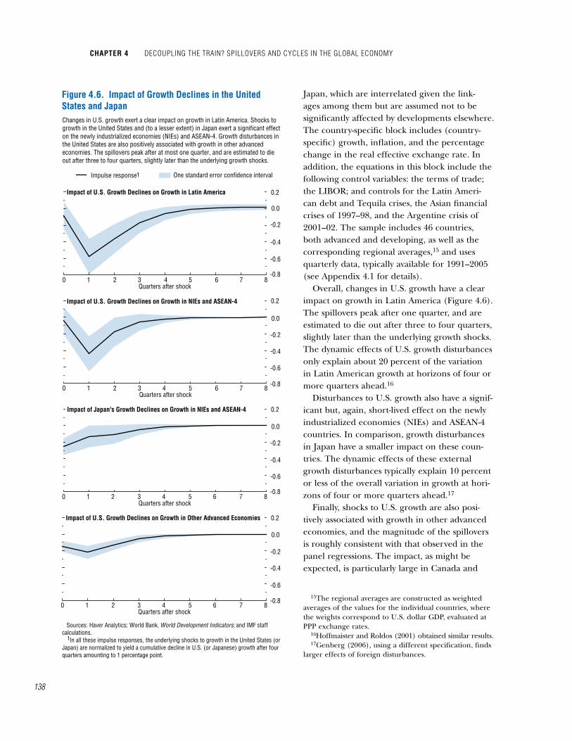
Overall, changes in U.S. growth have a clear impact on growth in Latin America (Figure 4.6). The spillovers peak after one quarter, and are estimated to die out after three to four quarters, slightly later than the underlying growth shocks. The dynamic effects of U.S. growth disturbances only explain about 20 percent of the variation in Latin American growth at horizons of four or more quarters ahead.16
Disturbances to U.S. growth also have a signif-icant but, again, short-lived effect on the newly industrialized economies (NIEs) and ASEAN-4 countries. In comparison, growth disturbances in Japan have a smaller impact on these coun-tries. The dynamic effects of these external growth disturbances typically explain 10 percent or less of the overall variation in growth at hori-zons of four or more quarters ahead.17
Finally, shocks to U.S. growth are also posi-tively associated with growth in other advanced economies, and the magnitude of the spillovers is roughly consistent with that observed in the panel regressions. The impact, as might be expected, is particularly large in Canada and
15The regional averages are constructed as weighted averages of the values for the individual countries, where the weights correspond to U.S. dollar GDP, evaluated at PPP exchange rates.
16Hoffmaister and Roldos (2001) obtained similar results.17Genberg (2006), using a different specification, finds
larger effects of foreign disturbances.
Figure 4.6. Impact of Growth Declines in the United States and JapanChanges in U.S. growth exert a clear impact on growth in Latin America. Shocks to growth in the United States and (to a lesser extent) in Japan exert a significant effect on the newly industrialized economies (NIEs) and ASEAN-4. Growth disturbances in the United States are also positively associated with growth in other advanced economies. The spillovers peak after at most one quarter, and are estimated to die out after three to four quarters, slightly later than the underlying growth shocks.
One standard error confidence intervalImpulse response1
Impact of U.S. Growth Declines on Growth in Latin America
-0.6
-0.8
-0.4
-0.2
0.0
0.2
-0.6
-0.8
-0.4
-0.2
0.0
0.2Impact of U.S. Growth Declines on Growth in NIEs and ASEAN-4
Impact of Japan's Growth Declines on Growth in NIEs and ASEAN-4
-0.6
-0.8
-0.4
-0.2
0.0
0.2
Impact of U.S. Growth Declines on Growth in Other Advanced Economies
-0.6
-0.8
-0.4
-0.2
0.0
0.2
1
Quarters after shock
Quarters after shock
Quarters after shock
Quarters after shock
Sources: Haver Analytics; World Bank, World Development Indicators; and IMF staff calculations. In all these impulse responses, the underlying shocks to growth in the United States (or Japan) are normalized to yield a cumulative decline in U.S. (or Japanese) growth after four quarters amounting to 1 percentage point.
0 1 2 3 4 5 6 7 8
0 1 2 3 4 5 6 7 8
0 1 2 3 4 5 6 7 8
0 1 2 3 4 5 6 7 8
in commodity exporters such as Australia and Norway. In general, the qualitative results from this dynamic analysis are fully consistent with the results from the panel regressions. That said, the precise quantitative estimates differ, reflect-ing differences in the methodologies, sample composition, and sample periods.
Four important messages emerge from the panel regressions and VAR analysis. First, growth in the United States (and other large econo-mies) can exert important spillovers on both advanced and developing economies. While gen-erally moderate in magnitude (but statistically significant), the spillovers can be substantial for regional trading partners. Second, the panel regression analysis indicates that the magnitude of the spillovers may have increased over time. Third, for many countries, external growth dis-turbances nevertheless seem less important than domestic factors in explaining overall volatil-ity. Fourth, the analysis suggests that a flexible exchange rate regime can in some cases help insulate economies from external shocks.
identifying common elements in international business cycle Fluctuations
How important are common elements in driving international business cycles and what are the underlying forces? The answer to this question has important implications for the interpretation of past episodes of strong busi-ness cycle synchronization—that is, episodes of strong co-movements in economic activity across countries—and for the prospects of such episodes occurring again. There could be three basic, not mutually exclusive, reasons accounting for these episodes. First, such episodes could pri-marily reflect common shocks, such as abrupt, unexpected changes in oil prices or sharp movements in asset prices in the major financial centers. Second, they could reflect the global spillovers from disturbances originating in one of the large economies. Third, these episodes could reflect correlated disturbances that could arise for a number of reasons, including, for example, the implementation of similar policies.
The approaches pursued so far in the chap-ter are not suited to identifying such common elements in national business cycles. To address this issue, a dynamic factor model was estimated that captures common factors in the fluctuations of real per capita output, private consumption, and investment over the 1960–2005 period in 93 countries.18 Specifically, the model decomposes fluctuations in these variables into four factors (see Appendix 4.2 for details):• A global factor captures the broad common ele-
ments in the fluctuations across countries. • Regional factors capture the common elements
in the cyclical fluctuations in the countries in a particular region. For the purposes of this chapter, the world was partitioned into seven regions: North America, Europe, Oceania, Asia, Latin America, Middle East and North Africa, and sub-Saharan Africa.
• Country-specific factors capture factors common to all variables in a particular country.
• Residual (“idiosyncratic”) factors capture elements in the fluctuations of an individual variable that cannot be attributed to the other factors. Table 4.7 shows the relative contributions of
the global, regional, country-specific, and idio-syncratic factors to the cyclical fluctuations in each region. The main findings are as follows:• The global factor generally plays a more
important role in explaining business cycles in industrial countries than in emerging market and developing countries. In indus-trial countries, this factor on average explains more than 15 percent of output fluctuations, with the contribution in the relatively larger industrial countries typically exceeding 20 per-cent. In contrast, in emerging market and other developing countries, the global factor explains less than 10 percent of the output fluctuations.
• Regional factors are most important in North America, Europe, and Asia, where they explain more than 20 percent of the output fluctuations. The regional factors capture well-
18This model builds on Kose, Otrok, and Whiteman (2003).
iDentiFying common elementS in international buSineSS cycle FluctuationS
139
chapter 4 Decoupling the train? SpilloverS anD cycleS in the global economy
140
known regional developments, including, for example, the 1997–98 Asian financial crises.
• Country-specific and idiosyncratic factors appear to play the most important role in the Middle East and North Africa and in sub-Saharan Africa, where they explain more than 80 percent of output variation.19 Figure 4.7 shows the estimated global factor
and illustrates how closely this factor matches the major peaks and troughs observed in global GDP growth over the past 45 years, including the recessions in 1974–75 and the early 1980s, the slowdown in the early 2000s, and the recent global recovery. Moreover, there is considerable overlap in the evolution of the global factor and U.S. growth, especially during U.S. recessions. In the early 1990s, however, the global factor reached a trough later than did U.S. output.
19See Chapter 2 of the April 2005 World Economic Out-look for a more detailed analysis.
This is consistent with the interpretation that the 1990–91 U.S. recession reflected more U.S.-spe-cific developments than usual, which were then transmitted to other countries, as noted earlier.
How has the importance of the global, regional, and country factors changed over time? To answer this question, the dynamic factor model was estimated over two periods, 1960–85 and 1986–2005.20 The results suggest that the global factor has, on average, played a less important role in the later period (see Table 4.7). At the same time, regional factors have become more important in regions where trade and financial linkages have increased substantially. In particular, in the later period, the regional factor has accounted for more than half of the output fluctuations in North America, and 38 and 41 percent of output fluctuations in Europe and Asia, respectively, compared with roughly 20 and 10 percent during the first period. In Latin America, however, the regional factor explains a lower share of output fluctuations in the second period than in the first one, suggesting that the region-specific common factors were primarily related to the buildup in external debt and subse-quent debt crises during the earlier period.
The total contribution of global and regional factors together to output fluctuations has, on average, remained similar between the two periods, except in emerging Asia, where it has increased.21 Since this total contribution of global and regional factors is a measure of the extent of co-movement across national business cycles, these results show that overall, national business cycles have not necessarily become more synchronized in general (Box 4.3).
20These subperiods capture a structural break in output volatility in several industrial countries. In addition, this break point is intuitively appealing in the sense that there has been a substantial increase in international trade and financial flows since the mid-1980s.
21In Asia, the regional factor also appears to pick up the influence of the East Asian financial crisis. When the model is estimated excluding the crisis years (1997 and 1998) in East Asia, the role of the regional factor in the second period appears to be less prominent, although it still explains a larger share of output fluctuations than in the first period.
table 4.7. contributions to output Fluctuations(Unweighted averages for each region; percent)
Factors _________________________________ Global Regional Country Idiosyncratic
1960–2005North America 16.9 51.7 14.8 16.6Western Europe 22.7 21.6 34.6 21.1Oceania 5.6 3.9 61.8 28.7Emerging Asia and Japan 7.0 21.9 47.4 23.7Latin America 9.1 16.6 48.6 25.7Sub-Saharan Africa 5.3 2.7 40.7 51.3Middle East and North Africa 6.3 6.3 53.8 33.6 1960–85
North America 31.4 36.4 15.7 16.5Western Europe 26.6 20.5 31.6 21.3Oceania 10.7 5.9 50.5 32.9Emerging Asia and Japan 10.6 9.5 50.5 29.4Latin America 16.2 19.4 41.2 23.2Sub-Saharan Africa 7.2 5.1 39.7 48.0Middle East and North Africa 8.9 5.1 49.1 36.9 1986–2005
North America 5.0 62.8 8.2 24.0Western Europe 5.6 38.3 27.6 28.5Oceania 9.4 25.9 31.1 33.6Emerging Asia and Japan 6.5 34.7 31.1 27.7Latin America 7.8 8.7 51.7 31.8Sub-Saharan Africa 6.7 4.7 37.3 51.3Middle East and North Africa 4.7 6.6 52.8 35.9
Source: IMF staff calculations.Note: The table shows the fraction of the variance of output growth
attributable to each factor.
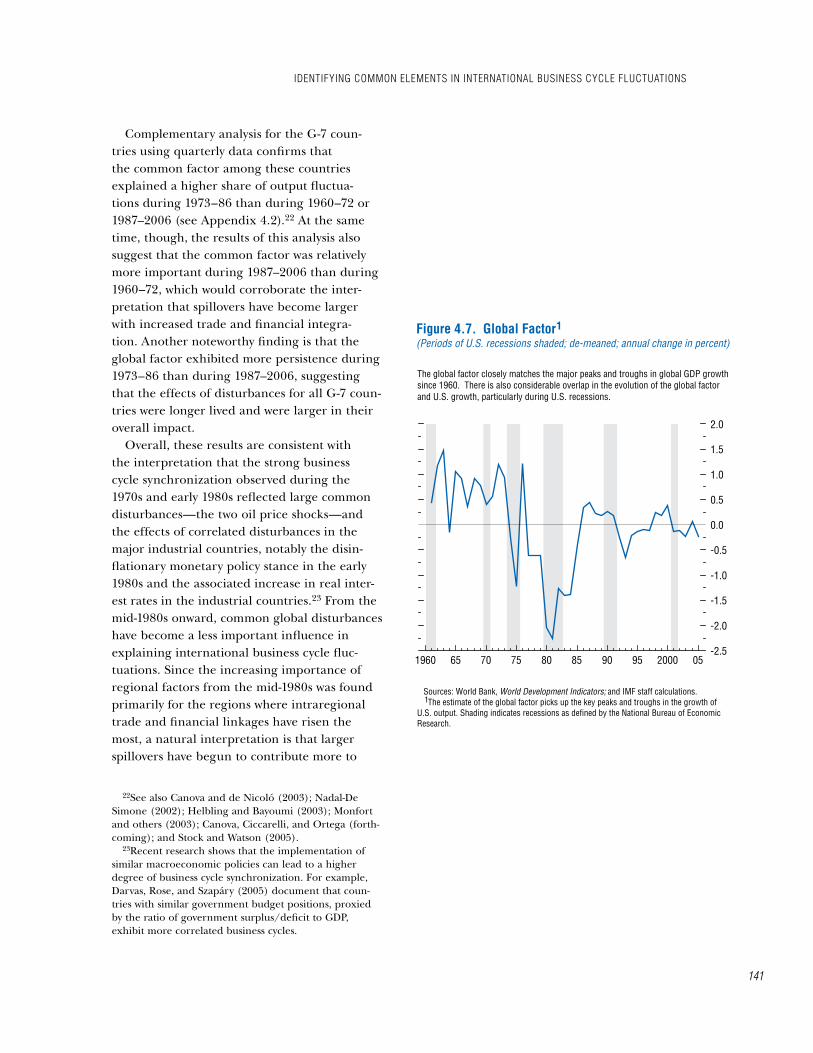
Complementary analysis for the G-7 coun-tries using quarterly data confirms that the common factor among these countries explained a higher share of output fluctua-tions during 1973–86 than during 1960–72 or 1987–2006 (see Appendix 4.2).22 At the same time, though, the results of this analysis also suggest that the common factor was relatively more important during 1987–2006 than during 1960–72, which would corroborate the inter-pretation that spillovers have become larger with increased trade and financial integra-tion. Another noteworthy finding is that the global factor exhibited more persistence during 1973–86 than during 1987–2006, suggesting that the effects of disturbances for all G-7 coun-tries were longer lived and were larger in their overall impact.
Overall, these results are consistent with the interpretation that the strong business cycle synchronization observed during the 1970s and early 1980s reflected large common disturbances—the two oil price shocks—and the effects of correlated disturbances in the major industrial countries, notably the disin-flationary monetary policy stance in the early 1980s and the associated increase in real inter-est rates in the industrial countries.23 From the mid-1980s onward, common global disturbances have become a less important influence in explaining international business cycle fluc-tuations. Since the increasing importance of regional factors from the mid-1980s was found primarily for the regions where intraregional trade and financial linkages have risen the most, a natural interpretation is that larger spillovers have begun to contribute more to
22See also Canova and de Nicoló (2003); Nadal-De Simone (2002); Helbling and Bayoumi (2003); Monfort and others (2003); Canova, Ciccarelli, and Ortega (forth-coming); and Stock and Watson (2005).
23Recent research shows that the implementation of similar macroeconomic policies can lead to a higher degree of business cycle synchronization. For example, Darvas, Rose, and Szapáry (2005) document that coun-tries with similar government budget positions, proxied by the ratio of government surplus/deficit to GDP, exhibit more correlated business cycles.
1960 65 70 75 80 85 90 95 2000 05-2.5
-2.0
-1.5
-1.0
-0.5
0.0
0.5
1.0
1.5
2.0
Figure 4.7. Global Factor(Periods of U.S. recessions shaded; de-meaned; annual change in percent)
The global factor closely matches the major peaks and troughs in global GDP growth since 1960. There is also considerable overlap in the evolution of the global factor and U.S. growth, particularly during U.S. recessions.
Sources: World Bank, World Development Indicators; and IMF staff calculations. The estimate of the global factor picks up the key peaks and troughs in the growth of U.S. output. Shading indicates recessions as defined by the National Bureau of Economic Research.
1
1
iDentiFying common elementS in international buSineSS cycle FluctuationS
141
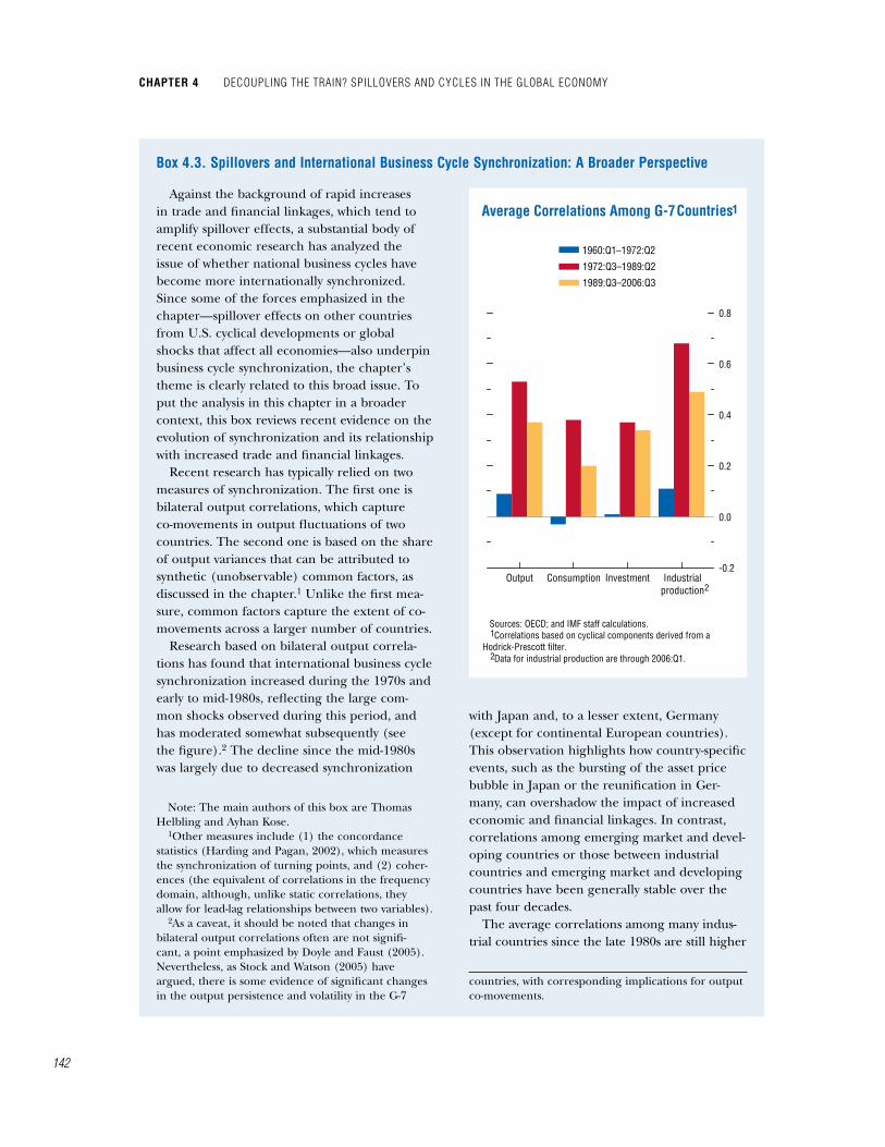
chapter 4 Decoupling the train? SpilloverS anD cycleS in the global economy
142
Against the background of rapid increases in trade and financial linkages, which tend to amplify spillover effects, a substantial body of recent economic research has analyzed the issue of whether national business cycles have become more internationally synchronized. Since some of the forces emphasized in the chapter—spillover effects on other countries from U.S. cyclical developments or global shocks that affect all economies—also underpin business cycle synchronization, the chapter’s theme is clearly related to this broad issue. To put the analysis in this chapter in a broader context, this box reviews recent evidence on the evolution of synchronization and its relationship with increased trade and financial linkages.
Recent research has typically relied on two measures of synchronization. The first one is bilateral output correlations, which capture co-movements in output fluctuations of two countries. The second one is based on the share of output variances that can be attributed to synthetic (unobservable) common factors, as discussed in the chapter.1 Unlike the first mea-sure, common factors capture the extent of co- movements across a larger number of countries.
Research based on bilateral output correla-tions has found that international business cycle synchronization increased during the 1970s and early to mid-1980s, reflecting the large com-mon shocks observed during this period, and has moderated somewhat subsequently (see the figure).2 The decline since the mid-1980s was largely due to decreased synchronization
Note: The main authors of this box are Thomas Helbling and Ayhan Kose.
1Other measures include (1) the concordance statistics (Harding and Pagan, 2002), which measures the synchronization of turning points, and (2) coher-ences (the equivalent of correlations in the frequency domain, although, unlike static correlations, they allow for lead-lag relationships between two variables).
2As a caveat, it should be noted that changes in bilateral output correlations often are not signifi-cant, a point emphasized by Doyle and Faust (2005). Nevertheless, as Stock and Watson (2005) have argued, there is some evidence of significant changes in the output persistence and volatility in the G-7
with Japan and, to a lesser extent, Germany (except for continental European countries). This observation highlights how country-specific events, such as the bursting of the asset price bubble in Japan or the reunification in Ger-many, can overshadow the impact of increased economic and financial linkages. In contrast, correlations among emerging market and devel-oping countries or those between industrial countries and emerging market and developing countries have been generally stable over the past four decades.
The average correlations among many indus-trial countries since the late 1980s are still higher
countries, with corresponding implications for output co-movements.
box 4.3. Spillovers and international business cycle Synchronization: a broader perspective
Sources: OECD; and IMF staff calculations. Correlations based on cyclical components derived from a Hodrick-Prescott filter. Data for industrial production are through 2006:Q1.
1
1960:Q1–1972:Q2
1972:Q3–1989:Q2
-0.2
0.0
0.2
0.4
0.6
0.8
Average Correlations Among G-7 Countries1
Output Consumption Investment Industrial production
1989:Q3–2006:Q3
2
2
Box 4.3
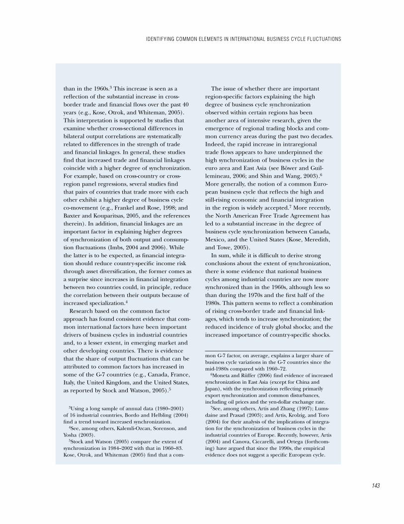
than in the 1960s.3 This increase is seen as a reflection of the substantial increase in cross-border trade and financial flows over the past 40 years (e.g., Kose, Otrok, and Whiteman, 2005). This interpretation is supported by studies that examine whether cross-sectional differences in bilateral output correlations are systematically related to differences in the strength of trade and financial linkages. In general, these studies find that increased trade and financial linkages coincide with a higher degree of synchronization. For example, based on cross-country or cross-region panel regressions, several studies find that pairs of countries that trade more with each other exhibit a higher degree of business cycle co-movement (e.g., Frankel and Rose, 1998; and Baxter and Kouparitsas, 2005, and the references therein). In addition, financial linkages are an important factor in explaining higher degrees of synchronization of both output and consump-tion fluctuations (Imbs, 2004 and 2006). While the latter is to be expected, as financial integra-tion should reduce country-specific income risk through asset diversification, the former comes as a surprise since increases in financial integration between two countries could, in principle, reduce the correlation between their outputs because of increased specialization.4
Research based on the common factor approach has found consistent evidence that com-mon international factors have been important drivers of business cycles in industrial countries and, to a lesser extent, in emerging market and other developing countries. There is evidence that the share of output fluctuations that can be attributed to common factors has increased in some of the G-7 countries (e.g., Canada, France, Italy, the United Kingdom, and the United States, as reported by Stock and Watson, 2005).5
3Using a long sample of annual data (1980–2001) of 16 industrial countries, Bordo and Helbling (2004) find a trend toward increased synchronization.
4See, among others, Kalemli-Ozcan, Sorenson, and Yosha (2003).
5Stock and Watson (2005) compare the extent of synchronization in 1984–2002 with that in 1960–83. Kose, Otrok, and Whiteman (2005) find that a com-
The issue of whether there are important region-specific factors explaining the high degree of business cycle synchronization observed within certain regions has been another area of intensive research, given the emergence of regional trading blocks and com-mon currency areas during the past two decades. Indeed, the rapid increase in intraregional trade flows appears to have underpinned the high synchronization of business cycles in the euro area and East Asia (see Böwer and Guil-lemineau, 2006; and Shin and Wang, 2003).6 More generally, the notion of a common Euro-pean business cycle that reflects the high and still-rising economic and financial integration in the region is widely accepted.7 More recently, the North American Free Trade Agreement has led to a substantial increase in the degree of business cycle synchronization between Canada, Mexico, and the United States (Kose, Meredith, and Towe, 2005).
In sum, while it is difficult to derive strong conclusions about the extent of synchronization, there is some evidence that national business cycles among industrial countries are now more synchronized than in the 1960s, although less so than during the 1970s and the first half of the 1980s. This pattern seems to reflect a combination of rising cross-border trade and financial link-ages, which tends to increase synchronization; the reduced incidence of truly global shocks; and the increased importance of country-specific shocks.
mon G-7 factor, on average, explains a larger share of business cycle variations in the G-7 countries since the mid-1980s compared with 1960–72.
6Moneta and Rüffer (2006) find evidence of increased synchronization in East Asia (except for China and Japan), with the synchronization reflecting primarily export synchronization and common disturbances, including oil prices and the yen-dollar exchange rate.
7See, among others, Artis and Zhang (1997); Lums-daine and Prasad (2003); and Artis, Krolzig, and Toro (2004) for their analysis of the implications of integra-tion for the synchronization of business cycles in the industrial countries of Europe. Recently, however, Artis (2004) and Canova, Ciccarelli, and Ortega (forthcom-ing) have argued that since the 1990s, the empirical evidence does not suggest a specific European cycle.
iDentiFying common elementS in international buSineSS cycle FluctuationS
143
chapter 4 Decoupling the train? SpilloverS anD cycleS in the global economy
144
concurrent cyclical fluctuations than common disturbances.24
how the united States affects the global economy—a model-based Simulation analysis
The analysis so far has shown that interna-tional spillover effects have been moderate on average. This average, however, hides a con-siderable diversity of experiences, with very large spillovers in some periods. There are two possible reasons for this. First, the extent of spillovers depends not only on the overall magnitudes of the underlying disturbances but also on their nature because this determines the relative importance of the various transmission channels. And, second, the transmission chan-nels themselves may have changed over time, in part because the conduct of monetary policy has changed considerably in recent decades. For a fuller assessment of the potential spillovers from the current U.S. slowdown, it is thus useful to complement the earlier analysis with simulation results based on a structural model. Specifically, this section traces the likely global effects of a U.S. demand disturbance using simulations of the IMF’s Global Economy Model (GEM), and attempts to isolate the factors that are likely to affect the size of spillovers.
GEM incorporates many trade linkages with an explicit microeconomic foundation and is thus well suited to analyze the effects of shocks that primarily involve the propagation through trade-related channels.25 It also provides the basis to analyze how such shocks can affect the nexus of interest rates, exchange rates, and monetary policy. GEM divides the world into several regions, which also allows for the analysis of how responses differ across regions. The simulations were conducted with a new five-
24Another possibility is that regional integration is more likely to lead to more common disturbances (or correlated disturbances because of similar developments in macroeconomic policies) at the regional level.
25See Laxton and Pesenti (2003) and Faruqee and oth-ers (2005) for details on the basic structure of GEM.
block version of GEM that involves the following countries/currency areas and regions: (1) the United States; (2) the euro area; (3) Japan; (4) emerging Asia; and (5) the remaining coun-tries. Each region is assumed to have flexible exchange rates, and to follow “inflation target-ing,” specifically, a forward-looking policy rule for nominal interest rates that targets expected inflation.26 The simulations are illustrative and should not be interpreted as forecasts.
Demand Shocks and trade linkages
A first simulation explores the impact of a “pure” country-specific shock to U.S. private demand. In the United States, this results in a slowdown in growth below the long-run trend for about two years, the lowest point of the contraction being reached after six quarters with a 1.4 percent decline in GDP compared with the baseline (Figure 4.8, first two rows). The reduc-tion in domestic demand leads to a more than proportional fall in import demand, reflecting the high import content in the cyclically sensi-tive parts of domestic demand noted earlier. As a result, the ratio of U.S. current account to GDP improves by almost 1 percentage point.
Lower U.S. import demand is the source of trade-related spillover effects, as it reduces final demand outside the United States. But com-pared with the decline in output in the United States, these effects are relatively small (Figure 4.8, lower two rows). This primarily reflects the small share in GDP of exports to the United States in all regions. The differences in the output responses across regions mirror the differences in their trade exposure to the U.S. economy (see Table 4.2).
26Technically, the monetary reaction function in GEM is an inflation-forecast-based (IFB) rule in which interest rates are adjusted in response to the forecast of inflation three quarters ahead. The weight on expected inflation has been calibrated to bring the forecast of inflation gradually back to the target and in a way that is cognizant of the implications for the real economy (see Laxton and Pesenti, 2003, for a discussion of IFB rules and the related literature).
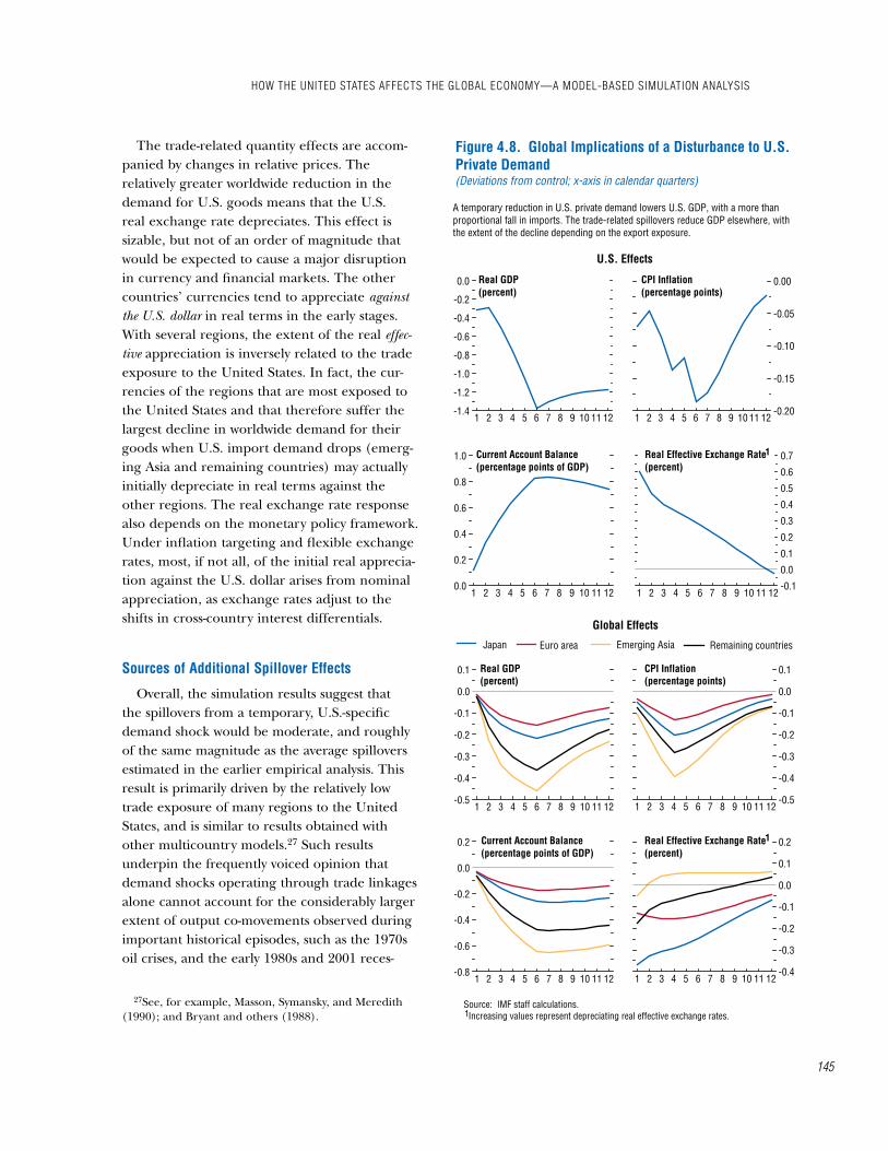
The trade-related quantity effects are accom-panied by changes in relative prices. The relatively greater worldwide reduction in the demand for U.S. goods means that the U.S. real exchange rate depreciates. This effect is sizable, but not of an order of magnitude that would be expected to cause a major disruption in currency and financial markets. The other countries’ currencies tend to appreciate against the U.S. dollar in real terms in the early stages. With several regions, the extent of the real effec-tive appreciation is inversely related to the trade exposure to the United States. In fact, the cur-rencies of the regions that are most exposed to the United States and that therefore suffer the largest decline in worldwide demand for their goods when U.S. import demand drops (emerg-ing Asia and remaining countries) may actually initially depreciate in real terms against the other regions. The real exchange rate response also depends on the monetary policy framework. Under inflation targeting and flexible exchange rates, most, if not all, of the initial real apprecia-tion against the U.S. dollar arises from nominal appreciation, as exchange rates adjust to the shifts in cross-country interest differentials.
Sources of additional Spillover effects
Overall, the simulation results suggest that the spillovers from a temporary, U.S.-specific demand shock would be moderate, and roughly of the same magnitude as the average spillovers estimated in the earlier empirical analysis. This result is primarily driven by the relatively low trade exposure of many regions to the United States, and is similar to results obtained with other multicountry models.27 Such results underpin the frequently voiced opinion that demand shocks operating through trade linkages alone cannot account for the considerably larger extent of output co-movements observed during important historical episodes, such as the 1970s oil crises, and the early 1980s and 2001 reces-
27See, for example, Masson, Symansky, and Meredith (1990); and Bryant and others (1988).
Source: IMF staff calculations. Increasing values represent depreciating real effective exchange rates.
Figure 4.8. Global Implications of a Disturbance to U.S. Private Demand(Deviations from control; x-axis in calendar quarters)
A temporary reduction in U.S. private demand lowers U.S. GDP, with a more than proportional fall in imports. The trade-related spillovers reduce GDP elsewhere, with the extent of the decline depending on the export exposure.
1 2 3 4 5 6 7 8 9 10 11 12-1.4
-1.2
-1.0
-0.8
-0.6
-0.4
-0.2
0.0
Real GDP(percent)
1 2 3 4 5 6 7 8 9 10 11 120.0
0.2
0.4
0.6
0.8
1.0
Real GDP(percent)
1 2 3 4 5 6 7 8 9 10 11 12-0.20
-0.15
-0.10
-0.05
0.00CPI Inflation(percentage points)
Current Account Balance(percentage points of GDP)
1 2 3 4 5 6 7 8 9 10 11 12-0.1
0.0
0.1
0.2
0.3
0.4
0.5
0.6
0.7Real Effective Exchange Rate(percent)
1 2 3 4 5 6 7 8 9 10 11 12-0.5
-0.4
-0.3
-0.2
-0.1
0.0
0.1
1 2 3 4 5 6 7 8 9 10 11 12-0.5
-0.4
-0.3
-0.2
-0.1
0.0
0.1CPI Inflation(percentage points)
Current Account Balance(percentage points of GDP)
1 2 3 4 5 6 7 8 9 10 11 12-0.8
-0.6
-0.4
-0.2
0.0
0.2
U.S. Effects
1 2 3 4 5 6 7 8 9 10 11 12-0.4
-0.3
-0.2
-0.1
0.0
0.1
0.2Real Effective Exchange Rate(percent)
Global Effects
Euro areaJapan Remaining countriesEmerging Asia
1
1
1
how the uniteD StateS aFFectS the global economy—a moDel-baSeD Simulation analySiS
145
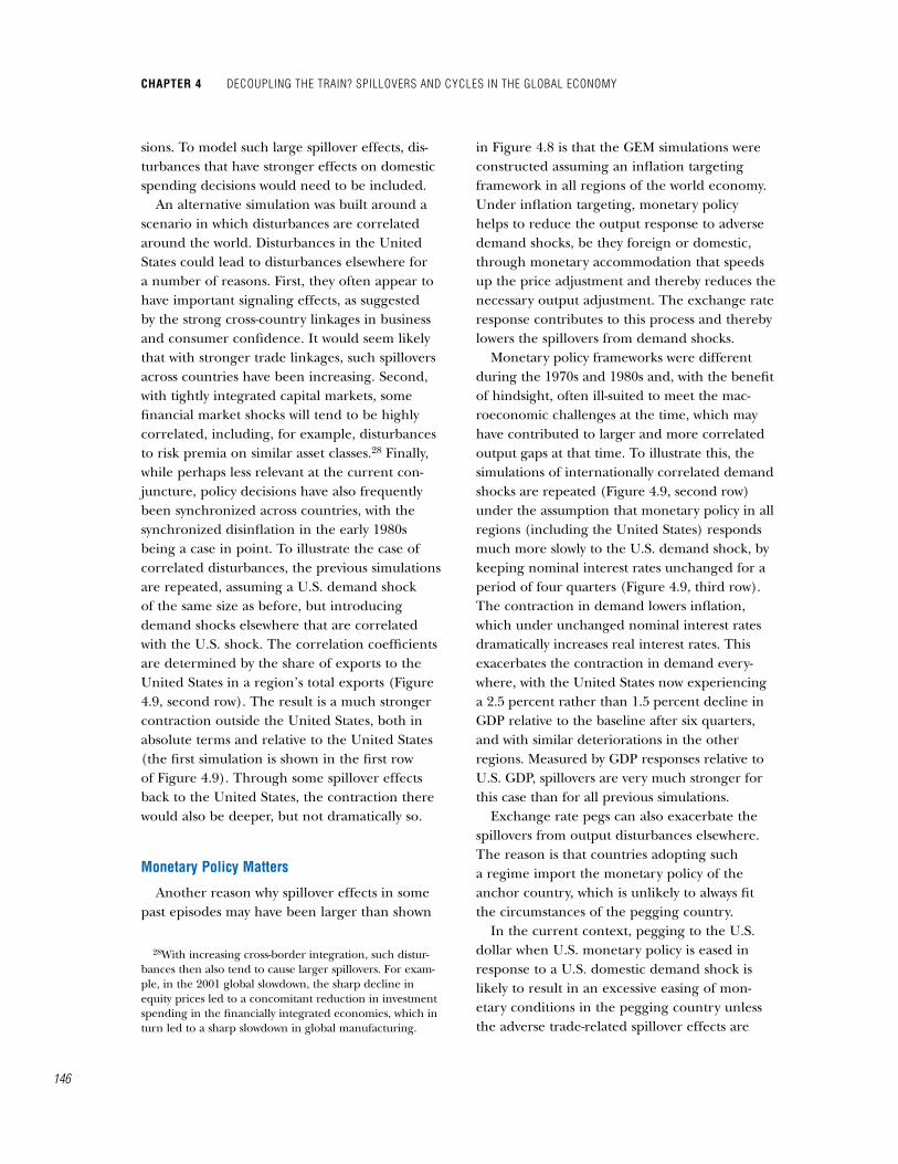
chapter 4 Decoupling the train? SpilloverS anD cycleS in the global economy
146
sions. To model such large spillover effects, dis-turbances that have stronger effects on domestic spending decisions would need to be included.
An alternative simulation was built around a scenario in which disturbances are correlated around the world. Disturbances in the United States could lead to disturbances elsewhere for a number of reasons. First, they often appear to have important signaling effects, as suggested by the strong cross-country linkages in business and consumer confidence. It would seem likely that with stronger trade linkages, such spillovers across countries have been increasing. Second, with tightly integrated capital markets, some financial market shocks will tend to be highly correlated, including, for example, disturbances to risk premia on similar asset classes.28 Finally, while perhaps less relevant at the current con-juncture, policy decisions have also frequently been synchronized across countries, with the synchronized disinflation in the early 1980s being a case in point. To illustrate the case of correlated disturbances, the previous simulations are repeated, assuming a U.S. demand shock of the same size as before, but introducing demand shocks elsewhere that are correlated with the U.S. shock. The correlation coefficients are determined by the share of exports to the United States in a region’s total exports (Figure 4.9, second row). The result is a much stronger contraction outside the United States, both in absolute terms and relative to the United States (the first simulation is shown in the first row of Figure 4.9). Through some spillover effects back to the United States, the contraction there would also be deeper, but not dramatically so.
monetary policy matters
Another reason why spillover effects in some past episodes may have been larger than shown
28With increasing cross-border integration, such distur-bances then also tend to cause larger spillovers. For exam-ple, in the 2001 global slowdown, the sharp decline in equity prices led to a concomitant reduction in investment spending in the financially integrated economies, which in turn led to a sharp slowdown in global manufacturing.
in Figure 4.8 is that the GEM simulations were constructed assuming an inflation targeting framework in all regions of the world economy. Under inflation targeting, monetary policy helps to reduce the output response to adverse demand shocks, be they foreign or domestic, through monetary accommodation that speeds up the price adjustment and thereby reduces the necessary output adjustment. The exchange rate response contributes to this process and thereby lowers the spillovers from demand shocks.
Monetary policy frameworks were different during the 1970s and 1980s and, with the benefit of hindsight, often ill-suited to meet the mac-roeconomic challenges at the time, which may have contributed to larger and more correlated output gaps at that time. To illustrate this, the simulations of internationally correlated demand shocks are repeated (Figure 4.9, second row) under the assumption that monetary policy in all regions (including the United States) responds much more slowly to the U.S. demand shock, by keeping nominal interest rates unchanged for a period of four quarters (Figure 4.9, third row). The contraction in demand lowers inflation, which under unchanged nominal interest rates dramatically increases real interest rates. This exacerbates the contraction in demand every-where, with the United States now experiencing a 2.5 percent rather than 1.5 percent decline in GDP relative to the baseline after six quarters, and with similar deteriorations in the other regions. Measured by GDP responses relative to U.S. GDP, spillovers are very much stronger for this case than for all previous simulations.
Exchange rate pegs can also exacerbate the spillovers from output disturbances elsewhere. The reason is that countries adopting such a regime import the monetary policy of the anchor country, which is unlikely to always fit the circumstances of the pegging country.
In the current context, pegging to the U.S. dollar when U.S. monetary policy is eased in response to a U.S. domestic demand shock is likely to result in an excessive easing of mon-etary conditions in the pegging country unless the adverse trade-related spillover effects are

very strong. With excessive monetary policy eas-ing, output in the pegging country would rise initially, given the fall in the real interest rate and the real exchange rate, but decrease subse-quently (below its medium-term path) as higher inflation would lead to an appreciation of the real exchange rate. In the case of stronger trade spillovers, however, the easing of monetary conditions implied by the peg for the particular disturbance at hand may be closer to the easing implied by an inflation targeting rule.29
The preceding arguments illustrate the fun-damental point that forward-looking monetary policy rules coupled with exchange rate flexibil-ity help to reduce the output effects of adverse demand shocks in many situations. In this sense, the GEM simulations reflect the major changes in macroeconomic policy frameworks that have occurred during the past decade. From a global perspective, it is worth emphasizing that mon-etary policy frameworks that are geared toward domestic price stability can also contribute to reducing fluctuations in world growth.
Summary and conclusionsThis chapter has analyzed how the U.S. econ-
omy affects international business cycle fluctua-tions, with a view to identifying the factors that influence the extent of U.S. spillovers into other countries. The analysis suggests that the limited global impact of the current U.S. slowdown so far is not surprising since the slowdown has been driven by U.S.-specific developments—primarily in housing and manufacturing—rather than by broader factors that are highly correlated across the major industrial countries.
Given the characteristics of the U.S. slowdown to date, the transmission to other countries operates primarily through demand channels, that is, through the effects on other countries’
29This explains why, for the type of disturbances explored in this section, the choice of monetary policy rule makes less of a difference for the case of emerging Asia than it would for some of the other regions. For sim-plicity, the simulations therefore assume the same policy rule in all regions.
1 2 3 4 5 6 7 8 9 10 11 12-3.0
-2.5
-2.0
-1.5
-1.0
-0.5
0.0
Figure 4.9. Global Growth and Inflation with Correlated Disturbances and Delayed Monetary Policy Response(Deviations from control; x-axis in calendar quarters)
Disturbances to U.S. private demand that are associated with disturbances elsewhere have a much larger impact on global growth. The slowing in growth is exacerbated if the monetary policy response is not appropriately forward looking.
1 2 3 4 5 6 7 8 9 10 11 12-1.4
-1.2
-1.0
-0.8
-0.6
-0.4
-0.2
0.0
0.2
Delayed Interest Rate Responses: GDP(percent)
1 2 3 4 5 6 7 8 9 10 11 12-2.0
-1.5
-1.0
-0.5
0.0
1 2 3 4 5 6 7 8 9 10 11 12-0.25
-0.20
-0.15
-0.10
-0.05
0.00
0.05U.S. Disturbance Only: GDP(percent)
U.S. Disturbance Only: Inflation(percentage points)
Correlated Disturbances: GDP(percent)
1 2 3 4 5 6 7 8 9 10 11 12-0.5
-0.4
-0.3
-0.2
-0.1
0.0Correlated Disturbances: Inflation(percentage points)
1 2 3 4 5 6 7 8 9 10 11 12-1.4
-1.2
-1.0
-0.8
-0.6
-0.4
-0.2
0.0Delayed Interest Rate Responses: Inflation(percentage points)
United StatesWorld World excluding U.S.
Source: IMF staff calculations. See simulation results in Figure 4.8.1
11
Summary anD concluSionS
147
chapter 4 Decoupling the train? SpilloverS anD cycleS in the global economy
148
exports to the United States, which, by them-selves, tend to be modest. In this respect, the fact that the import content in the housing sec-tor is relatively small has helped to mitigate the spillover effects on other countries. In contrast, if the transmission had also involved asset price spillovers or confidence channels, the impact would likely have been larger.
Overall, these factors suggest that most countries should be in a position to “decouple” from the U.S. economy and sustain strong growth if the U.S. slowdown remains as moderate as expected, although countries with strong trade linkages with the United States in specific sec-tors may experience some drag on their growth. However, if the U.S. economy experienced a sharper slowdown because of a broader-than-expected impact of the housing sector difficul-ties, the spillover effects into other economies would be larger, and decoupling would be more difficult. Nevertheless, with increasingly flex-ible macroeconomic policy frameworks in many countries, monetary policy should be well posi-tioned to cushion the potential contractionary effects on economic activity.
In addition to these conclusions about the global implications of the current slowdown, the chapter’s other main findings about the role of the U.S. economy in international business cycle fluctuations are as follows.• The old saying, “If the United States sneezes,
the rest of the world catches a cold,” remains relevant since the analysis shows that reces-sions in the United States (and, to a lesser extent, in other large economies) can exert significant spillovers on both advanced and developing economies. However, it also is an exaggeration because the estimated spill-overs, as measured by the declines in output growth, are generally considerably smaller than the output decrease in the United States itself, particularly in the context of midcycle slowdowns.
• The influence of the U.S. economy on other economies does not appear to have dimin-ished. On the contrary, indications are that the magnitudes of spillovers have increased
over time, particularly in neighboring coun-tries and regions, which is consistent with the notion that greater trade and financial integration tends to magnify the cross-border effects of disturbances.
• More generally, the analysis highlights that past episodes with large synchronized declines in global growth were characterized by com-mon disturbances that were either truly global in nature (e.g., abrupt oil price changes), were correlated across countries (e.g., disin-flationary policies during the early 1980s), or involved global movements in asset prices (e.g., the synchronous equity price declines during 2000–01). In other words, past epi-sodes of highly synchronized growth declines were not primarily the result of spillovers as defined in this chapter, but of common (or correlated) disturbances.
• During the past two decades, common global factors have become somewhat less important drivers of national business cycle fluctuations. At the same time, the importance of regional factors among the highly integrated econo-mies in North America, western Europe, and emerging Asia appears to have increased. These contrasting developments reflect that global disturbances have become less fre-quent and smaller, while intraregional trade and financial linkages have, in general, risen more rapidly than extraregional ones. Overall, compared with the 1970s and early 1980s, the world economy may thus continue to see less synchronized international business cycles at the global level unless it is subjected to the common disturbances that were the hallmark of earlier episodes.
• Policy responses can moderate or amplify the spillover effects of disturbances in the United States (or other large economies). Forward-looking monetary policy responses in the context of an inflation targeting framework have tended to reduce the output response to adverse demand disturbances, be they foreign or domestic. In contrast, monetary policy responses that are not sufficiently forward looking or flexible risk magnifying
the spillover effects. To the extent that the strong international business cycle linkages in the early 1980s reflected the adjustment to disinflationary monetary policies, this episode may not prove relevant today.
appendix 4.1. econometric methodologyThe main author of this appendix is Nikola Spatafora.
This appendix provides details of the econo-metric methodology used to estimate the effects of disturbances in major economies on output and other variables elsewhere.
a broad cross-country analysis
The analysis in this subsection, based on panel growth regressions, most closely resembles Arora and Vamvakidis (2006). One crucial difference is that it is carried out using annual data, rather than five-year averages; the approach here seems more relevant to the shorter-run business cycle spillovers that are the focus of this chapter. The focus of this analysis is similar to that of other studies that have analyzed the determinants of cross-country output correlations, though it adopts a different methodology from theirs.30
In the panel regressions, the dependent vari-able is growth in domestic output per capita, measured in PPP-adjusted dollars; this variable is drawn from the Penn World Tables. The inde-pendent variables include the following:• growth in U.S., euro area, and Japanese
output per capita, measured in PPP-adjusted dollars (source: Penn World Tables);
• trade linkages with the United States, the euro area, and Japan; as defined in the text (source: IMF, Direction of Trade Statistics);
• financial linkages with the United States, the euro area, and Japan. In addition to the measure defined in the text, two alternative measures were created: (1) a country’s total Gross Foreign Assets plus total Gross For-
30Including, for instance, Calderón, Chong, and Stein (2007); and Imbs (2004 and 2006).
eign Liabilities, as a ratio to GDP; and (2) a country’s gross holdings of U.S., euro area, or Japanese assets, as appropriate, plus its gross liabilities to U.S., euro area, or Japanese residents, again as a ratio to GDP. The second measure, drawn from the Coordinated Port-folio Investment Survey of portfolio assets, is only available for 1997, 2001, 2003, and 2004. Neither of these two alternative measures proved significant;
• exchange rate regime. This was classi-fied as “fixed” if it corresponded, in the Reinhart-Rogoff (2004) classification, to a currency board; peg; crawling peg; band; pre-announced crawling band; or de facto crawling band narrower than or equal to +/– 2 percent. All other exchange rate regimes were classified as “floating.” On aver-age, over the full sample period, 66 countries (including 61 developing countries) were deemed to have fixed exchange rates; 43 countries (including 37 developing countries) were deemed to have floating exchange rates;
• public sector debt stock; public sector deficit. Debt stocks were classified as “large” if they exceeded 40 percent of GDP, and “small” oth-erwise. For deficits, the threshold was set at 3 percent of GDP. In both cases, the threshold roughly corresponds to the sample mean;
• initial GDP; population growth (source: Penn World Tables);
• the (log) change in the terms of trade; the six-month LIBOR (source: World Economic Outlook database); and
• indicators denoting the Latin American debt crisis of 1982, the Latin American Tequila cri-ses of 1995, the East Asian crises of 1997–98, and the Argentine crisis of 2002.31
All estimates are based on the Arellano-Bond fixed effects estimator. For comparison, Arora and Vamvakidis (2006) find much larger
31To the extent that these crises themselves reflected a spillover from developments in advanced economies, any procedure that controls separately for their impact will understate the true magnitude of spillovers. However, none of the estimates presented are in fact sensitive to excluding the crisis indicators.
appenDix 4.1. econometric methoDology
149
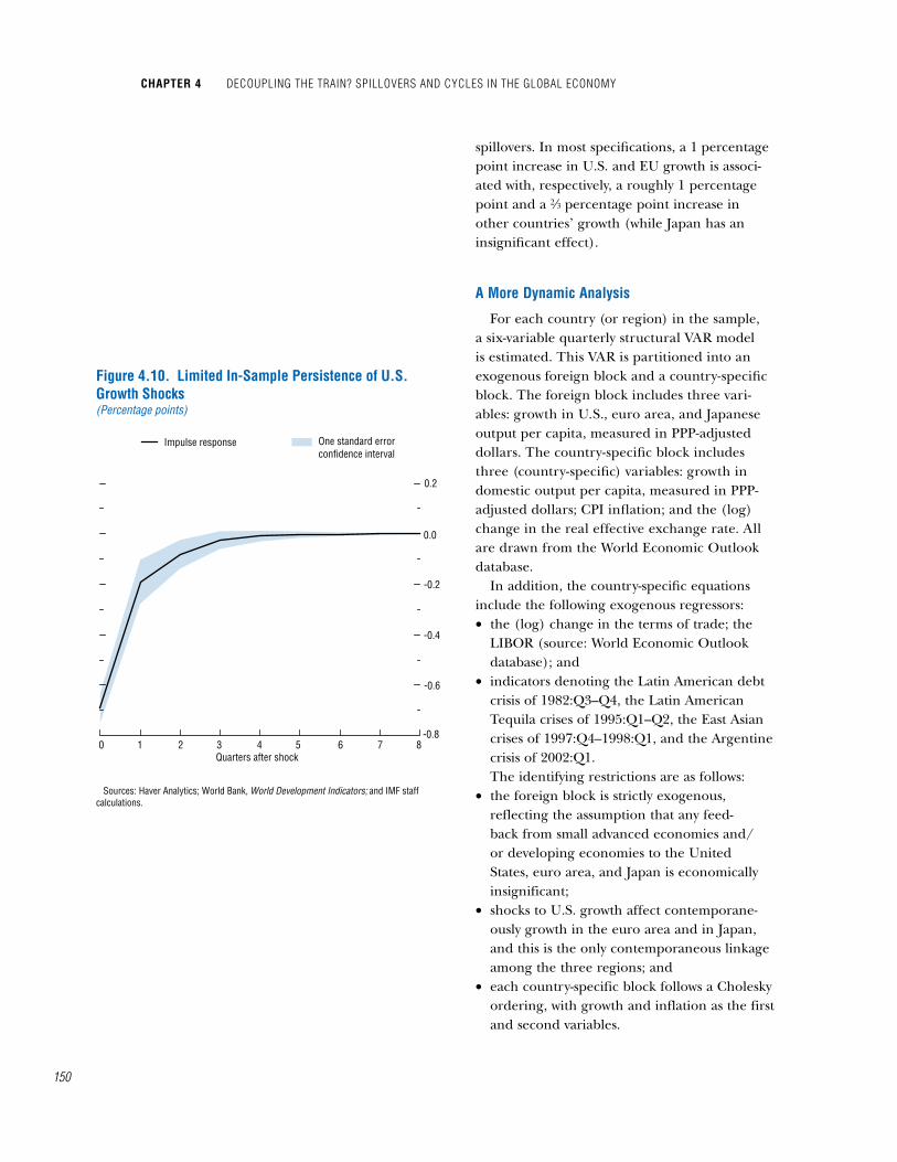
chapter 4 Decoupling the train? SpilloverS anD cycleS in the global economy
150
spillovers. In most specifications, a 1 percentage point increase in U.S. and EU growth is associ-ated with, respectively, a roughly 1 percentage point and a @/3 percentage point increase in other countries’ growth (while Japan has an insignificant effect).
a more Dynamic analysis
For each country (or region) in the sample, a six-variable quarterly structural VAR model is estimated. This VAR is partitioned into an exogenous foreign block and a country-specific block. The foreign block includes three vari-ables: growth in U.S., euro area, and Japanese output per capita, measured in PPP-adjusted dollars. The country-specific block includes three (country-specific) variables: growth in domestic output per capita, measured in PPP-adjusted dollars; CPI inflation; and the (log) change in the real effective exchange rate. All are drawn from the World Economic Outlook database.
In addition, the country-specific equations include the following exogenous regressors:• the (log) change in the terms of trade; the
LIBOR (source: World Economic Outlook database); and
• indicators denoting the Latin American debt crisis of 1982:Q3–Q4, the Latin American Tequila crises of 1995:Q1–Q2, the East Asian crises of 1997:Q4–1998:Q1, and the Argentine crisis of 2002:Q1.The identifying restrictions are as follows:
• the foreign block is strictly exogenous, reflecting the assumption that any feed-back from small advanced economies and/or developing economies to the United States, euro area, and Japan is economically insignificant;
• shocks to U.S. growth affect contemporane-ously growth in the euro area and in Japan, and this is the only contemporaneous linkage among the three regions; and
• each country-specific block follows a Cholesky ordering, with growth and inflation as the first and second variables.
Figure 4.10. Limited In-Sample Persistence of U.S. Growth Shocks(Percentage points)
Sources: Haver Analytics; World Bank, World Development Indicators; and IMF staff calculations.
-0.6
-0.8
Quarters after shock
-0.4
-0.2
0.0
0.2
One standard error confidence interval
Impulse response
0 1 2 3 4 5 6 7 8
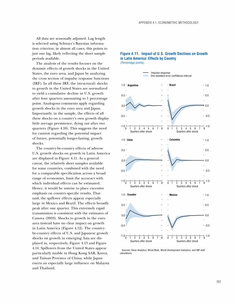
All data are seasonally adjusted. Lag length is selected using Schwarz’s Bayesian informa-tion criterion; in almost all cases, this points to just one lag, likely reflecting the short sample periods available.
The analysis of the results focuses on the dynamic effects of growth shocks in the United States, the euro area, and Japan by analyzing the cross section of impulse response functions (IRF). In all these IRF, the (structural) shocks to growth in the United States are normalized to yield a cumulative decline in U.S. growth after four quarters amounting to 1 percentage point. Analogous comments apply regarding growth shocks in the euro area and Japan. Importantly, in the sample, the effects of all these shocks on a country’s own growth display little average persistence, dying out after two quarters (Figure 4.10). This suggests the need for caution regarding the potential impact of future, potentially longer-lasting, growth shocks.
The country-by-country effects of adverse U.S. growth shocks on growth in Latin America are displayed in Figure 4.11. As a general caveat, the relatively short samples available for some countries, combined with the need for a comparable specification across a broad range of economies, limit the accuracy with which individual effects can be estimated. Hence, it would be unwise to place excessive emphasis on country-specific results. That said, the spillover effects appear especially large in Mexico and Brazil. The effects broadly peak after one quarter. This extremely rapid transmission is consistent with the estimates of Canova (2003). Shocks to growth in the euro area instead have no clear impact on growth in Latin America (Figure 4.12). The country-by-country effects of U.S. and Japanese growth shocks on growth in emerging Asia are dis-played in, respectively, Figure 4.13 and Figure 4.14. Spillovers from the United States appear particularly sizable in Hong Kong SAR, Korea, and Taiwan Province of China, while Japan exerts an especially large influence on Malaysia and Thailand.
Figure 4.11. Impact of U.S. Growth Declines on Growthin Latin America: Effects by Country(Percentage points)
Impulse response One standard error confidence interval
Argentina
-0.5
0.0
0.5
1.0 Brazil
-0.5
0.0
0.5
1.0
-0.5
0.0
0.5
1.0
-0.5
0.0
0.5
1.0Chile Colombia
-0.5
0.0
0.5
1.0
-0.5
0.0
0.5
1.0Ecuador Mexico
Quarters after shock
-1.0
Quarters after shock
-1.00 1 2 3 4 5 6 7 8 0 1 2 3 4 5 6 7 8
Quarters after shock
-1.0
Quarters after shock
-1.00 1 2 3 4 5 6 7 8 0 1 2 3 4 5 6 7 8
Quarters after shock
-1.0
Quarters after shock
-1.00 1 2 3 4 5 6 7 8 0 1 2 3 4 5 6 7 8
Sources: Haver Analytics; World Bank, World Development Indicators; and IMF staff calculations.
appenDix 4.1. econometric methoDology
151
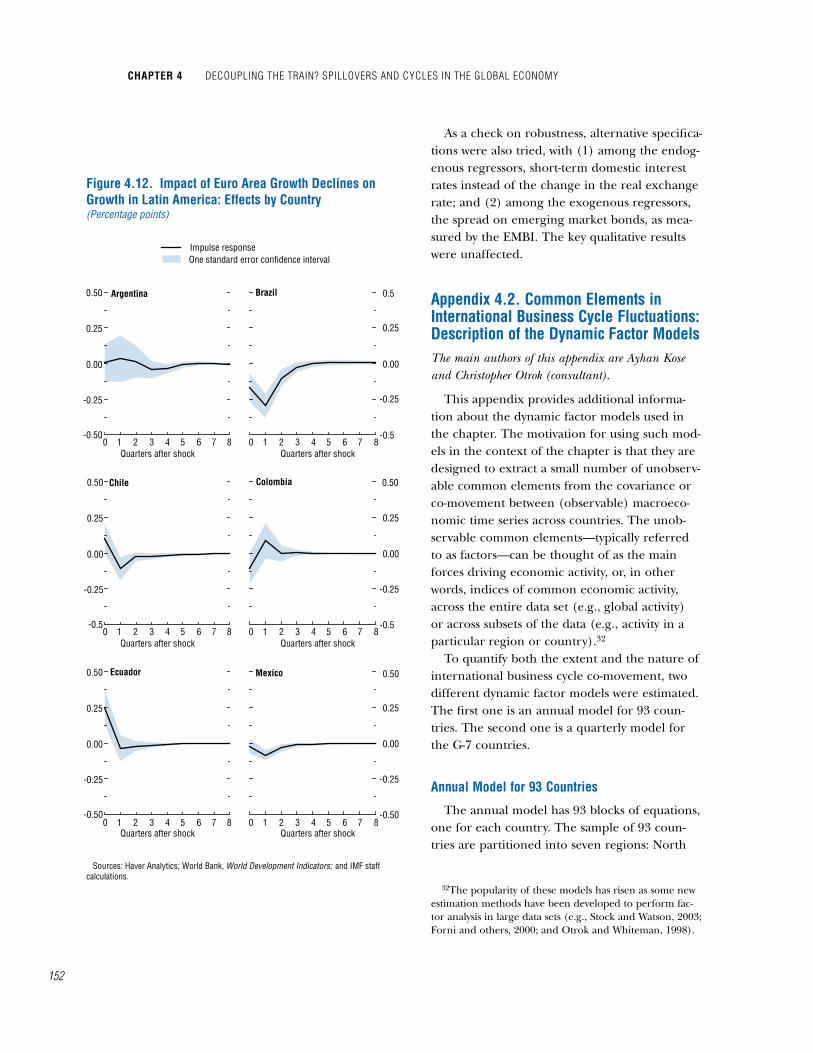
chapter 4 Decoupling the train? SpilloverS anD cycleS in the global economy
152
As a check on robustness, alternative specifica-tions were also tried, with (1) among the endog-enous regressors, short-term domestic interest rates instead of the change in the real exchange rate; and (2) among the exogenous regressors, the spread on emerging market bonds, as mea-sured by the EMBI. The key qualitative results were unaffected.
appendix 4.2. common elements in international business cycle Fluctuations: Description of the Dynamic Factor modelsThe main authors of this appendix are Ayhan Kose and Christopher Otrok (consultant).
This appendix provides additional informa-tion about the dynamic factor models used in the chapter. The motivation for using such mod-els in the context of the chapter is that they are designed to extract a small number of unobserv-able common elements from the covariance or co-movement between (observable) macroeco-nomic time series across countries. The unob-servable common elements—typically referred to as factors—can be thought of as the main forces driving economic activity, or, in other words, indices of common economic activity, across the entire data set (e.g., global activity) or across subsets of the data (e.g., activity in a particular region or country).32
To quantify both the extent and the nature of international business cycle co-movement, two different dynamic factor models were estimated. The first one is an annual model for 93 coun-tries. The second one is a quarterly model for the G-7 countries.
annual model for 93 countries
The annual model has 93 blocks of equations, one for each country. The sample of 93 coun-tries are partitioned into seven regions: North
32The popularity of these models has risen as some new estimation methods have been developed to perform fac-tor analysis in large data sets (e.g., Stock and Watson, 2003; Forni and others, 2000; and Otrok and Whiteman, 1998).
Figure 4.12. Impact of Euro Area Growth Declines on Growth in Latin America: Effects by Country(Percentage points)
Impulse response One standard error confidence interval
Argentina
-0.25
0.00
0.25
0.50 Brazil
-0.25
0.00
0.25
0.5
-0.25
0.00
0.25
0.50
-0.25
0.00
0.25
0.50Chile Colombia
-0.25
0.00
0.25
0.50
-0.25
0.00
0.25
0.50Ecuador Mexico
Quarters after shock
-0.50
Quarters after shock
-0.500 1 2 3 4 5 6 7 8 0 1 2 3 4 5 6 7 8
Quarters after shock
-0.5
Quarters after shock
-0.50 1 2 3 4 5 6 7 8 0 1 2 3 4 5 6 7 8
Quarters after shock
-0.50
Quarters after shock
-0.50 1 2 3 4 5 6 7 8 0 1 2 3 4 5 6 7 8
Sources: Haver Analytics; World Bank, World Development Indicators; and IMF staff calculations.
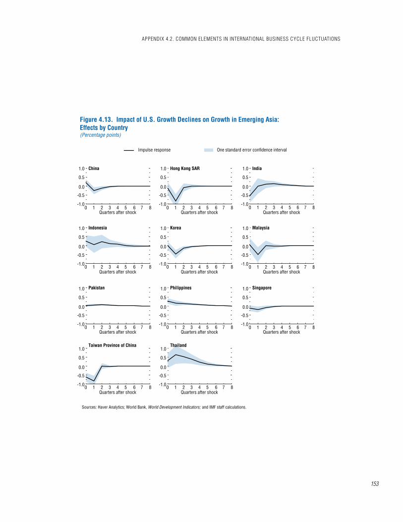
Figure 4.13. Impact of U.S. Growth Declines on Growth in Emerging Asia: Effects by Country(Percentage points)
Impulse response One standard error confidence interval
China
-0.5
0.0
0.5
1.0 Hong Kong SAR India
-0.5
0.0
0.5
1.0
-0.5
0.0
0.5
1.0
Indonesia Korea Malaysia
-0.5
0.0
0.5
1.0
-0.5
0.0
0.5
1.0
-0.5
0.0
0.5
1.0
Pakistan Philippines Singapore
-0.5
0.0
0.5
1.0
-0.5
0.0
0.5
1.0
-0.5
0.0
0.5
1.0
Taiwan Province of China Thailand
-0.5
0.0
0.5
1.0
-0.5
0.0
0.5
1.0
Sources: Haver Analytics; World Bank, World Development Indicators; and IMF staff calculations.
Quarters after shock Quarters after shock
-1.0 -1.00 1 2 3 4 5 6 7 8 0 1 2 3 4 5 6 7 8
Quarters after shock Quarters after shock Quarters after shock
-1.0 -1.0 -1.00 1 2 3 4 5 6 7 8 0 1 2 3 4 5 6 7 8 0 1 2 3 4 5 6 7 8
Quarters after shock Quarters after shock Quarters after shock
-1.0 -1.0 -1.00 1 2 3 4 5 6 7 8 0 1 2 3 4 5 6 7 8 0 1 2 3 4 5 6 7 8
Quarters after shock
-1.0
Quarters after shock Quarters after shock
-1.0 -1.00 1 2 3 4 5 6 7 8 0 1 2 3 4 5 6 7 8 0 1 2 3 4 5 6 7 8
appenDix 4.2. common elementS in international buSineSS cycle FluctuationS
153
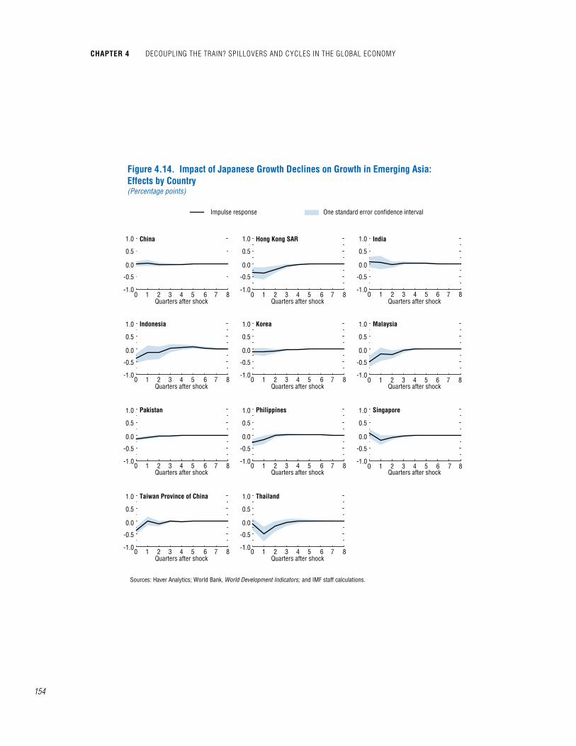
chapter 4 Decoupling the train? SpilloverS anD cycleS in the global economy
154
Figure 4.14. Impact of Japanese Growth Declines on Growth in Emerging Asia: Effects by Country(Percentage points)
China
Quarters after shock
-0.5
-1.0
0.0
0.5
1.0
Impulse response One standard error confidence interval
Hong Kong SAR
Quarters after shock
India
Quarters after shock
Indonesia
Quarters after shock
Korea
Quarters after shock
Malaysia
Quarters after shock
Pakistan
Quarters after shock
Philippines
Quarters after shock
Singapore
Quarters after shock
-0.5
-1.0
0.0
0.5
1.0
-0.5
-1.0
0.0
0.5
1.0
Taiwan Province of China
Quarters after shock
Thailand
Quarters after shock
-0.5
-1.0
0.0
0.5
1.0
-0.5
-1.0
0.0
0.5
1.0
-0.5
-1.0
0.0
0.5
1.0
-0.5
-1.0
0.0
0.5
1.0
-0.5
-1.0
0.0
0.5
1.0
-0.5
-1.0
0.0
0.5
1.0
-0.5
-1.0
0.0
0.5
1.0
-0.5
-1.0
0.0
0.5
1.0
0 1 2 3 4 5 6 7 8 0 1 2 3 4 5 6 7 8 0 1 2 3 4 5 6 7 8
0 1 2 3 4 5 6 7 8 0 1 2 3 4 5 6 7 8 0 1 2 3 4 5 6 7 8
0 1 2 3 4 5 6 7 8 0 1 2 3 4 5 6 7 8 0 1 2 3 4 5 6 7 8
0 1 2 3 4 5 6 7 8 0 1 2 3 4 5 6 7 8
Sources: Haver Analytics; World Bank, World Development Indicators; and IMF staff calculations.
America, Western Europe, Oceania, Asia, Latin America, Middle East and North Africa, and sub-Saharan Africa. The grouping of countries by region is useful in identifing a “regional factor” because countries that are geographi-cally close to each other are likely to be directly affected by some regional shocks, including, for example, weather-related shocks. Each country block contains three equations, one for output growth (Y ), one for private consumption growth (C ), and one for growth of private fixed invest-ment (I ). Each equation decomposes growth in Y, C, or I into a global factor, a regional factor, a country-specific factor, and a residual (idiosyn-cratic) component. For example, the block of equations for the first country, the United States (US ), in the first region, North America (NA), is
YUS,t = bUSY,G ft
Global + bUSY,NA ft
NA + bUSY ft
US + cYUS,t,
CUS,t = bUSC,G ft
Global + bUSC,NA ft
NA + bUSC ft
US + cCUS,t,
IUS,t = bUSI,G ft
Global + bUSI,NA ft
NA + bUSI ft
US + cIUS,t.
The same block of equations is repeated for each country in the seven regions in the system.
The global factor is the component common to all countries in this system. The sensitivity of output growth in each country j in the system to the global factor depends on bj
Y,G, the factor loading. There is also a regional factor, which captures co-movement across the countries in a region.
The model captures dynamic co-movement by allowing the factors and the series-specific terms (the c terms in the above equations) to be (independent) autoregressive processes. That is, each factor or country-specific term depends on lags of itself and an independent and identically distributed innovation to the variable (ut). For example, for the global factor, the autoregressive processes are
ftGlobal = φ(L)ft–1
Global + utGlobal,
where φ(L) is a lag polynomial and ut is normally distributed. All of the factor loadings (b coef-ficients in the first set of equations) and the lag polynomials are independent of each other. The model is estimated using Bayesian techniques as
described in Kose, Otrok, and Whiteman (2003) and Otrok, Silos, and Whiteman (2003).33
To measure the importance of each factor, so-called variance decompositions that decompose the total volatility of output growth into volatility components due to each factor are calculated. The formula for the variance decomposition is derived by applying the variance operator to each equation in the system. For example, for the first equation,
var(YUS) = (bUSY,G )2 var(f Global) + (bUS
Y,NA)2 var(f NA) + (bUS
Y )2 var(f US) + var(cYUS).
There are no cross-product terms between the factors because they are orthogonal to each other. The variance in real per capita output growth attributable to the global factor then follows as
(bUSGlobal)2 var(f Global)
––––––––––––––––. var(YUS)
The model was estimated for the period 1960–2005 and for two subperiods, 1960–1985 and 1986–2005.
The list of countries included in the estima-tion is as follows (by region): • North America: United States and Canada;• Oceania: Australia and New Zealand;• Western Europe: United Kingdom, Austria,
Belgium, Denmark, France, Germany, Italy, Luxembourg, Netherlands, Norway, Sweden, Switzerland, Finland, Greece, Iceland, Ireland, Portugal, and Spain; and
• Latin America: Argentina, Bolivia, Brazil, Chile, Colombia, Costa Rica, Dominican Republic, Ecuador, El Salvador, Guatemala, Honduras, Mexico, Nicaragua, Panama, Para-guay, Peru, Uruguay, and Venezuela.
33The innovation variance of the factors (error term in the factor autoregressive equation) is normalized. This normalization is based on the variance of the underly-ing series and determines the scale of the factor (0.1 versus 0.01). This dependency on scaling is the reason for looking only at variance decompositions or appropriately scaled versions of the factors (factor times factor loading, as in the computation of variance shown below). The model is estimated using de-meaned output growth data allowing for a break in 1986.
appenDix 4.2. common elementS in international buSineSS cycle FluctuationS
155
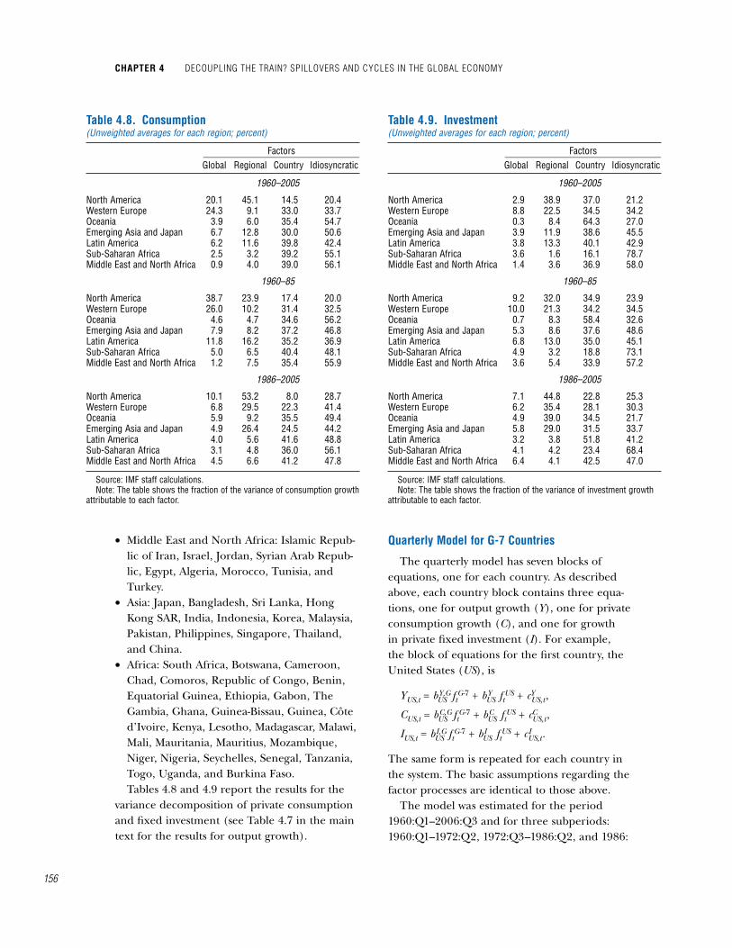
chapter 4 Decoupling the train? SpilloverS anD cycleS in the global economy
156
• Middle East and North Africa: Islamic Repub-lic of Iran, Israel, Jordan, Syrian Arab Repub-lic, Egypt, Algeria, Morocco, Tunisia, and Turkey.
• Asia: Japan, Bangladesh, Sri Lanka, Hong Kong SAR, India, Indonesia, Korea, Malaysia, Pakistan, Philippines, Singapore, Thailand, and China.
• Africa: South Africa, Botswana, Cameroon, Chad, Comoros, Republic of Congo, Benin, Equatorial Guinea, Ethiopia, Gabon, The Gambia, Ghana, Guinea-Bissau, Guinea, Côte d’Ivoire, Kenya, Lesotho, Madagascar, Malawi, Mali, Mauritania, Mauritius, Mozambique, Niger, Nigeria, Seychelles, Senegal, Tanzania, Togo, Uganda, and Burkina Faso.Tables 4.8 and 4.9 report the results for the
variance decomposition of private consumption and fixed investment (see Table 4.7 in the main text for the results for output growth).
Quarterly model for g-7 countries
The quarterly model has seven blocks of equations, one for each country. As described above, each country block contains three equa-tions, one for output growth (Y), one for private consumption growth (C), and one for growth in private fixed investment (I). For example, the block of equations for the first country, the United States (US), is
YUS,t = bUSY,G ft
G-7 + bUSY ft
US + cYUS,t,
CUS,t = bUSC,G ft
G-7 + bUSC ft
US + cCUS,t,
IUS,t = bUSI,G ft
G-7 + bUSI ft
US + cIUS,t.
The same form is repeated for each country in the system. The basic assumptions regarding the factor processes are identical to those above.
The model was estimated for the period 1960:Q1–2006:Q3 and for three subperiods: 1960:Q1–1972:Q2, 1972:Q3–1986:Q2, and 1986:
table 4.8. consumption(Unweighted averages for each region; percent)
Factors _________________________________ Global Regional Country Idiosyncratic
1960–2005
North America 20.1 45.1 14.5 20.4Western Europe 24.3 9.1 33.0 33.7Oceania 3.9 6.0 35.4 54.7Emerging Asia and Japan 6.7 12.8 30.0 50.6Latin America 6.2 11.6 39.8 42.4Sub-Saharan Africa 2.5 3.2 39.2 55.1Middle East and North Africa 0.9 4.0 39.0 56.1
1960–85
North America 38.7 23.9 17.4 20.0Western Europe 26.0 10.2 31.4 32.5Oceania 4.6 4.7 34.6 56.2Emerging Asia and Japan 7.9 8.2 37.2 46.8Latin America 11.8 16.2 35.2 36.9Sub-Saharan Africa 5.0 6.5 40.4 48.1Middle East and North Africa 1.2 7.5 35.4 55.9
1986–2005
North America 10.1 53.2 8.0 28.7Western Europe 6.8 29.5 22.3 41.4Oceania 5.9 9.2 35.5 49.4Emerging Asia and Japan 4.9 26.4 24.5 44.2Latin America 4.0 5.6 41.6 48.8Sub-Saharan Africa 3.1 4.8 36.0 56.1Middle East and North Africa 4.5 6.6 41.2 47.8
Source: IMF staff calculations.Note: The table shows the fraction of the variance of consumption growth
attributable to each factor.
table 4.9. investment(Unweighted averages for each region; percent)
Factors _________________________________ Global Regional Country Idiosyncratic
1960–2005
North America 2.9 38.9 37.0 21.2Western Europe 8.8 22.5 34.5 34.2Oceania 0.3 8.4 64.3 27.0Emerging Asia and Japan 3.9 11.9 38.6 45.5Latin America 3.8 13.3 40.1 42.9Sub-Saharan Africa 3.6 1.6 16.1 78.7Middle East and North Africa 1.4 3.6 36.9 58.0
1960–85
North America 9.2 32.0 34.9 23.9Western Europe 10.0 21.3 34.2 34.5Oceania 0.7 8.3 58.4 32.6Emerging Asia and Japan 5.3 8.6 37.6 48.6Latin America 6.8 13.0 35.0 45.1Sub-Saharan Africa 4.9 3.2 18.8 73.1Middle East and North Africa 3.6 5.4 33.9 57.2
1986–2005
North America 7.1 44.8 22.8 25.3Western Europe 6.2 35.4 28.1 30.3Oceania 4.9 39.0 34.5 21.7Emerging Asia and Japan 5.8 29.0 31.5 33.7Latin America 3.2 3.8 51.8 41.2Sub-Saharan Africa 4.1 4.2 23.4 68.4Middle East and North Africa 6.4 4.1 42.5 47.0
Source: IMF staff calculations.Note: The table shows the fraction of the variance of investment growth
attributable to each factor.
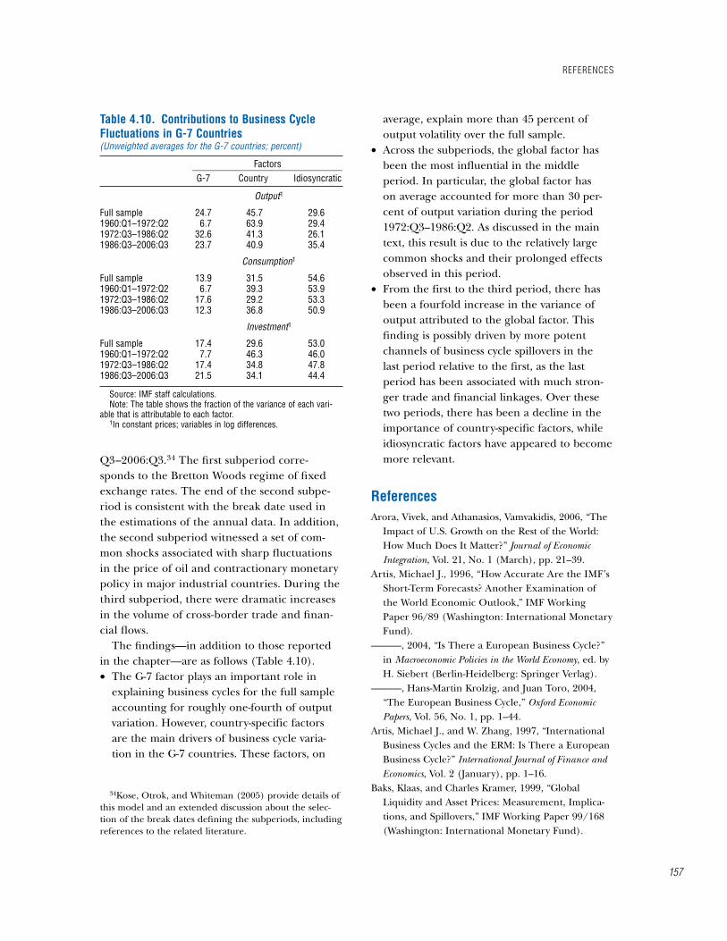
Q3–2006:Q3.34 The first subperiod corre-sponds to the Bretton Woods regime of fixed exchange rates. The end of the second subpe-riod is consistent with the break date used in the estimations of the annual data. In addition, the second subperiod witnessed a set of com-mon shocks associated with sharp fluctuations in the price of oil and contractionary monetary policy in major industrial countries. During the third subperiod, there were dramatic increases in the volume of cross-border trade and finan-cial flows.
The findings—in addition to those reported in the chapter—are as follows (Table 4.10).• The G-7 factor plays an important role in
explaining business cycles for the full sample accounting for roughly one-fourth of output variation. However, country-specific factors are the main drivers of business cycle varia-tion in the G-7 countries. These factors, on
34Kose, Otrok, and Whiteman (2005) provide details of this model and an extended discussion about the selec-tion of the break dates defining the subperiods, including references to the related literature.
average, explain more than 45 percent of output volatility over the full sample.
• Across the subperiods, the global factor has been the most influential in the middle period. In particular, the global factor has on average accounted for more than 30 per-cent of output variation during the period 1972:Q3–1986:Q2. As discussed in the main text, this result is due to the relatively large common shocks and their prolonged effects observed in this period.
• From the first to the third period, there has been a fourfold increase in the variance of output attributed to the global factor. This finding is possibly driven by more potent channels of business cycle spillovers in the last period relative to the first, as the last period has been associated with much stron-ger trade and financial linkages. Over these two periods, there has been a decline in the importance of country-specific factors, while idiosyncratic factors have appeared to become more relevant.
referencesArora, Vivek, and Athanasios, Vamvakidis, 2006, “The
Impact of U.S. Growth on the Rest of the World: How Much Does It Matter?” Journal of Economic Integration, Vol. 21, No. 1 (March), pp. 21–39.
Artis, Michael J., 1996, “How Accurate Are the IMF’s Short-Term Forecasts? Another Examination of the World Economic Outlook,” IMF Working Paper 96/89 (Washington: International Monetary Fund).
———, 2004, “Is There a European Business Cycle?” in Macroeconomic Policies in the World Economy, ed. by H. Siebert (Berlin-Heidelberg: Springer Verlag).
———, Hans-Martin Krolzig, and Juan Toro, 2004, “The European Business Cycle,” Oxford Economic Papers, Vol. 56, No. 1, pp. 1–44.
Artis, Michael J., and W. Zhang, 1997, “International Business Cycles and the ERM: Is There a European Business Cycle?” International Journal of Finance and Economics, Vol. 2 (January), pp. 1–16.
Baks, Klaas, and Charles Kramer, 1999, “Global Liquidity and Asset Prices: Measurement, Implica-tions, and Spillovers,” IMF Working Paper 99/168 (Washington: International Monetary Fund).
table 4.10. contributions to business cycle Fluctuations in g-7 countries(Unweighted averages for the G-7 countries; percent)
Factors ________________________________ G-7 Country Idiosyncratic
Output1
Full sample 24.7 45.7 29.61960:Q1–1972:Q2 6.7 63.9 29.41972:Q3–1986:Q2 32.6 41.3 26.11986:Q3–2006:Q3 23.7 40.9 35.4
Consumption1
Full sample 13.9 31.5 54.61960:Q1–1972:Q2 6.7 39.3 53.91972:Q3–1986:Q2 17.6 29.2 53.31986:Q3–2006:Q3 12.3 36.8 50.9
Investment1
Full sample 17.4 29.6 53.01960:Q1–1972:Q2 7.7 46.3 46.01972:Q3–1986:Q2 17.4 34.8 47.81986:Q3–2006:Q3 21.5 34.1 44.4
Source: IMF staff calculations.Note: The table shows the fraction of the variance of each vari-
able that is attributable to each factor.1In constant prices; variables in log differences.
reFerenceS
157
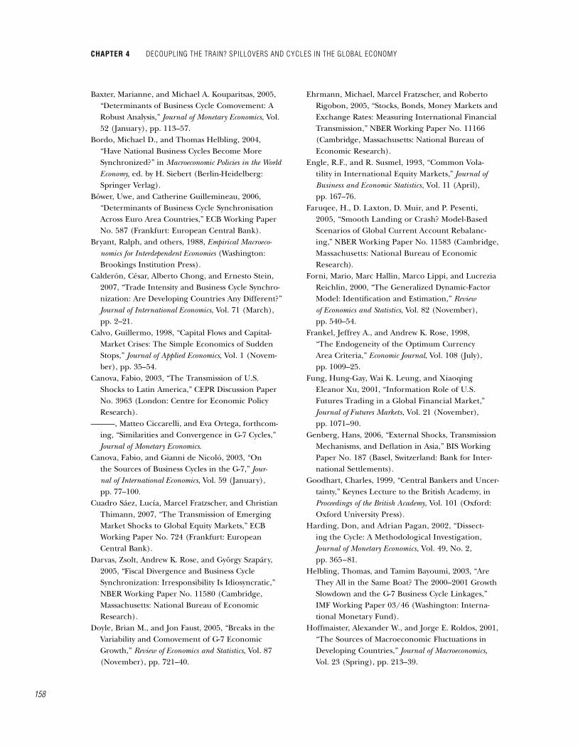
chapter 4 Decoupling the train? SpilloverS anD cycleS in the global economy
158
Baxter, Marianne, and Michael A. Kouparitsas, 2005, “Determinants of Business Cycle Comovement: A Robust Analysis,” Journal of Monetary Economics, Vol. 52 (January), pp. 113–57.
Bordo, Michael D., and Thomas Helbling, 2004, “Have National Business Cycles Become More Synchronized?” in Macroeconomic Policies in the World Economy, ed. by H. Siebert (Berlin-Heidelberg: Springer Verlag).
Böwer, Uwe, and Catherine Guillemineau, 2006, “Determinants of Business Cycle Synchronisation Across Euro Area Countries,” ECB Working Paper No. 587 (Frankfurt: European Central Bank).
Bryant, Ralph, and others, 1988, Empirical Macroeco-nomics for Interdependent Economies (Washington: Brookings Institution Press).
Calderón, César, Alberto Chong, and Ernesto Stein, 2007, “Trade Intensity and Business Cycle Synchro-nization: Are Developing Countries Any Different?” Journal of International Economics, Vol. 71 (March), pp. 2–21.
Calvo, Guillermo, 1998, “Capital Flows and Capital-Market Crises: The Simple Economics of Sudden Stops,” Journal of Applied Economics, Vol. 1 (Novem-ber), pp. 35–54.
Canova, Fabio, 2003, “The Transmission of U.S. Shocks to Latin America,” CEPR Discussion Paper No. 3963 (London: Centre for Economic Policy Research).
———, Matteo Ciccarelli, and Eva Ortega, forthcom-ing, “Similarities and Convergence in G-7 Cycles,” Journal of Monetary Economics.
Canova, Fabio, and Gianni de Nicoló, 2003, “On the Sources of Business Cycles in the G-7,” Jour-nal of International Economics, Vol. 59 (January), pp. 77–100.
Cuadro Sáez, Lucía, Marcel Fratzscher, and Christian Thimann, 2007, “The Transmission of Emerging Market Shocks to Global Equity Markets,” ECB Working Paper No. 724 (Frankfurt: European Central Bank).
Darvas, Zsolt, Andrew K. Rose, and György Szapáry, 2005, “Fiscal Divergence and Business Cycle Synchronization: Irresponsibility Is Idiosyncratic,” NBER Working Paper No. 11580 (Cambridge, Massachusetts: National Bureau of Economic Research).
Doyle, Brian M., and Jon Faust, 2005, “Breaks in the Variability and Comovement of G-7 Economic Growth,” Review of Economics and Statistics, Vol. 87 (November), pp. 721–40.
Ehrmann, Michael, Marcel Fratzscher, and Roberto Rigobon, 2005, “Stocks, Bonds, Money Markets and Exchange Rates: Measuring International Financial Transmission,” NBER Working Paper No. 11166 (Cambridge, Massachusetts: National Bureau of Economic Research).
Engle, R.F., and R. Susmel, 1993, “Common Vola-tility in International Equity Markets,” Journal of Business and Economic Statistics, Vol. 11 (April), pp. 167–76.
Faruqee, H., D. Laxton, D. Muir, and P. Pesenti, 2005, “Smooth Landing or Crash? Model-Based Scenarios of Global Current Account Rebalanc-ing,” NBER Working Paper No. 11583 (Cambridge, Massachusetts: National Bureau of Economic Research).
Forni, Mario, Marc Hallin, Marco Lippi, and Lucrezia Reichlin, 2000, “The Generalized Dynamic-Factor Model: Identification and Estimation,” Review of Economics and Statistics, Vol. 82 (November), pp. 540–54.
Frankel, Jeffrey A., and Andrew K. Rose, 1998, “The Endogeneity of the Optimum Currency Area Criteria,” Economic Journal, Vol. 108 (July), pp. 1009–25.
Fung, Hung-Gay, Wai K. Leung, and Xiaoqing Eleanor Xu, 2001, “Information Role of U.S. Futures Trading in a Global Financial Market,” Journal of Futures Markets, Vol. 21 (November), pp. 1071–90.
Genberg, Hans, 2006, “External Shocks, Transmission Mechanisms, and Deflation in Asia,” BIS Working Paper No. 187 (Basel, Switzerland: Bank for Inter-national Settlements).
Goodhart, Charles, 1999, “Central Bankers and Uncer-tainty,” Keynes Lecture to the British Academy, in Proceedings of the British Academy, Vol. 101 (Oxford: Oxford University Press).
Harding, Don, and Adrian Pagan, 2002, “Dissect-ing the Cycle: A Methodological Investigation, Journal of Monetary Economics, Vol. 49, No. 2, pp. 365–81.
Helbling, Thomas, and Tamim Bayoumi, 2003, “Are They All in the Same Boat? The 2000–2001 Growth Slowdown and the G-7 Business Cycle Linkages,” IMF Working Paper 03/46 (Washington: Interna-tional Monetary Fund).
Hoffmaister, Alexander W., and Jorge E. Roldos, 2001, “The Sources of Macroeconomic Fluctuations in Developing Countries,” Journal of Macroeconomics, Vol. 23 (Spring), pp. 213–39.
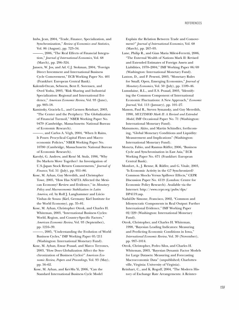
Imbs, Jean, 2004, “Trade, Finance, Specialization, and Synchronization,” Review of Economics and Statistics, Vol. 86 (August), pp. 723–34.
———, 2006, “The Real Effects of Financial Integra-tion,” Journal of International Economics, Vol. 68 (March), pp. 296–324.
Jansen, W. Jos, and Ad. C.J. Stokman, 2004, “Foreign Direct Investment and International Business Cycle Comovement,” ECB Working Paper No. 401 (Frankfurt: European Central Bank).
Kalemli-Ozcan, Sebnem, Bent E. Sorensen, and Oved Yosha, 2003, “Risk Sharing and Industrial Specialization: Regional and International Evi-dence,” American Economic Review, Vol. 93 (June), pp. 903–18.
Kaminsky, Graciela L., and Carmen Reinhart, 2003, “The Center and the Periphery: The Globalization of Financial Turmoil,” NBER Working Paper No. 9479 (Cambridge, Massachusetts: National Bureau of Economic Research).
———, and Carlos A. Végh, 2004, “When It Rains, It Pours: Procyclical Capital Flows and Macro-economic Policies,” NBER Working Paper No. 10780 (Cambridge, Massachusetts: National Bureau of Economic Research).
Karolyi, G. Andrew, and René M. Stulz, 1996, “Why Do Markets Move Together? An Investigation of U.S.-Japan Stock Return Comovements,” Journal of Finance, Vol. 51 (July), pp. 951–86.
Kose, M. Ayhan, Guy Meredith, and Christopher Towe, 2005, “How Has NAFTA Affected the Mexi-can Economy? Review and Evidence,” in Monetary Policy and Macroeconomic Stabilization in Latin America, ed. by Rolf J. Langhammer and Lúcio Vinhas de Souza (Kiel, Germany: Kiel Institute for the World Economy), pp. 35–81.
Kose, M. Ayhan, Christopher Otrok, and Charles H. Whiteman, 2003, “International Business Cycles: World, Region, and Country-Specific Factors,” American Economic Review, Vol. 93 (September), pp. 1216–39.
———, 2005, “Understanding the Evolution of World Business Cycles,” IMF Working Paper 05/211 (Washington: International Monetary Fund).
Kose, M. Ayhan, Eswar Prasad, and Marco Terrones, 2003, “How Does Globalization Affect the Syn-chronization of Business Cycles?” American Eco-nomic Review, Papers and Proceedings, Vol. 93 (May), pp. 56–62.
Kose, M. Ayhan, and Kei-Mu Yi, 2006, “Can the Standard International Business Cycle Model
Explain the Relation Between Trade and Comove-ment?” Journal of International Economics, Vol. 68 (March), pp. 267–95.
Lane, Philip R., and Gian Maria Milesi-Ferretti, 2006, “The External Wealth of Nations Mark II: Revised and Extended Estimates of Foreign Assets and Liabilities, 1970–2004,” IMF Working Paper 06/69 (Washington: International Monetary Fund).
Laxton, D., and P. Pesenti, 2003, “Monetary Rules for Small, Open, Emerging Economies,” Journal of Monetary Economics, Vol. 50 (July), pp. 1109–46.
Lumsdaine, R.L., and E.S. Prasad, 2003, “Identify-ing the Common Component of International Economic Fluctuations: A New Approach,” Economic Journal, Vol. 113 (January), pp. 101–27.
Masson, Paul R., Steven Symansky, and Guy Meredith, 1990, MULTIMOD Mark II: A Revised and Extended Model, IMF Occasional Paper No. 71 (Washington: International Monetary Fund).
Matsumoto, Akito, and Martin Schindler, forthcom-ing, “Global Monetary Conditions and Liquidity: Measurement and Implications” (Washington: International Monetary Fund).
Moneta, Fabio, and Rasmus Rüffer, 2006, “Business Cycle and Synchronisation in East Asia,” ECB Working Paper No. 671 (Frankfurt: European Central Bank).
Monfort, A., J. Renne, R. Rüffer, and G. Vitale, 2003, “Is Economic Activity in the G7 Synchronized? Common Shocks Versus Spillover Effects,” CEPR Discussion Paper No. 4119 (London: Centre for Economic Policy Research). Available via the Internet: http://www.cepr.org/pubs/dps/ DP4119.asp.
Nadal-De Simone, Francisco, 2002, “Common and Idiosyncratic Components in Real Output: Further International Evidence,” IMF Working Paper 02/229 (Washington: International Monetary Fund).
Otrok, Christopher, and Charles H. Whiteman, 1998, “Bayesian Leading Indicators: Measuring and Predicting Economic Conditions in Iowa,” International Economic Review, Vol. 39 (November), pp. 997–1014.
Otrok, Christopher, Pedro Silos, and Charles H. Whiteman, 2003, “Bayesian Dynamic Factor Models for Large Datasets: Measuring and Forecasting Macroeconomic Data” (unpublished; Charlottes-ville, Virginia: University of Virginia).
Reinhart, C., and K. Rogoff, 2004, “The Modern His-tory of Exchange Rate Arrangements: A Reinter-
reFerenceS
159
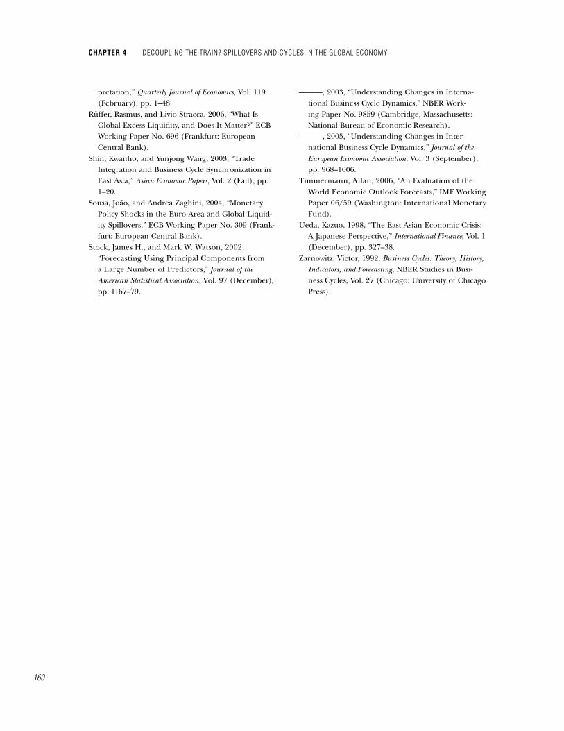
chapter 4 Decoupling the train? SpilloverS anD cycleS in the global economy
160
pretation,” Quarterly Journal of Economics, Vol. 119 (February), pp. 1–48.
Rüffer, Rasmus, and Livio Stracca, 2006, “What Is Global Excess Liquidity, and Does It Matter?” ECB Working Paper No. 696 (Frankfurt: European Central Bank).
Shin, Kwanho, and Yunjong Wang, 2003, “Trade Integration and Business Cycle Synchronization in East Asia,” Asian Economic Papers, Vol. 2 (Fall), pp. 1–20.
Sousa, João, and Andrea Zaghini, 2004, “Monetary Policy Shocks in the Euro Area and Global Liquid-ity Spillovers,” ECB Working Paper No. 309 (Frank-furt: European Central Bank).
Stock, James H., and Mark W. Watson, 2002, “Forecasting Using Principal Components from a Large Number of Predictors,” Journal of the American Statistical Association, Vol. 97 (December), pp. 1167–79.
———, 2003, “Understanding Changes in Interna-tional Business Cycle Dynamics,” NBER Work-ing Paper No. 9859 (Cambridge, Massachusetts: National Bureau of Economic Research).
———, 2005, “Understanding Changes in Inter-national Business Cycle Dynamics,” Journal of the European Economic Association, Vol. 3 (September), pp. 968–1006.
Timmermann, Allan, 2006, “An Evaluation of the World Economic Outlook Forecasts,” IMF Working Paper 06/59 (Washington: International Monetary Fund).
Ueda, Kazuo, 1998, “The East Asian Economic Crisis: A Japanese Perspective,” International Finance, Vol. 1 (December), pp. 327–38.
Zarnowitz, Victor, 1992, Business Cycles: Theory, History, Indicators, and Forecasting, NBER Studies in Busi-ness Cycles, Vol. 27 (Chicago: University of Chicago Press).