Deep Depth from Aberration Map

Masako Kashiwagi1 Nao Mishima1 Tatsuo Kozakaya1 Shinsaku Hiura2

1Toshiba Corporate Research & Development Center 2University of Hyogo

{firstname.lastname}@toshiba.co.jp hiura@eng.u-hyogo.ac.jp

Abstract

Passive and convenient depth estimation from single-

shot image is still an open problem. Existing depth from

defocus methods require multiple input images or special

hardware customization. Recent deep monocular depth es-

timation is also limited to an image with sufficient contex-

tual information. In this work, we propose a novel method

which realizes a single-shot deep depth measurement based

on physical depth cue using only an off-the-shelf camera

and lens. When a defocused image is taken by a camera,

it contains various types of aberrations corresponding to

distances from the image sensor and positions in the im-

age plane. We call these minute and complexly compound

aberrations as Aberration Map (A-Map) and we found that

A-Map can be utilized as reliable physical depth cue. Addi-

tionally, our deep network named A-Map Analysis Network

(AMA-Net) is also proposed, which can effectively learn and

estimate depth via A-Map. To evaluate the validity and ro-

bustness of our approach, we have conducted extensive ex-

periments using both real outdoor scenes and simulated im-

ages. The qualitative result shows the accuracy and avail-

ability of the method in comparison with a state-of-the-art

deep context-based method.

1. Introduction

Single-shot depth measurement using an off-the-shelf

camera is still an open problem despite remarkable ad-

vances in computational photography. In particular, the si-

multaneous pursuit of high robustness, low cost, and high

depth accuracy are challenging requirement for realizing

production.

For the single-shot approach, deep monocular depth es-

timation (DMDE) [17, 2] and depth from defocus (DfD)

[5, 14, 7, 19, 23, 25, 24] are mainly proposed in recent years.

DMDE is the most successful method, has greatly advanced

the accuracy of depth estimation by extracting contextual

information with a deep learning technique. Despite the re-

Single-shot image Depth map

FarNear

AMA-Net

Supervised learning

Aberration Map (A-Map)

Figure 1. Depth measurement from a single-shot image by super-

vised learning of Aberration Map (A-Map) which contains various

types of aberrations, position of image, and distance information.

markable progress of DMDE, it has a fundamental limita-

tion that a correct depth map cannot be estimated without

sufficient contextual information, for instance, in a scene

without the ground because it does not incorporate physical

depth cues. Conversely, single-shot DfD estimates depth

by purely simulating a model of defocus blur, without uti-

lizing contextual information. Although the depth cue is

physically given as defocus blur, the depth still has the near

side or far side ambiguity from the focal plane. While sev-

eral proposals which insert different types of color filters

[5, 7, 23, 25, 24] into the lens aperture solve this prob-

lem. Another approach of single-shot DfD focuses on axial

chromatic aberration [28, 9]. However, these approaches

need hardware customization to generate the desired aber-

ration. Moreover, it is difficult to model the actual point

spread functions (PSFs) because a camera lens generally

contains various types of aberration. Recently, a combina-

tion of DMDE and DfD named as deep depth from defocus

(DDfD) is proposed in [22]. Its main idea is to improve

4070

depth estimation by deep learning both defocus blur based

on DFD and contextual information. DDfD shows that out-

of-focus blur helps to improve the depth accuracy but it still

depends on contextual information and thus unavoidable the

inherent limitation of DMDE.

Since the actual aberrations are very minute and com-

plex in comparison with contextual information and defo-

cus blur, there has not been investigated yet how they affect

depth measurement, regarding to such both on-axis aberra-

tions and off-axis aberrations. Through our PSF measure-

ment experiment, we observed that actual defocused PSF

shapes produced by an off-the-shelf camera lens are unique

with respect to the distance from the image sensor and it

also has a position dependence in the image plane. We

call an image which contains this position-dependent and

distance-dependent aberrations as A-Map.

In this paper, we present a single-shot depth measure-

ment method using only an off-the-shelf camera. We

also propose A-Map Analysis Network (AMA-Net) which

learns the relationship between A-Map and corresponding

depth in a supervised manner. We demonstrate that our

method outperforms a conventional method in qualitative

evaluation, including various outdoor scenes. The main

contributions of this paper are listed below:

• We present a novel approach of physics-based single-

shot depth estimation by utilizing A-Map of an off-the-

shelf lens.

• We propose an original deep network, AMA-Net, which

consists of two branches, such as gradient brunch and

positional brunch, and efficiently estimates depth from

A-Map without involving contextual information.

• We demonstrated not only the robustness of our method

through qualitative and quantitative evaluations with

various outdoor textures, but also the validity of aber-

rations as depth cues by simulation studies.

2. Related work

One of the major methods for physics-based depth esti-

mation is depth from defocus (DfD). DfD is a passive depth

estimation based on modeling a defocus blur radius. A blur

radius b is derived from the lens-maker’s formula,

b =avf

2p|1

f−

1

u−

1

vf|, (1)

where u, a = fF

, f , F , p and vf are an object’s distance,

a diameter of the lens aperture, a focal length, an aperture

number, a sensor pitch and a distance between the lens and

the image sensor, respectively. Although the depth cue is

physically given as defocus blur, the depth still has the am-

biguity of near side or far side of the focal plane, because

there is same blur radius in both planes. Thus, DfD method

usually uses more than two-shot images to estimate the blur

radius [27].

For single-shot depth estimation with physical depth cue,

there are several proposals of color-coded apertures (CCA)

which insert different types of color filters [5, 14, 7, 19, 23,

25, 24] into a lens aperture. Another approach for generat-

ing depth cue in [28] is focusing on axial chromatic aberra-

tion (ACA) by using customized chromatic lens. Although

CCA and ACA can solve the depth ambiguity, they require

hardware customization to obtain sufficient physical depth

cue.

In recent years, deep learning approaches have greatly

advanced in computer vision, and there is no exception

for depth estimation. One of the successful methods is

DMDE [17, 2]. Generally, deep neural network is trained

with a large RGB-D dataset to learn variation of contex-

tual information. However, this method has limitation of

using images in the wild, for instance, in a scene without

the ground, sky or simple pattern such as a stripe.

The method of [22] combines DMDE with DfD to im-

prove depth estimation. They investigate that defocus blur

can be utilized as an additional depth cue. Although they

present great potential of blur information as physical depth

cues besides contextual information, it still depends on con-

textual information and is not yet detailed enough to analyze

blur information.

3. Method

The key point for accurate depth estimation is to find the

physical depth cues which should be unique within mea-

sured distances. To investigate various types of aberrations

can be utilized as a depth cue, first we describe lens aberra-

tion in Section 3.1 and then explain A-Map with measuring

and analyzing PSFs of an RGB camera lens in Section 3.2.

Finally, our deep network, A-Map analysis network (AMA-

Net) is proposed in Section 3.3.

3.1. Lens aberrations

Lens aberrations are generally categorized as chromatic

aberrations (CA) and monochromatic aberrations (MA). As

CA, there are two types such as axial chromatic aberrations

(ACA) and transverse chromatic aberrations (TCA). MA is

widely known as five Seidel aberrations: spherical aberra-

tions, coma, astigmatism, curvature of field and distortion.

In most cases, ACA and spherical aberrations occur at the

center of the image. On the other hand, TCA and coma

occur around the corner of the image. These types of aber-

rations depend on the angle of incidence (on or off axis) of

the light on the lens.

Some types of aberrations are illustrated in Figure 2. In

the case of single lens, each color, blue, green and red light

has different focal length due to dispersion (Figure 2 (a)).

When an object is in the far or near plane, blue or red

4071

(a) Single lens

In-Focus

Far

Near

(b) Achromatic lens

Image sensor

u vf

b

u vf

b

(e) Captured image

(c) Coma aberration

FarNear

(d) Actual coma PSF

Purple fringe (Near)

Green fringe (Far)

less blur (In-focus)

Figure 2. Various aberrations of actual lens. (a) ACA of single

lens, (b) ACA of achromatic lens, (c) Coma aberration, (d) Exam-

ple of actual coma PSF, and (e) Example of fringes produced by

actual camera lens aberrations.

fringe can be seen around the edge of captured images. Fig-

ure 2 (b) shows the simplest structure of achromatic lens

which typically corrects red and blue light. Nevertheless,

still purple and green fringes are observed in the near and far

plane since CA cannot be perfectly removed. Coma aberra-

tions are also difficult to remove and off-axis lights appear

as a comet-like tail on the image plane (Figure 2 (c) and (d)).

Even though a digital single-lens reflex camera (DSLR)

lens has a more complex structure with many lenses, the

colored-edge fringe is still visible (Figure 2 (e)).

3.2. Aberration Map

When considering the case of using product lens, blur

is produced from not only ACA but also other aberrations

which are hard to be suppressed perfectly. To investigate

the behavior of both on-axis and off-axis aberrations at the

same time, we first measure PSFs because various types of

aberrations are eventually expressed in the form of PSFs.

PSFs can be efficiently measured by using DSLR camera

and capturing an image of point light sources (a matrix of

white dots) which is displayed on high resolution display, at

various distances (details are described in Section 4.1). Fig-

ure 3 shows an example of measurement results, the mea-

(b) On-axis

In focusNear Far In focusNear Far

F4

(c) Off-axis

F1.8

x

x

(a) A-map (F1.8)

On-axis

Off-axis

In focusNear Far

Figure 3. PSF measurement results. The point light sources

were measured with f=50mm RGB-SDLR camera, F1.8 and F4,

at, near, in-focus, and far side, respectively. (a) is the example of

sampled A-Map F1.8. Pink and yellow square show on-axis and

off-axis PSF. (b) and (c) show expanded images of the on-axis and

off-axis where the position is squared in (a). The numerical val-

ues of the PSF in the horizontal direction (white arrow) are shown

below the expanded PSF images.

surement distance was 1000mm (near), 1500mm (in-focus)

and 2000mm (far). As the figure shows, PSF has a position

dependence of the image.

We named these images which show the distance and

position dependency of PSFs as A-Map.

Figure 3 (b) and (c) shows the results of on-axis and off-

axis with F1.8 and F4. In addition, the numerical values of

the PSF across horizontal direction are also shown. There

are two major differences between the near-plane and the

far-plane. The first one is the shape of the PSF, the over-

all rough shape is induced by defocusing, and the detailed

shape is induced by various aberrations. For example, the

near plane PSF forms a concave surface of the center por-

tion and the far plane forms a convex surface. The second

is the color fringe, the purple and green fringe is generated

by CA, observed at near and far, respectively. Furthermore,

the off-axis PSF’s shape (Figure 3) is different from on-axis

PSF, which is caused by off-axis aberrations such as TCA,

coma, and field curvature.

From the measurement results, it can be observed that the

shape of the PSFs of the defocused plane has corresponding

distance. In addition, it is clear that the PSF of the product’s

camera lens is too complicated to simulate, as the PSF is

generated from various kinds of aberrations. Therefore, the

4072

Glo

bal P

oolin

g

AB

U

Den

se

GT

i,ji,j

j i

Conv

Conv

Concat

Conv

ResB

lock

Max

poolin

g

××

Conv

ResB

lock

Max

poolin

g

Sigmoid

Conv

ResB

lock

Max

poolin

g

××

Conv

ResB

lock

Max

poolin

g

Sigmoid

Dep

th

Broadcast

Gradients

Position

Patch

Image

・・・

・・・

x4

x4

Positional branch

Gradient branch (Main)

Figure 4. The architecture of AMA-Net based on ResNet. A main

branch extracts blur from the gradients. A positional branch makes

attention maps. The main branch feature map is multiplied by the

attention maps.

Flat panel display

Natural image database

cameraAMA-Net

Image

(A-Map)

depth

12m Slide stage

140[inch]

Figure 5. Experimental system. The 12m automatic slide stage is

placed orthogonally to the display consisting of four 8K displays (to-

tal 140 inches, 15360 x 8640, 16K). RGB-DSLR camera is mounted

on the stage moving with 1mm accuracy.

deep learning method is considered to effectively analyze

complex A-Map.

3.3. AMA-Net

Archtecture. We developed A-Map analysis network

(AMA-Net) to analyze aberration blur efficiently. AMA-

Net architecture, shown in Figure 4, is based on

ResNet [10], and it has two branches: gradient branch

(main) and positional branch. Since A-Map contains var-

ious types of aberrations blur corresponding to position of

image and distance information, we adopt patch-based ar-

chitecture learning method [30, 26, 31, 21, 4, 3] to ana-

lyze only aberration blur. The architecture takes a patch

extracted from a captured image as an input, and then out-

puts a single depth value corresponding to the patch. This

network can be trained by patchwise images with flat depth

data only. Such data can be collected easily by our experi-

mental system (described in Section 4.1).

In the gradient branch as a main branch, the color gra-

dient of an image patch is calculated with respect to the

horizontal and vertical axis. All of the color gradients are

concatenated to a position x(i, j) in positional branch. It

is well known that gradients give better results than color

images do for blur analisys [5, 7, 23, 25, 24]. The network

infers the defocus blur with learnable weight parameters θ

as b(i, j) = f(x(i, j); θ).In the positional branch, the position (i, j) is broadcasted

into the same size of the patch in order to handle the aber-

ration position dependence.

We introduce the self-attention mechanism [32] which

can put large weights on important features, therefore it al-

lows to focus on aberration blur efficiently. In contrast to

the main branch feature, this positional branch generates the

attention maps. After concatenating the positional informa-

tion to the gradients, the attention maps are calculated by

sigmoid functions from each feature map.

The proposed networks are trained as a regression prob-

lem with supervision similar to stereo matching [13, 8] and

DMDE [17, 2]. The ground truth distance u(i, j) is con-

verted to the blur radius b(i, j) by using Equation 1. A tu-

ple of (k, x(i, j), u(i, j)) is the element of a training dataset,

where k ∈ {0, ...,K − 1} is the index. L1 loss function is

defined as L(θ) = 1

N

∑k |b(i, j)− f(x(i, j); θ)|(2), where

N is the total number of training patches.

Implementation details. AMA-Net operates on an input

patch size of 16x16 pixels with five Resblocks for each

branch as shown in Figure 4. The convolutional layers in

all of our networks have 3x3 kernels and 1 stride. The

number of channels is fixed, 64 from the beginning to the

end to avoid overfitting. The network parameters with the

convolutional and fully connected layers are initialized ran-

domly according to the approach of [18]. To train our net-

works, we use ADAM [15] with the default parameters

α = 0.001, β1 = 0.9, β2 = 0.999, ϵ = 10−8 and 128 as

the batch size. Following [11], we do not use both L2 regu-

larization on all model weights and dropout to the output of

the last layer.

4. Experiment

First, we introduce settings of the experimental system

for training and testing. Then we verify following items:

(1)Performance and robustness of our method (quantita-

tive and qualitative evaluation).

(2)Validity of physical depth cue.

(3)Validity of AMA-Net’s positional branch to handle po-

sition dependence of aberrations.

4.1. Settings

We developed an indoor experimental system for gener-

ating training and testing datasets, as shown in Figure 5. We

put a disital single lens reflex (DSLR) camera (Nikon D810)

with a f=50mm double-gauss lens (Nikon AI AF Nikkor

50mm f/1.8D) attached on the moving stage, then captured

4073

the images displayed on the screen. The captured image

size is 7360x4912 pixel RAW. Meantime the distance from

the camera was also recorded as ground truth. Before in-

putting images to AMA-Net, they were down-sampled to

1845x1232 to reduce learning costs. We fixed the focal

distance at 1500mm and automatically captured 4 images

at each 100 different distances (total 400 images) ranging

from 1000mm to 2000mm. We carefully constructed our

training recipe to analyze only blur information instead of

contextual one. Therefore, we introduce various randomiza-

tion techniques to our training recipe to make the deep net-

work focus on blur information. We randomly picked im-

ages from the MSCOCO dataset [29] under various subject

conditions, arranged in matrix form as shown in Figure 5.

Horizontal or vertical flipping and random scaling was ap-

plied to each image to remove its shape and scale informa-

tion. Several data augmentation techniques [16] are usually

applied to avoid overfitting. For example, horizontal or ver-

tical flipping, random scaling, and shearing are usually em-

ployed [6]. We select random crop [6], brightness [6] and

random erasing [33] that do not affect blur. Note that this

experimental system is not only for generating datasets but

also for evaluation at a distance close to the outdoor scene.

4.2. Performance and Robustness results

Distance measurement. Regarding versatility, we evalu-

ated our method by measuring the distance with lens aper-

ture size (F value) of F1.8, F4 and F8 using the experimen-

tal system (Section 4.1). We used pre-trained model of each

aperture and tested with images of MSCOCO dataset. Fig-

ure 6 shows estimated depth vs ground truth. The mean

error at F1.8, F4 and F8 is 10, 20 and 46.3mm, respectively,

which is roughly proportional to the F value. This is intu-

itively understandable because blur radius is basically in-

versely proportional to F value. From the results, we con-

firmed that our method can accurately estimate the depths.

Measurement range extension. Although we set the fo-

cus distance at 1500mm in the training, theoretically the

blur radius is defined by relative distance from the focus

distance, which means it can be normalized and applied to

different measurement range. Thus, we shifted the focal

distance from 1500mm to 6500mm for the longer measure-

ment range. We obtained estimated depth without any mod-

ification, but simply multiplied it by 4.3. Figure 7 shows

the error curves over the ground truth. The mean errors are

also shown in the Figure 7. It also shows the depth accuracy

with the basic stereo method as a reference.

The stereo method composed of two cameras with

250mm baseline. To get stereo depth, we used semi-global

matching (SGM) [12] implemented in [1].

As the result shows, the mean error of F1.8 and F4 is

equivalent to the stereo method F4. Therefore, our method

can effectively apply to different measurement range with-

Ground truth [mm]

Est

imat

ed d

epth

[mm

]

1800

1700

1600

1500

1400

1300

12001200 1300 1400 1500 1600 1700 1800

Figure 6. Estimated depth vs ground truth of apertures F1.8, F4

and F8. We set the focal distance to 1500mm (see Section 4.1).

1750

1500

1250

1000

750

500

250

4000 6000 8000 10000 12000

Ground truth [mm]

Dep

th e

rror

[mm

]

Mean error [mm]

F1.8 298.1

F4 251.2

F8 635.7

Stereo 251.1

Figure 7. Comparison with our method and stereo method on the

error curves vs ground truth. We set the focal distance to 6500mm.

out any additional training. The stereo camera has far

stronger depth cue than our method (monocular) because

of the large baseline. In contrast, the depth cue of our

method is much smaller because the baseline is equivalent

to 27.7mm in the stereo conversion. Despite the advanta-

geous setting of the stereo, our method is comparably ac-

curate except for the far plane. Although the mean error of

F8 is 2.5 times larger than stereo method, still it has enough

accuracy to tell the relative position between each object.

Robustness in the wild. The robustness in another depth

range test was carried out with focal distance 6500mm,

and then depth accuracies were compared with contexture-

based [20] and basic stereo method as a reference. We

used the pre-trained AMA-Net that is trained with only the

indoor dataset without any fine-tuning.

Figure 8 shows the qualitative results on outdoor scenes

and human photos. From the results of context-based

method, in the case of having contextual information such

as sky or ground, it can estimate depth, as shown in Fig-

ure 8 (a) and (b). On the other hand, if there is no ground,

as Figure 8 (c) and (d), large depth errors occurred. More-

over, when the whole human body is captured, errors often

occur around the face area, as shown in Figure 8 (b) and (e).

As for the result with the stereo method, depth can be ac-

4074

Captured image Stereo F4 [12]Context–based[20] Ours F1.8 Ours F4 Ours F8

(a)

(c)

(d)

(e)

(b)

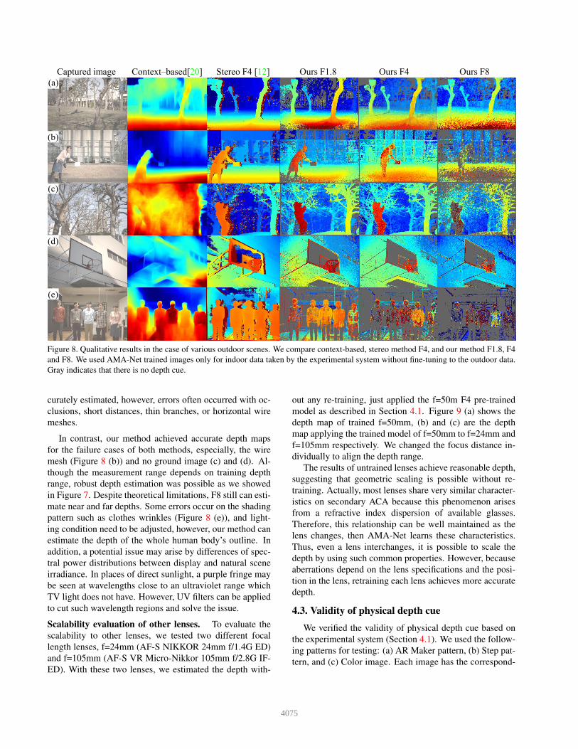
Figure 8. Qualitative results in the case of various outdoor scenes. We compare context-based, stereo method F4, and our method F1.8, F4

and F8. We used AMA-Net trained images only for indoor data taken by the experimental system without fine-tuning to the outdoor data.

Gray indicates that there is no depth cue.

curately estimated, however, errors often occurred with oc-

clusions, short distances, thin branches, or horizontal wire

meshes.

In contrast, our method achieved accurate depth maps

for the failure cases of both methods, especially, the wire

mesh (Figure 8 (b)) and no ground image (c) and (d). Al-

though the measurement range depends on training depth

range, robust depth estimation was possible as we showed

in Figure 7. Despite theoretical limitations, F8 still can esti-

mate near and far depths. Some errors occur on the shading

pattern such as clothes wrinkles (Figure 8 (e)), and light-

ing condition need to be adjusted, however, our method can

estimate the depth of the whole human body’s outline. In

addition, a potential issue may arise by differences of spec-

tral power distributions between display and natural scene

irradiance. In places of direct sunlight, a purple fringe may

be seen at wavelengths close to an ultraviolet range which

TV light does not have. However, UV filters can be applied

to cut such wavelength regions and solve the issue.

Scalability evaluation of other lenses. To evaluate the

scalability to other lenses, we tested two different focal

length lenses, f=24mm (AF-S NIKKOR 24mm f/1.4G ED)

and f=105mm (AF-S VR Micro-Nikkor 105mm f/2.8G IF-

ED). With these two lenses, we estimated the depth with-

out any re-training, just applied the f=50m F4 pre-trained

model as described in Section 4.1. Figure 9 (a) shows the

depth map of trained f=50mm, (b) and (c) are the depth

map applying the trained model of f=50mm to f=24mm and

f=105mm respectively. We changed the focus distance in-

dividually to align the depth range.

The results of untrained lenses achieve reasonable depth,

suggesting that geometric scaling is possible without re-

training. Actually, most lenses share very similar character-

istics on secondary ACA because this phenomenon arises

from a refractive index dispersion of available glasses.

Therefore, this relationship can be well maintained as the

lens changes, then AMA-Net learns these characteristics.

Thus, even a lens interchanges, it is possible to scale the

depth by using such common properties. However, because

aberrations depend on the lens specifications and the posi-

tion in the lens, retraining each lens achieves more accurate

depth.

4.3. Validity of physical depth cue

We verified the validity of physical depth cue based on

the experimental system (Section 4.1). We used the follow-

ing patterns for testing: (a) AR Maker pattern, (b) Step pat-

tern, and (c) Color image. Each image has the correspond-

4075

(c) Untrained f=105mm(a) Trained f=50mm (b) Untrained f=24mm

Figure 9. Scailability evaluation of three different focal length lenses: (a) Trained f=50mm, (b) Untrained f=24mm, and (c) Untrained

f=105mm. All lenses were set to F4.

ing distance; thus, one image ideally has uniform depth.

Figure 10 shows that our method correctly estimated depth

of the near and far plane because the images show a uni-

form color for the corresponding plane, even there is no

contextual information image as Figure 10 (b). Therefore,

our method was not deceived by contextual information; we

verified the validity of using aberrations as a depth cue.

4.4. Validity of AMA-Net’s Positional branch

We tested the pre-trained model with and without a po-

sitional branch in AMA-Net (described in Section 3.3) in

order to verify the validity of positional branch. We fixed

the lens aperture F1.8. Figure 11 (a) presents an example

of sampled A-Map. As can be observed from Figure 11

(a), the shape of PSF varies depending on the position. We

chose the stripe pattern image, to simply analyze the posi-

tion dependence of aberrations. The comparison of with and

without a positional branch on depth estimation are shown

in Figure 11 (b) and (c). The results demonstrated that the

pre-trained model with the positional branch correctly (uni-

formly) estimated the depth, whereas many errors occurred

on without the positional branch depth. The mean error of

with positional branch is 10.0mm, that is about 2.5 times

smaller than the error of without position branch (mean er-

ror: 25.1mm). As the result, we verified that the positional

branch of AMA-Net can efficiently analyze all aberrations

simultaneously.

5. Discussions

We have already presented the performance of our

method above. From here, to discuss the validity of our

method, we carried out simulation study, and then verified

the following two items:

(1) Discrimination ability of various aberrations.

(2) Effectiveness of aberration type.

5.1. Simulation framework

We introduced a simulation framework, as shown in Fig-

ure 12. First, we convolved the PSF kernel obtained by

the system (Figure 5) into the focus image to simulate the

defocused image. We used the measured PSF because of

the difficulty involved in simulating the lens (image) posi-

tional dependence on PSF. Variations of PSF to simulate

Near Captured image Far

(a)

(c)

(b)

Figure 10. Estimated uniform depth of near and far plane.

(b) OFF (c) ON(a) Sampled A-map

Figure 11. Comparison of estimated depth with and without the

positional branch. (a) The sampled A-Map, (b) Without the posi-

tional branch, and (c) With the positional branch of AMA-Net.

defocused image are also shown in Figure 12 (A) - (E).

The magnified images demonstrated the purple and green

fringe on the edge of the near and far image which is equiv-

alent to Figure 2 (E). Secondly, the simulated defocus im-

age is passed to AMA-Net. As defocus images, we used

MSCOCO dataset with a size of 1845x1232 pixels to match

the experimental settings (Figure 5). Next, the simulated

defocused images are input to AMA-Net for testing the pre-

trained model, and finally depth accuracy is estimated.

5.2. Discrimination ability of AMA-Net (sim)

To verify the AMA-Net’s ability to discriminate vari-

ous types of aberrations, first, defocused images were sim-

ulated using three types of PSF: (A) Mathematically de-

fined pillbox shape, (B) Actual PSF at the image center,

and (C) Actual PSF at the corner of the image (Figure 12).

Next, we trained AMA-Net with (A) - (C) individually, then

compared the estimated depth values under the following

five conditions: (a) pre-trained A-model with A image, (b)

pre-trained B-model with B image, (c) pre-trained C-model

4076

z

Simulated defocus image

near

far

Train100 distances

conv

All-focused color image

near far

Accuracy

comparison

in different

conditions

Distance

estimation

AMA-Net

Test AMA-Net

Pre-trained model

……………PSFs for 100 distances

Near

Far

Example of simulated image

(B) RGB-C

(C) RGB-E

(E) Mono-E

(D) Mono-C

(A) Pillbox

PSFs

Figure 12. Simulation framework for depth estimation based on

AMA-Net. We used five PSF variations: (A) pillbox and (B) - (E),

the designations of which are RGB for full color PSF, Mono for

Monochromatic PSF whose shape is the same as that of the Green

PSF, C for Center of the image, and E for corner of the image.

with C image, (d) pre-trained B-model with C image, and

(e) pre-trained C-model with B image. Only A is convo-

luted with a simulated PSF based on Equation 1, and the

shape of which is pill box, imitating an ideal lens. B and C

uses the center and corner PSF of the lens. In the case of (a)

- (c) pre-trained models of PSF use for training and testing

are identical, while (d) and (e) are cross-test to verify that

AMA-Net is distinguishing different PSF shapes. Note that

one type of PSF is convoluted in one entire image to indi-

vidually verify aberration type only for simulation study.

Figure 13 shows the comparison of the estimated depth

vs ground truth in the respective conditions (a) - (e). As for

the results, (a) cannot accurately estimate distance because

the ideal lens has no aberration synonymous with lack of

depth cue. Moreover, (d) and (e) also have large errors in

both the near and far planes, whereas (b) and (c) accurately

estimate distance (equivalent to ideal line). However, (b) -

(e) have slight difference near the in-focus plane because of

the smallness of the PSF. From the results, AMA-Net can

distinguish differences during analysis of the PSF.

5.3. Effectiveness of aberrations (sim)

To verified the effectiveness of aberrations, we compared

the mean error of depth with various PSF shapes. Techni-

cally, aberrations have a position dependence on the lens

(described in Section 3.2); therefore, we used following

PSF kernels in training and testing images: (B) on-axis

RGB-PSF, (C) on-axis Mono-PSF, (D) off-axis RGB-PSF,

and (E) off-axis Mono-PSF, as shown in Figure 12 (B) - (E).

RGB-PSF includes both a CA and MA feature, whereas,

Mono-PSF has only MA. In this verification, we individu-

ally train our AMA-Net with images of (B) - (E) with F1.8

Ground truth[mm]

Est

imat

ed d

epth

[m

m]

1800

1700

1600

1500

1400

13001300 1400 1500 1600 1700 1800

ref

(a) Ideal lens (Pillbox kernel)

(b) C-model x C-PSF

(c) E-model x E-PSF

(d) C-model x E-PSF

(e) E-model x C-PSF

Figure 13. Comparison of estimated depth vs ground truth in five

different conditions.

Dep

th m

ean e

rro

r [m

m]

CA

MA

CA

MA

On-axis PSF Off-axis PSF

CA

MA

MA

CA8.8

16.8 9.825.6

46.154.7

126.8143.0

160

140

120

100

60

40

20

0

80

Figure 14. Comparison of estimated depth mean error on eight

different types of PSF such as CA and MA in both on-axis and

off-axis with F1.8 and F4, respectively.

and F4 PSF (see Figure 3). Figure 14 shows the compari-

son of the above four conditions of each F1.8 and F4 on the

mean error of depth.

From the results, containing only MA still can be utilized

as a depth cue; however, CA achieves even higher accuracy.

Furthermore, on-axis and off-axis results denote the same

tendency of depth mean error. That is to say, AMA-Net can

analyze various types of aberration. Finally, we verified the

effectiveness of CA and MA as a depth cue.

6. Conclusion

We have presented a novel method for passive single-

shot depth measurement using only an off-the-shelf camera

without customization or additional supportive devices. We

have verified that A-Map, which contains various types of

aberrations and distance information, can be utilized as a

depth cue. We also have proposed AMA-Net that is addi-

tionally equipped with a self-attention-to-position mecha-

nism to focus on only the aberration feature of A-Map. We

demonstrated the effectiveness of A-Map for depth mea-

surement through experimental and simulation analyses.

The results of the experiments, supports this approach’s

achievement of highly accurate depth measurement and

highly robust performance.

4077

References

[1] OpenCV. https://opencv.org/. 5

[2] Amir Atapour-Abarghouei and Toby P. Breckon. Real-time

monocular depth estimation using synthetic data with do-

main adaptation via image style transfer. In The IEEE

Conference on Computer Vision and Pattern Recognition

(CVPR), June 2018. 1, 2, 4

[3] Christian Bailer, Tewodros Habtegebrial, Didier Stricker,

et al. Fast feature extraction with cnns with pooling layers.

arXiv preprint arXiv:1805.03096, 2018. 4

[4] Christian Bailer, Kiran Varanasi, and Didier Stricker. Cnn

based patch matching for optical flow with thresholded hinge

loss. arXiv preprint arXiv:1607.08064, 2016. 4

[5] Yosuke Bando, Bing-Yu Chen, and Tomoyuki Nishita. Ex-

tracting depth and matte using a color-filtered aperture. ACM

Transactions on Graphics (TOG), 27(5):134, 2008. 1, 2, 4

[6] Alexander Buslaev, Alex Parinov, Eugene Khvedchenya,

Vladimir I Iglovikov, and Alexandr A Kalinin. Albumenta-

tions: fast and flexible image augmentations. arXiv preprint

arXiv:1809.06839, 2018. 5

[7] Ayan Chakrabarti and Todd Zickler. Depth and deblurring

from a spectrally-varying depth-of-field. In European Con-

ference on Computer Vision, pages 648–661. Springer, 2012.

1, 2, 4

[8] Jia-Ren Chang and Yong-Sheng Chen. Pyramid stereo

matching network. In Proceedings of the IEEE Conference

on Computer Vision and Pattern Recognition, pages 5410–

5418, 2018. 4

[9] Josep Garcia, Juan M. Sanchez, Xavier Orriols, and Xavier

Binefa. Chromatic aberration and depth extraction. In Pro-

ceedings 15th International Conference on Pattern Recogni-

tion. ICPR-2000, volume 1, pages 762–765, 2000. 1

[10] Kaiming He, Xiangyu Zhang, Shaoqing Ren, and Jian Sun.

Deep residual learning for image recognition. In Proceed-

ings of the IEEE conference on computer vision and pattern

recognition, pages 770–778, 2016. 4

[11] Alex Hernandez-Garcıa and Peter Konig. Do deep nets

really need weight decay and dropout? arXiv preprint

arXiv:1802.07042, 2018. 4

[12] Heiko Hirschmuller. Accurate and efficient stereo processing

by semi-global matching and mutual information. In Com-

puter Vision and Pattern Recognition, 2005. CVPR 2005.

IEEE Computer Society Conference on, volume 2, pages

807–814. IEEE, 2005. 5

[13] Alex Kendall, Hayk Martirosyan, Saumitro Dasgupta, Peter

Henry, Ryan Kennedy, Abraham Bachrach, and Adam Bry.

End-to-end learning of geometry and context for deep stereo

regression. CoRR, vol. abs/1703.04309, 2017. 4

[14] Sangjin Kim, Eunsung Lee, Monson H Hayes, and Joonki

Paik. Multifocusing and depth estimation using a color shift

model-based computational camera. IEEE Transactions on

Image Processing, 21(9):4152–4166, 2012. 1, 2

[15] Diederik P Kingma and Jimmy Ba. Adam: A method for

stochastic optimization. arXiv preprint arXiv:1412.6980,

2014. 4

[16] Alex Krizhevsky, Ilya Sutskever, and Geoffrey E Hinton.

Imagenet classification with deep convolutional neural net-

works. In Advances in neural information processing sys-

tems, pages 1097–1105, 2012. 5

[17] Yevhen Kuznietsov, Jorg Stuckler, and Bastian Leibe. Semi-

supervised deep learning for monocular depth map predic-

tion. In Proc. of the IEEE Conference on Computer Vision

and Pattern Recognition, pages 6647–6655, 2017. 1, 2, 4

[18] Yann A LeCun, Leon Bottou, Genevieve B Orr, and Klaus-

Robert Muller. Efficient backprop. In Neural networks:

Tricks of the trade, pages 9–48. Springer, 2012. 4

[19] Seungwon Lee, Nahyun Kim, Kyungwon Jung, Monson H

Hayes, and Joonki Paik. Single image-based depth estima-

tion using dual off-axis color filtered aperture camera. In

Acoustics, Speech and Signal Processing (ICASSP), 2013

IEEE International Conference on, pages 2247–2251. IEEE,

2013. 1, 2

[20] Zhengqi Li and Noah Snavely. Megadepth: Learning single-

view depth prediction from internet photos. In Proceedings

of the IEEE Conference on Computer Vision and Pattern

Recognition, pages 2041–2050, 2018. 5

[21] Wenjie Luo, Alexander G Schwing, and Raquel Urtasun. Ef-

ficient deep learning for stereo matching. In Proceedings

of the IEEE Conference on Computer Vision and Pattern

Recognition, pages 5695–5703, 2016. 4

[22] Carvalho Marcela, Saux Bertrand Le, Trouve-Peloux

Pauline, Almansa Andres, and Champagnat Frederic. Deep

depth from defocus: How can defocus blur improve 3d esti-

mation using dense neural networks?? european conference

on computer vision, pages 307–323, 2018. 1, 2

[23] Manuel Martinello, Andrew Wajs, Shuxue Quan, Hank Lee,

Chien Lim, Taekun Woo, Wonho Lee, Sang-Sik Kim, and

David Lee. Dual aperture photography: image and depth

from a mobile camera. In Computational Photography

(ICCP), 2015 IEEE International Conference on, pages 1–

10. IEEE, 2015. 1, 2, 4

[24] Yusuke Moriuchi, Takayuki Sasaki, Nao Mishima, and

Takeshi Mita. 23-4: Invited paper: Depth from asymmet-

ric defocus using color-filtered aperture. In SID Symposium

Digest of Technical Papers, volume 48, pages 325–328. Wi-

ley Online Library, 2017. 1, 2, 4

[25] Vladimir Paramonov, Ivan Panchenko, Victor Bucha, An-

drey Drogolyub, and Sergey Zagoruyko. Depth camera

based on color-coded aperture. In Proceedings of the IEEE

Conference on Computer Vision and Pattern Recognition

Workshops, pages 1–9, 2016. 1, 2, 4

[26] Edgar Simo-Serra, Eduard Trulls, Luis Ferraz, Iasonas

Kokkinos, Pascal Fua, and Francesc Moreno-Noguer. Dis-

criminative learning of deep convolutional feature point de-

scriptors. In Proceedings of the IEEE International Confer-

ence on Computer Vision, pages 118–126, 2015. 4

[27] Murali Subbarao and Gopal Surya. Depth from defocus: a

spatial domain approach. International Journal of Computer

Vision, 13(3):271–294, 1994. 2

[28] Pauline Trouve, Frederic Champagnat, Guy Le Besnerais,

Jacques Sabater, Thierry Avignon, and Jereme Idier. Pas-

sive depth estimation using chromatic aberration and a depth

4078

from defocus approach. Applied optics, 52(29):7152–7164,

2013. 1, 2

[29] Oriol Vinyals, Alexander Toshev, Samy Bengio, and Du-

mitru Erhan. Show and tell: Lessons learned from the 2015

mscoco image captioning challenge. IEEE transactions on

pattern analysis and machine intelligence, 39(4):652–663,

2017. 5

[30] Sergey Zagoruyko and Nikos Komodakis. Learning to com-

pare image patches via convolutional neural networks. In

Proceedings of the IEEE Conference on Computer Vision

and Pattern Recognition, pages 4353–4361, 2015. 4

[31] Jure Zbontar and Yann LeCun. Stereo matching by training

a convolutional neural network to compare image patches.

Journal of Machine Learning Research, 17(1-32):2, 2016. 4

[32] Han Zhang, Ian Goodfellow, Dimitris Metaxas, and Augus-

tus Odena. Self-attention generative adversarial networks.

arXiv preprint arXiv:1805.08318, 2018. 4

[33] Zhun Zhong, Liang Zheng, Guoliang Kang, Shaozi Li, and

Yi Yang. Random erasing data augmentation. arXiv preprint

arXiv:1708.04896, 2017. 5

4079