UNIVERSITY OF SYDNEY SCHOOL OF GEOSCIENCES

DIVISION OF GEOLOGY AND GEOPHYSICS

Deep Ear th Structure and Global Tectonics

GEOL 2001 Geological Hazards and Solutions

Semester 1

2002

R. Dietmar Müller

I

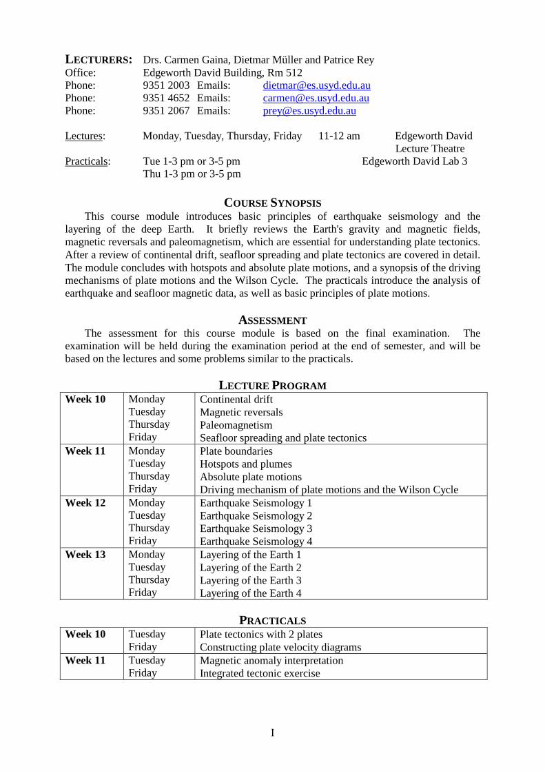
LECTURERS: Drs. Carmen Gaina, Dietmar Müller and Patrice Rey Off ice: Edgeworth David Building, Rm 512 Phone: 9351 2003 Emails: dietmar@es.usyd.edu.au Phone: 9351 4652 Emails: carmen@es.usyd.edu.au Phone: 9351 2067 Emails: prey@es.usyd.edu.au Lectures: Monday, Tuesday, Thursday, Friday 11-12 am Edgeworth David Lecture Theatre Practicals: Tue 1-3 pm or 3-5 pm Edgeworth David Lab 3 Thu 1-3 pm or 3-5 pm

COURSE SYNOPSIS

This course module introduces basic principles of earthquake seismology and the layering of the deep Earth. It briefly reviews the Earth's gravity and magnetic fields, magnetic reversals and paleomagnetism, which are essential for understanding plate tectonics. After a review of continental drift, seafloor spreading and plate tectonics are covered in detail . The module concludes with hotspots and absolute plate motions, and a synopsis of the driving mechanisms of plate motions and the Wilson Cycle. The practicals introduce the analysis of earthquake and seafloor magnetic data, as well as basic principles of plate motions.

ASSESSMENT

The assessment for this course module is based on the final examination. The examination will be held during the examination period at the end of semester, and will be based on the lectures and some problems similar to the practicals.

LECTURE PROGRAM

Week 10 Monday Tuesday Thursday Friday

Continental drift Magnetic reversals Paleomagnetism Seafloor spreading and plate tectonics

Week 11 Monday Tuesday Thursday Friday

Plate boundaries Hotspots and plumes Absolute plate motions Driving mechanism of plate motions and the Wilson Cycle

Week 12 Monday Tuesday Thursday Friday

Earthquake Seismology 1 Earthquake Seismology 2 Earthquake Seismology 3 Earthquake Seismology 4

Week 13 Monday Tuesday Thursday Friday

Layering of the Earth 1 Layering of the Earth 2 Layering of the Earth 3 Layering of the Earth 4

PRACTICALS

Week 10 Tuesday Friday

Plate tectonics with 2 plates Constructing plate velocity diagrams

Week 11 Tuesday Friday

Magnetic anomaly interpretation Integrated tectonic exercise

II

BIBLIOGRAPHY KEAREY, P., AND VINE, F.J., 1996, GLOBAL TECTONICS, BLACKWELL

SCIENCE INC., 344 P.

Table of contents

CONTINENTAL DRIFT 1

INTRODUCTION 1 WEGENER’S THEORY 2 EVIDENCE FOR CONTINENTAL DRIFT: 3 DEVELOPING THE THEORY 3

THE EARTH' S MAGNETIC FIELD 4

INTRODUCTION 4 ORIGIN OF THE EARTH’S MAGNETIC FIELD 4 ENERGY SOURCES FOR DRIVING CONVECTION IN THE OUTER CORE. 5 CHARACTER OF THE MAGNETIC FIELD 5 GEOMAGNETIC FIELD REVERSALS 10 PALEOMAGNETISM 11 MAGNETOSTRATIGRAPHY 11 PAST AND PRESENT GEOMAGNETIC FIELD 12

THE DEVELOPMENT OF THE PLATE TECTONIC THEORY 15

OCEAN FLOOR MAPPING 15 INTRODUCTION 15 MAGNETIC STRIPING AND POLAR REVERSALS 17 MAPPING THE OCEANIC MAGNETIC FIELD 18

MARINE MAGNETIC ANOMALIES: HOW DO THEY WORK? 20 INTRODUCTION 20 SHAPE AND INTENSITY OF SEAFLOOR MAGNETIC ANOMALIES 21 DEEP SEA DRILLING 24 CONCENTRATION OF EARTHQUAKES 24 MARINE GRAVITY ANOMALIES FROM SATELLITE ALTIMETRY 25

THE THEORY OF PLATE TECTONICS 26 INTRODUCTION 26 PLATE TECTONIC CONCEPTS: 27

(1) Continuity of plate boundaries 27 (2) Rigidity 27 (3) Relative motion 27

MATHEMATICAL FOUNDATION OF PLATE TECTONICS 29 FORMAL HYPOTHESIS OF PLATE TECTONICS 30

PLATE BOUNDARIES 30 DIVERGENT BOUNDARIES 30 CONVERGENT BOUNDARIES 32

Oceanic-continental convergence 33 Oceanic-oceanic convergence 35 Continental-continental convergence 37 Back arc basins 38 Arc-continent collision 38

III

Suspect terrains 39 TRANSFORM BOUNDARIES 39 FRACTURE ZONES 41 FRACTURE ZONE MODEL 43 TRIPLE JUNCTIONS 43

Introduction 43 Summary 45

PLATE-BOUNDARY ZONES 46 RATES OF MOTION 47 PLATE MOTIONS SINCE THE LATE JURASSIC 48

HOTSPOTS 51 HAWAII 51 PLUME THEORY 52 LARGE IGNEOUS PROVINCES (LIPS) 53 SEAMOUNT CHAINS 57

ABSOLUTE PLATE MOTIONS 58 METHODS FOR RECONSTRUCTING "ABSOLUTE" PLATE MOTIONS 58 THE FIXED HOTSPOT HYPOTHESIS 59 APPARENT POLAR WANDERING 60

DRIVING MECHANISM OF PLATE MOTIONS 61 MANTLE DRAG FORCE 61 CONTINENTAL DRAG FORCE 61 RIDGE PUSH FORCE 62 SLAB PULL FORCE 62 SLAB RESISTING FORCE 63 TRENCH SUCTION FORCE 63 COLLISIONAL RESISTANCE FORCE 63 TRANSFORM FAULT RESISTANCE FORCE 64 TECTONIC STRESSES AND THEIR RELATIONSHIP TO PLATE DRIVING FORCES 65

THE WILSON CYCLE 70 1) FORMATION OF RIFT 70 2) EXTENSION AND FORMATION OF RIFT VALLEYS 70 3) YOUNG OCEAN BASIN 71 4) MATURE OCEAN BASIN 72 5) CLOSING OF THE OCEAN 72 6) COLLISION 74 7) RENEWED BREAKUP 75

DEEP EARTH STRUCTURE AND SEISMOLOGY 76

FOCAL MECHANISM SOLUTIONS 76 WHY? 76 HOW IS IT DONE? 76 ELASTIC REBOUND THEORY 76 DISLOCATION MODEL FOR AN EARTHQUAKE 77

INTRODUCTION 85

EARTHQUAKE SEISMOLOGY 85

INTRODUCTION 85 MEASURING EARTHQUAKES 86 BODY WAVES 86

IV

SURFACE WAVES 87 EARTHQUAKE DESCRIPTORS 88

FOCAL DEPTH 88 EPICENTER 88 MAGNITUDE 88

Richter scale 88 Surface wave magnitude 89 Body wave magnitude 90 Why so many magnitude scales? 90 What is earthquake moment? 90

FOCAL MECHANISM SOLUTIONS 93 WHY? 93 HOW IS IT DONE? 93 ELASTIC REBOUND THEORY 93 DISLOCATION MODEL FOR AN EARTHQUAKE 94

SEISMIC TOMOGRAPHY 102

LAYERING OF THE EARTH: RESULT S FROM SEISMOLOGY AND GEOLOGY 104

CONTINENTAL CRUST 104 COMPOSITION 104 STRUCTURE OF CONTINENTAL CRUST 104

OCEANIC CRUST 106 COMPOSITION 106 STRUCTURE OF THE OCEANIC CRUST 106 OPHIOLITES 106 MAIN DIFFERENCES BETWEEN CONTINENTAL AND OCEANIC CRUST 107

MANTLE 107 OVERVIEW 107 SEISMIC DISCONTINUITIES 107 UPPER MANTLE: DEPTH OF 10-400 KM. 107 TRANSITION REGION: DEPTH OF 400-650 KM. 107 LOWER MANTLE: DEPTH OF 650-2,890 KM. 108

CORE 108 OUTER CORE: DEPTH OF 2,890-5,150 KM. 108 D": DEPTH OF 2,700-2,890. 108 INNER CORE: DEPTH OF 5,150-6,370 KM. 109

DATA ON THE EARTH'S INTERIOR 109

REFERENCES 110

1

GLOBAL TECTONICS CONTINENTAL DRIFT

Introduction In geologic terms, a plate is a large, rigid slab of solid rock. The word tectonics comes from the Greek root "to build." Putting these two words together, we get the term plate tectonics, which refers to how the Earth's surface is built of plates. The theory of plate tectonics states that the Earth's outermost layer is fragmented into a dozen or more large and small plates that are moving relative to one another as they ride atop hotter, more mobile material. The diagrams below show the break-up of the supercontinent Pangaea (meaning "all l ands" in Greek), which figured prominently in the theory of continental drift -- the forerunner to the theory of plate tectonics.

Breakup of Pangaea

Plate tectonics is a relatively new scientific concept, introduced some 30 years ago, but it has revolutionized our understanding of the dynamic planet upon which we live. The theory has unified the study of the Earth by drawing together many branches of the earth sciences, from paleontology (the study of fossils) to seismology (the study of earthquakes). It has provided explanations to questions that scientists had speculated upon for centuries -- such as why earthquakes and volcanic eruptions occur in very specific areas around the world, and how and why great mountain ranges like the Alps and Himalayas formed. The belief that continents have not always been fixed in their present positions was suspected long before the 20th century; this notion was first suggested as early as 1596 by the Dutch map maker Abraham Ortelius in his work Thesaurus Geographicus. Ortelius suggested that the Americas were "torn away from Europe and Africa . . . by earthquakes and floods" and went on to say: "The vestiges of the rupture reveal themselves, if someone brings forward a map of the world and considers carefully the coasts of the three [continents]." Ortelius' idea surfaced again in the 19th century. However, it was not until 1912 that the idea of moving continents was seriously considered as a full -blown scientific theory -- called Continental Drift -- introduced in two articles published by a 32-year-old German meteorologist named Alfred Lothar Wegener.

2

He contended that, around 200 milli on years ago, the supercontinent Pangaea began to split apart. Alexander Du Toit, Professor of Geology at Johannesburg University and one of Wegener's staunchest supporters, proposed that Pangaea first broke into two large continental landmasses, Laurasia in the northern hemisphere and Gondwanaland in the southern hemisphere. Laurasia and Gondwanaland then continued to break apart into the various smaller continents that exist today.

Wegener’s theory Wegener's theory was based in part on what appeared to him to be the remarkable fit of the South American and African continents, first noted by Abraham Ortelius three centuries earlier. Wegener was also intrigued by the occurrences of unusual geologic structures and of plant and animal fossils found on the matching coastlines of South America and Africa, which are now widely separated by the Atlantic Ocean. He reasoned that it was physically impossible for most of these organisms to have swum or have been transported across the vast oceans. To him, the presence of identical fossil species along the coastal parts of Africa and South America was the most compelli ng evidence that the two continents were once joined.

In Wegener's mind, the drifting of continents after the break-up of Pangaea explained not only the matching fossil occurrences but also the evidence of dramatic climate changes on some continents. For example, the discovery of fossils of tropical plants (in the form of coal deposits) in Antarctica led to the conclusion that this frozen land previously must have been situated closer to the equator, in a more temperate climate where lush, swampy vegetation could grow. Other mismatches of geology and climate included distinctive fossil ferns (Glossopteris) discovered in now-polar regions, and the occurrence of glacial deposits in present-day arid Africa, such as the Vaal River valley of South Africa.

The theory of continental drift would become the spark that ignited a new way of viewing the Earth. But at the time Wegener introduced his theory, the scientific community firmly believed the continents and oceans to be permanent features on the Earth's surface. Not surprisingly, his proposal was not well received, even though it seemed to agree with the scientific information available at the time. A fatal weakness in Wegener's theory was that it could not satisfactorily answer the most fundamental question raised by his criti cs: What kind of forces could be strong enough to move such large masses of solid rock over such great distances? Wegener suggested that the continents simply plowed through the ocean floor, but Harold Jeffreys, a noted English geophysicist, argued correctly that it was physically impossible for a large mass of solid rock to plow through the ocean floor without breaking up. Undaunted by rejection, Wegener devoted the rest of his li fe to doggedly pursuing additional evidence to defend his theory. He froze to death in 1930 during an expedition crossing the Greenland ice cap, but the controversy he spawned raged on. However, after his death, new evidence from ocean floor exploration and other studies rekindled interest in Wegener's theory, ultimately leading to the development of the theory of plate tectonics.

3

Evidence for continental dr ift: • Geological evidence: 1) fold belts 2) age provinces 3) igneous provinces 4) stratigraphic sections 5) metallogenic provinces • Paleoclimatic evidence: 1) carbonates and reef deposits 2) evaporites 3) red beds 4) coal and oil 5) phosphorites 6) bauxite and laterite 7) desert deposits 8) glacial deposits • Paleontological evidence 1) distribution of tetrapods 2) early Permian reptile Mesosaurus 3) marine invertebrates 4) Cambrian trilobites 5) ammonites 6) Glossopteris and Gangamopteris fauna 7) diversity of species Plate tectonics has proven to be as important to the Earth sciences as the discovery of the structure of the atom was to physics and chemistry and the theory of evolution was to the li fe sciences. Even though the theory of plate tectonics is now widely accepted by the scientific community, aspects of the theory are still being debated today. Ironically, one of the chief outstanding questions is the one Wegener failed to resolve: What is the nature of the forces propelli ng the plates? Scientists also debate how plate tectonics may have operated (if at all ) earlier in the Earth's history and whether similar processes operate, or have ever operated, on other planets in our solar system.

Developing the theory Continental drift was hotly debated off and on for decades following Wegener's death before it was largely dismissed as being eccentric, preposterous, and improbable. However, beginning in the 1950s, a wealth of new evidence emerged to revive the debate about Wegener's provocative ideas and their implications. In particular, four major scientific developments spurred the formulation of the plate-tectonics theory: (1) demonstration of the ruggedness and youth of the ocean floor; (2) confirmation of repeated reversals of the Earth magnetic field in the geologic past;

4

(3) emergence of the seafloor-spreading hypothesis and associated recycling of oceanic crust; and

(4) precise documentation that the world's earthquake and volcanic activity is concentrated along oceanic trenches and submarine mountain ranges.

THE EARTH'S MAGNETIC FIELD

Introduction The Earth's magnetic field provides us with an essential tool to understand plate tectonics.

The development of the plate tectonic theory is based on two particular properties of the Earth’s magnetic field::

1) The field has changed its or ientation through time. 2) Some rockforming minerals can record properties of the Earth's past magnetic field.

These properties allows tectonic plates to be tracked through time, and played a major role in formulating the model of sea floor-spreading. The field originates in the Earth's outer core and reverses its orientation at irregular time intervals due to convection of electrically conducting material:

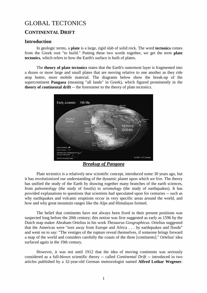
Origin of the Ear th’s magnetic field • The origin of the Earth's magnetic field is due to convection of a electrically conducting

fluid outer core. This is an example of a"homogeneous dynamo", or a dynamo without wires, consisting of currents in a continuum:

• Most likely pattern of convection consists of cylindrical rolls aligned with the Earth's axis

of rotation. Multiple cylindrical rolls are very similar to the currents in a double disk dynamo. Double disk dynamos exhibit irregular magnetic polarity reversals.

5

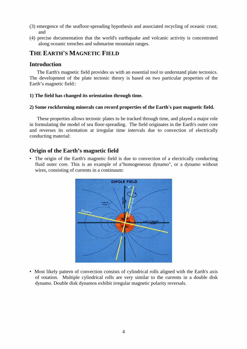
A snapshot of the lines of force of the magnetic field generated in the simulated fluid core of the Earth. (from Glatzmaier & Roberts, 96)

Energy sources for dr iving convection in the outer core. • Radioactivity from, which is the most likelyradiogenic element from solar abundances to

reside in the Earth'score, but not likely to be in a liquid iron solution at core pressure. • Compositional convection, in which heavier iron crystalli zes out ofsolution onto the inner

core boundary, i.e., the inner core isgrowing. Lighter residual element bouyantly rises. Latent heat isreleased as the inner core material crystalli zes. A key test of thishypothesis depends on results from high pressure mineral physics,predicting the density of iron at inner core pressures andtempeartures, and from seismology, measuring with high accuracy theamplitude of compressional waves reflected from the inner core to determinethe density contrast at that boundary.

Character of the magnetic field The Earth's Magnetic Field is pr imar ily a dipole field, exhibiting some small non-dipole components. It has both space and time variations consistent with an origin due to convection in a conducting, fluid outer core.

6

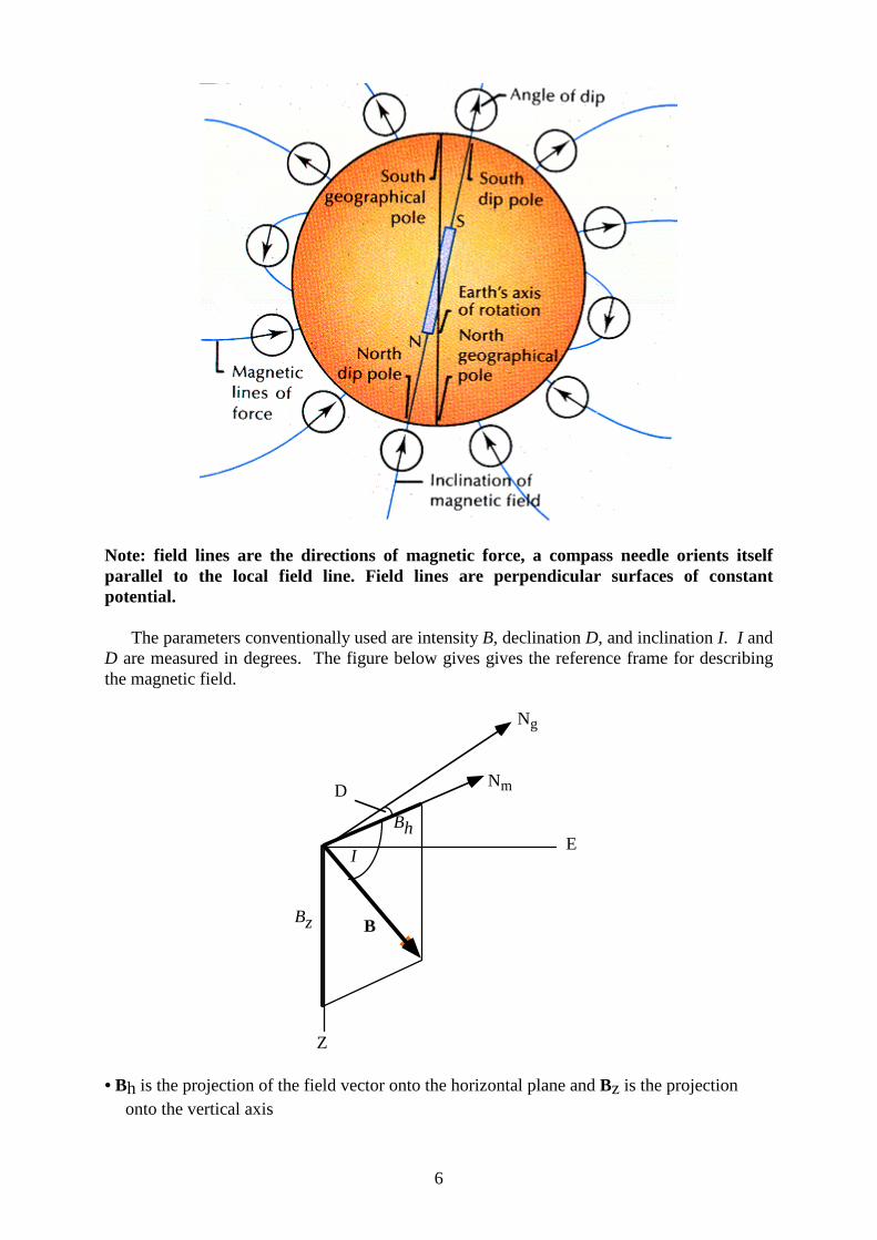
Note: field lines are the directions of magnetic force, a compass needle or ients itself parallel to the local field line. Field lines are perpendicular sur faces of constant potential.

The parameters conventionally used are intensity B, declination D, and inclination I. I and D are measured in degrees. The figure below gives gives the reference frame for describing the magnetic field.

Ng

E

Z

D

Bz

Bh

I

B

Nm

• Bh is the projection of the field vector onto the horizontal plane and Bz is the projection onto the vertical axis

7

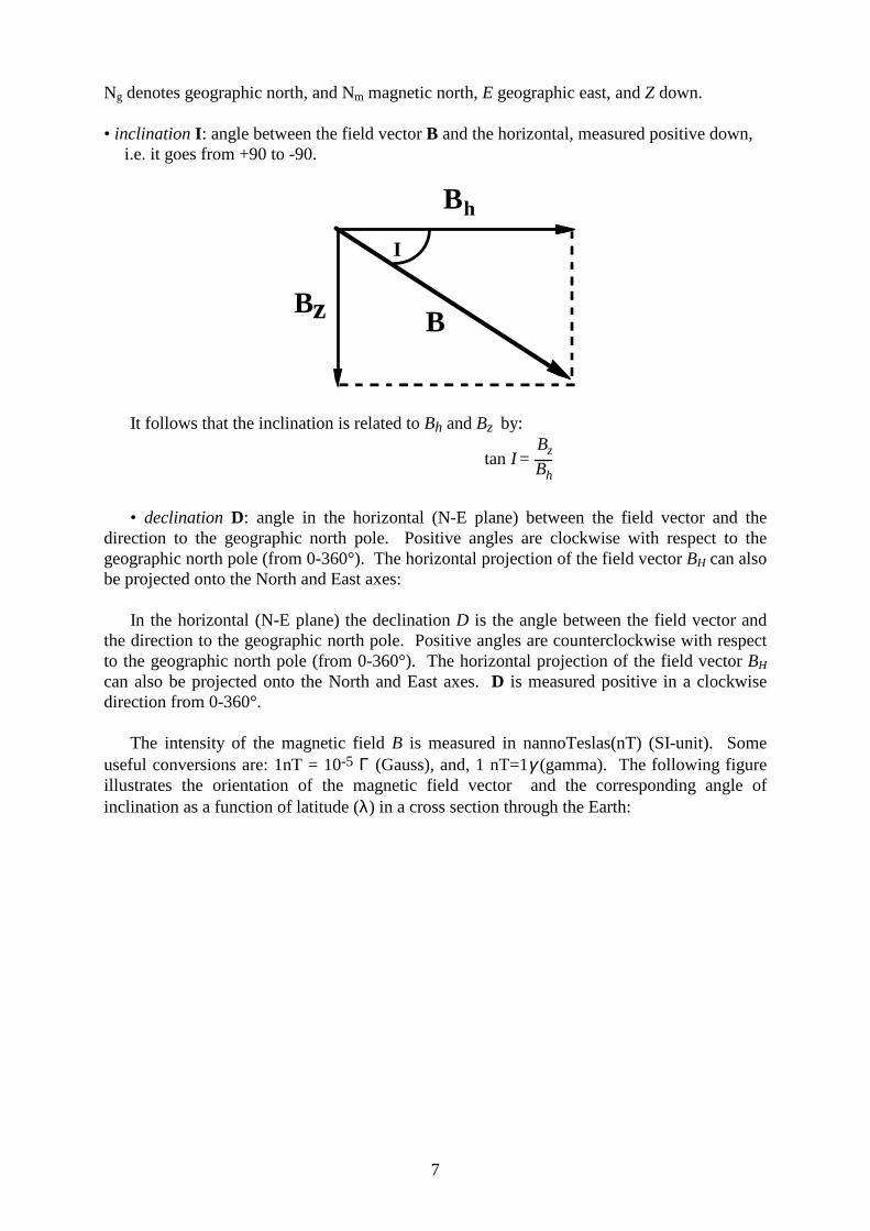
Ng denotes geographic north, and Nm magnetic north, E geographic east, and Z down. • inclination I: angle between the field vector B and the horizontal, measured positive down,

i.e. it goes from +90 to -90.

Bh

Bz B

I

It follows that the inclination is related to Bh and Bz by:

tan I =

Bz

Bh

• declination D: angle in the horizontal (N-E plane) between the field vector and the direction to the geographic north pole. Positive angles are clockwise with respect to the geographic north pole (from 0-360°). The horizontal projection of the field vector BH can also be projected onto the North and East axes:

In the horizontal (N-E plane) the declination D is the angle between the field vector and the direction to the geographic north pole. Positive angles are counterclockwise with respect to the geographic north pole (from 0-360°). The horizontal projection of the field vector BH can also be projected onto the North and East axes. D is measured positive in a clockwise direction from 0-360°.

The intensity of the magnetic field B is measured in nannoTeslas(nT) (SI-unit). Some

useful conversions are: 1nT = 10-5 Γ (Gauss), and, 1 nT=1γ (gamma). The following figure illustrates the orientation of the magnetic field vector and the corresponding angle of inclination as a function of latitude (λ) in a cross section through the Earth:

8

9

North magnetic pole

South magnetic pole

Magneticequator

Magneticdipole

λ

I

–

+

θ

Inclination Colatitude and inclination are related by the dipole formula:

tan I = 2 cot(θ)

θ = 90–λ.

It follows that tan I = 2 tanλ

10

tan (λ ) = (tan I)/2.

Hence there is a straightforward relationship between the inclination of the magnetic field and the magnetic latitude, from which the distance from the magnetic pole can be computed. This is essential for reconstructing tectonic plates.

BH = B cosI

BN = B cosI cosD

BE = BcosI sinD.

• The geomagnetic poles are presently at 79°N, 71°W and 79°S, 109°E.

Geomagnetic field reversals • the Earth's dipole field flips polarity at irregular intervals • the polarity is said to be "normal" when it is oriented the same as today • on average, the field spends about half its time in each state • reversals are observed from Precambrian times to the present although the frequency of

reversals has changed considerably through time

• during a reversal, the intensity usually decreases by about an order of magnitude for several

thousand years, while the field maintains its direction. • the field then undergoes complicated directional changes over a period of 1000-4000 years

and finally intensity grows with the field having reversed polarity • the total time span of a reversal is up to 10.000 years • the reversal sequence has been calibrated for the last 5 milli on years by dating basalts of

known polarity. • portions of the time scale which are of one dominant polarity are called chrons, and the most

recent four chrons are named after scientists who contributed significantly to our understanding of the geomagnetic field (Brunhes, Matuyama, Gauss, Gilbert).

11

• Portions of the time scale which are of one dominant polarity are called chrons.

Paleomagnetism

Study of fossil magnetism retained in rocks

• paramagnetic minerals retain a record of the past direction of the earth's magnetic field • induced magnetization is lost when substance is removed from field • ferromagnetic magnetization below the Curie temperature (~580°C for magnetite, ~680° for

Hematite) -> permanent or remanent magnetism • TRM (thermoremanent magnetization) • DRM (detrital remanent magnetization) • CRM (chemical remanent magnetization) • VRM (viscous remanent magnetization)

Magnetostratigraphy • Cox et al. (1968) measured the remanent magnetization of lavas from land sites • Basalts were dated by a radiometric technique called potassium-argon method, which

allowed a reconstruction of a reversal time scale back to 4.5 Ma ("Ma" stands for the Latin "Megannum", and is used in the literature as meaning "milli on years before present"). For earlier ages the errors in the dating method were too large.

• By combining the dating of rocks with different polarity onshore (and offshore) with the

mapping of lineated magnetic anomaly sequences on ocean crust, a reversal timescale can be constructed.

12

• paleomagnetic investigation of deep sea cores (using detrital remanent magnetism of

sediments) was used to extend the timescale back to 20 Ma by Opdyke et al (1974).

• meanwhile even the oldest preserved ocean crust (~180Ma, west Pacific) has been

surveyed and drill ed, extending the magnetic timescale to about the Middle Jurassic. • paleomagnetic investigations on land have shown that geomagnetic reversals have

occurred at least back to 2.1 Ga ("Gigannum", billi on years before present).

The first magnetic polarity timescale for the Late Cretaceous to Quaternary was constructed by Heirtzler et al. (1968). They used magnetic anomalies along a single ship track in the South Atlantic to calibrate their timescale by assuming that seafloor spreading rates had been approximately constant.

This timescale underwent only minor changes until Cande and Kent (1992) undertook a

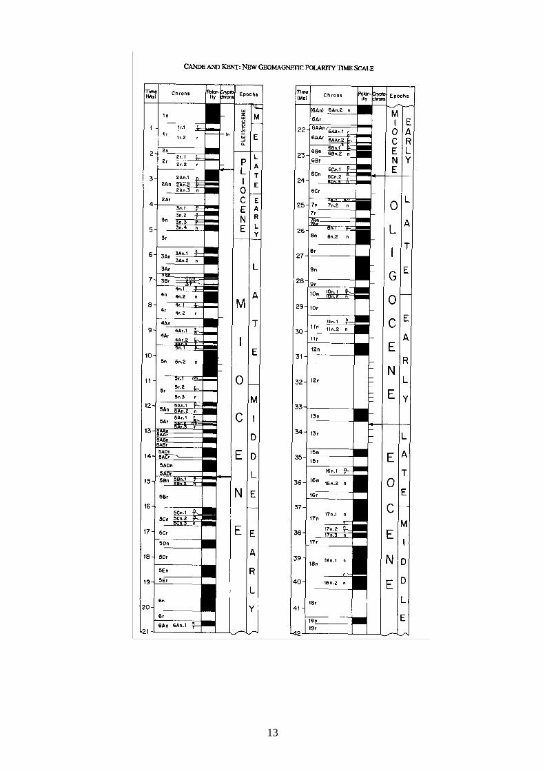
systematic analysis of magnetic anomalies in different ocean basins. Instead of assuming constant spreading rates between any particular plates, they produced a composite record from radiometrically and biostratigraphically determined age tiepoints and smoothly varying seafloor spreading rates in different oceans. Recently, this timescale underwent minor changes by incorporating more age tiepoints (Cande and Kent , 1995).

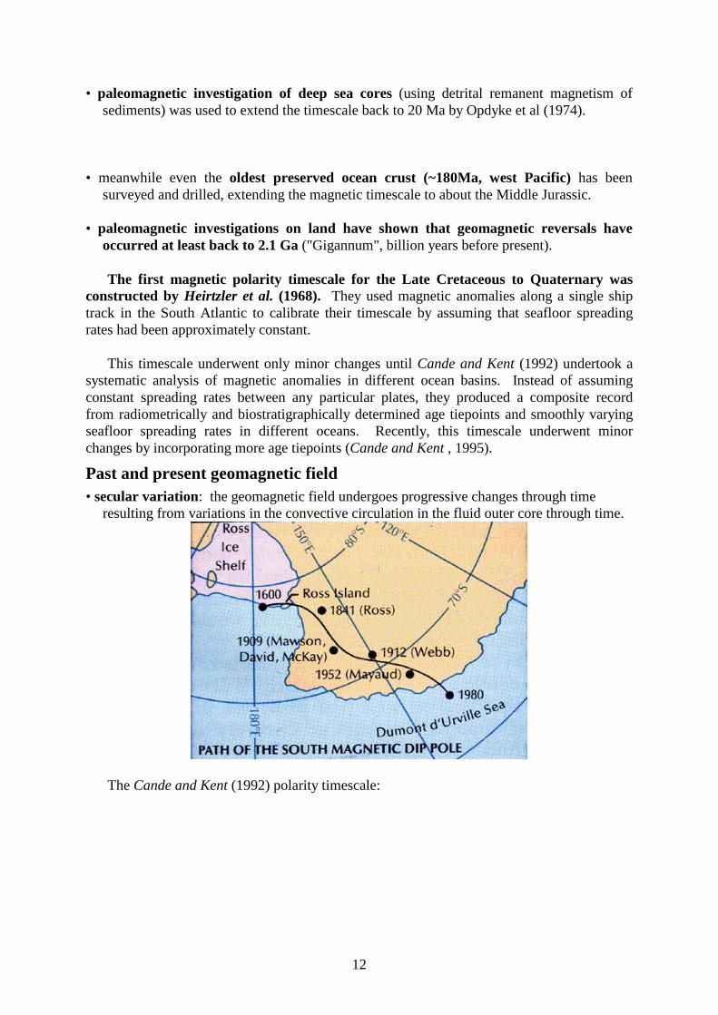
Past and present geomagnetic field • secular variation: the geomagnetic field undergoes progressive changes through time

resulting from variations in the convective circulation in the fluid outer core through time.

The Cande and Kent (1992) polarity timescale:

13

14

15

• paleomagnetic measurements provide intensity, declination, and inclination of the primary

remanent magnetization, given the assumption that the Earth's magnetic field averages a dipole field in geological time spans

• inclination is related to paleolatitude • declination is related to rotation • paleolongitudes of a continent can never be resolved due to radial symmetry of

magnetic field Apparent polar wandering (APW) curves can be used to interpret motions, colli sons, and disruptions of continents.

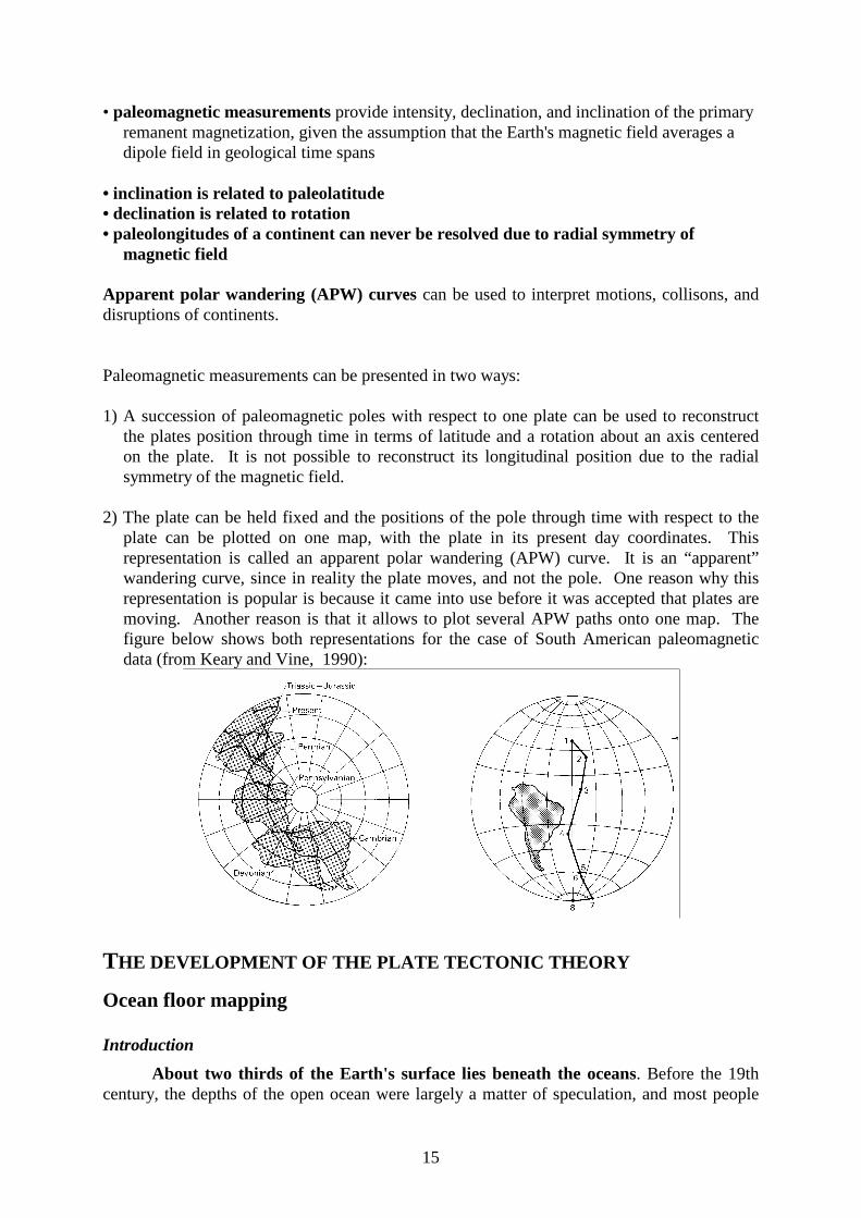
Paleomagnetic measurements can be presented in two ways: 1) A succession of paleomagnetic poles with respect to one plate can be used to reconstruct

the plates position through time in terms of latitude and a rotation about an axis centered on the plate. It is not possible to reconstruct its longitudinal position due to the radial symmetry of the magnetic field.

2) The plate can be held fixed and the positions of the pole through time with respect to the

plate can be plotted on one map, with the plate in its present day coordinates. This representation is called an apparent polar wandering (APW) curve. It is an “apparent” wandering curve, since in reality the plate moves, and not the pole. One reason why this representation is popular is because it came into use before it was accepted that plates are moving. Another reason is that it allows to plot several APW paths onto one map. The figure below shows both representations for the case of South American paleomagnetic data (from Keary and Vine, 1990):

THE DEVELOPMENT OF THE PLATE TECTONIC THEORY

Ocean floor mapping

Introduction

About two thirds of the Earth's sur face lies beneath the oceans. Before the 19th century, the depths of the open ocean were largely a matter of speculation, and most people

16

thought that the ocean floor was relatively flat and featureless. However, as early as the 16th century, a few intrepid navigators, by taking soundings with hand lines, found that the open ocean can differ considerably in depth, showing that the ocean floor was not as flat as generally believed. Oceanic exploration during the next centuries dramatically improved our knowledge of the ocean floor. We now know that most of the geologic processes occurring on land are linked, directly or indirectly, to the dynamics of the ocean floor. "Modern" measurements of ocean depths greatly increased in the 19th century, when deep-sea line soundings (bathymetric surveys) were routinely made in the Atlantic and Caribbean. In 1855, a bathymetric chart published by U.S. Navy Lieutenant Matthew Maury revealed the first evidence of underwater mountains in the central Atlantic (which he called "Middle Ground"). This was later confirmed by survey ships laying the trans-Atlantic telegraph cable. Our picture of the ocean floor greatly sharpened after World War I (1914-18), when echo-sounding devices -- primitive sonar systems -- began to measure ocean depth by recording the time it took for a sound signal (commonly an electrically generated "ping") from the ship to bounce off the ocean floor and return. Time graphs of the returned signals revealed that the ocean floor was much more rugged than previously thought. Such echo-sounding measurements clearly demonstrated the continuity and roughness of the submarine mountain chain in the central Atlantic (later called the Mid-Atlantic Ridge) suggested by the earlier bathymetric measurements.

Global mid-ocean ridge system

In 1947, seismologists on the U.S. research ship Atlantis found that the sediment layer on the floor of the Atlantic was much thinner than originally thought. Scientists had previously believed that the oceans have existed for at least 4 billion years, so therefore the sediment layer should have been very thick. Why then was there so little accumulation of sedimentary rock and debris on the ocean floor? The answer to this question, which came after further exploration, would prove to be vital to advancing the concept of plate tectonics. In the 1950s, oceanic exploration greatly expanded. Data gathered by oceanographic surveys conducted by many nations led to the discovery that a great mountain range on the

17

ocean floor virtually encircled the Earth. Called the global mid-ocean ridge, this immense submarine mountain chain -- more than 50,000 kilometers (km) long and, in places, more than 800 km across -- zig-zags between the continents, winding its way around the globe like the seam on a baseball. Rising an average of about 4,500 meters(m) above the sea floor, the mid-ocean ridge overshadows all the mountains in the United States except for Mount McKinley (Denali) in Alaska (6,194 m). Though hidden beneath the ocean surface, the global mid-ocean ridge system is the most prominent topographic feature on the surface of our planet.

Earth's seafloor topography

Magnetic striping and polar reversals

Beginning in the 1950s, scientists, using magnetic instruments (magnetometers) adapted from airborne devices developed during World War II to detect submarines, began recognizing odd magnetic variations across the ocean floor. This finding, though unexpected, was not entirely surprising because it was known that basalt -- the iron-rich, volcanic rock making up the ocean floor-- contains a strongly magnetic mineral (magnetite) and can locally distort compass readings. This distortion was recognized by Icelandic mariners as early as the late 18th century. More important, because the presence of magnetite gives the basalt measurable magnetic properties, these newly discovered magnetic variations provided another means to study the deep ocean floor.

18

Early in the 20th century, paleomagnetists (those who study the Earth's ancient magnetic field) -- such as Bernard Brunhes in France (in 1906) and Motonari Matuyama in Japan (in the 1920s) -- recognized that rocks generally belong to two groups according to their magnetic properties. One group has so-called normal polarity, characterized by the magnetic minerals in the rock having the same polarity as that of the Earth's present magnetic field. This would result in the north end of the rock's "compass needle" pointing toward magnetic north. The other group, however, has reversed polarity, indicated by a polarity alignment opposite to that of the Earth's present magnetic field. In this case, the north end of the rock's compass needle would point south. How could this be? This answer lies in the magnetite in volcanic rock. Grains of magnetite -- behaving like littl e magnets -- can align themselves with the orientation of the Earth's magnetic field. When magma (molten rock containing minerals and gases) cools to form solid volcanic rock, the alignment of the magnetite grains is "locked in," recording the Earth's magnetic orientation or polarity (normal or reversed) at the time of cooling. As more and more of the seafloor was mapped during the 1950s, the magnetic variations turned out not to be random or isolated occurrences, but instead revealed recognizable patterns. When these magnetic patterns were mapped over a wide region, the ocean floor showed a zebra-like pattern. Alternating stripes of magnetically different rock were laid out in rows on either side of the mid-ocean ridge: one stripe with normal polarity and the adjoining stripe with reversed polarity. The overall pattern, defined by these alternating bands of normally and reversely polarized rock, became known as magnetic striping.

Mapping the oceanic magnetic field

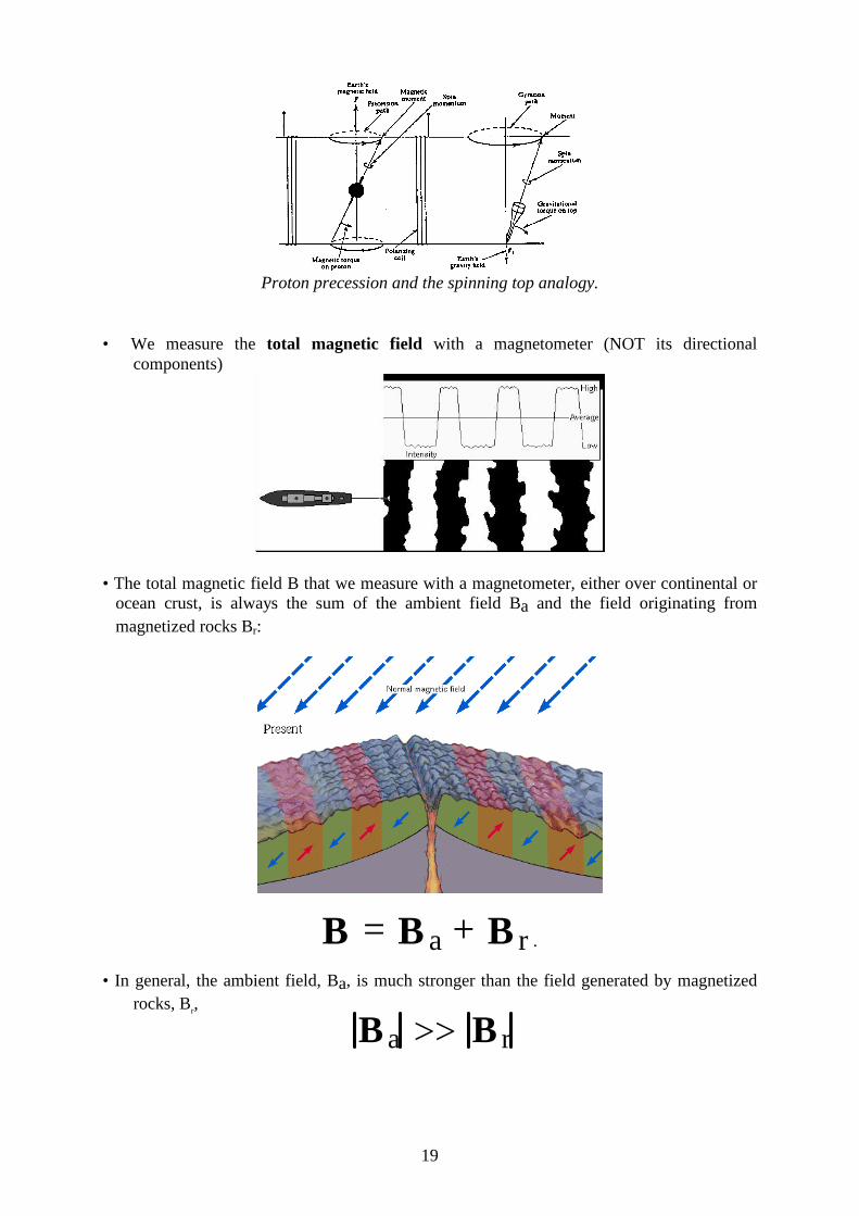
We map the oceanic magnetic field by using a proton precession magnetometer. It was invented by Packard and Varian, and is the most commonly used magnetometer today. It is based on the fact that nuclear magnetic moments posses a spin, which will precess about the earth's magnetic field. In the magnetometer the free-precession of hydrogen nuclei (= protons) is measured. In the absence of a magnetic field the dipole moments of protons in water are randomly oriented. In the presence of a strong magnetic field the dipoles become polarized in the direction of the field. When the field is removed the protons spin oriented around the direction of the Earth’s magnetic field for a short time, until they return to their random state. After the polarizing field has been switched off , the frequency of the spinning protons is counted. The precession frequency is proportional to the field strength. As a consequence the proton precession magnetometer produces a number of discrete measurements of the absolute field strenght by means of the proton precession frequency. The advantage of this type of magnetometer is that the orientation of the instument is not critrical.

19

Proton precession and the spinning top analogy.

• We measure the total magnetic field with a magnetometer (NOT its directional

components)

• The total magnetic field B that we measure with a magnetometer, either over continental or

ocean crust, is always the sum of the ambient field Ba and the field originating from magnetized rocks Br:

B = B a + B r . • In general, the ambient field, Ba, is much stronger than the field generated by magnetized

rocks, Br,

Ba >> B r

20

. .

sea level

sea floor

Earth's magnetic field

negativeanomaly

positiveanomaly

SN

remanently magnetizedcrustal layer

block of normal polarity

Field from magnetizedcrustal block

≈ 50

0 m

• In order to reduce the field to that originating from the rocks, we remove the dipole field. • The amplitude of the measured anomalies is usually of the order of a few hundred

nannoTeslas, or about 1% of the dipole field. • The average thickness of the main magnetized layer in the upper ocean crust is about 500

m. Intensity of magnetization in the upper 500 m is largest because of the more rapid cooling, forming small magnetite grains (“single domain crystals” ).

Marine magnetic anomalies: how do they work?

Introduction

Magnetic stripes offshore California

The discovery of magnetic striping naturally prompted more questions: How does the magnetic striping pattern form? And why are the stripes symmetrical around the crests of the

21

mid-ocean ridges? These questions could not be answered without also knowing the significance of these ridges. In 1961, scientists began to theorize that mid-ocean ridges mark structurally weak zones where the ocean floor was being ripped in two lengthwise along the ridge crest. New magma from deep within the Earth rises easily through these weak zones and eventually erupts along the crest of the ridges to create new oceanic crust. In 1963, F. Vine and D.H. Matthews reasoned that, as basaltic magma rises to form new ocean floor at a mid-ocean spreading center, it records the polarity of the magnetic field existing at the time magma crystalli zed. As spreading pulls the new oceanic crust apart, stripes of approximately the same size should be carried away from the ridge on each side (Fig. 5). Basaltic magma forming at mid-ocean ridges serves as a kind of "tape recorder", recording the Earth's magnetic field as it reverses through time. If this idea is correct, alternating stripes of normal and reversed polarity should be arranged symmetrically about mid-ocean spreading centers. The discovery of such magnetic stripes provided powerful evidence that sea-floor spreading occurs. This process, later called seafloor spreading, operating over many milli ons of years has built the 50,000 km-long system of mid-ocean ridges. This hypothesis was supported by several li nes of evidence: (1) at or near the crest of the ridge, the rocks are very young, and they become progressively

older away from the ridge crest; (2) the youngest rocks at the ridge crest always have present-day (normal) polarity; and (3) stripes of rock parallel to the ridge crest alternated in magnetic polarity (normal-reversed-

normal, etc.), suggesting that the Earth's magnetic field has flip-flopped many times. By explaining both the zebralike magnetic striping and the construction of the mid-ocean ridge system, the seafloor spreading hypothesis quickly gained converts and represented another major advance in the development of the plate-tectonics theory. Furthermore, the oceanic crust now came to be appreciated as a natural "tape recording" of the history of the reversals in the Earth's magnetic field.

Shape and intensity of seafloor magnetic anomalies

The shape and intensity of magnetic anomalies depends on:

(1) the segmentation of the mid-ocean ridge by fracture zones (i.e. length of magnetized blocks along-axis),

(2) spreading velocity (length of blocks across-axis). Fast spreading causes relatively longer

blocks to form than slow spreading. (3) frequency of polarity reversals (length of blocks across-axis), and (4) the direction of magnetization in a given block. When both the crustal magnetization

and geomagnetic field vectors are steep (i.e. in the vicinity of the magnetic pole), the normal blocks cause positive anomalies. However, near the equator, east-west striking

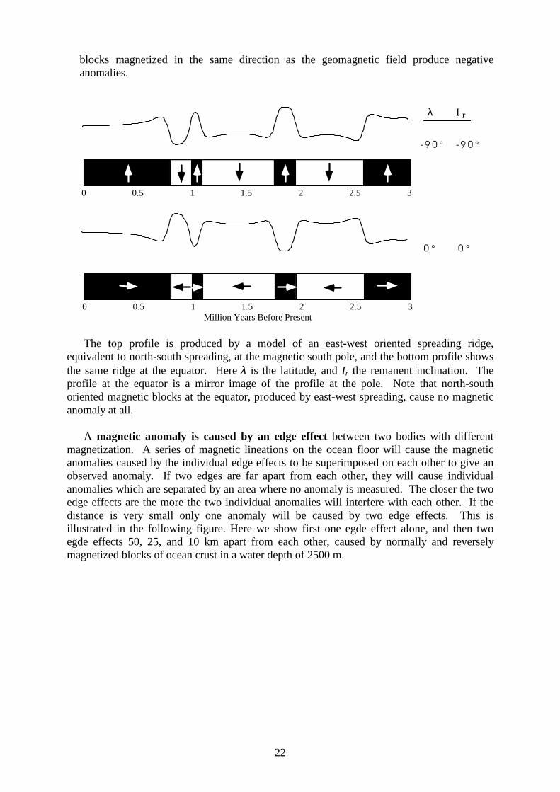
22

blocks magnetized in the same direction as the geomagnetic field produce negative anomalies.

0 0.5 1 1.5 2 2.5 3 Million Years Before Present

0 0.5 1 1.5 2 2.5 3

I rλ

- 9 0 ° - 9 0 °

0 ° 0 °

The top profile is produced by a model of an east-west oriented spreading ridge,

equivalent to north-south spreading, at the magnetic south pole, and the bottom profile shows the same ridge at the equator. Here λ is the latitude, and Ir the remanent inclination. The profile at the equator is a mirror image of the profile at the pole. Note that north-south oriented magnetic blocks at the equator, produced by east-west spreading, cause no magnetic anomaly at all.

A magnetic anomaly is caused by an edge effect between two bodies with different

magnetization. A series of magnetic lineations on the ocean floor will cause the magnetic anomalies caused by the individual edge effects to be superimposed on each other to give an observed anomaly. If two edges are far apart from each other, they will cause individual anomalies which are separated by an area where no anomaly is measured. The closer the two edge effects are the more the two individual anomalies will interfere with each other. If the distance is very small only one anomaly will be caused by two edge effects. This is illustrated in the following figure. Here we show first one egde effect alone, and then two egde effects 50, 25, and 10 km apart from each other, caused by normally and reversely magnetized blocks of ocean crust in a water depth of 2500 m.

23

0 50 100 150 200

Distance [km]

2500 m

500 m

A profound consequence of seafloor spreading is that new crust was, and is now, being continually created along the oceanic ridges. This idea found great favor with some scientists who claimed that the shifting of the continents can be simply explained by a large increase in size of the Earth since its formation. However, this so-called "expanding Earth" hypothesis was unsatisfactory because its supporters could offer no convincing geologic mechanism to produce such a huge, sudden expansion. Most geologists believe that the Earth has changed littl e, if at all , in size since its formation 4.6 billi on years ago, raising a key question: how can new crust be continuously added along the oceanic ridges without increasing the size of the Earth? This question particularly intrigued Harry H. Hess, a Princeton University geologist and a Naval Reserve Rear Admiral, and Robert S. Dietz, a scientist with the U.S. Coast and Geodetic Survey who first coined the term seafloor spreading. Dietz and Hess were among the small handful who really understood the broad implications of sea floor spreading. If the Earth's crust was expanding along the oceanic ridges, Hess reasoned, it must be shrinking elsewhere. He suggested that new oceanic crust continuously spread away from the ridges in a conveyor belt-li ke motion. Many milli ons of years later, the oceanic crust eventually descends

24

into the oceanic trenches -- very deep, narrow canyons along the rim of the Pacific Ocean basin. According to Hess, the Atlantic Ocean was expanding while the Pacific Ocean was shrinking. As old oceanic crust was consumed in the trenches, new magma rose and erupted along the spreading ridges to form new crust. In effect, the ocean basins were perpetually being "recycled," with the creation of new crust and the destruction of old oceanic lithosphere occurring simultaneously. Thus, Hess' ideas neatly explained why the Earth does not get bigger with sea floor spreading, why there is so littl e sediment accumulation on the ocean floor, and why oceanic rocks are much younger than continental rocks.

Deep Sea Drilling

Additional evidence of seafloor spreading came from an unexpected source: petroleum exploration. In the years following World War II , continental oil reserves were being depleted rapidly and the search for offshore oil was on. To conduct offshore exploration, oil companies built ships equipped with a special drilli ng rig and the capacity to carry many kilometers of drill pipe. This basic idea later was adapted in constructing a research vessel, named the Glomar Challenger, designed specifically for marine geology studies, including the collection of drill -core samples from the deep ocean floor. In 1968, the vessel embarked on a year-long scientific expedition, criss-crossing the Mid-Atlantic Ridge between South America and Africa and drilli ng core samples at specific locations. • the third leg of the Deep Sea Drilli ng Program (DSDP) drill ed a number of holes in the

South Atlantic at right angles to the mid-Atlantic Ridge to test the SFS hypothesis. –> the oldest sediments overlying the ocean crust were drill ed and dated paleontologically –> the agreement with ages predicted from magnetostratigraphy was excellent

Concentration of earthquakes

During the 20th century, improvements in seismic instrumentation and greater use of earthquake-recording instruments (seismographs) worldwide enabled scientists to learn that earthquakes tend to be concentrated in certain areas, most notably along the oceanic trenches and spreading ridges. By the late 1920s, seismologists were beginning to identify several prominent earthquake zones parallel to the trenches that typically were inclined 40-60° from the horizontal and extended several hundred kilometers into the Earth. These zones later became known as Wadati-Benioff zones, or simply Benioff zones, in honor of the seismologists who first recognized them, Kiyoo Wadati of Japan and Hugo Benioff of the United States. The study of global seismicity greatly advanced in the 1960s with the establishment of the Worldwide Standardized Seismograph Network (WWSSN) to monitor the compliance of the 1963 treaty banning above-ground testing of nuclear weapons. The much-improved data from the WWSSN instruments allowed seismologists to map precisely the zones of earthquake concentration worldwide, as shown below.

25

Earthquakes in subduction zones. In subduction zones, earthquake foci vary from shallow, near the trench, to deep, farther away from the trench in the direction of plate subduction. This drawing shows earthquakes that occurred beneath the Tonga Trench in the Pacific Ocean, over a period of several months. Earthquakes in this region are generated by the downward movement of the Pacific Plate. Zones of shallow-to-deep earthquakes like this one are also called Benioff zones.

Marine gravity anomalies from satellite altimetry

Satellite radar altimetry has revolutionized our knowledge of the topography of oceanic basement, and helped greatly to construct better plate tectonic models through geologic time. Radar altimetry works by measuring the distance between the satellite and the sea surface by radar (below). These data are used to provide a geoid map. The geoid is an equipotential field.

26

From these geoid anomalies we can derive anomalies in the gravity field. Gravity anomalies are deviations of the gravity field of that caused by the best elli psoid approximation of the Earth (i.e. the Earth’s shape can roughly be described by an elli psoid, but not quite – there are many deviations. Shor t wavelength mar ine gravity anomalies are mostly caused by oceanic basement topography, such as fracture zones, seamounts, r idgs and trenches (see figure below).

The theory of plate tectonics

Introduction

The concept of sea floor spreading was or iginally proposed by Hess (1962) and Dietz (1961), who suggested that new sea floor is created at mid-ocean r idges and spreads away form them as it ages. I t must be stressed that this idea is significantly different from the proposal by Wegener (1924) that continents “ dr ift” on a passive ocean floor .

27

A major contribution came from Wilson (1965), who developed the concept of plates and transform faults. He suggested that

(1) the active mobile belts on the surface of the Earth are not isolated but continuous (2) these mobile belts, marked by active epicenters, separate the Earth into a rigid set of plates (3) these active mobile belts consist of (a) r idges where plate is created, (b) trenches where plate is destroyed. and (c) transform faults, which connect the other two belts to each other.

Plate tectonic concepts:

(1) Continuity of plate boundaries

Plate boundaries are outlined by active Earthquake epicenters. Morgan (1968) separated the world into 10 plates. Today, we know that the actual number of plates is much larger. All major plates are surrounded by spreading centers, subduction zones, and transform faults.

(2) Rigidity

The concept of internal rigidity of tectonic plates together with Euler's Theorem allows us to model the relative motion of plates quantitatively.

(3) Relative motion

All plates can be viewed as rigid caps on the surface of a sphere. The motion of a plate can be described by a rotation about a vir tual axis which passes through the center of the sphere (Euler's Theorem). In terms of the Earth this implies that motions of plates can be described by an angular velocity vector originating at the center of the globe. The most widespread parametrization of such a vector is using latitude, longitude, describing the location where the rotation axis cuts the surface of the Earth, and a rotation rate that corresponds to the magnitude of the angular velocity (degrees per m.y. or microradians per year). The latitude and longitude of the angular velocity vector are called the “ Euler pole”.

Because angular velocities behave as vectors, the motion of a plate can be expressed as a

rotation ω� = ω k, where ω� is the angular velocity, k is a unit vector along the rotation axis, ω the rotation rate. The motion of individual plates can be described by an absolute motion angular velocity. The motion between two plates, which have different absolute motion poles, can be expressed by an angular velocity of relative motion. Plate tectonic theory was developed by determining relative motion between plates, which - in general - is easier to measure than their absolute motions.

28

29

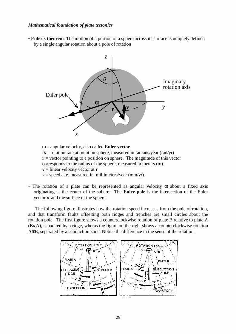
Mathematical foundation of plate tectonics

• Euler's theorem: The motion of a portion of a sphere across its surface is uniquely defined

by a single angular rotation about a pole of rotation

z

x

yr v

θ

ω�

Imaginaryrotation axis

Euler pole

ω� = angular velocity, also called Euler vector ω = rotation rate at point on sphere, measured in radians/year (rad/yr) r = vector pointing to a position on sphere. The magnitude of this vector corresponds to the radius of the sphere, measured in meters (m). v = linear velocity vector at r v = speed at r , measured in millimeters/year (mm/yr).

• The rotation of a plate can be represented as angular velocity ω� about a fixed axis

originating at the center of the sphere. The Euler pole is the intersection of the Euler vector ω� and the surface of the sphere. The following figure ill ustrates how the rotation speed increases from the pole of rotation,

and that transform faults offsetting both ridges and trenches are small circles about the rotation pole. The first figure shows a counterclockwise rotation of plate B relative to plate A (Bω� A), separated by a ridge, wheras the figure on the right shows a counterclockwise rotation Aω� B, separated by a subduction zone. Notice the difference in the sense of the rotation.

B ω� A Aω� B

PLATE B

PLATE B PLATE A

PLATE A

30

Formal hypothesis of plate tectonics

• These concepts lead directly to the formal hypothesis of plate tectonics: The earth is envisioned as an interlocking internally rigid set of plates in constant motion. These plates are rigid except at plate boundaries whcih are lines between contiguous plates. The relative motion between plates gives rise to earthquakes. These earthquakes define the plate boundaries.

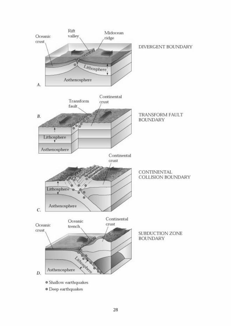
Plate boundaries There are three types of plate boundaries: Divergent boundaries -- where new crust is generated as the plates diverge. Convergent boundaries -- where crust is destroyed as one plate dives under another. Transform boundaries -- where crust is neither produced nor destroyed as the plates slide horizontally past each other.

Types of plate boundaries

Divergent boundaries

Divergent boundaries occur along spreading centers where plates are moving apart and new crust is created by magma pushing up from the mantle. Picture two giant conveyor belts, facing each other but slowly moving in opposite directions as they transport newly formed oceanic crust away from the ridge crest. Perhaps the best known of the divergent boundaries is the Mid-Atlantic Ridge. This submerged mountain range, which extends from the Arctic Ocean to beyond the southern tip of Africa, is but one segment of the global mid-ocean ridge system that encircles the Earth. The rate of spreading along the Mid-Atlantic Ridge averages about 2.5 centimeters per year (cm/yr), or 25 km in a milli on years. This rate may seem slow by human standards, but

31

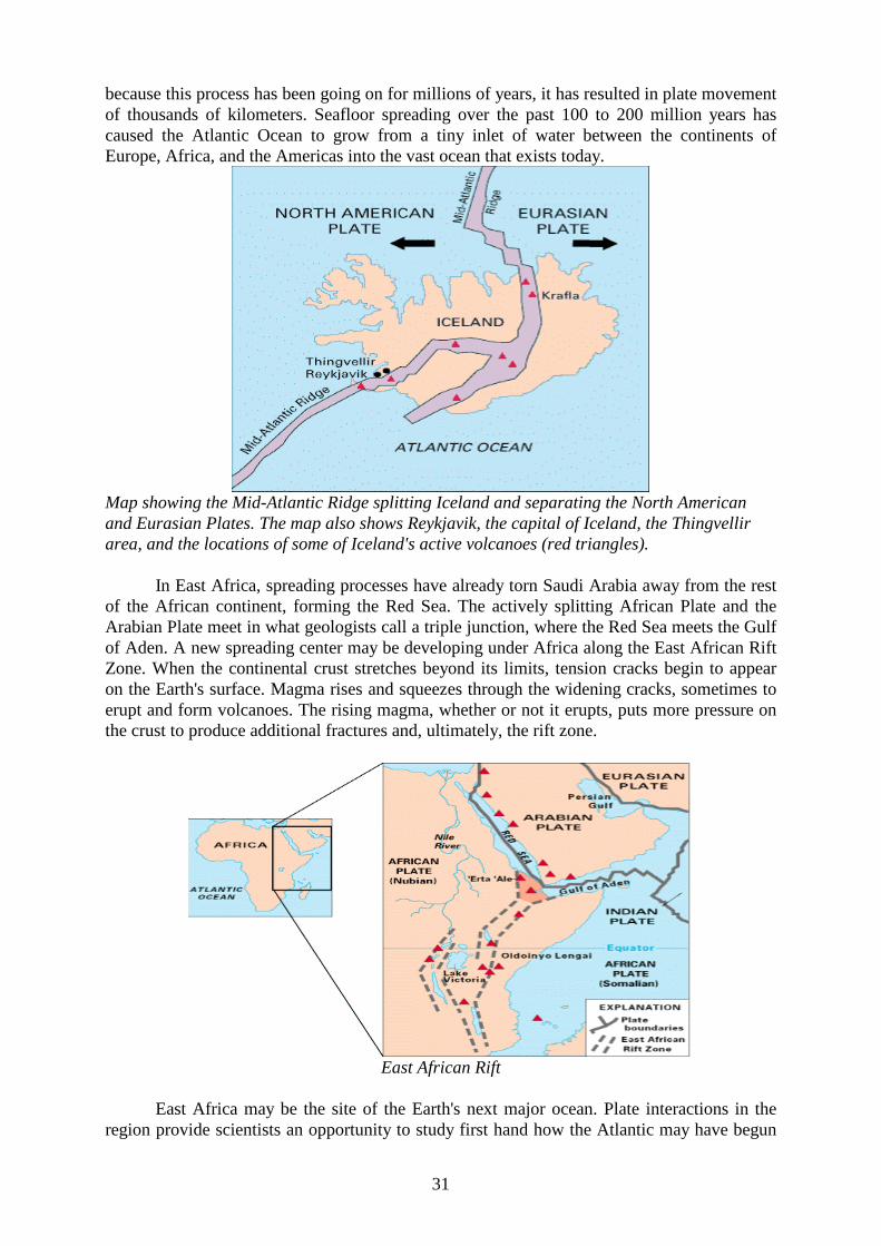
because this process has been going on for milli ons of years, it has resulted in plate movement of thousands of kilometers. Seafloor spreading over the past 100 to 200 milli on years has caused the Atlantic Ocean to grow from a tiny inlet of water between the continents of Europe, Africa, and the Americas into the vast ocean that exists today.

Map showing the Mid-Atlantic Ridge splitti ng Iceland and separating the North American and Eurasian Plates. The map also shows Reykjavik, the capital of Iceland, the Thingvelli r area, and the locations of some of Iceland's active volcanoes (red triangles). In East Africa, spreading processes have already torn Saudi Arabia away from the rest of the African continent, forming the Red Sea. The actively splitti ng African Plate and the Arabian Plate meet in what geologists call a triple junction, where the Red Sea meets the Gulf of Aden. A new spreading center may be developing under Africa along the East African Rift Zone. When the continental crust stretches beyond its limits, tension cracks begin to appear on the Earth's surface. Magma rises and squeezes through the widening cracks, sometimes to erupt and form volcanoes. The rising magma, whether or not it erupts, puts more pressure on the crust to produce additional fractures and, ultimately, the rift zone.

East African Rift

East Africa may be the site of the Earth's next major ocean. Plate interactions in the region provide scientists an opportunity to study first hand how the Atlantic may have begun

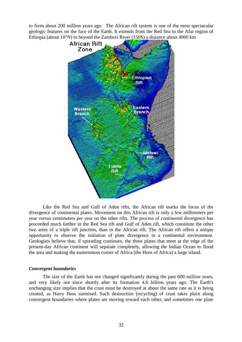
32

to form about 200 milli on years ago. The African rift system is one of the most spectacular geologic features on the face of the Earth. It extends from the Red Sea in the Afar region of Ethiopia (about 10°N) to beyond the Zambezi River (150S) a distance about 4000 km

Like the Red Sea and Gulf of Aden rifts, the African rift marks the locus of the divergence of continental plates. Movement on this African rift is only a few millimeters per year versus centimeters per year on the other rifts. The process of continental divergence has proceeded much farther in the Red Sea rift and Gulf of Aden rift, which constitute the other two arms of a triple rift junction, than in the African rift. The African rift offers a unique opportunity to observe the initiation of plate divergence in a continental environment. Geologists believe that, if spreading continues, the three plates that meet at the edge of the present-day African continent will separate completely, allowing the Indian Ocean to flood the area and making the easternmost corner of Africa (the Horn of Africa) a large island.

Convergent boundaries

The size of the Earth has not changed significantly during the past 600 milli on years, and very likely not since shortly after its formation 4.6 billi on years ago. The Earth's unchanging size implies that the crust must be destroyed at about the same rate as it is being created, as Harry Hess surmised. Such destruction (recycling) of crust takes place along convergent boundaries where plates are moving toward each other, and sometimes one plate

33

sinks (is subducted) under another. The location where sinking of a plate occurs is called a subduction zone. The type of convergence -- called by some a very slow "collision" -- that takes place between plates depends on the kind of lithosphere involved. Convergence can occur between an oceanic and a largely continental plate, or between two largely oceanic plates, or between two largely continental plates.

Oceanic-continental convergence

Along the rim of the Pacific, we find a number of long narrow, curving trenches thousands of kilometers long and 8 to 10 km deep cutting into the ocean floor.

“ Ring of fire” along the Pacific rim created by subduction

Trenches are the deepest parts of the ocean floor and are created by subduction.

34

Profile through oceanic-continental subduction zone off South America

Plate convergence vectors between the Nazca and the Pacific Plate

Off the coast of South America along the Peru-Chile trench, the oceanic Nazca Plate is pushing into and being subducted under the continental part of the South American Plate. In turn, the overriding South American Plate is being lifted up, creating the Andes mountains.

35

Strong, destructive earthquakes and the rapid upli ft of mountain ranges are common in this region.

Even though the Nazca Plate as a whole is sinking smoothly and continuously into the trench, the deepest part of the subducting plate breaks into smaller pieces that become locked in place for long periods of time before suddenly moving to generate large earthquakes. Such earthquakes are often accompanied by upli ft of the land by as much as a few meters.

On 9 June 1994, a magnitude-8.3 earthquake struck about 320 km northeast of La Paz, Bolivia, at a depth of 636 km. This earthquake, within the subduction zone between the Nazca Plate and the South American Plate, was one of deepest and largest subduction earthquakes recorded in South America. Fortunately, even though this powerful earthquake was felt as far away as Minnesota and Toronto, Canada, it caused no major damage because of its great depth. Oceanic-continental convergence also sustains many of the Earth's active volcanoes, such as those in the Andes and the Cascade Range in the Pacific Northwest.

The eruptive activity is clearly associated with subduction, but scientists vigorously debate the possible sources of magma: Is magma generated by the partial melting of the subducted oceanic slab, or the overlying continental lit hosphere, or both?

Oceanic-oceanic convergence

As with oceanic-continental convergence, when two oceanic plates converge, one is usually subducted under the other, and in the process a trench is formed. The Marianas Trench (paralleling the Mariana Islands), for example, marks where the fast-moving Pacific Plate converges against the slower moving Phili ppine Plate. The Challenger Deep, at the

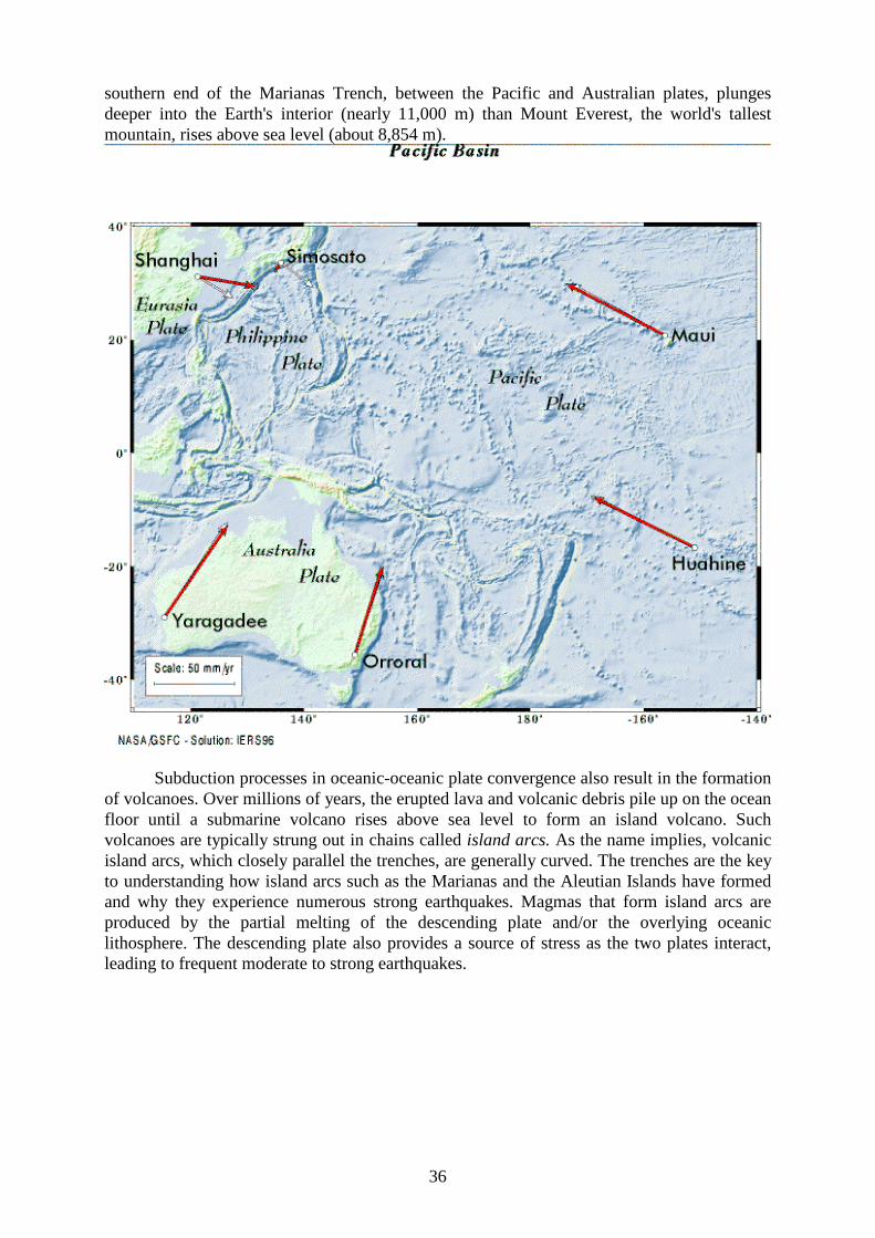
36

southern end of the Marianas Trench, between the Pacific and Australian plates, plunges deeper into the Earth's interior (nearly 11,000 m) than Mount Everest, the world's tallest mountain, rises above sea level (about 8,854 m).

Subduction processes in oceanic-oceanic plate convergence also result in the formation of volcanoes. Over milli ons of years, the erupted lava and volcanic debris pile up on the ocean floor until a submarine volcano rises above sea level to form an island volcano. Such volcanoes are typically strung out in chains called island arcs. As the name implies, volcanic island arcs, which closely parallel the trenches, are generally curved. The trenches are the key to understanding how island arcs such as the Marianas and the Aleutian Islands have formed and why they experience numerous strong earthquakes. Magmas that form island arcs are produced by the partial melting of the descending plate and/or the overlying oceanic lithosphere. The descending plate also provides a source of stress as the two plates interact, leading to frequent moderate to strong earthquakes.

37

Continental-continental convergence

The Himalayan mountain range dramatically demonstrates one of the most visible and spectacular consequences of plate tectonics. When two continents meet head-on, neither is subducted because the continental rocks are relatively light and, like two colliding icebergs, resist downward motion. Instead, the crust tends to buckle and be pushed upward or sideways. The collision of India into Asia 50 million years ago caused the Eurasian Plate to crumple up and override the Indian Plate. After the collision, the slow continuous convergence of the two plates over millions of years pushed up the Himalayas and the Tibetan Plateau to their present heights. Most of this growth occurred during the past 10 million years. The Himalayas, towering as high as 8,854 m above sea level, form the highest continental mountains in the world. Moreover, the neighboring Tibetan Plateau, at an average elevation of about 4,600 m, is higher than all the peaks in the Alps except for Mont Blanc and Monte Rosa, and is well above the summits of most mountains in the United States.

The collision between the Indian and Eurasian plates has pushed up the Himalayas and the Tibetan Plateau.

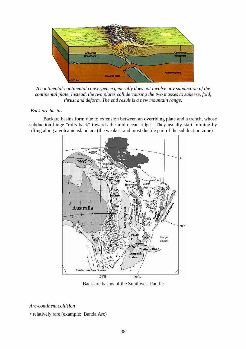
38

A continental-continental convergence generally does not involve any subduction of the continental plate. Instead, the two plates collide causing the two masses to squeeze, fold,

thrust and deform. The end result is a new mountain range.

Back arc basins

Backarc basins form due to extension between an overriding plate and a trench, whose subduction hinge "rolls back" towards the mid-ocean ridge. They usually start forming by rifting along a volcanic island arc (the weakest and most ductile part of the subduction zone)

Back-arc basins of the Southwest Pacific

Arc-continent collision

• relatively rare (example: Banda Arc)

39

• when a continent hits an island arc, the continent cannot be underthrusted because of its negative buoyancy •> slices of oceanic crust and sediments are driven into the continental margin

• when colli sion is complete, a new trench may develop

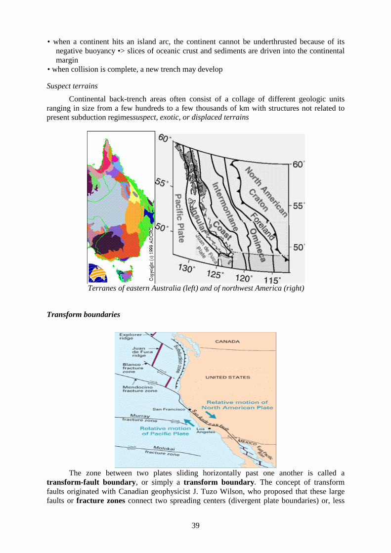
Suspect terrains

Continental back-trench areas often consist of a collage of different geologic units ranging in size from a few hundreds to a few thousands of km with structures not related to present subduction regimessuspect, exotic, or displaced terrains

Terranes of eastern Australia (left) and of northwest America (right)

Transform boundaries

The zone between two plates sliding horizontally past one another is called a transform-fault boundary, or simply a transform boundary. The concept of transform faults originated with Canadian geophysicist J. Tuzo Wilson, who proposed that these large faults or fracture zones connect two spreading centers (divergent plate boundaries) or, less

40

commonly, trenches (convergent plate boundaries). Most transform faults are found on the ocean floor. They commonly offset the active spreading ridges, producing zig-zag plate margins, and are generally defined by shallow earthquakes. However, a few occur on land, for example the San Andreas fault zone in Cali fornia. This transform fault connects the East Pacific Rise, a divergent boundary to the south, with the South Gorda -- Juan de Fuca -- Explorer Ridge, another divergent boundary to the north. The San Andreas fault zone, which is about 1,300 km long and in places tens of kilometers wide, slices through two thirds of the length of Cali fornia. Along it, the Pacific Plate has been grinding horizontally past the North American Plate for 10 milli on years, at an average rate of about 5 cm/yr. Land on the west side of the fault zone (on the Pacific Plate) is moving in a northwesterly direction relative to the land on the east side of the fault zone (on the North American Plate). Oceanic fracture zones are ocean-floor valleys that horizontally offset spreading ridges; some of these zones are hundreds to thousands of kilometers long and as much as 8 km deep. Examples of these large scars include the Clarion, Molokai, and Pioneer fracture zones in the Northeast Pacific off the coast of Cali fornia and Mexico. These zones are presently inactive, but the offsets of the patterns of magnetic striping provide evidence of their previous transform-fault activity. (1) All transform faults are small circles about the pole of rotation (2) The seafloor spreading rate v increases as the sine of the distance from the rotation pole

v = w rsinq (r= radius of the earth, ω =angular velocity, q=distance to the rotaion pole)

The relative velocity between two plates is zero at the rotation pole and has a maximum value at the 90° from the rotation pole Transform motion is called right-lateral when something attached to the plate on the other side of the fault appears to move to the right as seen from where you are standing on this side of the fault. If the object appears to move to the left, the motion is called left-lateral. If you were to cross to the other side of the fault, in order to face this side, you would have to turn around, and so the relative motion would appear the same. As a result, whether a fault is right- or left-lateral does not depend on which side of the fault you are on.

41

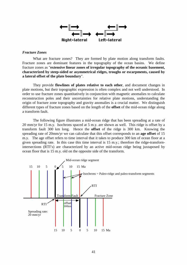
Fracture Zones

What are fracture zones? They are formed by plate motion along transform faults. Fracture zones are dominant features in the topography of the ocean basins. We define fracture zones as "extensive linear zones of irregular topography of the oceanic basement, characterized by steep-sided or asymmetrical ridges, troughs or escarpments, caused by a lateral offset of the plate boundary". They provide flowlines of plates relative to each other, and document changes in plate motions, but their topographic expression is often complex and not well understood. In order to use fracture zones quantitatively in conjunction with magnetic anomalies to calculate reconstruction poles and their uncertainties for relative plate motions, understanding the origin of fracture zone topography and gravity anomalies is a crucial matter. We distinguish different types of fracture zones based on the length of the offset of the mid-ocean ridge along a transform fault. The following figure ill ustrates a mid-ocean ridge that has been spreading at a rate of 20 mm/yr for 15 m.y. Isochrons spaced at 5 m.y. are shown as well . This ridge is offset by a transform fault 300 km long. Hence the offset of the ridge is 300 km. Knowing the spreading rate of 20mm/yr we can calculate that this offset corresponds to an age offset of 15 m.y. The age offset refers to time interval that it takes to produce 300 km of ocean floor at a given spreading rate. In this case this time interval is 15 m.y.; therefore the ridge-transforn-intersections (RTI’s) are characterized by an active mid-ocean ridge being juxtaposed by ocean floor that is 15 m.y. old on the opposite side of the transform.

Mid-ocean ridge segment

Fracture Zone

offset

Transform Fault

5 5 10 151015 Ma0

300km

Spreading rate:20 mm/yr

Isochrons = Paleo-ridge and paleo-transform segments

RTI

RTI

5 5 10 151015 Ma0

42

Based on the length of the ridge offset, we distinguish 3 classes of fracture zone offsets: small, medium, and large. Small-offset fracture zones have offsets less than about 30 km (age offset ~2.0 m.y. for slow spreading) and dominantly represent the off-axis continuations of non-transform offsets of the mid-ocean ridge. All discontinuities of the Mid-Atlantic Ridge with offsets less than 30 km mapped to date fall in the category of non-transform offsets. Medium-offset fracture zones, defined by offsets of 30-200 km (~2 m.y. for slow spreading), are the off-axis traces of transform faults that and have a well-developed strike-slip valley. Examples for Atlantic medium-offset fracture zones are the Oceanographer, Hayes, Atlantis, and Kane fracture zones.

Pitman Fracture Zone in the South Pacific. (a) topography, (b) magnetic anomalies (S. Cande) Large-offset fracture zones have offsets of several hundreds of kilometers. In fast spreading regimes their primary characteristic is a depth-age step, which develops as a function of their large age-offsets. In slow spreading regimes they have complex morphologies that combine a depth/age step (typical for Pacific type fracture zones) with rugged topography and/or the presence of a central valley. For instance the Romanche Fracture Zone is characterized by a dominant depth/age step modified by large amplitude topography. Another morphological element often observed at North Atlantic medium and large-offset fracture zones is an asymmetry in their cross section, expressed as a high wall (often termed transverse ridge) on the old side of fracture zones.

43

Large-offset fracture zones in the Pacific Ocean

Fracture zone model

Along fracture zones, lithosphere of different ages is juxtaposed:

This creates a "steplike" topography, as older ocean floor is colder and deeper and compared with that of young, hot ocean floor.

Triple junctions

Introduction

• a triple junction is a place where 3 plates come into contact. • only RRR (ridge-ridge-ridge) triple junctions are stable for any orientation of the ridges • the stabilit y of a triple junction can be determined by constructing "velocity triangles" • consider a ridge-ridge-ridge (RRR) triple junction:

44

vAB

vBC

vCA

A B

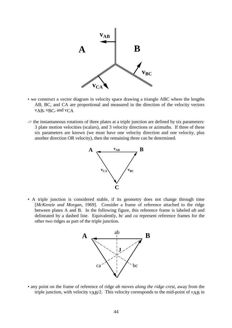
• we construct a vector diagram in velocity space drawing a triangle ABC where the lengths

AB, BC, and CA are proportional and measured in the direction of the velocity vectors vAB, vBC, and vCA

-> the instantaneous rotations of three plates at a triple junction are defined by six parameters:

3 plate motion velocities (scalars), and 3 velocity directions or azimuths. If three of these six parameters are known (we must have one velocity direction and one velocity, plus another direction OR velocity), then the remaining three can be determined.

A B

C

vAB

vBCvCA

• A triple junction is considered stable, if its geometry does not change through time

[McKenzie and Morgan, 1969]. Consider a frame of reference attached to the ridge between plates A and B. In the following figure, this reference frame is labeled ab and delineated by a dashed line. Equivalently, bc and ca represent reference frames for the other two ridges as part of the triple junction.

A Bab

bcca

J

• any point on the frame of reference of ridge ab moves along the ridge crest, away from the

triple junction, with velocity vAB/2. This velocity corresponds to the mid-point of vAB in

45

velocity space. In other words, any point on the reference frame ab is moving parallel to the ridge axis, and along the mid-point between A and B.

• on the earth there are many triple junctions, but no 4 plate boundaries • most major triple junctions are stable as they develop through time with the same geometry. • Triple junctions are classified by the type of boundaries which meet at the triple junction. A

few important end members of triple junction types are: (1) Ridge, ridge, ridge triple junction (RRR) (2) Ridge, transform fault, transform fault junction (RFF) (3) Trench, trench, trench junction (TTT)

Summary

(1) All transform faults are small circles about the pole of rotation representing the motion between the two plates.

(2) The velocity of separation of two plates increases as the sine of the colatitude (latidude •

90� � DZD� IUR� WK � URWDWL ������ OH� (3) At a triple junction the velocity vectors sum to zero. (4) Taking any path over the surface of the earth beginning and ending on the same plate, the

angular velocity vectors sum to zero. There are 16 different triple junction types, the most common of which are shown below.

46

Plate-boundary zones

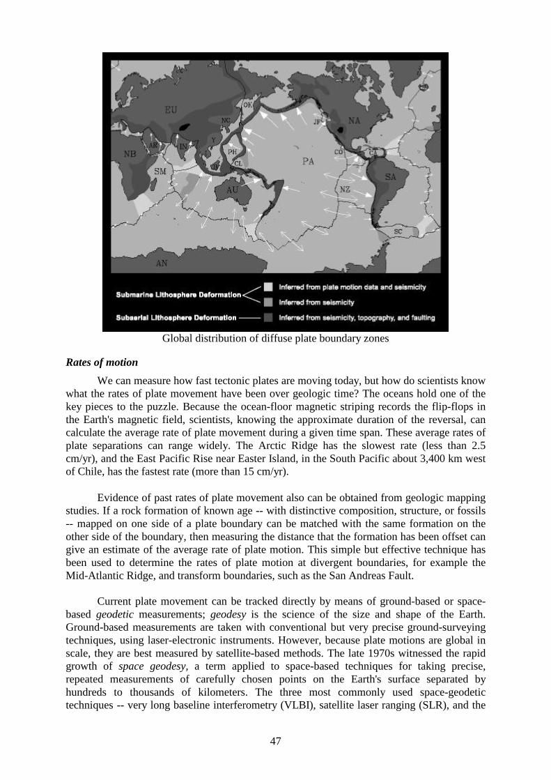
Not all plate boundaries are as simple as the main types discussed above. In some regions, the boundaries are not well defined because the plate-movement deformation occurring there extends over a broad belt (called a plate-boundary zone). One of these zones marks the Mediterranean-Alpine region between the Eurasian and African Plates, within which several smaller fragments of plates (microplates) have been recognized. Because plate-boundary zones involve at least two large plates and one or more microplates caught up between them, they tend to have complicated geological structures and earthquake patterns.

47

Global distribution of diffuse plate boundary zones

Rates of motion

We can measure how fast tectonic plates are moving today, but how do scientists know what the rates of plate movement have been over geologic time? The oceans hold one of the key pieces to the puzzle. Because the ocean-floor magnetic striping records the flip-flops in the Earth's magnetic field, scientists, knowing the approximate duration of the reversal, can calculate the average rate of plate movement during a given time span. These average rates of plate separations can range widely. The Arctic Ridge has the slowest rate (less than 2.5 cm/yr), and the East Pacific Rise near Easter Island, in the South Pacific about 3,400 km west of Chile, has the fastest rate (more than 15 cm/yr). Evidence of past rates of plate movement also can be obtained from geologic mapping studies. If a rock formation of known age -- with distinctive composition, structure, or fossils -- mapped on one side of a plate boundary can be matched with the same formation on the other side of the boundary, then measuring the distance that the formation has been offset can give an estimate of the average rate of plate motion. This simple but effective technique has been used to determine the rates of plate motion at divergent boundaries, for example the Mid-Atlantic Ridge, and transform boundaries, such as the San Andreas Fault. Current plate movement can be tracked directly by means of ground-based or space-based geodetic measurements; geodesy is the science of the size and shape of the Earth. Ground-based measurements are taken with conventional but very precise ground-surveying techniques, using laser-electronic instruments. However, because plate motions are global in scale, they are best measured by satellit e-based methods. The late 1970s witnessed the rapid growth of space geodesy, a term applied to space-based techniques for taking precise, repeated measurements of carefully chosen points on the Earth's surface separated by hundreds to thousands of kilometers. The three most commonly used space-geodetic techniques -- very long baseline interferometry (VLBI), satellit e laser ranging (SLR), and the

48

Global Positioning System (GPS) -- are based on technologies developed for military and aerospace research, notably radio astronomy and satellit e tracking. Among the three techniques, to date the GPS has been the most useful for studying the Earth's crustal movements. Twenty-one satellit es are currently in orbit 20,000 km above the Earth as part of the NavStar system of the U.S. Department of Defense. These satellit es continuously transmit radio signals back to Earth. To determine its precise position on Earth (longitude, latitude, elevation), each GPS ground site must simultaneously receive signals from at least four satellit es, recording the exact time and location of each satellit e when its signal was received.

Present day plate motions

By repeatedly measuring distances between specific points, geologists can determine if there has been active movement along faults or between plates. The separations between GPS sites are already being measured regularly around the Pacific basin. By monitoring the interaction between the Pacific Plate and the surrounding, largely continental plates, scientists hope to learn more about the events building up to earthquakes and volcanic eruptions in the circum-Pacific Ring of Fire. Space-geodetic data have already confirmed that the rates and direction of plate movement, averaged over several years, compare well with rates and direction of plate movement averaged over milli ons of years.

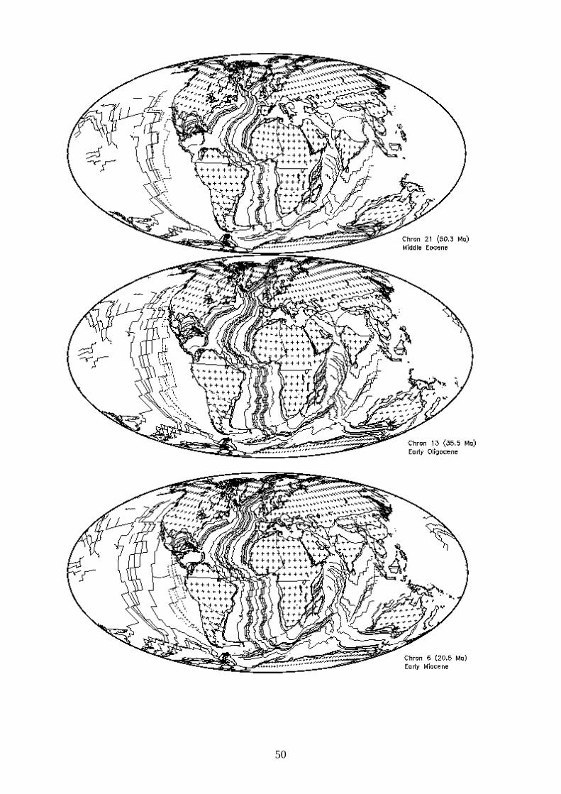
Plate motions since the Late Jurassic

Magnetic anomalies and fractures zones in the ocean basins have been used to reconstruct the major plates since the Jurassic. The following figures show a series of snapshots, including oceanic isochons, i.e. lines of equal age in the ocean basins. Each isochron corresponds to a past location of a mid-ocean ridge.

49

50

51

Hotspots

Hawaii

The vast majority of earthquakes and volcanic eruptions occur near plate boundaries, but there are some exceptions. For example, the Hawaiian Islands, which are entirely of volcanic origin, have formed in the middle of the Pacific Ocean more than 3,200 km from the nearest plate boundary. How do the Hawaiian Islands and other volcanoes that form in the interior of plates fit into the plate-tectonics picture?

52

Global distribution of hotspots

A widely used method of reconstructing plates relative to a fixed mesosphere utili zes linear chains of volcanoes that display age progression and are thought to be caused by focused spots of melting in the upper mantle.

Plume theory

In 1963, J. Tuzo Wilson, the Canadian geophysicist who discovered transform faults, came up with an ingenious idea that became known as the "hotspot" theory. Wilson noted that in certain locations around the world, such as Hawaii , volcanism has been active for very long periods of time. This could only happen, he reasoned, if relatively small , long-lasting, and exceptionally hot regions -- called hotspots -- existed below the plates that would provide localized sources of high heat energy (thermal plumes) to sustain volcanism.

Oceanic crust

Lithosphericmantle

6-9 km

10-60 km

H o t

C o ld

200-400 km

Oceanic flood basalts

Mantle plume

Upwelli ng mantle plumes are throught to form either at the core-mantle boundary (2900 km depth) or the boundary between the lower and upper mantle (670 km depth). One theory suggests that a “plume head” develops, above a “plume stem”.

53

Iceland plume stem as imaged with seismic tomography

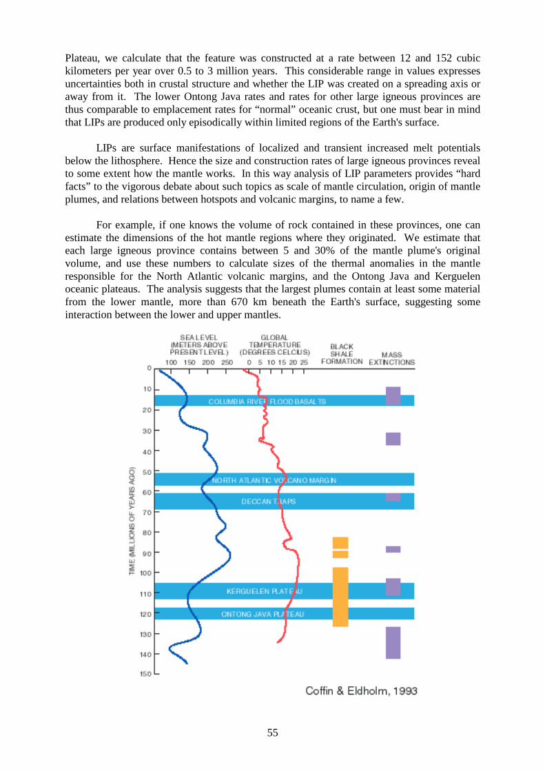
Large Igneous Provinces (LIPS)

Volcanic eruptions, such as that in 1991 of Mt. Pinatubo in the Phili ppines, can severely damage the local environment. Yet such events pale in comparison to the huge convulsions of magmatic activity during the formation of large igneous provinces, or LIPs. Today LIPs are found both on land, as continental flood basalts, and under the sea, primarily as oceanic plateaus in the middle of oceans, and as volcanic passive margins along the edges of continents.

Global distribution of large igneous provinces (compiled by M. Coff in)

In fact, the two largest provinces, the Ontong Java and Kerguelen plateaus, now lie mostly below sea level. The construction of these two provinces, together with the volcanic passive margins between Greenland and NW Europe, not only have profound implications for the regional and global environment, but also partially reveal the workings of the mantle, that part of the Earth's interior between the outer crust and molten core. Cores obtained from oceanic plateaus and volcanic passive margins by the Deep Sea Drilli ng Project and the

54

Ocean Drilli ng Program, together with high-quality seismic reflection images, have been instrumental in allowing scientists to understand the causes and effects of large igneous provinces. While the theory of plate tectonics explains much of the geology we observe on the Earth's surface, it does not readily explain large igneous provinces. These provinces are created neither by “normal” seafloor spreading, which occurs along the mid-ocean ridge system, nor by the subduction process, where one lithospheric plate ~100 km thick slides beneath another. On a geological time scale, both processes reflect persistent phenomena while LIP formation is transient. Although large igneous province rocks resemble those created by seafloor spreading, subtle differences suggest that they arise from deeper, hotter regions of the mantle. Early on in the development of plate tectonic theory, these regions were proposed to produce “hotspots” such as Hawaii , which somehow remain anchored in the mantle while above, the lithospheric plates move horizontally. Most researchers believe that mantle hotspots account for large igneous provinces, for example by means of a “plume head” impinging on the surface of the Earth, but the details of this process are not known. How big are large igneous provinces? The volume of the biggest LIP, the Ontong Java Plateau and associated provinces in the western Pacific, would cover the contiguous United States with 5 meters of basalt. Another large igneous province, the Columbia River continental flood basalt in the Pacific Northwest, encompasses only 3% of Ontong Java's volume. Individual lava flows of this lesser province, however, can be traced for over 750 km.

Fortescue (2.7 Ga)

Coppermine (1.3 Ga)Keweenawan (1.1 Ga)

Central Australia (800 Ma)

Siberia (250 Ma)

Karoo (165 Ma)

Deccan (65 Ma)

Ethiopia (30 Ma)

Columbia River (17 Ma)

1000

100

10

103 104 105 106 107

V o l u m e ( k m3)

Ag

e (

Ma

)

North Atlantic (<60 Ma)

Pacific & Indian Oceanic Plateaux (125 & 88 Ma)

Volumes or Large igneous provinces (LIPS) through geological time

Their rapid emplacement is diff icult to comprehend. We know, for example, that the global mid-ocean ridge system has produced between 16 and 26 cubic kilometers of basaltic crust annually over the past 150 milli on years. Through dating of rocks from the Ontong Java

55

Plateau, we calculate that the feature was constructed at a rate between 12 and 152 cubic kilometers per year over 0.5 to 3 milli on years. This considerable range in values expresses uncertainties both in crustal structure and whether the LIP was created on a spreading axis or away from it. The lower Ontong Java rates and rates for other large igneous provinces are thus comparable to emplacement rates for “normal” oceanic crust, but one must bear in mind that LIPs are produced only episodically within limited regions of the Earth's surface. LIPs are surface manifestations of localized and transient increased melt potentials below the lithosphere. Hence the size and construction rates of large igneous provinces reveal to some extent how the mantle works. In this way analysis of LIP parameters provides “hard facts” to the vigorous debate about such topics as scale of mantle circulation, origin of mantle plumes, and relations between hotspots and volcanic margins, to name a few. For example, if one knows the volume of rock contained in these provinces, one can estimate the dimensions of the hot mantle regions where they originated. We estimate that each large igneous province contains between 5 and 30% of the mantle plume's original volume, and use these numbers to calculate sizes of the thermal anomalies in the mantle responsible for the North Atlantic volcanic margins, and the Ontong Java and Kerguelen oceanic plateaus. The analysis suggests that the largest plumes contain at least some material from the lower mantle, more than 670 km beneath the Earth's surface, suggesting some interaction between the lower and upper mantles.

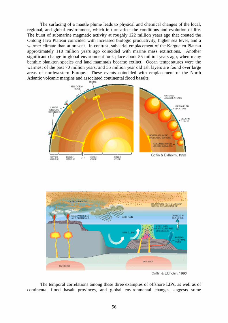
56

The surfacing of a mantle plume leads to physical and chemical changes of the local, regional, and global environment, which in turn affect the conditions and evolution of life. The burst of submarine magmatic activity at roughly 122 million years ago that created the Ontong Java Plateau coincided with increased biologic productivity, higher sea level, and a warmer climate than at present. In contrast, subaerial emplacement of the Kerguelen Plateau approximately 110 million years ago coincided with marine mass extinctions. Another significant change in global environment took place about 55 million years ago, when many benthic plankton species and land mammals became extinct. Ocean temperatures were the warmest of the past 70 million years, and 55 million year old ash layers are found over large areas of northwestern Europe. These events coincided with emplacement of the North Atlantic volcanic margins and associated continental flood basalts.

The temporal correlations among these three examples of offshore LIPs, as well as of continental flood basalt provinces, and global environmental changes suggests some

57

relationship. Although the potential forcing functions and feedback mechanisms have yet to be refined, it appears that magmatic production rates, geological setting, and the state of the environment during LIP formation are primary factors determining environmental impact. Scientific ocean drilling has only begun to scratch the surface of large igneous provinces; their crust is up to 40 km thick with a cover of numerous basalt flows exceeding 5 km. Most Deep Sea Drilling Project basement holes were quite shallow, whereas Leg 104 volcanic margin drilling by JOIDES Resolution of the Ocean Drilling Program proved the feasibility of penetrating deeply into basement rocks.

Presently, the deepest LIP hole has penetrated almost 1 km into the igneous crust, but most other holes have only penetrated a few tens of meters into the basalts. The present LIPs drilling data base is sparse, but what we have learned from the existing holes, including a recent cruise to the Kerguelen Plateau, and associated geophysical surveys is intriguing. Our current knowledge amply demonstrates that they contain crucial information about the internal behavior of the Earth and about the natural causes of global change. The Ocean Drilling Program provides a unique tool for solving such fundamental problems in geoscience.

Seamount chains

Specifically, Wilson hypothesized that the distinctive linear shape of the Hawaiian Island-Emperor Seamounts chain resulted from the Pacific Plate moving over a deep, stationary hotspot in the mantle, located beneath the present-day position of the Island of Hawaii. Heat from this hotspot produced a persistent source of magma by partly melting the overriding Pacific Plate. The magma, which is lighter than the surrounding solid rock, then rises through the mantle and crust to erupt onto the seafloor, forming an active seamount. Over time, countless eruptions cause the seamount to grow until it finally emerges above sea level to form an island volcano. Wilson suggested that continuing plate movement eventually carries the island beyond the hotspot, cutting it off from the magma source, and volcanism ceases.

58

As one island volcano becomes extinct, another develops over the hotspot, and the cycle is repeated. This process of volcano growth and death, over many milli ons of years, has left a long trail of volcanic islands and seamounts across the Pacific Ocean floor.

Age progression along Hawaiian-Emperor seamount chain

According to Wilson's hotspot theory, the volcanoes of the Hawaiian chain should get progressively older and become more eroded the farther they travel beyond the hotspot. The oldest volcanic rocks on Kauai, the northwesternmost inhabited Hawaiian island, are about 5.5 milli on years old and are deeply eroded. By comparison, on the "Big Island" of Hawaii -- southeasternmost in the chain and presumably still positioned over the hotspot -- the oldest exposed rocks are less than 0.7 milli on years old and new volcanic rock is continually being formed. Although Hawaii i s perhaps the best known hotspot, many others exist beneath the oceans and continents. More than a hundred hotspots beneath the Earth's crust have been active during the past 10 milli on years. Most of these are located under plate interiors (for example, the African Plate), but some occur near diverging plate boundaries. Some are concentrated near the mid-oceanic ridge system, such as beneath Iceland, the Azores, and the Galapagos Islands.

Absolute plate motions

Methods for reconstructing "absolute" plate motions

During the past twenty years, our knowledge of the Mesozoic and Cenozoic relative motion between the major tectonic plates has increased substantially even though "absolute" plate motions relative to a "fixed" mesosphere are still controversial. Identified marine magnetic anomalies, some as old as 165 m.y., along with seafloor tectonic lineations based on bathymetric and satellit e altimetry data accurately define relative plate motions for most of the major plates. Paleomagnetic data and hotspot traces are among the concepts that have been used to attempt to constrain the "absolute" plate motions. Paleomagnetic data can be used to determine the paleo-meridian orientation and the paleolatitude of a plate which together can be considered the paleopole for a given plate. However, since the Earth's dipole field is radially symmetric, no paleo-longitudinal information can be deduced from paleomagnetic data.

59

Seamount chains with a linear age progression (a hotspot track), can be used to restore plates to their paleopositions with the assumption that hotspots are either fixed or nearly fixed relative to each other ("fixed hotspot hypothesis"). Molnar and Stock (1987) showed though, that during the Tertiary, the Hawaiian hotspot moved with an average velocity of 10-20 mm/yr relative to the Iceland hotspot and to hotspots beneath the African and Indian plates. Numerous paleomagnetic datasets and models for the "absolute" motions of the North American, African and Eurasian plates during the Mesozoic and Cenozoic have been published. Unfortunately, there are inconsistencies between different APW paths and hotspot models. Especially for times older than about 45 Ma, large discrepancies are observed between absolute plate motion models based on hotspot tracks and those based on APW paths from paleomagnetic data.

The fixed hotspot hypothesis

A widely used method of reconstructing plates relative to a fixed mesosphere utilizes linear chains of volcanoes that display age progression and are thought to be caused by focused spots of melting in the upper mantle. Morgan (1971, 1972) suggested that hotspots may be caused by upwelling mantle plumes, which remain fixed relative to each other over geologically long periods of time ("fixed hotspot hypothesis"). Subsequently, numerous models were devised to determine motion of the lithosphere relative to fixed hotspots. Müller et al. (1993) have used a refined model for global relative plate motions during the last 80 million years and a compilation of the bathymetry and radiometric age dates of major hotspot tracks to test the "fixed hotspot hypothesis" and derive an "absolute" plate motion model by combining major hotspot tracks with well documented age progression from the Pacific, Atlantic and Indian oceans. The following figure shows the major hotspot tracks in the Indian and Atlantic oceans.

In the figure above, present-day hotspots are indicated by large solid circles. Modeled paths of plates relative to hotspots are computed in 5 m.y. intervals. WM = younger White

60

Mountains, DT = Deccan Traps, RT = Rajmahal Traps, PB = Paraná Flood Basalts, BB = Bunbury Basalts. Triangles with numbers indicate radiometric ages of hotspot tracks.

Another set of rotation parameters can be found that accurately describes the motion of the Pacific plate relative to the Hawaii and the Louisvill e hotspot in the South Pacific back to 74 Ma, as shown in the next figure. A large number of radiometrically determined ages are available for the Hawaiian-Emperor and the Louisvill e seamount chains in the Pacific. Dates of the other two seamount chains shown are less well known. For example the Marshall Islands appear to reflect the passage over two hotspots, one in the early and one in the late Cretaceous.

Hotspot tracks in the Pacific Ocean

Apparent polar wandering

Paleomagnetic measurements can be presented in two ways: 1) A succession of paleomagnetic poles with respect to one plate can be used to reconstruct

the plates position through time in terms of latitude and a rotation about an axis centered on the plate. It is not possible to reconstruct its longitudinal position due to the radial symmetry of the magnetic field.

2) The plate can be held fixed and the positions of the pole through time with repect to the

plate can be plotted on one map, with the plate in its present day coordinates. This representation is called an apparent polar wandering (APW) curve. It is an “apparent” wandering curve, since in reality the plate moves, and not the pole. One reason why this

61

representation is popular is because it came into use before it was accepted that plates are moving. Another reason is that it allows to plot several APW paths onto one map.

Driving mechanism of plate motions Tectonic plates represent the boundary layer of a partially molten, convective system.

There are a number of forces which have been identified to play roles in driving the plates. These forces were first fully discussed in a classic paper by Forsyth and Uyeda (1975), and will be briefly reviewed here.

Summary of main plate driving forces

Mantle drag force

Basal Shear Traction or Basal Drag between the mantle and the lithospheric plates is important because of its relevance to the fundamental question of whether plate motions are active or passive. It arises from the viscous coupling between lithosphere and asthenosphere. For this force, the driving or resisting force is proportional to the surface area of the plate and the viscosity of the asthenosphere. Since the asthenosphere represents a low-viscosity zone, this coupling is not very strong. Whether this force acts as a driving force or a resisting force for plate motions depends on the relative motion between active asthenospheric mantle flow and lithospheric plate motion. If there is no coherent flow in the asthenosphere, this force will act as a resisting force.

Continental drag force

Since the asthenospheric viscosity under the continents may be different than that under the oceans, a special drag force under the continents may have to be considered. Both mantle and continental drag forces are proportional to the area and velocity of a plate.

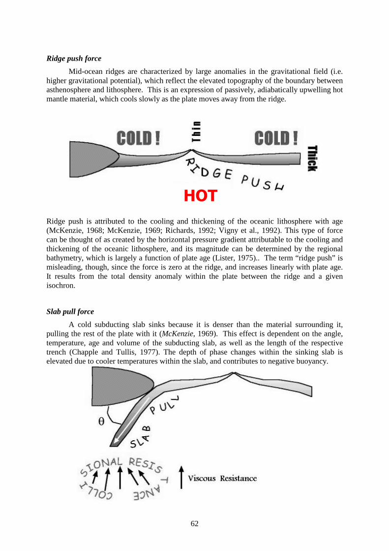
62

Ridge push force

Mid-ocean ridges are characterized by large anomalies in the gravitational field (i.e. higher gravitational potential), which reflect the elevated topography of the boundary between asthenosphere and lithosphere. This is an expression of passively, adiabatically upwelling hot mantle material, which cools slowly as the plate moves away from the ridge.

+27

Ridge push is attributed to the cooling and thickening of the oceanic lithosphere with age (McKenzie, 1968; McKenzie, 1969; Richards, 1992; Vigny et al., 1992). This type of force can be thought of as created by the horizontal pressure gradient attributable to the cooling and thickening of the oceanic lithosphere, and its magnitude can be determined by the regional bathymetry, which is largely a function of plate age (Lister, 1975).. The term “ridge push” is misleading, though, since the force is zero at the ridge, and increases linearly with plate age. It results from the total density anomaly within the plate between the ridge and a given isochron.

Slab pull force

A cold subducting slab sinks because it is denser than the material surrounding it, pulli ng the rest of the plate with it (McKenzie, 1969). This effect is dependent on the angle, temperature, age and volume of the subducting slab, as well as the length of the respective trench (Chapple and Tulli s, 1977). The depth of phase changes within the sinking slab is elevated due to cooler temperatures within the slab, and contributes to negative buoyancy.

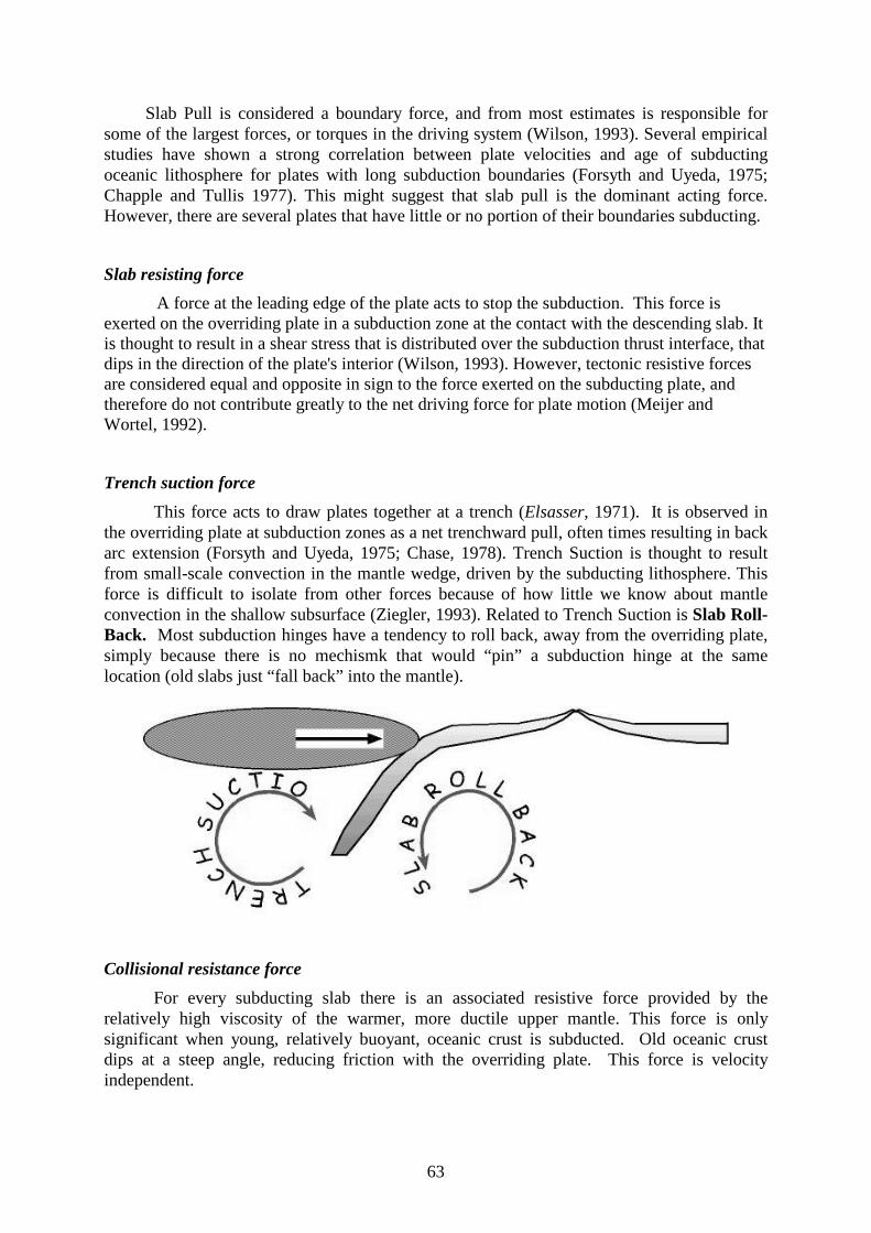
63

Slab Pull i s considered a boundary force, and from most estimates is responsible for

some of the largest forces, or torques in the driving system (Wilson, 1993). Several empirical studies have shown a strong correlation between plate velocities and age of subducting oceanic lithosphere for plates with long subduction boundaries (Forsyth and Uyeda, 1975; Chapple and Tulli s 1977). This might suggest that slab pull i s the dominant acting force. However, there are several plates that have littl e or no portion of their boundaries subducting.

Slab resisting force

A force at the leading edge of the plate acts to stop the subduction. This force is exerted on the overriding plate in a subduction zone at the contact with the descending slab. It is thought to result in a shear stress that is distributed over the subduction thrust interface, that dips in the direction of the plate's interior (Wilson, 1993). However, tectonic resistive forces are considered equal and opposite in sign to the force exerted on the subducting plate, and therefore do not contribute greatly to the net driving force for plate motion (Meijer and Wortel, 1992).

Trench suction force

This force acts to draw plates together at a trench (Elsasser, 1971). It is observed in the overriding plate at subduction zones as a net trenchward pull , often times resulting in back arc extension (Forsyth and Uyeda, 1975; Chase, 1978). Trench Suction is thought to result from small -scale convection in the mantle wedge, driven by the subducting lithosphere. This force is diff icult to isolate from other forces because of how littl e we know about mantle convection in the shallow subsurface (Ziegler, 1993). Related to Trench Suction is Slab Roll-Back. Most subduction hinges have a tendency to roll back, away from the overriding plate, simply because there is no mechismk that would “pin” a subduction hinge at the same location (old slabs just “ fall back” into the mantle).

Collisional resistance force

For every subducting slab there is an associated resistive force provided by the relatively high viscosity of the warmer, more ductile upper mantle. This force is only significant when young, relatively buoyant, oceanic crust is subducted. Old oceanic crust dips at a steep angle, reducing friction with the overriding plate. This force is velocity independent.

64

Together, the negative buoyancy of the sinking slab and the resistive nature of the slab entering the mantle is called the Net Slab Force. The sum of these two forces is exerted at the colliding margin (Ziegler, 1992) and contributes to the intra-plate stress field of the surface plates (Wilson, 1993).

Transform fault resistance force

The resistance at transform faults due to friction. The following diagrams are taken from Forsyth and Uyeda (1975), and show how the absolute motion velocities of plates correlate with their boundary characteristics and area.

Forces which drive plate motion: (1) Slab pull (2) Ridge push (3) Trench suction Forces which resist plate motion: (1) Slab resistance (2) Colliding resistance (3) Transform fault resistance The mantle drag forces are driving or resistive forces depending on the direction of

relative motion between the plate and underlying mantle.

65

Tectonic Stresses and Their Relationship to Plate Driving Forces

We will now look at information on the intraplate tectonic effects of plate motions, or in geologic terms, the associated stress related to these forces. In order to do this it is very important that we understand the regional patterns of the present-day tectonic stress field. Tectonic stresses are those stresses produced by the forces that drive plate tectonics (Middleton et al., 1996). Because of their integral relationship to the present motion of plates, the magnitude and direction of tectonic stress is very difficult to predict unless we can measure recent tectonic movement or seismic activity. In order to distinguish a measured tectonic stress from those stress fields that are locally derived, we must look at the spatial uniformity of the in situ stress field. For tectonic stresses the stress fields are typically uniform over distances many times (2 to more than 100 times) the thickness of the elastic part of the lithosphere, while local stresses are only a fraction of that same thickness (Zoback et al., 1989). It is also found that for tectonic fields the three principal stresses lie in approximately horizontal and vertical planes, with the horizontal stress component almost always larger than the vertical component. As a consequence the orientation of the principal stress axes of the measured stress tensor can be constrained by specifying the direction of just one of the horizontal principle stresses (Zoback, 1989). This is convenient for recording and measuring crustal stresses.

World Stress Map and topography/bathymetry

66

Once measured, tectonic stresses can give valuable information about the forces acting on the plates and therefore the dynamics of plate tectonics. A group of some 30 scientists from all over the world, headed by Mary Lou Zoback, have created a working database of in situ stress measurements for most of the Earth's lithospheric plates. They collected over 7300 in situ stress measurements, of which 4400 are considered tectonic stresses. These measurements were taken from bore-hole breakouts, hydraulic fractures, style of active faulting, volcanic alignment, seismic focal mechanisms, and transform fault azimuths. The entire database then underwent a scrutinous quality rating to asses the reliabilit y of the individual data, with any unsatisfactory data discarded (Zoback, 1989; Zoback, 1992).

The World Stress Map Project (WSMP), because of its huge database, has provided

significant advancement in our efforts to determine he relative importance of different plate driving forces. The project has also provided constraints on the magnitude of both broad scale and local stresses acting on the lithosphere. Subsequent analysis has shown that a majority of the data can be adequately explained by the geometry of plate boundaries and the conventional ridge push, slab pull , and subduction forces, and do not necessarily require a significant contribution from sublithospheric mantle flow inferred from seismic tomography (Zoback and Magee, 1991; Wilson, 1993). It appears that regionally uniform horizontal intra-plate stress orientations are consistent with either relative or absolute plate motions indicating that plate-boundary and body forces must be the dominant contributors to the stress distribution within plates (Zoback, 1989; Zoback, 1992).

Numerous observations suggest that drag forces and resisting forces do not strongly

control the stress field of the uppermost brittle part of the lithosphere. The general state of compression in the old oceanic lithosphere (older than ~80 Ma) indicates that the integrated ridge push force dominates over the associated mantle drag forces (Richards et al., 1992). Also, the predicted stresses related to whole mantle flow inferred from seismic tomography do not match well with the broadest scale tectonic stress data, especially when compared to the correlation of the boundary and body forces with tectonic directions (Zoback, 1992).

Correlations between the World Stress Map's tectonic stress measurements and PDF's

were immediately obvious after the measurements were plotted on a map of the Earth's plate boundaries. Normal faults that showed maximum tension perpendicular to ridge crests were seen for most of the world's spreading ridges. Old oceanic crust (>35 Ma) experiences mainly thrust or strike-slip faulting. This tectonic style is consistent with an intra-plate stress field dominated by compression associated with the net slab and/or ridge forces. Orientations of compressional stresses which dominate the interiors of most continental cratons, most importantly North America and Western Europe, are similar to those predicted for ridge push and slab forces (Zoback, 1992; Richards, 1992). Furthermore, stress measurements show, on a broad scale, stress fields changing in style (i.e. compressional to tensional) over individual plates with a tendency for the maximum horizontal stress direction (Sh Max) to be parallel to the absolute plate motion. This last fact is an important observation which directly relates to the relationship between plate boundary and body forces and the motion of plates. Using the evidence provided by the WSMP that plate boundary and body forces appear to dominate the driving mechanism of plate motion, the next step is to quantify the different magnitudes of the individual PDF's.

There are three different techniques geologists and geophysists have used in order to

quantify the different plate driving forces. Deformational modeling studies using intra-plate stress fields were popular in the late 1970's and early 1980's. Some of the earlier attempts

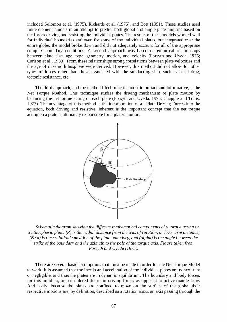
67

included Solomon et al. (1975), Richards et al. (1975), and Bott (1991). These studies used finite element models in an attempt to predict both global and single plate motions based on the forces driving and resisting the individual plates. The results of these models worked well for individual boundaries and even for some of the individual plates, but integrated over the entire globe, the model broke down and did not adequately account for all of the appropriate complex boundary conditions. A second approach was based on empirical relationships between plate size, age, type, geometry, motion, and velocity (Forsyth and Uyeda, 1975; Carlson et al., 1983). From these relationships strong correlations between plate velocities and the age of oceanic lithosphere were derived. However, this method did not allow for other types of forces other than those associated with the subducting slab, such as basal drag, tectonic resistance, etc.

The third approach, and the method I feel to be the most important and informative, is the

Net Torque Method. This technique studies the driving mechanism of plate motion by balancing the net torque acting on each plate (Forsyth and Uyeda, 1975; Chapple and Tulli s, 1977). The advantage of this method is the incorporation of all Plate Driving Forces into the equation, both driving and resistive. Inherent is the important concept that the net torque acting on a plate is ultimately responsible for a plate's motion.

Schematic diagram showing the different mathematical components of a torque acting on

a lithospheric plate. (R) is the radial distance from the axis of rotation, or lever arm distance, (Beta) is the co-latitude position of the plate boundary, and (alpha) is the angle between the

strike of the boundary and the azimuth to the pole of the torque axis. Figure taken from Forsyth and Uyeda (1975).

There are several basic assumptions that must be made in order for the Net Torque Model

to work. It is assumed that the inertia and acceleration of the individual plates are nonexistent or negligible, and thus the plates are in dynamic equili brium. The boundary and body forces, for this problem, are considered the main driving forces as opposed to active-mantle flow. And lastly, because the plates are confined to move on the surface of the globe, their respective motions are, by definition, described as a rotation about an axis passing through the

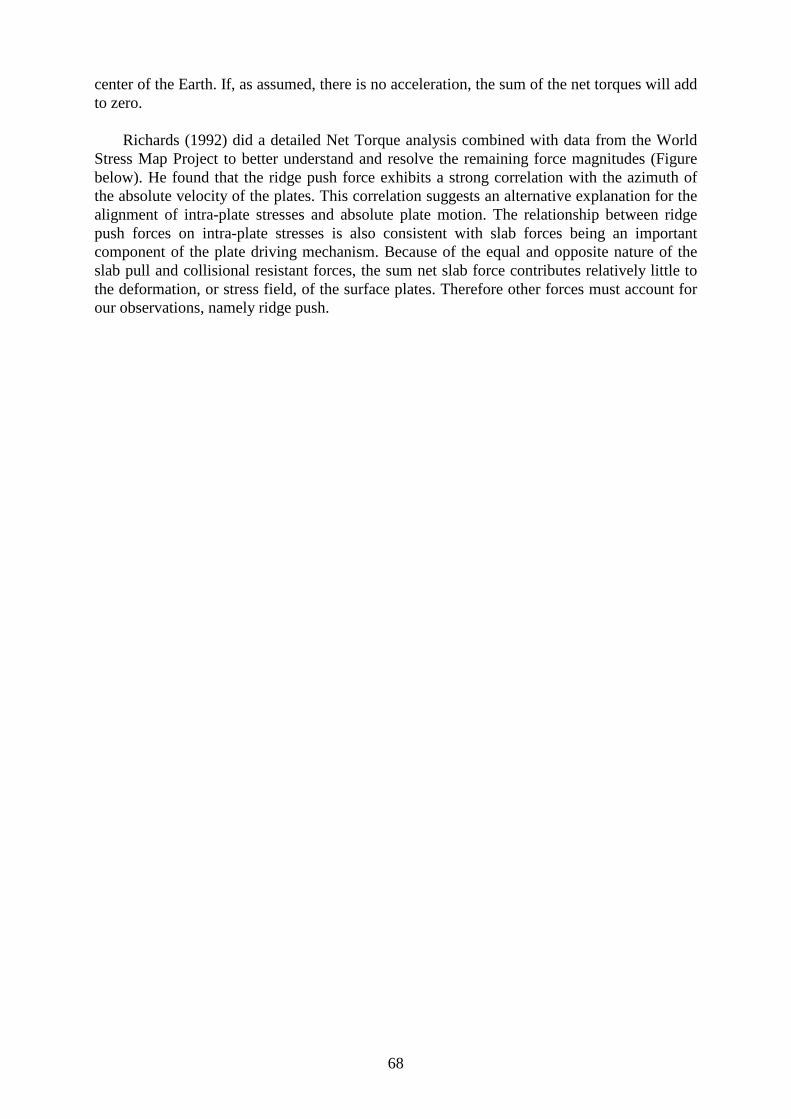
68

center of the Earth. If, as assumed, there is no acceleration, the sum of the net torques will add to zero.

Richards (1992) did a detailed Net Torque analysis combined with data from the World

Stress Map Project to better understand and resolve the remaining force magnitudes (Figure below). He found that the ridge push force exhibits a strong correlation with the azimuth of the absolute velocity of the plates. This correlation suggests an alternative explanation for the alignment of intra-plate stresses and absolute plate motion. The relationship between ridge push forces on intra-plate stresses is also consistent with slab forces being an important component of the plate driving mechanism. Because of the equal and opposite nature of the slab pull and collisional resistant forces, the sum net slab force contributes relatively little to the deformation, or stress field, of the surface plates. Therefore other forces must account for our observations, namely ridge push.

69

Ridge Boundaries and Force Directions in the top diagram, and Ridge Torque (black

arrows) vs. Absolute Velocity (gray arrows) in the lower diagram. Notice the nice correlation between the two vector directions (Richards, 1992)

To the question, "What drives plate tectonics?" we have two possible answers: (1) mantle

convection, and (2) lithospheric plate boundary and body forces. The above discussion points strongly to the plates themselves as being the dominant source of force involved in their absolute motion. The strong correlations between observed tectonic stress and absolute plate motions shown by the World Stress Map Project point directly to the present lithospheric stress fields being dominated by the individual plate boundary and body forces (Zoback et al., 1989, Zoback, 1992).

70

This solution for Plate Driving Forces works for today, but what about the past? Did slab and ridge forces always dominate, and did they always dominate in that order? These questions are important when considering the driving forces behind plate motion over time. Plates must rearrange themselves throughout supercontinent cycles, continuously changing the constructive and destructive nature of their boundaries. It is logical to assume then that these changes in the interactions and movements of plates must also change the relative importance of different plate driving forces in time and space. It follows then that the forces that drive plates are depenent on the nature of boundary conditions and plate arrangement through time.

There are still many unanswered questions related to plate driving forces. Can plate

driving forces be responsible for the breakup of supercontinents? Are plate boundary and/or plate body forces responsible for the initiation of subduction zones and spreading ridges? Most researchers believe in these special cases, mantle forces related to large convection cells must dominate the driving forces (Jacoby, 1980; Carlson et al, 1983;Wilson, 1991; Zeigler, 1991).

The Wilson Cycle Tuzo Wilson proposed that ocean basins experience a cyclical evolution, by opening, closing, followed by continental collision, and some time later opening once again. Many strands of evidence support this idea.

1) Formation of rift

Plates tend to aggregate over cold downwellings in the mantle, acting as an insulating blanket. The mantle underneath the plates heats up, alters the convection pattern, and the continent splits in response to intraplate-tension. Breakup of the continents produces rift valleys.

2) Extension and formation of rift valleys

The valley is filled with marine water and, eventually, oceanic crust is created. At the beginning of this stage mafic dikes form parallel to the edges of the emerging ocean.

The fault-bounded grabens are covered with shallow marine deposits. Drainage, largely away from the rift, limits the amount of clastic sedimentation. Restricted communication with open ocean water induces deposition of sabkha carbonates and evaporites. Accumulation of reef limestones is facilitated by the slow subsidence rates and lack of terrigenous sediments. Anaerobic conditions may develop near the bottom and produce sapropelic carbonaceous mud.

71

Existence of possible source rocks (i.e. sapropelic mud) as well as reservoir rocks (i. e. reef limestones) and potential structural traps (evaporites-salt domes) provides favorable conditions for the hydrocarbon accumulation in this setting. Ore deposits include stratiform copper deposits and lead-zinc-barite ores.

3) Young ocean basin

New oceanic crust is continuously generated at the mid oceanic ridge. The rise divides the ocean in two halves with separate depositional histories. In the early stage certain amount of symmetry exists between the two margins due to the relatively small distance.

A basic terrigenous clastic wedge formed at the periphery of the continental shelf reflects the rapid thermotectonic subsidence. Accelerated spreading in this stage leads to the global transgression with a possible change in climate and biological activity. The amount of oxygen in the seawater may be reduced, inducing formation of sapropelic muds. Terrigenous clastic wedge grades laterally into the fluvio lacustrine complex and seaward in to turbidites of the continental rise. Calcareous sediments are deposited in the central parts of the ocean on the flanks of the ridge that lie above the carbonate compensation depth (CCD). Red clays are deposited bellow the CCD.

72

Ore deposits in this setting are related to midoceanic ridges and to the growing areas of open ocean. Burial of sapropelic deposits by the clastic sediments of the continental margins may create favorable conditions for the formation of hydrocarbons.

4) Mature ocean basin

Due to the continuous production of oceanic crust at the midoceanic ridge, the basin has achieved considerable width. Two distant continental margins are unrelated and asymmetrical.

On the passive edges large amounts of sediments are accumulated. Flexural subsidence dominates. Compared to the previous stage, subsidence rates are much slower permitting formation of carbonate platforms (Great Bahama Bank). On the basal clastic wedge, deltaic, lacustrine and shelf deposits accumulate, building the continental terrace and embankment. Turbidite currents transport sediments down the continental slope to the continental rise. In the open ocean, red clays accumulate below, and calcareous oozes above the carbonate compensation depth. In addition to the mineralization at the midoceanic ridge, on the oceanic bottom, ferro manganese nodules and encrustrations are formed. These hydrous sediments accumulate slowly and may form extensive pavements. Passive continental margins have a high potential for the formation of hydrocarbons. Possible source rocks include: prodelta shales, shaley turbidite deposits, carbonates and shales of continental shelf and phosphorites. Maturation of the hydrocarbons is facilitated by the great thickness of overlaying sediments. Deltaic sediments, sediments of carbonate shelves and turbidites are possible reservoir rocks. Structural and depositional characteristics of passive margins provide conditions for the formation of effective hydrocarbon traps (salt diapires, faults). The south, east, and west coasts of Australia are modern examples.

5) Closing of the Ocean

Production of the oceanic crust at midoceanic ridges is compensated by the subduction of oceanic crust on convergent plate boundaries.

73

Ocean-island arc collision

Continent-ocean collision

The structure of the accretionary wedge is characterized by a series of imbricated listric faults dipping toward the arc. Melange, a mass of chaotically mixed brecciated blocks in a highly sheared matrix, is a characteristic type of sediment. Scrapings from the subducted plate usually include terrigenous and pelagic sedimentary blocks and oceanic ophiolites. Blueschist grade metamorphism, characterized with high pressure and relatively low temperature, is typical for this setting. Gold-rich porphyry copper deposits and stratiform massive sulphides of zinc, lead and copper, (Kuroko-type) ores are associated with island arcs. Marginal seas and forearc basins have potential for the formation and preservation of hydrocarbons.

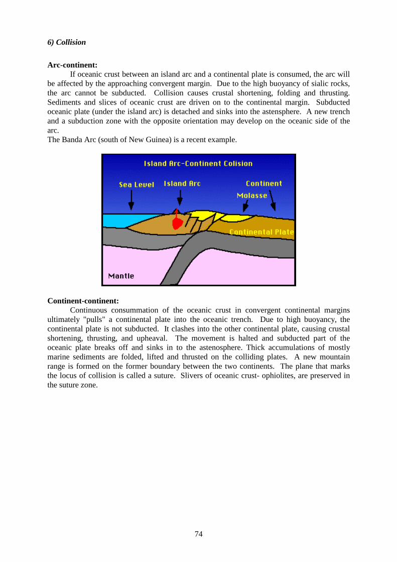
74

6) Collision

Arc-continent: If oceanic crust between an island arc and a continental plate is consumed, the arc will be affected by the approaching convergent margin. Due to the high buoyancy of sialic rocks, the arc cannot be subducted. Collision causes crustal shortening, folding and thrusting. Sediments and slices of oceanic crust are driven on to the continental margin. Subducted oceanic plate (under the island arc) is detached and sinks into the astensphere. A new trench and a subduction zone with the opposite orientation may develop on the oceanic side of the arc. The Banda Arc (south of New Guinea) is a recent example.

Continent-continent: Continuous consummation of the oceanic crust in convergent continental margins ultimately "pulls" a continental plate into the oceanic trench. Due to high buoyancy, the continental plate is not subducted. It clashes into the other continental plate, causing crustal shortening, thrusting, and upheaval. The movement is halted and subducted part of the oceanic plate breaks off and sinks in to the astenosphere. Thick accumulations of mostly marine sediments are folded, lifted and thrusted on the colliding plates. A new mountain range is formed on the former boundary between the two continents. The plane that marks the locus of collision is called a suture. Slivers of oceanic crust- ophiolites, are preserved in the suture zone.

75

Volcanic rocks formed include: andesite, dacite, rhyolite and alkali basalts. Extensive plutons form consisting of granite, quartz monzonite etc. In the Himalayan type of orogenic belts, three zones can be distinguished on the basis of morphology: foreland basin, thrust belt, and plateau. Typical sediments for this setting are molasse and flysch. Formation of f lysch is related to the early stages of mountain building. Flysch sediments are synorogenetic. They consist of marine shaly formations with the intercalations of sandstone and impure limestone. Molasse sediments occur in the final stage of mountain building, typically in the foreland basin. They are late to postorogentic deposits consisting of f luvial and lacustrine sandstones, red beds and shales. During deposition of molasse sediments, conditions can fluctuate between the nonmarine and marine. Sequences with lignite, coal, freshwater limestones and evaporites may occur. The Himalaya mountains are a modern example. Mineralization: Deposits typical for earlier stages of Wilson's cyclus can occur in the alochtonous members within the colli sional environment. Tungsten, cassiterite, and wolframite deposits are related to the granites that are implaced during the orogeny. Hydrocarbons occur in the foreland basins of the Himalyan-type mountain ranges (e.g.Aquitane Basin, SW France).

7) Renewed breakup

Eventually, a new rift and ocean basin may form along an old suture. Example: Paleozoic Iapetus ocean between Eurasia and North America was followed by colli sion (formation of Apallachians), and subsequent opening of Atlantic ocean along old suture.

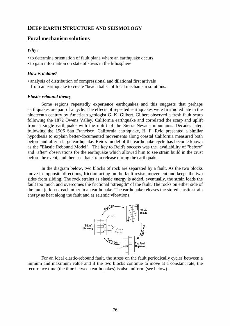
76

DEEP EARTH STRUCTURE AND SEISMOLOGY

Focal mechanism solutions

Why?

• to determine orientation of fault plane where an earthquake occurs • to gain information on state of stress in the lithosphere

How is it done?

• analysis of distribution of compressional and dilational first arrivals from an earthquake to create "beach balls" of focal mechanism solutions.

Elastic rebound theory

Some regions repeatedly experience earthquakes and this suggests that perhaps earthquakes are part of a cycle. The effects of repeated earthquakes were first noted late in the nineteenth century by American geologist G. K. Gilbert. Gilbert observed a fresh fault scarp following the 1872 Owens Valley, Cali fornia earthquake and correlated the scarp and upli ft from a single earthquake with the upli ft of the Sierra Nevada mountains. Decades later, following the 1906 San Francisco, Cali fornia earthquake, H. F. Reid presented a similar hypothesis to explain better-documented movements along coastal Cali fornia measured both before and after a large earthquake. Reid's model of the earthquake cycle has become known as the "Elastic Rebound Model". The key to Reid's success was the availabilit y of "before" and "after" observations for the earthquake which allowed him to see strain build in the crust before the event, and then see that strain release during the earthquake.

In the diagram below, two blocks of rock are separated by a fault. As the two blocks move in opposite directions, friction acting on the fault resists movement and keeps the two sides from sliding. The rock strains as elastic energy is added, eventually, the strain loads the fault too much and overcomes the frictional "strength" of the fault. The rocks on either side of the fault jerk past each other in an earthquake. The earthquake releases the stored elastic strain energy as heat along the fault and as seismic vibrations.

For an ideal elastic-rebound fault, the stress on the fault periodically cycles between a

inimum and maximum value and if the two blocks continue to move at a constant rate, the recurrence time (the time between earthquakes) is also uniform (see below).

77

Dislocation model for an earthquake

Realistic fault structure

Simplified dislocation model

Side view into the earth's crust showing rupture of the rocks spreading out from the focus of the earthquake along the dipping fault plane. Black arrows show spreading of the dislocation, the area of rupture, hollow arrows show the direction of slip as viewed from this

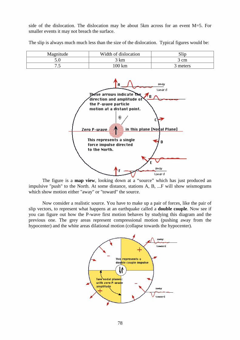
78

side of the dislocation. The dislocation may be about 5km across for an event M=5. For smaller events it may not breach the surface. The slip is always much much less than the size of the dislocation. Typical figures would be:

Magnitude Width of dislocation Slip 5.0 3 km 3 cm 7.5 100 km 3 meters

The figure is a map view, looking down at a “source” which has just produced an impulsive "push" to the North. At some distance, stations A, B, ...F will show seismograms which show motion either "away" or "toward" the source. Now consider a realistic source. You have to make up a pair of forces, li ke the pair of slip vectors, to represent what happens at an earthquake called a double couple. Now see if you can figure out how the P-wave first motion behaves by studying this diagram and the previous one. The grey areas represent compressional motion (pushing away from the hypocenter) and the white areas dilational motion (collapse towards the hypocenter).

79

The common approach to focal mechanism studies of shallow earthquakes is to use the first motion of the primary or P-wave, the first seismic wave to arrive. A seismograph detects a push (compression) or pull (dilatation) that indicates the direction of ground movement at that point. Seismologists trace first-motion data from various seismographs backward to the focal sphere, an imaginary sphere surrounding the focus. Because these data are diff icult to plot on a sphere and interpret, they are projected onto a plane that bisects the sphere, as seen in the following figure for different types of faulting.

Note that the fault plane here is E-W oriented, coinciding with one of the dividing lines on our “beach ball ” slice. Seismologists commonly differentiate types of motion by dark (compressional) and light (dilatational) zones, resulting in a "beach ball ." The two lines

80

separating the quadrants represent perpendicular planes, called nodal planes, that depict areas without P-wave motion. These are the fault and auxiliary planes. If we had no independent, geological information on whether the fault actually runs E-W or N-S, we would not be able to tell from the pattern of compression and dilation alone which plane corresponds to the fault plane.

Consider an earthquake that formed along a strike-slip fault as shown above. We have constructed an “ imaginary” sphere around the hypocenter, and removed the upper half of it. Now, we project all first p-wave motions (compressional or dilational) from different points on the lower half of the sphere onto the equatorial plane. As a result, we obtain the disk

81

shown above and below the focal hemipshere, whose dark and light areas represent compressional and dilational first motions, respectively. Projections, or fault plane solutions, are by convention always from the lower (southern) focal hemisphere. Each is simply a flat representation of the lower half of the focal sphere as viewed from directly above the focus (at the epicenter),

A plane: a) passing through a sphere; b) within sphere; c) within lower hemisphere; d) within lower hemisphere, viewed from above. The equatorial plane is green in each of the diagrams in this figure. Below the zones of compressional (P-wave up) and dilatational (P-wave down) first motion from an earthquake on a right lateral strike slip fault are shown on a model earth.

The zones of compression and dilatation for a right lateral, strike slip fault are shown on a spherical model earth. A P-wave recorded by a seismograph in a dark area will have an up (compressional) first motion while a P-wave recorded in a light area will have a down (dilatational) first motion. The plan view is a close-up of the epicentral area.

82

In the fault plane solution of a vertical strike-slip fault the nodal planes are shown as perpendicular lines that intersect at the center of the projection. This provides two possible solutions for the fault plane: 1) a right lateral fault trending northwest and 2) a left lateral trending northeast. Geological information, such as rupture of the Earth's surface, is needed to determine which of the two nodal planes is the fault plane and which is the auxili ary.

Fault plane solution for a vertical strike-slip fault. The arrows have been added to indicate direction of movement (right lateral). Note the arrows move toward the areas of compression on each side of the fault. If the motion on a vertical fault is oblique, that is, it includes components of strike slip and dip slip, the auxili ary plane will plot as a line curving toward the circumference (Figure 4).

Fault plane solution for a vertical oblique-slip (part strike slip and part dip slip) fault. The strike slip component is right lateral. The auxili ary plane wil l intersect the line representing the fault plane between the circle and its center. The closer the intersection is to the center, the more dominant the strike slip. For pure dip slip on a vertical fault the auxili ary plane is the equatorial plane (Figure 5).

83

Fault plane solution for a vertical dip-slip fault.

The line representing a vertical fault passes through the center of the circle (Figures 4 and 5) but those depicting normal or reverse faults are curved and meet at the circumference (Figures 6 and 7). The greater the curve is (the closer to the circumference), the shallower the dip. The strike of a nodal plane is measured in degrees around the circle from north to the line of the nodal plane (Figure 8).

Fault plane solution for an east-dipping normal fault.

84

Fault plane solution for an east-dipping reverse fault.

Focal plane solutions: a) normal fault striking north, dipping east or west approximately 45 degrees; b) oblique fault, right lateral and reverse slip (attitude approximately N50E/20W) or left lateral and reverse slip (attitude approximately N5W/80E); c) oblique fault, reverse slip dominant, with some right lateral (attitude approximately N35W/50W) or left lateral (attitude approximately N55W/40E); d) oblique fault, strike slip dominant, attitude approximately N40W/70W (right lateral), or N35E/70E (left lateral).

85

DEEP EARTH STRUCTURE INTRODUCTION Five billi on years ago the Earth was formed in a massive conglomeration and bombardment of meteorites and comets. The immense amount of heat energy released by the high-velocity bombardment melted the entire planet, and it is still cooling off today. Denser materials li ke iron (Fe) from the meteroites sank into the core of the Earth, while lighter sili cates (Si), other oxygen (O) compounds, and water from comets rose near the surface. The Earth is divided into four main layers: the inner core, outer core, mantle, and crust. The core is composed mostly of iron (Fe) and is so hot that the outer core is molten, with about 10% sulphur (S). The inner core is under such extreme pressure that it remains solid. Most of the Earth's mass is in the mantle, which is composed of iron (Fe), magnesium (Mg), aluminum (Al), sili con (Si), and oxygen (O) sili cate compounds. At over 1000 degrees C, the mantle is solid but can deform slowly in a plastic manner. The crust is much thinner than any of the other layers, and is composed of the least dense calcium (Ca) and sodium (Na) aluminum-sili cate minerals. Being relatively cold, the crust is rocky and brittle, so it can fracture in earthquakes.

EARTHQUAKE SEISMOLOGY

Introduction Earthquake seismology provides the main tool to gather information about the deep

structure of the Earth. An earthquake is the vibration of the Earth's surface that follows a release of energy in the Earth's crust. This energy can be generated by a sudden dislocation of segments of the crust, by a volcanic eruption, or event by manmade explosions. Most destructive quakes, however, are caused by dislocations of the crust.

The crust may first bend and then, when the stress exceeds the strength of the rocks,

break and "snap" to a new position. In the process of breaking, vibrations called "seismic waves" are generated. These waves travel outward from the source of the earthquake along the surface and through the Earth at varying speeds depending on the material through which they move. Some of the vibrations are of high enough frequency to be audible, while others are of very low frequency.

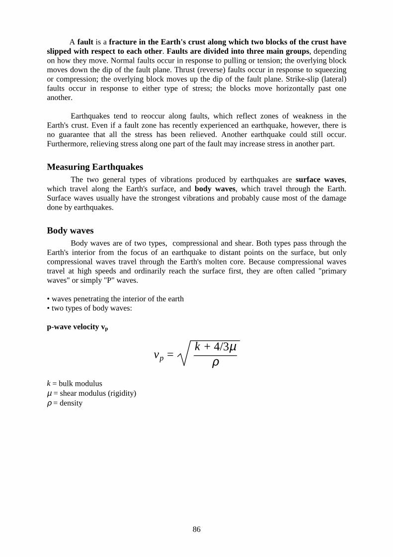
86

A fault is a fracture in the Earth's crust along which two blocks of the crust have slipped with respect to each other. Faults are divided into three main groups, depending on how they move. Normal faults occur in response to pulli ng or tension; the overlying block moves down the dip of the fault plane. Thrust (reverse) faults occur in response to squeezing or compression; the overlying block moves up the dip of the fault plane. Strike-slip (lateral) faults occur in response to either type of stress; the blocks move horizontally past one another.

Earthquakes tend to reoccur along faults, which reflect zones of weakness in the Earth's crust. Even if a fault zone has recently experienced an earthquake, however, there is no guarantee that all the stress has been relieved. Another earthquake could still occur. Furthermore, relieving stress along one part of the fault may increase stress in another part.

Measur ing Ear thquakes The two general types of vibrations produced by earthquakes are sur face waves,

which travel along the Earth's surface, and body waves, which travel through the Earth. Surface waves usually have the strongest vibrations and probably cause most of the damage done by earthquakes.

Body waves Body waves are of two types, compressional and shear. Both types pass through the

Earth's interior from the focus of an earthquake to distant points on the surface, but only compressional waves travel through the Earth's molten core. Because compressional waves travel at high speeds and ordinarily reach the surface first, they are often called "primary waves" or simply "P" waves. • waves penetrating the interior of the earth • two types of body waves: p-wave velocity vp

vp = k + 4/3µ

ρ

k = bulk modulus µ = shear modulus (rigidity) ρ = density

87

Shear waves do not travel as rapidly through the Earth's crust and mantle as do

compressional waves, and because they ordinarily reach the surface later, they are called "secondary" or "S" waves. Instead of affecting material directly behind or ahead of their line of travel, shear waves displace material at right angles to their path and therefore sometimes called "transverse" waves.

s-wave velocity vs:

vs = µρ vp ~ vs * 1.7

• rigidity of f luids is zero –> fluids cannot transmit S-waves

Surface waves • surface waves are restricted to the vicinity of a free surface • 2 types of surface waves: • Rayleigh waves: particles move in elli pse in a vertical plane • Love waves: are transmitted whenever the S-wave velocity of the surface layer is lower

than that of the underlying layer. • horizontally polarized shear waves propagate by multiple reflections within this low-

velocity layer, which acts as wave guide • velocities of surface waves are lower than body wave velocities

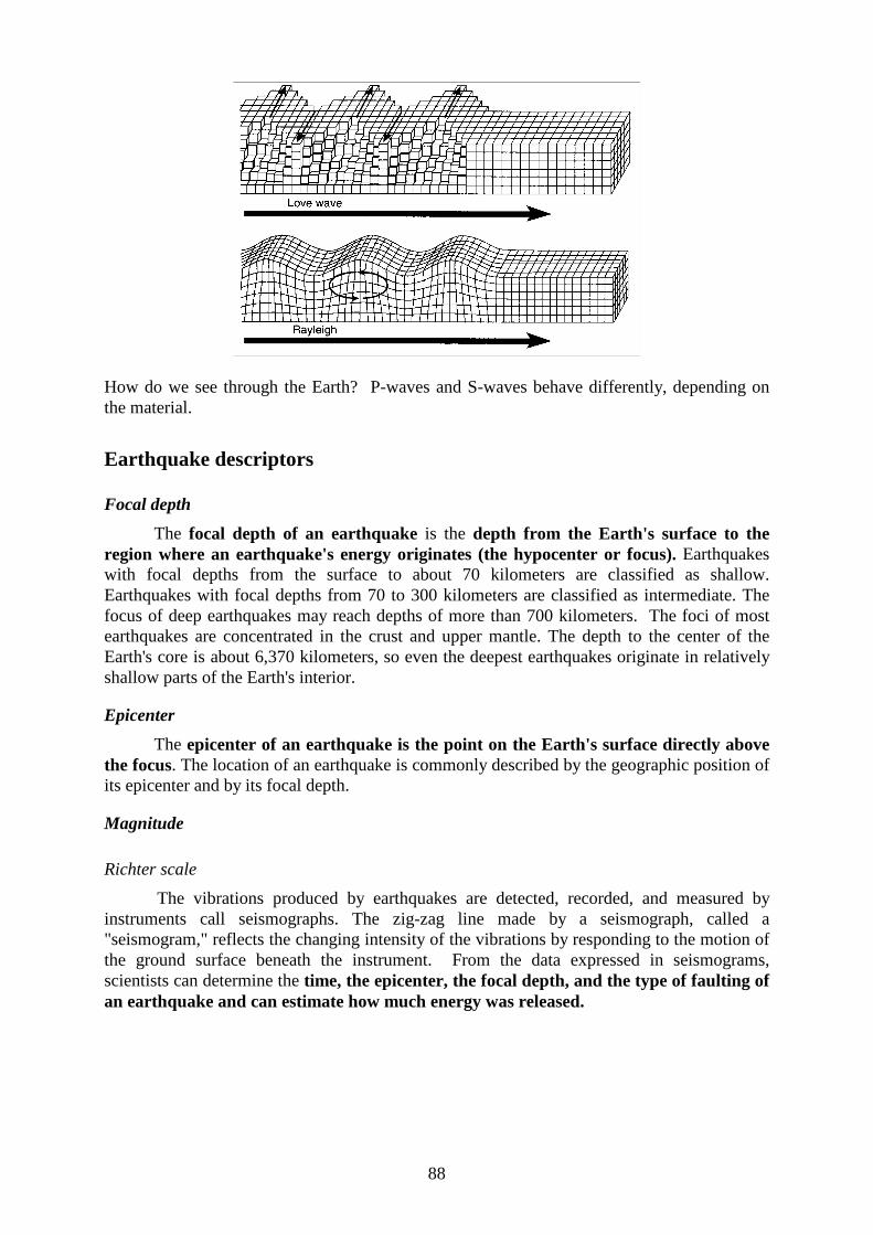
88

How do we see through the Earth? P-waves and S-waves behave differently, depending on the material.

Earthquake descriptors

Focal depth

The focal depth of an ear thquake is the depth from the Earth's sur face to the region where an ear thquake's energy or iginates (the hypocenter or focus). Earthquakes with focal depths from the surface to about 70 kilometers are classified as shallow. Earthquakes with focal depths from 70 to 300 kilometers are classified as intermediate. The focus of deep earthquakes may reach depths of more than 700 kilometers. The foci of most earthquakes are concentrated in the crust and upper mantle. The depth to the center of the Earth's core is about 6,370 kilometers, so even the deepest earthquakes originate in relatively shallow parts of the Earth's interior.

Epicenter

The epicenter of an ear thquake is the point on the Earth's sur face directly above the focus. The location of an earthquake is commonly described by the geographic position of its epicenter and by its focal depth.

Magnitude

Richter scale

The vibrations produced by earthquakes are detected, recorded, and measured by instruments call seismographs. The zig-zag line made by a seismograph, called a "seismogram," reflects the changing intensity of the vibrations by responding to the motion of the ground surface beneath the instrument. From the data expressed in seismograms, scientists can determine the time, the epicenter, the focal depth, and the type of faulting of an ear thquake and can estimate how much energy was released.

89

Relationship between distance, travel time, earthquake magnitude and amplitude of ground

motion The magnitude of an earthquake describes its energy release on a logarithmic scale. The Richter Scale, named after Dr. Charles F. Richter of the Cali fornia Institute of Technology, is the best known scale for measuring the magnitude of earthquakes and was introduced in the 1930's, based on earthquakes in Cali fornia only. Basically, this scale measures the maximum signal amplitude recorded on a standard seismograph, which is then corrected for distance and instrument gain to obtain the magnitude. To find the magnitude, one measures the maximum amplitude A from a photographic record of a seismometer using a metric ruler. The formula for determining the Richter magnitude is

ML=log10(A) - log10(A0) where A0 is the distance/gain correction term, calibrated so that an earthquake 100 kilometers distant with a maximum amplitude of 1 millimeter would be assigned magnitude 3.

Surface wave magnitude

The Richter scale concept evolved to include world-wide earthquakes of any distance and depth, and later evolved further into two scales used in global earthquake catalogs: the MS (surface wave) and mb (body wave) scales. For most shallow earthquakes, surface waves, or waves that propagate along the surface of the Earth, are the greatest amplitude waves recorded on a seismogram. Therefore, a scale based on the amplitude of the surface wave is natural and convenient. After measuring the maximum surface wave amplitude A, the surface wave magnitude is given by

MS=log10(A/T)+1.66log10(D)+3.30 where T is the measured wave period and D is the distance in radians.

90

Body wave magnitude

Earthquakes occurring deep in the Earth do not generate large surface waves. Therefore, we also need a scale based on body waves, the seismic waves that travel through the Earth's interior or body. To determine body wave magnitude, we measure the maximum amplitude A and then calculate

mb=log10(A/T)+Q(D,h) where T is the measured wave period and Q is an empirical function of focal depth h and epicentral distance D. Currently the mb scale uses compressional body waves with a period of about 1 second, and the MS scale uses Rayleigh surface waves with 18 to 22 second periods. In general, all these scales may yield different magnitudes for any particular earthquake as well as negative magnitudes for very small earthquakes.

Why so many magnitude scales?

Each magnitude scale was initially designed for a particular class of seismograph, and for specific types of seismic waves. For example, surface waves create the strongest disturbance only within the upper layers of the Earth, perhaps to a few hundred kilometers depth. Shallow earthquakes excite especially large surface waves whereas deep earthquakes do not generate nearly as much surface wave energy. Therefore, MS generally underestimates the size of deep earthquakes. In constrast, body waves are well developed for both shallow and deep earthquakes, so mb can be used to compare them. However, body waves are more diff icult to observed than suface waves due to interactions with the interior structure of the Earth. While magnitude is a useful, simple, and widely understood concept, problems exist with assigning and interpreting magnitudes. Since seismologists define magnitude in terms of the response of a specific instrument at a specific distance and period, magnitude contains littl e information about the physics of the earthquake source. Moreover, earthquakes radiate energy unequally in all directions. For example, a magnitude estimated using a seismograph located directly North of an earthquake may not be the same as a magnitude estimated using a seismograph located directly East of an earthquake. For all these reasons, small differences in magnitudes have littl e physical significance. Lastly, the magnitude scales do not fully measure the size of large earthquakes because they are not sensitive to all of the earthquake waves. This scale "saturation" occurs around magnitude 8 for the MS scale, and around magnitude 6.5 for the mb scale. In contrast, moment magnitude (MW) does not saturate at large magnitudes and relies on an underlying robust physical and mathematical development. To find moment magnitude, one simply converts seismic moment using an algebraic formula calibrated to agree with MS over much of its range.

What is earthquake moment?

Earthquake moment, or seismic moment M0 is perhaps the most fundamental parameter we can use to measure the strength of an earthquake. While magnitudes are a convenient measure of earthquake size determined directly from one seismogram, M0 is a more physically meaningful measurement of earthquake size not subject to many of the problems that plague magnitudes. In fact, M0 is directly related to the fundamental parameters of the faulting process. Seismologists write this relationship as

91

where the greek letter mu is a constant called rigidity, A is the ruptured area of the fault, and s-bar is the average displacement over the fault. Seismic moment M0 usually has the units of dyne-centimeters or Newton-meters. Generally, finding M0 requires using all three components of data from all available seismic stations, encompassing many different distances and azimuths from the earthquake.

P- and S-wave paths through the Earth originating from the 1995 Kobe earthquake

The Preliminary Reference Earth Model (PREM) from Anderson (1989)

92

Vp = P-wave velocity Vs = S-wave velocity ρ = density Compressional P waves will t ravel and refract through both fluid and solid materials. Shear S waves, however, cannot travel through fluids like air or water. Fluids cannot support the side-to-side particle motion that makes S waves.

Seismologists noticed that records from an earthquake made around the world changed radically once the event was more than a certain distance away, about 105 degrees in terms of the angle between the earthquake and the seismograph at the center of the earth. After 105 degrees the waves disappeared almost completely, at least until the slow surface waves would arrive from over the horizon. The area beyond 105 degrees distance forms a shadow zone. At larger distances, some P waves would arrive, but still no S waves. Conclusion: The Earth has to have a molten, fluid core to explain the lack of S waves in the shadow zone, and the bending of P waves. You can get a rough estimate of the size of the Earth's core by simply assuming that the last S wave, before the shadow zone starts at 105 degrees, travels in a straight line. Knowing that the Earth has a radius of about 6350 km, you have a right triangle where the cosine of half of 105 degrees equals the radius of the core divided by the radius of the earth.

Estimation of the size of the Earth's core

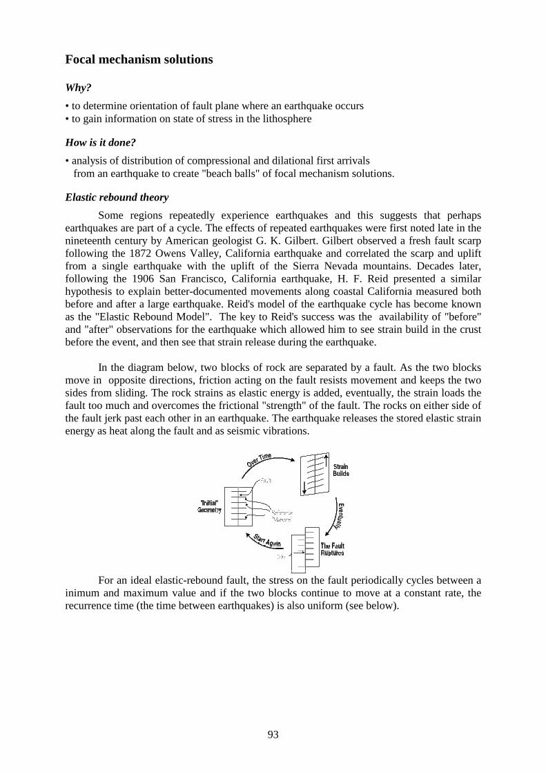
93

Focal mechanism solutions

Why?

• to determine orientation of fault plane where an earthquake occurs • to gain information on state of stress in the lithosphere

How is it done?

• analysis of distribution of compressional and dilational first arrivals from an earthquake to create "beach balls" of focal mechanism solutions.

Elastic rebound theory

Some regions repeatedly experience earthquakes and this suggests that perhaps earthquakes are part of a cycle. The effects of repeated earthquakes were first noted late in the nineteenth century by American geologist G. K. Gilbert. Gilbert observed a fresh fault scarp following the 1872 Owens Valley, Cali fornia earthquake and correlated the scarp and upli ft from a single earthquake with the upli ft of the Sierra Nevada mountains. Decades later, following the 1906 San Francisco, Cali fornia earthquake, H. F. Reid presented a similar hypothesis to explain better-documented movements along coastal Cali fornia measured both before and after a large earthquake. Reid's model of the earthquake cycle has become known as the "Elastic Rebound Model". The key to Reid's success was the availabilit y of "before" and "after" observations for the earthquake which allowed him to see strain build in the crust before the event, and then see that strain release during the earthquake.

In the diagram below, two blocks of rock are separated by a fault. As the two blocks move in opposite directions, friction acting on the fault resists movement and keeps the two sides from sliding. The rock strains as elastic energy is added, eventually, the strain loads the fault too much and overcomes the frictional "strength" of the fault. The rocks on either side of the fault jerk past each other in an earthquake. The earthquake releases the stored elastic strain energy as heat along the fault and as seismic vibrations.

For an ideal elastic-rebound fault, the stress on the fault periodically cycles between a

inimum and maximum value and if the two blocks continue to move at a constant rate, the recurrence time (the time between earthquakes) is also uniform (see below).

94

Dislocation model for an earthquake

Realistic fault structure

Simplified dislocation model

Side view into the earth's crust showing rupture of the rocks spreading out from the focus of the earthquake along the dipping fault plane. Black arrows show spreading of the dislocation, the area of rupture, hollow arrows show the direction of slip as viewed from this

95

side of the dislocation. The dislocation may be about 5km across for an event M=5. For smaller events it may not breach the surface. The slip is always much much less than the size of the dislocation. Typical figures would be:

Magnitude Width of dislocation Slip 5.0 3 km 3 cm 7.5 100 km 3 meters

The figure is a map view, looking down at a “source” which has just produced an impulsive "push" to the North. At some distance, stations A, B, ...F will show seismograms which show motion either "away" or "toward" the source. Now consider a realistic source. You have to make up a pair of forces, li ke the pair of slip vectors, to represent what happens at an earthquake called a double couple. Now see if you can figure out how the P-wave first motion behaves by studying this diagram and the previous one. The grey areas represent compressional motion (pushing away from the hypocenter) and the white areas dilational motion (collapse towards the hypocenter).

96

The common approach to focal mechanism studies of shallow earthquakes is to use the first motion of the primary or P-wave, the first seismic wave to arrive. A seismograph detects a push (compression) or pull (dilatation) that indicates the direction of ground movement at that point. Seismologists trace first-motion data from various seismographs backward to the focal sphere, an imaginary sphere surrounding the focus. Because these data are diff icult to plot on a sphere and interpret, they are projected onto a plane that bisects the sphere, as seen in the following figure for different types of faulting.

Note that the fault plane here is E-W oriented, coinciding with one of the dividing lines on our “beach ball ” slice. Seismologists commonly differentiate types of motion by dark (compressional) and light (dilatational) zones, resulting in a "beach ball ." The two lines

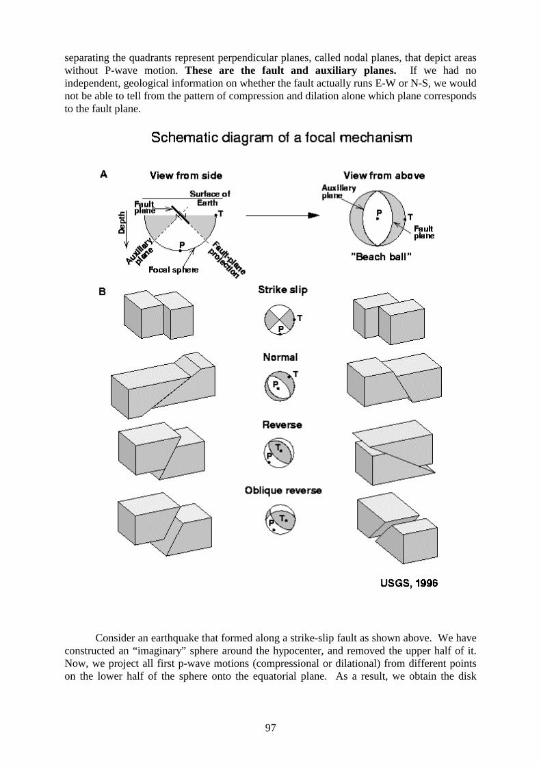
97

separating the quadrants represent perpendicular planes, called nodal planes, that depict areas without P-wave motion. These are the fault and auxiliary planes. If we had no independent, geological information on whether the fault actually runs E-W or N-S, we would not be able to tell from the pattern of compression and dilation alone which plane corresponds to the fault plane.

Consider an earthquake that formed along a strike-slip fault as shown above. We have constructed an “ imaginary” sphere around the hypocenter, and removed the upper half of it. Now, we project all first p-wave motions (compressional or dilational) from different points on the lower half of the sphere onto the equatorial plane. As a result, we obtain the disk

98

shown above and below the focal hemipshere, whose dark and light areas represent compressional and dilational first motions, respectively. Projections, or fault plane solutions, are by convention always from the lower (southern) focal hemisphere. Each is simply a flat representation of the lower half of the focal sphere as viewed from directly above the focus (at the epicenter),

A plane: a) passing through a sphere; b) within sphere; c) within lower hemisphere; d) within lower hemisphere, viewed from above. The equatorial plane is green in each of the diagrams in this figure. Below the zones of compressional (P-wave up) and dilatational (P-wave down) first motion from an earthquake on a right lateral strike slip fault are shown on a model earth.

The zones of compression and dilatation for a right lateral, strike slip fault are shown on a spherical model earth. A P-wave recorded by a seismograph in a dark area will have an up (compressional) first motion while a P-wave recorded in a light area will have a down (dilatational) first motion. The plan view is a close-up of the epicentral area.

99

In the fault plane solution of a vertical strike-slip fault the nodal planes are shown as perpendicular lines that intersect at the center of the projection. This provides two possible solutions for the fault plane: 1) a right lateral fault trending northwest and 2) a left lateral trending northeast. Geological information, such as rupture of the Earth's surface, is needed to determine which of the two nodal planes is the fault plane and which is the auxili ary.

Fault plane solution for a vertical strike-slip fault. The arrows have been added to indicate direction of movement (right lateral). Note the arrows move toward the areas of compression on each side of the fault. If the motion on a vertical fault is oblique, that is, it includes components of strike slip and dip slip, the auxili ary plane will plot as a line curving toward the circumference (Figure 4).

Fault plane solution for a vertical oblique-slip (part strike slip and part dip slip) fault. The strike slip component is right lateral. The auxili ary plane will i ntersect the line representing the fault plane between the circle and its center. The closer the intersection is to the center, the more dominant the strike slip. For pure dip slip on a vertical fault the auxili ary plane is the equatorial plane (Figure 5).

100

Fault plane solution for a vertical dip-slip fault.

The line representing a vertical fault passes through the center of the circle (Figures 4 and 5) but those depicting normal or reverse faults are curved and meet at the circumference (Figures 6 and 7). The greater the curve is (the closer to the circumference), the shallower the dip. The strike of a nodal plane is measured in degrees around the circle from north to the line of the nodal plane (Figure 8).

Fault plane solution for an east-dipping normal fault.

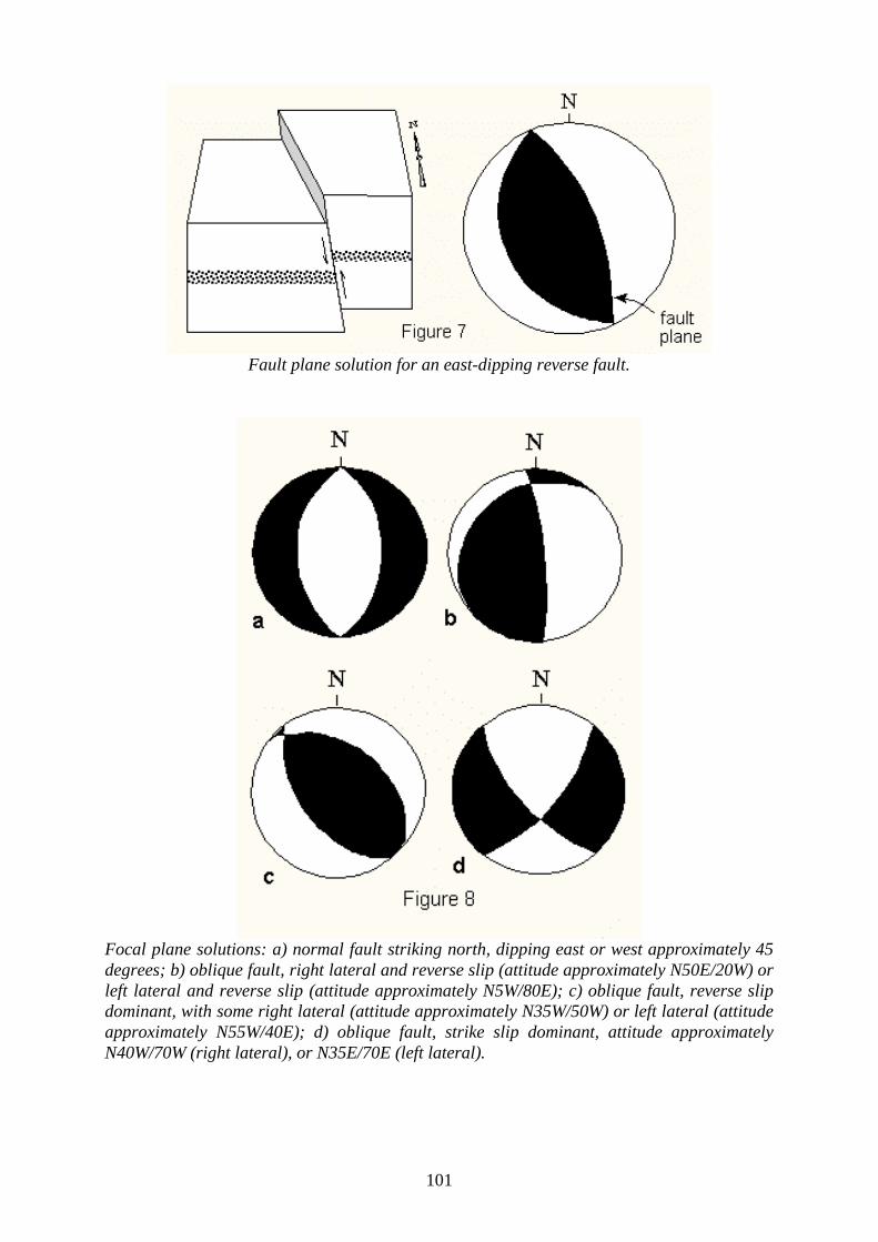
101

Fault plane solution for an east-dipping reverse fault.

Focal plane solutions: a) normal fault striking north, dipping east or west approximately 45 degrees; b) oblique fault, right lateral and reverse slip (attitude approximately N50E/20W) or left lateral and reverse slip (attitude approximately N5W/80E); c) oblique fault, reverse slip dominant, with some right lateral (attitude approximately N35W/50W) or left lateral (attitude approximately N55W/40E); d) oblique fault, strike slip dominant, attitude approximately N40W/70W (right lateral), or N35E/70E (left lateral).

102

Seismic tomography Objective: modelli ng the 3-dimensional velocity structure of the Earth from seismic waves. Convection and the release of heat from the Earth's core drives convection to release heat from the mantle. Convection in the mantle drives plate tectonic motions of the sea floor and continents. It is possible to use P waves and S waves traveling through the mantle from earthquakes to map out this convection, much like a hospital CAT scan can map out bones and organs with x-rays. The following figure shows the paths of shear waves created by an earthquake as they travel through the mantle. Their travel time is recorded by seismographs at the surface. The gray-scales of the images represent deviations of shear velocities from expected average velocities of the mantle at a given depth.

The next figure shows a vertical profile of shear wave velocity anomalies of Australia. The craton with its anomalously high velocities underneath the western part of Australia is well resolved.

103

Positive seismic p-wave velocity anomalies in the mantle (image from the Harvard Univ.) A flattened-out mantle is shown from the northwest. The blobs show where colder, denser material is sinking into the mantle. Near the surface, most of the colder material is in the ancient roots of continental cratons. Subducting slabs of oceanic lithosphere also appear, being recycled into the mantle from oceanic trenches.

Negative seismic p-wave velocity anomalies in the mantle (image from the Harvard Univ.). In this view from the southwest the blobs are warmer plumes of less dense material, rising principally into the ocean-ridge spreading centers. A huge plume seems to be feeding spreading at the East Pacific Rise directly from the core.

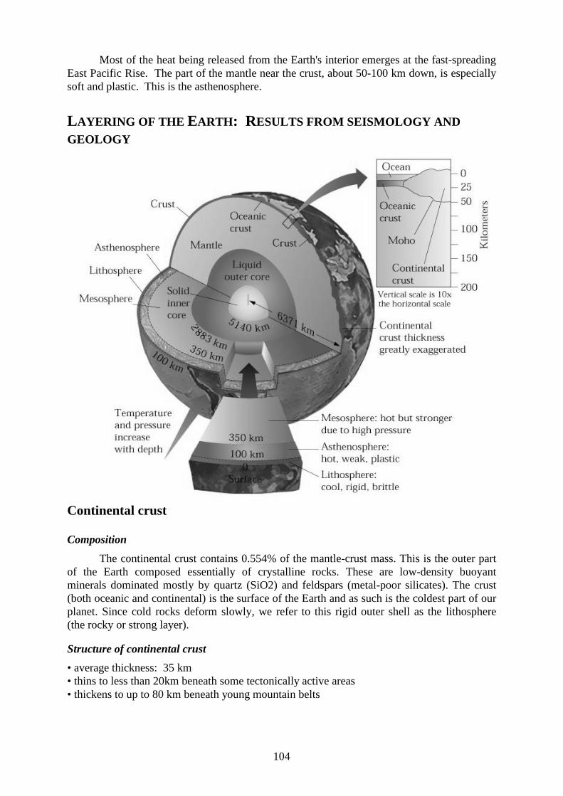
104

Most of the heat being released from the Earth's interior emerges at the fast-spreading East Pacific Rise. The part of the mantle near the crust, about 50-100 km down, is especially soft and plastic. This is the asthenosphere.

LAYERING OF THE EARTH: RESULTS FROM SEISMOLOGY AND GEOLOGY

Continental crust

Composition

The continental crust contains 0.554% of the mantle-crust mass. This is the outer part of the Earth composed essentially of crystalli ne rocks. These are low-density buoyant minerals dominated mostly by quartz (SiO2) and feldspars (metal-poor sili cates). The crust (both oceanic and continental) is the surface of the Earth and as such is the coldest part of our planet. Since cold rocks deform slowly, we refer to this rigid outer shell as the lithosphere (the rocky or strong layer).

Structure of continental crust

• average thickness: 35 km • thins to less than 20km beneath some tectonically active areas • thickens to up to 80 km beneath young mountain belts

105

The boundary between the crust and mantle is called the Mohorovicic discontinuity (or Moho); it is named in honor of the man who discovered it from studies of the seismic waves generated by the Croatia 1909 earthquake, the Croatian scientist Andrija Mohorovicic. No-one has ever seen this boundary, but it can be detected by a sharp increase downward in the speed of earthquake waves there. The explanation for the increase in velocity at the Moho is a change in rock types from crustal to mantle rocks. Drill holes to penetrate the Moho have been proposed, and a Soviet hole on the Kola Peninsula has been drill ed to a depth of 12 kilometers, but drilli ng expense increases enormously with depth, and Moho penetration is not likely very soon.

• another discontinuity was found by Conrad within the crust in 1925, which divides crust into

upper and lower crust • unlike the Moho the Conrad discontinuity is not always present • composition of upper crust: granodiorite and diorite • composition of lower crust: compositionally and structurally complex

Continental crustal thickness (km), compiled by W. Mooney

106

Oceanic crust

Composition

The oceanic crust contains 0.147% of the mantle-crust mass. The majority of the Earth's crust was made through volcanic activity. The oceanic ridge system, a 40,000-km-long network of volcanoes, generates new oceanic crust at the rate of 17 km3 per year, covering the ocean floor with basalt. Hawaii and Iceland are two examples of the accumulation of basalt piles.

Structure of the oceanic crust

• average thickness: 6-7 km • much more homogeneous than continental crust • progressive velocity increase with depth • Layer 1: sediments (average thickness 0.4 km) • Layer 2: basalt (thickness 1-1.5 km) 2a: fractured basalt 2b: massive basalt with sheeted dykes 2c: sheeted dykes with massive basalt • Layer 3: gabbros and metagabbros

Ophiolites

• pieces of ocean crust obducted onto continents • ophiolite = "snake rock" (greek origin) • assoc. of deep sea sediments, basalts, gabbros, and ultrabasic rocks • probably back-arc basin oceanic crust

This is an idealized section of oceanic crust reconstructed from observations of an ophiolite. A thin layer of sediment overlies pillow basalts and a thick pile of gabbro sills. Both the lavas and the sills are intruded by gabbro dikes.

107

Main differences between continental and oceanic crust

Î layering Î thickness Î age Î tectonic activity Î igneous activity

Mantle

Overview

• seismic velocities generally increase with depth • a low-velocity zone is present between 80 and 300km depth • between 400 and 650 km velocity increases stepwise (due to mineral phase changes) • 650 km: lower-upper mantle boundary • Gutenberg discontinuity: core-mantle boundary at a depth of 2885 km • composition: upper mantle: peridotite; lower mantle: perovskite

Seismic discontinuities

Upper mantle: depth of 10-400 km.

The upper mantle contains 15.3% of the mantle-crust mass. Fragments have been excavated for our observation by eroded mountain belts and volcanic eruptions. Olivine (Mg,Fe)2SiO4 and pyroxene (Mg,Fe)SiO3 have been the primary minerals found in this way. These and other minerals are refractory and crystalli ne at high temperatures; therefore, most settle out of rising magma either forming new crustal material or never leaving the mantle. Part of the upper mantle called the asthenosphere may be partially molten.

Transition region: depth of 400-650 km.

The transition region or mesosphere (for middle mantle), sometimes called the fertile layer, contains 11.1% of the mantle-crust mass and is the source of basaltic magmas. It also contains calcium, aluminum, and garnet, which is a complex aluminum-bearing sili cate mineral. This layer is dense when cold because of the garnet and buoyant when hot because these minerals melt easily to form basalt which can then rise through the upper layers as magma.

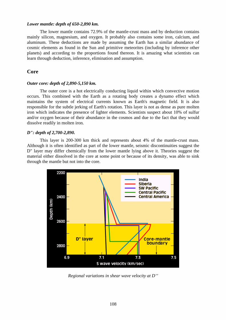
108

Lower mantle: depth of 650-2,890 km.

The lower mantle contains 72.9% of the mantle-crust mass and by deduction contains mainly sili con, magnesium, and oxygen. It probably also contains some iron, calcium, and aluminum. These deductions are made by assuming the Earth has a similar abundance of cosmic elements as found in the Sun and primitive meteorites (including by inference other planets) and according to the proportions found thereon. It is amazing what scientists can learn through deduction, inference, elimination and assumption.

Core

Outer core: depth of 2,890-5,150 km.

The outer core is a hot electrically conducting liquid within which convective motion occurs. This combined with the Earth as a rotating body creates a dynamo effect which maintains the system of electrical currents known as Earth's magnetic field. It is also responsible for the subtle jerking of Earth's rotation. This layer is not as dense as pure molten iron which indicates the presence of lighter elements. Scientists suspect about 10% of sulfur and/or oxygen because of their abundance in the cosmos and due to the fact that they would dissolve readily in molten iron.

D": depth of 2,700-2,890.

This layer is 200-300 km thick and represents about 4% of the mantle-crust mass. Although it is often identified as part of the lower mantle, seismic discontinuities suggest the D" layer may differ chemically from the lower mantle lying above it. Theories suggest the material either dissolved in the core at some point or because of its density, was able to sink through the mantle but not into the core.

Regional variations in shear wave velocity at D’’

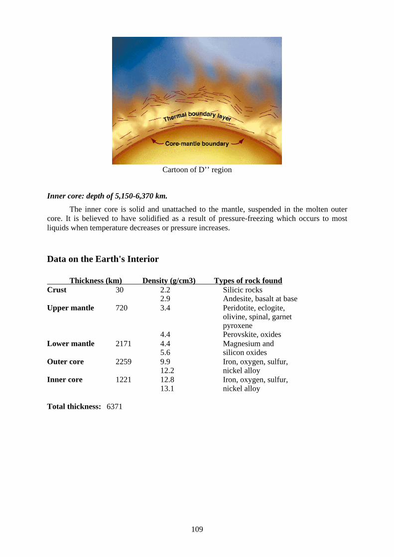
109

Cartoon of D’’ r egion

Inner core: depth of 5,150-6,370 km.

The inner core is solid and unattached to the mantle, suspended in the molten outer core. It is believed to have solidified as a result of pressure-freezing which occurs to most liquids when temperature decreases or pressure increases.

Data on the Ear th's Interior Thickness (km) Density (g/cm3) Types of rock found Crust 30 2.2 Sili cic rocks 2.9 Andesite, basalt at base Upper mantle 720 3.4 Peridotite, eclogite, olivine, spinal, garnet pyroxene 4.4 Perovskite, oxides Lower mantle 2171 4.4 Magnesium and 5.6 sili con oxides Outer core 2259 9.9 Iron, oxygen, sulfur, 12.2 nickel alloy Inner core 1221 12.8 Iron, oxygen, sulfur, 13.1 nickel alloy Total thickness: 6371

110

REFERENCES

Bott, M.H.P., 1993. Modeling the Plate-Driving Mechanism, Journal of the Geological Society, 150: p 941-951.

Bott, M.H.P, 1991. Ridge Push and Associated Plate Interior Stress in Normal and Hot Spot Regions, Tectonophyics, 200: p 17-32.

Bott, M.H.P., 1991. Sublithospheric Loading and Plate-Boundary Forces. In: Whitmarsh, R.B., Bott, M.H.P., Fairhead, J.B. & Kusznir, N.J. (eds) Tectonic Stress in the Lithosphere. Philosophical Transactions of the Royal Society, London, p 83-93.

Carlson, R.L., 1983. Plate Motions, Boundary Forces, and Horizontal Temperature Gradients:Implications for the Driving Mechanism, Tectonophysics, 99: 149-164.

Carlson, R.L, et al., 1983. The Driving Mechanism of Plate Tectonics : Relation to Age of the Lithosphere at Trenches, Geophysical Research Letter, 10: p 297-300.

Chapple, W.M., and Tulli s, T.E., 1977. Evaluation of the Forces that Drive the Plates, Journal of Geophysical Research, 82: p 1967-1984.

Doglioni, C., 1990. The Global Tectonic Pattern. Journal of Geodynamics, 12: p 21-38.

Fleitout, L, 1991. The Sources of Lithosperica Tectonic Stresses. In: Whitmarsh, R.B., Bott, M.H.P., Fairhead, J.B. & Kusznir, N.J. (eds) Tectonic Stress in the Lithosphere. Philosophical Transactions of the Royal Society, London, p 73-81.

Hager, B.H., and O'Connell , R.J., 1978. Subduction Zone Dip Angles and Flow Driven by Plate Motion, Tectonophysics, 50: p 111-133.

Jacoby, W.R., 1980. Plate Sliding and Sinking in Mantle Convection and the Driving Mechaism, In:

Davis, P.A., Runcorn, F.R.S. (eds) Mechanisms of Continental Drift and Plate Tectonics, Academic Press : p 159-172.

Jurdy, D.M., and Stefanick, M., 1991. The Forces Driving the Plates: Constraints from Kinematics and Stress Observations. In: Whitmarsh, R.B., Bott, M.H.P., Fairhead, J.B. & Kusznir, N.J. (eds) Tectonic Stress in the Lithosphere. Philosophical Transactions of the Royal Society, London, p 127-139.

McKenzie, D.P., 1969. Speculations on the Consequences and Causes of Plate Motions, The Geophysical Journal, 18: 1-32.

McKenzie, D.P., 1968. The Influence of the Boundary Conditions and Rotation on Convection in the Earth's Mantle, The Geophysical Journal, 15: 457-500

Middleton, G.V., Wilcock, P.R., 1996. Mechanics in the Earth and Environmental Sciences. Cambridge University Press, Australia : pp 496.

Pavoni, N., 1993. Pattern of Mantle Convection and Pangaea Break-up, as revealed by the evolution of the African plate, Journal of Geological Society, 150: p 953-964.

Richardson, R.M., 1992. Ridge Forces, Absolute Plate Motions, and the Intraplate Stress Field, Journal of Geophysical Research, 97: 11,739-11,748.

111

Runcorn, S.K., 1980. Some Comments on the Mechanism of Continental Drift, In: Davis, P.A., Runcorn,

F.R.S. (eds) Mechanisms of Continental Drift and Plate Tectonics, Academic Press : p 193-198.

Vigny, C., et al., 1991. The Driving Mechanism of Plate Tectonics, Tectonophysics, 187: p 345-360.

Wilson, M., 1993. Plate-moving Mechanisms: Constraints and Controversies, Journal of the Geological Society, 150: p 923-926.

Wilson, M., 1993. Geochemical Signatures of Oceanic and Continental Basalts: A Key to Mantle Dynamics, Journal of Geological Society, 150: p 977-990.

Wortel, M.J.R, et al., 1991. Dynamics of the Lithosphere and the Intraplate Stress Field. In: Whitmarsh, R.B., Bott, M.H.P., Fairhead, J.B. & Kusznir, N.J. (eds) Tectonic Stress in the Lithosphere. Philosophical Transactions of the Royal Society, London, p 111-126.

Wortel, M.J.R., and Vlaar, N.J., 1976. Lithospheric Aging, Instability and Subduction, Tectonophysics, 32: p 331-351.

Ziegler, P.A., 1992. Plate Tectonics, Plate Moving Mechanisms and Rifting, Tectonophysics, 215: p 9-34.

Ziegler, P.A., 1993. Plate-moving Mechanisms: their Relative Importance, Journal of Geological Society, 150: p 927-940

Zoback, M.L., 1992. First and Second Order Patterns of Stress in the Lithosphere: The World Stress Map Project, Journal of Geophysical Research, 97: p 11,703-11,728.

Zoback, M.L., and Magee, M., 1991. Stress Magnitudes in the Crust: Constraints from Stress Orientation and Relative Magnitude Data. In: Whitmarsh, R.B., Bott, M.H.P., Fairhead, J.B. & Kusznir, N.J. (eds) Tectonic Stress in the Lithosphere. Philosophical Transactions of the Royal Society, London, p 181-194.

Zoback, M.L., et al., 1989. Global Patterns of Tectonic Stress, Nature, 341: p 291-298.

112