Deep Learning and Visualizationof Election Data

Garcia, Jorge A.New Mexico State University

Tao, Ng ChingCity University of Hong Kong

Betancourt, FrankUniversity of Tennessee, Knoxville

Wong, KwaiJoint Institute for Computational Sciences

University of Tennessee, Knoxville

(Dated: August 3, 2018)

This paper explores the feasibility of using a Deep Neural Network to predict

bipartisan elections in the US and Hong Kong. Use of political opinion surveys

allows for the training and testing of machine learning models, while predicting

with census data. Statistical analysis of the data then provides various relationships

between electoral parameters that can be visualized.

I. INTRODUCTION

Predicting the outcome of elections, be it at the state or national level, is not a new

idea. Two popular methods used currently are disaggregation and multi-level regression and

poststratification (MRP). As discussed by Lax and Phillips, disaggregation consists of of

calculating the opinion percentages per state, and only requires a respondents answer and

their state of residence [1]. MRP on the other hand is a simulation for a state’s opinion as

a function of demographic and geographic parameters. It is a more generalized and stable

approach in most cases than that of disaggregation [2].

This leads to the question of whether elections can be predicted with Neural Networks

using political opinion surveys. The crucial aspect of political opinion surveys is the fact

that citizens state who they intend to vote for in the upcoming elections. This is what gives

insight as to how a certain region’s results are going to swing. A network could then ”learn”

how certain types of people vote.

2

Neural networks have been around for quite a while, with their mathematical models

dating back to the 1940s [3]. They were largely ignored due to their slow computations and

inaccuracy, but have grown considerably popular in recent years. This is due to the speed

of modern machines and the ability to accumulate very large sets of data (”big data”) that

allow proper training of the networks.

Hong Kong and the United States were chosen since they present a similar, bipartisan

government. America’s political battle between Republicans and Democrats is mimicked

in Hong Kong, with two large coalition of parties known as the Pro-Government and the

Pro-Choice camps. This is allows to ”ask” a question that machine learning algorithms can

predict for easily: binary classification. Both also have a legislative body that is elected by

citizens residing within a certain region; in the United States this is the House of Repre-

sentatives, and its Hong Kong counterpart is the Legislative Council. The 2016 elections of

these are to be predicted.

The following sections will discuss the selection and processing of the data used, the

approach taken to the prediction of election results, and finally the work being done to

visualize the data.

II. HONG KONG LEGISLATIVE COUNCIL

The Legislative Council of Hong Kong Special Administrative Region was established in

1998 with compliance of the Hong Kong Basic Law. The first meeting was held on July 2nd

of that year, with two year terms of for members. Starting from 2000, the term of office was

extended to four years. A new constitutional reform package was introduced in 2012 which

increased the number of members from 60 to 70 for the upcoming election. The duties of

council members include approving the local governments budget and public expenditure,

and discussing issues that involve public interest.

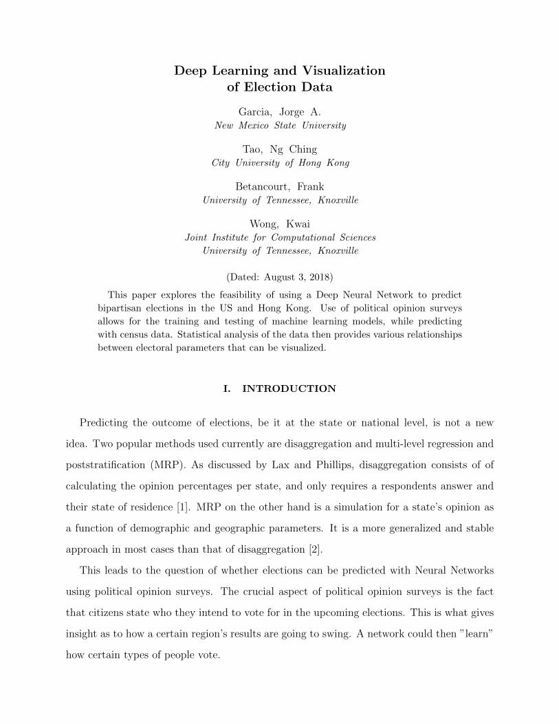
The Hong Kong Legislative Council has two parts, which are Geographical constituency

and Functional constituency. There are five areas under Geographical constituency: Hong

Kong Island, Kowloon West, Kowloon East, New Territories West, and New Territories East,

3

FIG. 1. Distribution of seats of Hong Kong Legislative Council Election

with their seats depending on their population. Like most democracies, people aged eighteen

or above can vote for candidates in their respective district. The total number of seats are

35 for this constituency, with their division determined by the population in each of the five

areas.

The functional constituencies represent various social and economic sectors of the city,

such as Education, Health Services, Labour, etc. Only citizens with occupations related to

the constituency are eligible to vote in it (eg., a medical doctor can vote in the Medical

constituency). There are in total 30 seats for these constituencies. There is also the second

district council functional constituency, in which the rest of the population that can’t vote

in the specialized ones elect 5 more representatives.

Data on the functional constituencies is too sparse for use in deep learning, so they are

not taken into account in this project.

III. UNITED STATES HOUSE OF REPRESENTATIVES

The United States Congress is composed of two chambers, upper and lower, which are

the Senate and the House of Representatives respectively. The number of seats in the House

of Representatives is determined by the population of the states according to the US Census

Bureau. Selection to analyze House elections is due to its similarity to the Legislative Council

in its function and organization.

4

IV. DATA AND PREPROCESSING

The data sets used are free resources, readily available for the public. These include

political opinion surveys, which are used to train and test the Neural Network, and census

population surveys to do predictions.

A. Hong Kong

Analysis of Hong Kong elections is entirely based off the Hong Kong University Public

Opinion Programme’s (HKUPOP) Legislative Council Election Surveys Dataset1. These

surveys asked typical demographic questions (age, occupation, education, etc.), as well as

more subjective matters such as the respondent’s political inclination, or how strongly they

felt about voting.

Since the objective is to predict how the elections are going to fare, it makes most sense

to only use the rolling polls in the model prediction and training, as this is going to be

the obtainable data before elections take place. The surveys are from 2008, 2012 and 2016,

which together total 42177 responses for analysis.

Using the R programming language, the Pearson correlation coefficient is calculated to

quantify how certain factors affect election results. As analyzed from the correlation, political

inclination and education level are the dominant factors affecting the election results. The

complete table with the correlation values can be found in Append ###

Despite being from the same institution, the surveys had different answer keys for the

same question throughout the years used. There was also a number of questions that weren’t

present in other years, leading to the final data set being restricted to only parameters present

in all years. This results with only 9 available parameters to use among the three survey

years, which had to be modified to have similar keys. The loss in number of parameters is

a worthwhile trade though, as it allows to have one large data set instead of 3 smaller and

isolated ones.

1 HKUPOP Data: http://data.hkupop.hku.hk/v2/hkupop/lc_election/en.html

5

A search for census data was done, but no public-use resources are freely available. This

greatly restricts the options to approach the prediction of election outcomes for Hong Kong.

The decided experiment was then to use the surveys from 2008 and 2012 to train the model,

while using the 2016 survey to predict the results of that year’s elections. This was also a

good opportunity though, as, to contrast with the US predictions, it allowed the prediction

to take into account parameters with more subjective matters, such as political inclination.

B. United States

In the case of the US, the political opinion surveys are provided by the American National

Election Studies’ (ANES) Time Series Study2. The data ranges from 1942 to 2016, but that

is a large time span in terms of American politics.Therefore, only data from 1992, right

before President Clinton’s election, was determined to be the start of the current political

climate in order to observe similar voting behavior in individuals with similar demographic

and geographic characteristics. The last year to be taken into account was 2014, as the 2016

data was available after the elections had taken place. While there are over 900 parameters

available in the survey per respondent, only 10 demographic parameters were used since they

had identical counter parts in the census data, presented below.

For use in predictions, the US Census Bureau’s American Community Survey3 (ACS) pro-

vides a representative sample of the population of the state. The respondents are weighted

to represent a certain number of people within the state based on their demographic param-

eters, which easily allows to establish a pool of eligible-voters within the state. Since the

process of accumulating data is a year-round endeavor, the most sensible approach is to use

the survey of the year previous to that of the election. In the case of predicting 2016 results,

use was made of the 2015 survey.

As an initial test, 5 states were chosen: California, Texas, Alabama, Minnesota and

Florida. California and Texas are of the most populated states and are consistent in their

2 ANES Data: https://electionstudies.org/data-center/3 US Census Bureau ACS Data: https://www.census.gov/programs-surveys/acs/

6

political alignment, which makes them a good control group. Alabama and Minnesota are

smaller states with similar sized populations, and also consistent in their alignment, a second

control group. A usual swing state like Florida was chosen to see how the model would predict

as well.

C. Preprocessing

The surveys are all composed in the same fashion. Each parameter represents a ques-

tion asked to the respondent, and the number represents which answer they chose. It was

necessary then to homogenize the data from the surveys into a single format that could be

manipulated as a whole. Using the variable dictionaries provided with the survey by each

organization, Python scripts would go through every element in each survey and replace its

old value with that of the new key.

This was straight forward with most variables: identifying what a certain value means

and matching it to its corresponding value in the other survey’s key. But some parameters

did require an extra amount of work.

1. Ages

For both surveys, it was best to use age groups instead of actual age values. This was

as to simplify the parameter for the model to determine the case of whether a person was

young, middle aged or elderly.

Hong Kong’s age groups are divided from 18-29, 40-59 and 50 and above. This was simply

because it was the simplest of the groupings available in the 2016 survey, and the previous

two were changed to match it.

In the US, they were divided into subgroups of those used by the US Census Bureau. The

groups are from 18-34, 35-64 and 65 and above.

7

2. HK: Ideological Camp

With how elections in Hong Kong are set up, there are various listings from various parties

to choose from. Some regions can even have over 20 different listings. In order to reduce

the output to a binary situation (Pro-Government or Pro-Choice), grouping of the parties to

their respective camp was required. This also removes the worry of having to keep tracking

what listing number a party is throughout the regions and years, and the dominant camp

for the Geographical constituency can be determined.

3. US: Income Group

The ANES Time Series contained information about the respondent’s income group per-

centile, an important factor to consider, especially when shared parameters between the

surveys is limited. The ACS census data contained a person’s income as well, but as a

numerical quantity in actual dollars.

The quickest way to determine the corresponding percentile of a certain income was by

interpolating the information. Using the US Census Bureau’s Income and Poverty in the

United States report for that year, it was possible to find the corresponding income for a

certain percentile, as seen in Table I.

Percentiles Dollars10th 13,25920th 22,80040th 43,51150th 56,51660th 72,00180th 117,00290th 162,18095th 214,462

TABLE I. US income percentiles and their corresponding income for 2015

Using Lagrangian interpolation, a polynomial was generated to approximate the curve

going through the points, resulting in a function that calculates a dollar-value income based

on a percentile. This was necessary due to the ANES survey having specific percentile ranges,

8

such as 17th to 33rd percentile. After determining the percentile of the individual, returning

the categorical value of that range is trivial.

4. One Hot Encoding

Simply feeding the numbers as they are would be assuming they are cardinal or ordinal

numbers, but that is not the case. In order to keep the data having a nominal meaning, it

was necessary to one hot encode (OHE) it so that the network would not consider the real

value of the parameter, but only its existence (See Figure 2). This is also required of output

data for training purposes.

2→[0 0 1 0 0

]FIG. 2. Example of OHE a value of 2, assuming zero-based index.

This way the Neural Network is able to distinguish only whether a possible answer to a

parameter is ”on” (corresponding to the 1) or ”off” (corresponding to the 0). While this

approach increases the dimension of the input parameters by an order of magnitude, this is

not enough to cause problems in the stability of the network’s prediction.

Generation of the input matrix is then done by concatenating all the encoded parameters

for an individual, and stacking all individuals of the survey. In the case of the training data,

the same must be done for an output matrix. At this point then, the data is organized and

ready to be fed into a Neural Network.

V. PREDICTION OF ELECTION OUTCOMES

A Neural Network can be summarized as a multi-dimensional optimization problem. Sup-

pose m is the number of input parameters and k the number of possible outputs. The idea is

that given certain input vector ~x, it is possible to find a function F (~x) that is able to predict

its corresponding output vector ~y, with ~x ∈ Rm and ~y ∈ Rk. In the case of classification,

9

the elements of ~y would be the probability of the input being that class index.

The Keras library for Python 3.x was used to implement the Neural Network. It allows

for quick and easy implementation of a model, allowing the majority of time to be dedicated

to the data and the results.

One approach to the prediction is to only consider individuals who stated who they voted

for in the congress elections. This cuts the training sample in half (many people don’t like

to answer questions of such type), and the model would attempt to predict which of the two

parties the individual would vote for. The activation function to be used would then be the

sigmoid function (Equation 5.1).

f(z) =1

1 + e−z(5.1)

The other possibility is not only attempting to predict what party an individual will vote

for, but whether he will vote or not in the first place. The model’s predictions would then

include the probabilities of no vote and those of voting for one of the parties. The appropriate

activation function for this case is then the softmax function (Equation 5.2).

f(zj)j =ezj∑Ni=1 e

zi(5.2)

Both approaches were tested by setting a RNG seed (since the weights are randomly ini-

tialized) and varying the hyperparameters of various machine learning algorithms in order to

find the optimal approach to election prediction. Figure 3 shows the results of these tests. K

Nearest Neighbors and Random Forest are popular classifier algorithms and straightforward

to implement, and as such were used as a sort of benchmark; the neural networks outperform

them considerably in both cases. It is also interesting to note the instability of prediction

accuracy when using a multiclass classification model.

The best-case scenario is seen with a Deep Neural Network (Labeled NN 2 Layers in the

Figure) with 10 nodes per hidden layer, returning the highest possible accuracy out of all

the trials. This is the architecture used for the rest of the predictions.

The previous trials were run with a high number of epochs to ensure convergence, but

10

FIG. 3. Comparison of US voter prediction accuracy of various machine learning algorithms.

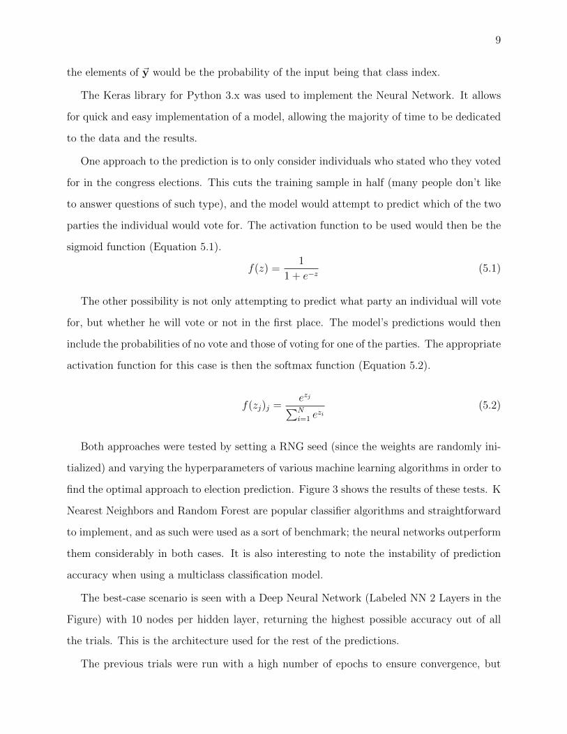
this is not necessary for actual predictions. Figure 4 shows the loss per epoch of the model

in both the US and Hong Kong. Diminishing returns are noticeable at around 15 epochs,

any more would be unnecessary time spent training.

Establishing a performance of the results involved using a prediction as a sort of measure-

ment, since the randomized weights lead to the optimizer converging differently each time.

Various models would be initialized, trained with the political opinion surveys of previous

years, tested with the political opinion survey of the election year and then predicted a result

using the appropriate data set. Finding the appropriate distribution that the sample follows

then allows to calculate the appropriate mean and variance, determining the model’s overall

performance.

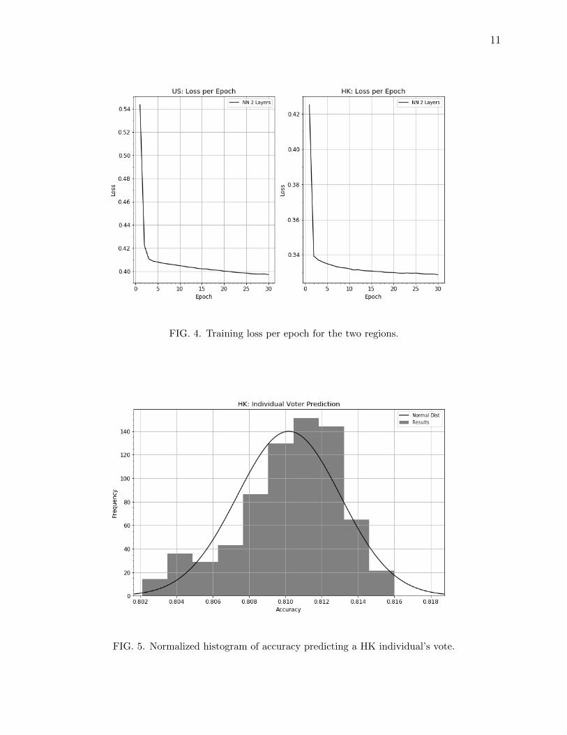
Figures 5 and 6 are the samples of the prediction accuracy of the model for Hong Kong

and the US correspondingly. Hong Kong’s higher accuracy is most likely due to the inclusion

of parameters that go beyond demographics and take a closer look into the individual.

The model is currently only aimed at calculating the popular vote in a state, since this is

11

FIG. 4. Training loss per epoch for the two regions.

FIG. 5. Normalized histogram of accuracy predicting a HK individual’s vote.

12

FIG. 6. Normalized histogram of accuracy predicting a US individual’s vote.

a close representation of a state’s dominant party in congress.

A. Counting Votes

Not all eligible voters participate in elections. Since the model cannot determine whether

an individual will vote or not in the first place, it is possible to take into account voter

turnout to modify the statistical weight of respondents. This allows the model to achieve a

closer approximation of the actual election in both number of votes and outcome.

It is best to use a previous year’s turnout with similar conditions. For example, the 2016

House of Representative Elections took place at the same time the presidential election.

Voter turnout is higher in these years4, as seen in Figure 7, which may impact the other

elections taking place.

For 2016 elections, the most appropriate turnout to use would then be that of 2012

elections. The most simple way to implement this approach would be just taking into

4 US Census Bureau: https://www.census.gov/topics/public-sector/voting/data/tables.All.html

13

FIG. 7. US voter turnout throughout the years. The red bars are years with presidential elections.

account the most diverse turnout category. In the case of the US, it is the racial turnout for

each state that presents the most differences between its groups. They can be observed in

Table II.

State White Hispanic Black AsianTX 60.9% 38.8% 63.1% 42.4%CA 64.3% 48.5% 61.1% 48.6%FL 61.9% 62.2% 57.6% 43.0%MN 74.5% 45.7% 62.1% 78.1%AL 62.0% 48.0% 63.1% 47.9%

TABLE II. US racial turnout for 2012 elections.

These turnouts then act as an extra ”weight” for the statistical weight of an individual

in the census. If, for example, an individual is white and represents 1,600 people within the

state of Texas, then it’s assumed only 60.9% of them participated in the elections. That

individual’s new weight would be of 1600 · 0.609 = 974.4 . This then is the number of votes

this individual is worth.

Since the model returns probabilities of an individual voting for one party or the other,

14

it was decided to adopt a winner-takes-all system. The party with the highest probability

is given the entirety of the votes for that specific individual. The sum of all the weights of

individuals voting for a party would be then be the total number of votes for that party,

and the sum of all weights the number of voters within the selected region. The appropriate

percentage can then be calculated.

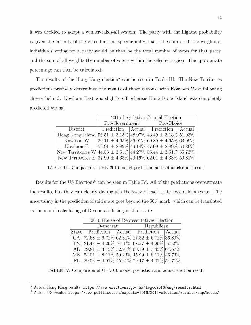
The results of the Hong Kong election5 can be seen in Table III. The New Territories

predictions precisely determined the results of those regions, with Kowloon West following

closely behind. Kowloon East was slightly off, whereas Hong Kong Island was completely

predicted wrong.

2016 Legislative Council ElectionPro-Government Pro-Choice

District Prediction Actual Prediction ActualHong Kong Island 56.51 ± 3.13% 48.97% 43.49 ± 3.13% 51.03%

Kowloon W 30.11 ± 4.65% 36.91% 69.89 ± 4.65% 63.09%Kowloon E 52.91 ± 2.89% 49.14% 47.09 ± 2.89% 50.86%

New Territories W 44.56 ± 3.51% 44.27% 55.44 ± 3.51% 55.73%New Territories E 37.99 ± 4.33% 40.19% 62.01 ± 4.33% 59.81%

TABLE III. Comparison of HK 2016 model prediction and actual election result

Results for the US Elections6 can be seen in Table IV. All of the predictions overestimate

the results, but they can clearly distinguish the sway of each state except Minnesota. The

uncertainty in the prediction of said state goes beyond the 50% mark, which can be translated

as the model calculating of Democrats losing in that state.

2016 House of Representatives ElectionDemocrat Republican

State Prediction Actual Prediction ActualCA 72.68 ± 6.72% 62.31% 27.32 ± 6.72% 36.89%TX 31.43 ± 4.29% 37.1% 68.57 ± 4.29% 57.2%AL 39.81 ± 3.45% 32.91% 60.19 ± 3.45% 64.67%MN 54.01 ± 8.11% 50.23% 45.99 ± 8.11% 46.73%FL 29.53 ± 4.01% 45.21% 70.47 ± 4.01% 54.71%

TABLE IV. Comparison of US 2016 model prediction and actual election result

5 Actual Hong Kong results: https://www.elections.gov.hk/legco2016/eng/results.html6 Actual US results: https://www.politico.com/mapdata-2016/2016-election/results/map/house/

15

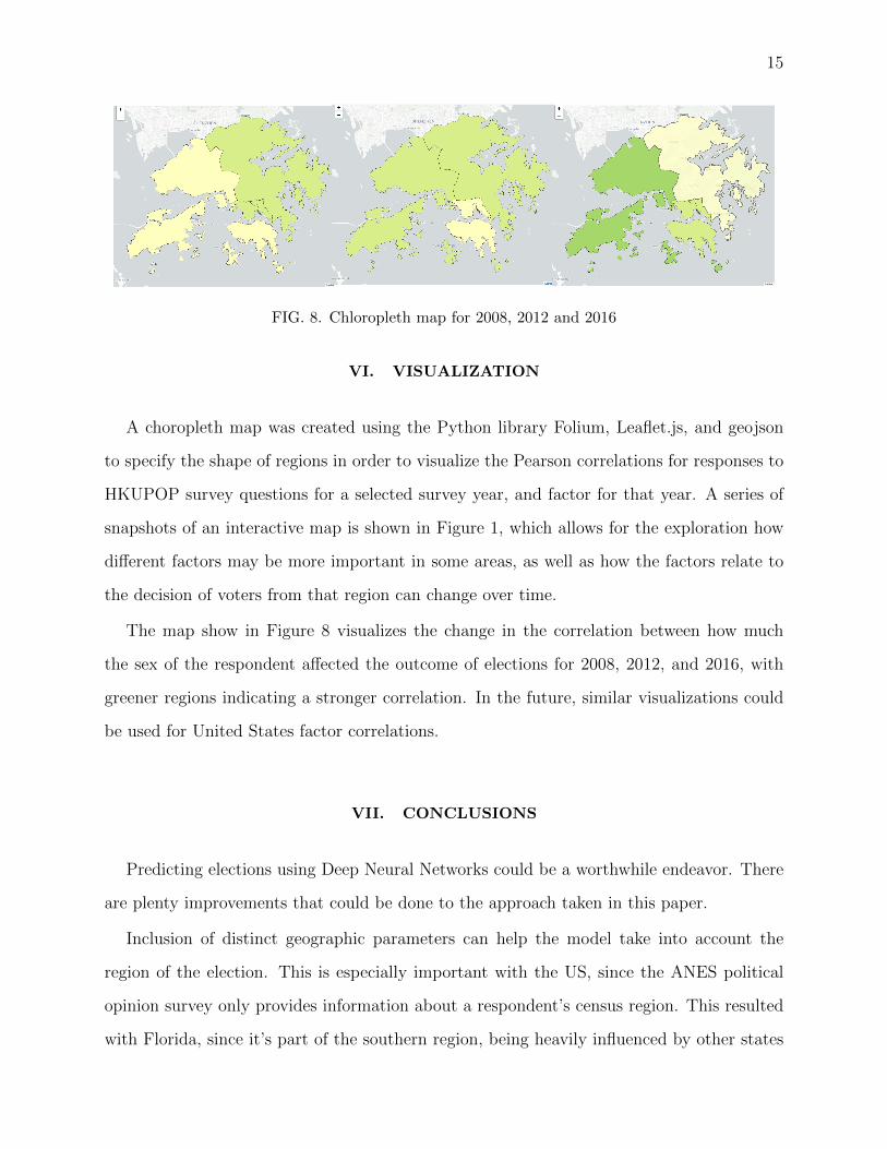
FIG. 8. Chloropleth map for 2008, 2012 and 2016

VI. VISUALIZATION

A choropleth map was created using the Python library Folium, Leaflet.js, and geojson

to specify the shape of regions in order to visualize the Pearson correlations for responses to

HKUPOP survey questions for a selected survey year, and factor for that year. A series of

snapshots of an interactive map is shown in Figure 1, which allows for the exploration how

different factors may be more important in some areas, as well as how the factors relate to

the decision of voters from that region can change over time.

The map show in Figure 8 visualizes the change in the correlation between how much

the sex of the respondent affected the outcome of elections for 2008, 2012, and 2016, with

greener regions indicating a stronger correlation. In the future, similar visualizations could

be used for United States factor correlations.

VII. CONCLUSIONS

Predicting elections using Deep Neural Networks could be a worthwhile endeavor. There

are plenty improvements that could be done to the approach taken in this paper.

Inclusion of distinct geographic parameters can help the model take into account the

region of the election. This is especially important with the US, since the ANES political

opinion survey only provides information about a respondent’s census region. This resulted

with Florida, since it’s part of the southern region, being heavily influenced by other states

16

with deep conservative roots, even though the state of Florida does not share these traits.

Voter turnout consideration could also be an area to improve in. Taking into account

other parameters of a respondent, such as age and sex (there are also different turnouts

between these categories), can result in a more precise voter count, and therefore affecting

the prediction.

More importantly, this approach should be tested against methods such as disaggregation

and multi-level regression and poststratification, Perhaps implementing considerations that

said methods use could result in new possibilities in the field of electoral predictions.

[1] Jeffrey R. Lax and Justin H. Phillips, “How Should We Estimate Public Opinion in The States?”

American Journal of Political Science 53, 107–121 (2009).

[2] Jeffrey R. Lax and Justin H. Phillips, “Estimating state public opinion with multi-level regres-

sion and poststratification using R,” Unpublished manuscript (2010).

[3] Richard P. Lippmann, “An Introduction to Computing with Neural Nets,” IEEE ASSP Maga-

zine 4, 4–22 (1987).

[4] Chad P. Kiewiet de Jonge and Gary Langer, “Predicting 2016 State Presidential Election Results

with a National Tracking Poll and MRP,” Langer Research Associates (2017).

[5] Yair Ghitza and Andrew Gelman, “Deep Interactions with MRP: Election Turnout and Voting

Patterns Among Small Electoral Subgroups,” American Journal of Political Science 57, 762–776

(2017).

[6] Wei Weng, David Rothschild, Sharad Goel, and Andrew Gelman, “Forecasting elections with

non-representative polls,” International Journal of Forecasting 31, 980–991 (2014).