Embed Size (px)
Citation preview

Deep Learning Architecture Searchby Neuro-Cell-based Evolution
with Function-Preserving Mutations
Martin Wistuba
Abstract. The design of convolutional neural network architectures fora new image data set is a laborious and computational expensive taskwhich requires expert knowledge. We propose a novel neuro-evolutionarytechnique to solve this problem without human interference. Our methodassumes that a convolutional neural network architecture is a sequenceof neuro-cells and keeps mutating them using function-preserving op-erations. This novel combination of approaches has several advantages.We define the network architecture by a sequence of repeating neuro-cells which reduces the search space complexity. Furthermore, these cellsare possibly transferable and can be used in order to arbitrarily extendthe complexity of the network. Mutations based on function-preservingoperations guarantee better parameter initialization than random initial-ization such that less training time is required per network architecture.Our proposed method finds within 12 GPU hours neural network ar-chitectures that can achieve a classification error of about 4% and 24%with only 5.5 and 6.5 million parameters on CIFAR-10 and CIFAR-100,respectively. In comparison to competitor approaches, our method pro-vides similar competitive results but requires orders of magnitudes lesssearch time and in many cases less network parameters.
Keywords: Automated Machine Learning · Neural Architecture Search· Evolutionary Algorithms.
1 Introduction
Deep learning techniques have been the key to major improvements in machinelearning in various domains such as image and speech recognition and machinetranslation. Besides more affordable computational power, the proposal of newkinds of architectures such as ResNet [8] and DenseNet [9] helped to increasethe accuracy. However, the selection on which architecture to choose and how towire different layers for a particular data set is not trivial and demands domainexpertise and time from the human practitioner.
Within the last one or two years we observed an increase in research effortsby the machine learning community in order to automate the search for neuralnetwork architectures. Researchers showed that both, reinforcement learning [31]

2 Martin Wistuba
and neuro-evolution [20], are capable of finding network architectures that arecompetitive to the state-of-the-art. Since these methods still require GPU yearsuntil this performance is reached, further work has been proposed to significantlydecrease the run time [1, 3, 15,30,32].
In this paper, we want to present a simple evolutionary algorithm which re-duces the search time to just hours. This is an important step since now, similarto hyperparameter optimization for other machine learning models, optimizingthe network architecture becomes affordable for everyone. Our presented ap-proach starts from a very simple network template which contains a sequence ofneuro-cells. These neuro-cells are architecture patterns and the optimal patternwill be automatically detected by our proposed algorithm. This algorithm as-sumes that the cell initially contains only a single convolutional layer and thenkeeps changing it by function-preserving mutations. These mutations change thestructure of the architecture without changing the network’s predictions. Thiscan be considered as a special initialization such that the network requires lesscomputational effort for training.
Our contributions in this paper are three-fold:
1. We are the first to propose an evolutionary algorithm which optimizes neuro-cells with function-preserving mutations.
2. We expand the set of function-preserving operations proposed by Chen etal. [4] to depthwise separable convolutions, kernel widening, skip connectionsand layers with multiple in- and outputs.
3. We provide empirical evidence that our method is outperforming many com-petitors within only hours of search time. We analyze our proposed methodand the transferability of neuro-cells in detail.
2 Related Work
Evolutionary algorithms and reinforcement learning are currently the two state-of-the-art techniques used by neural network architectures search algorithms.With Neural Architecture Search [31], Zoph et al. demonstrated in an experi-ment over 28 days and with 800 GPUs that neural network architectures withperformances close to state-of-the-art architectures can be found. In parallel orinspired by this work, others proposed to use reinforcement learning to detectsequential architectures [1], reduce the search space to repeating cells [30,32] orapply function-preserving actions to accelerate the search [3].
Neuro-evolution dates back three decades. In the beginning it focused only onevolving weights [18] but it turned out to be effective to evolve the architectureas well [23]. Neuro-evolutionary algorithms gained new momentum due to thework by Real et al. [20]. In an extraordinary experiment that used 250 GPUsfor almost 11 days, they showed that architectures can be found which providesimilar good results as human-crafted image classification network architectures.Very recently, the idea of learning cells instead of the full network has also beenadopted for evolutionary algorithms [15]. Miikkulainen et al. even propose tocoevolve a set of cells and their wiring [17].

Deep Learning Architecture Search by Neuro-Cell-based Evolution 3
Other methods that try to optimize neural network architectures or theirhyperparameters are based on model-based optimization [7, 14, 22, 26], randomsearch [2] and Monte-Carlo Tree Search [19,27].
3 Function-Preserving Knowledge Transfer
Chen et al. [4] proposed a family of function-preserving network manipulationsin order to transfer knowledge from one network to another. Suppose a teacher
network is represented by a function f(x | θ(f)
)where x is the input of the
network and θ(f) are its parameters. Then an operation changing the networkf to a student network g is called function-preserving if and only if the outputfor any given model remains unchanged:
∀x : f(x | θ(f)
)= g
(x | θ(g)
). (1)
Note that typically the number of parameters of f and g are different. We will usethis approach in order to initialize our mutated network architectures. Then, thenetwork is trained for some additional epochs with gradient-based optimizationtechniques. Using this initialization, the network requires only few epochs beforeit provides decent predictions. We briefly explain the proposed manipulationsand our novel contributions to it. Please note that a fully connected layer is aspecial case of a convolutional layer.
3.1 Convolutions in Deep Learning
Convolutional layers are a common layer type used in neural networks for visualtasks. We denote the convolution operation between the layer input X ∈ Rw×h×i
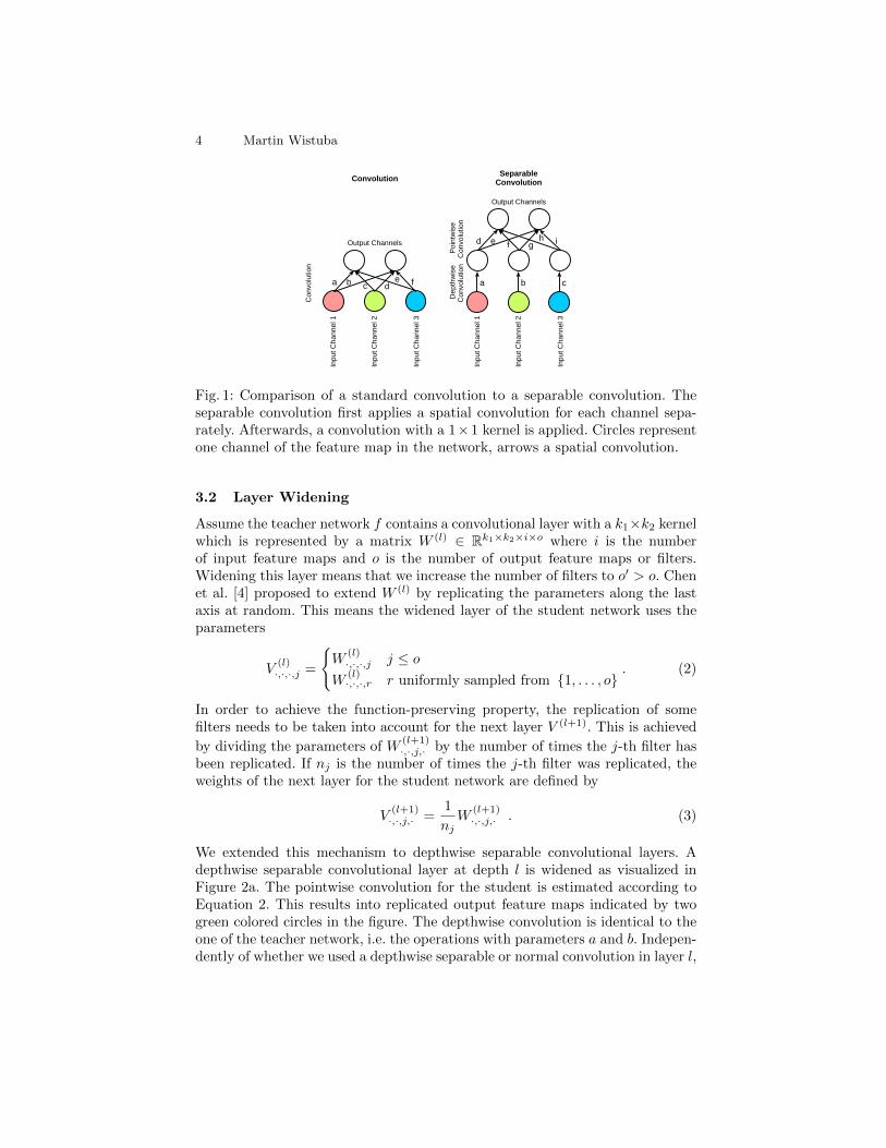
with a layer with parameters W ∈ Rk1×k2×i×o by X∗W . Here, i is the number ofinput channels, w×h the input dimension, k1×k2 the kernel size and o the num-ber of output feature maps. Depthwise separable convolutions, or for short justseparable convolutions, are a special kind of convolution factored into two oper-ations. During the depthwise convolution a spatial convolution with parametersWd ∈ Rk1×k2×i is applied for each channel separately. We denote this operationby using ~. This is in contrast to the typical convolution which is applied acrossall channels. In the next step the pointwise convolution, i.e. a convolution witha 1 × 1 kernel, traverses the feature maps which result from the first operationwith parameters Wp ∈ R1×1×i×o. Comparing the normal convolution operationX ∗W with the separable convolution (X ~Wd) ∗Wp, we immediately noticethat in practice the former requires with k1k2io more parameters than the latterwhich only needs k1k2i+ io. Figure 1 provides a graphical representation of thenetwork. If X(l) is the input for an operation in layer l + 1, e.g. a convolution,
then we represent each channel X(l)·,·,i by a circle. Arrows represent a spatial con-
volution which is parameterized by some parameters indicated by a character(in our example characters a to i). We clearly see that the depthwise convolutionwithin the depthwise separable convolution separately operates on channels andnormal convolutions operate across channels.
4 Martin Wistuba
aba dc b c
Co
nvo
lutio
n
e f
Inp
ut C
han
nel
1
Inp
ut C
han
nel 2
Inp
ut C
ha
nnel
3
Output Channels ed gf
De
pth
wis
eC
on
volu
tion
h i
Inp
ut C
han
nel 1
Inpu
t Cha
nne
l 2
Inp
ut C
han
nel 3
Output Channels
Po
intw
ise
Co
nvo
lutio
n
ConvolutionSeparable
Convolution
Fig. 1: Comparison of a standard convolution to a separable convolution. Theseparable convolution first applies a spatial convolution for each channel sepa-rately. Afterwards, a convolution with a 1×1 kernel is applied. Circles representone channel of the feature map in the network, arrows a spatial convolution.
3.2 Layer Widening
Assume the teacher network f contains a convolutional layer with a k1×k2 kernelwhich is represented by a matrix W (l) ∈ Rk1×k2×i×o where i is the numberof input feature maps and o is the number of output feature maps or filters.Widening this layer means that we increase the number of filters to o′ > o. Chenet al. [4] proposed to extend W (l) by replicating the parameters along the lastaxis at random. This means the widened layer of the student network uses theparameters
V(l)·,·,·,j =
{W
(l)·,·,·,j j ≤ o
W(l)·,·,·,r r uniformly sampled from {1, . . . , o}
. (2)
In order to achieve the function-preserving property, the replication of somefilters needs to be taken into account for the next layer V (l+1). This is achieved
by dividing the parameters of W(l+1)·,·,j,· by the number of times the j-th filter has
been replicated. If nj is the number of times the j-th filter was replicated, theweights of the next layer for the student network are defined by
V(l+1)·,·,j,· =
1
njW
(l+1)·,·,j,· . (3)
We extended this mechanism to depthwise separable convolutional layers. Adepthwise separable convolutional layer at depth l is widened as visualized inFigure 2a. The pointwise convolution for the student is estimated according toEquation 2. This results into replicated output feature maps indicated by twogreen colored circles in the figure. The depthwise convolution is identical to theone of the teacher network, i.e. the operations with parameters a and b. Indepen-dently of whether we used a depthwise separable or normal convolution in layer l,

Deep Learning Architecture Search by Neuro-Cell-based Evolution 5
a b
dc f
g h
e
ji lk
a b
dc f
g h
e
jil/2k/2
df
Sep
ara
ble
Co
nvo
lutio
n
in L
aye
r l
Sep
ara
ble
Co
nvo
lutio
n
in L
aye
r l+
1
Teacher Student
k/2l/2
h
(a) Widening Layer l.
1
Teacher Student
ba dce f
ba dce f
1 1
1 1 10
0
0
000
(b) Insert a separable convolution.
Fig. 2: Visualization of different function-preserving operations. Same coloredcircles represent identical feature maps. Circles without filling can have any valueand are not important for the visualization. Activation functions are omitted toavoid clutter.
widening it requires adaptations in a following depthwise separable convolutionallayer as visualized in Figure 2a. The parameters of the depthwise convolution arereplicated according to the replication of parameters in the previous layer similarto Equation 2. In our example we replicated the operation with parameters f inthe previous layer. Therefore, we have now replicated spatial convolutions withparameters h. Furthermore, the parameter of the pointwise convolution (in theexample parameterized by i, j, k and l) depend on the replications in the previouslayers analogously to Equation 3. In our example we did not replicate the bluefeature map, so the weights for this channel remain unchanged. However, we du-plicated the green feature map which is transformed into the purple feature mapdepthwise convolution. Taking into account that this channel contributes nowtwice to the pointwise convolution, all corresponding weights (in the example kand l) are divided by two.
Widening the separable layer followed by another separable layer is the mostcomplicated case. Other cases can be derived by dropping the depthwise convo-lutions from Figure 2a.
3.3 Layer Deepening
Chen et al. [4] proposed a way to deepen a network by inserting an additionalconvolutional or fully connected layer. We complete this definition by extendingit to depthwise separable convolutions.
A layer can be considered to be a function which gets as an input the outputof the previous layer and provides the input for the next layer. A simple function-preserving operation is to set the weights of a new layer such that the input of

6 Martin Wistuba
the layer is equal to its output. If we assume i incoming channels and an oddkernel height and weight for the new convolutional layer, we achieve this bysetting the weights of the layer with a k1 × k2 kernel to the identity matrix:
V(l)j,h =
{Ii,i j = k1+1
2 ∧ h = k2+12
0 otherwise. (4)
This operation is function-preserving and the number of filters is equal to thenumber of input channels. More filters can be added by layer widening, however,it is not possible to use less than i filters for the new layer. Another restrictionis that this operation is only possible for activation functions σ with
σ (x) = σ (Iσ (x)) ∀x . (5)
The ReLU activation function ReLU (x) = max {x,0} fulfills this requirement.We extend this operation to depthwise convolutions and visualize it in Figure
2b. The parameters of the pointwise convolution Vp are initialized analogouslyto Equation 4 and the depthwise convolution Vd is set to one:
Vp = Ii,i (6)
Vd = 1 . (7)
As we see in Figure 2b, this initialization ensures that both, the depthwise andpointwise convolution, just copy the input. New layers can be inserted at arbi-trary positions with one exception. Under certain conditions an insertion rightafter the input layer is not function-preserving. For example if a ReLU activationis used, there exists no identity function for inputs with negative entries.
3.4 Kernel Widening
Increasing the kernel size in a convolutional layer is achieved by padding thetensor using zeros until it matches the desired size. The same idea can be appliedto increase the kernel size of depthwise separable convolution by padding thedepthwise convolution with zeros.
3.5 Insert Skip Connections
Many modern neural network architectures rely on skip connections [8]. The ideais to add the output of the current layer to the output of a previous. One simpleexample is
X(l+1) = σ(X(l) ∗ V (l+1) +X(l)
). (8)
Therefore, we propose a function-preserving operation which allows insertingskip connection. We propose to add layer(s) and initialize them in a way suchthat the output is 0 independent on the input. This allows to add a skip becausenow adding the output of the previous layer to zero is an identity operation. Wevisualized a simple example in Figure 3a based on Equation 8. A new operationis added setting its parameters to zero, V (l+1) = 0, achieving a zero output.Now, adding this output to the input is an identity operation.

Deep Learning Architecture Search by Neuro-Cell-based Evolution 7
ih kj
Teacher Student
ba dce f ba dc
e f
0 0
00 00
+ +
ih kj
(a) Insert a skip with a convolution.
Teacher Student
hg jik l
badc
e f
hg ji
k
l
1 10 0
badc
e f
(b) Branch the colored layer and insert aconvolution into the left branch.
Fig. 3: Visualization of different function-preserving operations. Same coloredcircles represent identical feature maps. Circles without filling can have any valueand are not important for the visualization. Activation functions are omitted toavoid clutter.
3.6 Branch Layers
We also propose to branch layers. Given a convolutional layer X(l) ∗W (l+1) itcan be reformulated as
merge(X(l) ∗ V (l+1)
1 , X(l) ∗ V (l+1)2
), (9)
where merge concatenates the resulting output. The student network’s parame-ters are defined as
V(l+1)1 = W
(l+1)·,·,·,1:bo/2c
V(l+1)2 = W
(l+1)·,·,·,(bo/2c+1):o .
This operation is not only function-preserving, it also does not add any furtherparameters and in fact is the very same operation. However, combining thisoperation with other function-preserving operations allows to extend networksby having parallel convolutional operations or add new convolutional layers withsmaller filter sizes. In Figure 3b we demonstrate how to achieve this. The coloredlayer is first branched and then a new convolutional layer is added to the leftbranch. In contrast to only adding a new layer as described in Section 3.3, thenew layer has only two output channels instead of three.

8 Martin Wistuba
Conv (64, 3, 3)Cell
Max PoolingCell
Max PoolingCell
Conv (128, 3, 3) FC (128) Softmax
Fig. 4: Neural network template as used in our experiments.
3.7 Multiple In- or Outputs
All the presented operations are still possible for networks where a layer mighthave inputs from different layers or provide output for multiple outputs. In thatcase only the affected weights need to be adapted according to the aforemen-tioned equations.
4 Evolution of Neuro-Cells
The very basic idea of our proposed cell-based neuro-evolution is the follow-ing. Given is a very simple neural network architecture which contains multipleneuro-cells (see Figure 4). The cells itself share their structure and the task isto find a structure that improves the overall neural network architecture for agiven data set and machine learning task. In the beginning, a cell is identicalto a convolutional layer and is changed during the evolutionary optimizationprocess. Our evolutionary algorithm is using tournament selection to select anindividual from the population: randomly, a fraction k of individuals is selectedfrom the population. From this set the individual with highest fitness is selectedfor mutation. We define the fitness by the accuracy achieved by the individualon a hold-out data set. The mutation is selected at random which is applied toall neuro-cells such that they remain identical. The network is trained for someepochs on the training set and is then added to the population. Finally, the pro-cess starts all over again. After meeting some stopping criterion, the individualwith highest fitness is returned.
4.1 Mutations
All mutations used are based on the function-preserving operations introducedin the last section. This means, a mutation does not change the fitness of anindividual, however, it will increase its complexity. The advantage over creatingthe same network structure with randomly initialized weights is obviously thatwe start with a partially pretrained network. This enables us to train the networkin less epochs. All mutations are applied only to the structure within a neuro-cell if not otherwise mentioned. Our neuro-evolutional algorithm considers thefollowing mutations.
Insert Convolution A convolution is added at a random position. Its kernel sizeis 3 × 3, the number of filters is equal to its input dimension. It is randomlydecided whether it is a separable convolution instead.

Deep Learning Architecture Search by Neuro-Cell-based Evolution 9
Branch and Insert Convolution A convolution is selected at random and branchedaccording to Section 3.6. A new convolution is added according to the “InsertConvolution” mutation in one of the branches. For an example see Figure 3b.
Insert Skip A convolution is selected at random. Its output is added to theoutput of a newly added convolution (see “Insert Convolution”) and is the inputfor the following layers. For an example see Figure 3a.
Alter Number of Filters A convolution is selected at random and widened by afactor uniformly at random sampled from [1.2, 2]. This mutation might also beapplied to convolutions outside of a neuro-cell.
Alter Number of Units Similar to the previous one but alters the number of unitsof fully connected layers. This mutation is only applied outside the neuro-cells.
Alter Kernel Size Selects a convolution at random and increases its kernel sizeby two along each axis.
Branch Convolution Selects a convolution at random and branches it accordingto Section 3.6.
The motivation of selecting this set of mutations is to enable the neuro-evolutionary algorithm to discover similar architectures as proposed by hu-man experts. Adding convolutions allows to reach popular architectures suchas VGG16 [21], combinations of adding skips and convolutions allow to discoverresidual networks [8]. Finally the combination of branching, change of kernelsizes and addition of (separable) convolutions allows to discover architecturessimilar to Inception [25], Xception [5] or FractalNet [13].
The optimization is started with only a single individual. We enrich the pop-ulation by starting with an initialization step which creates 15 mutated versionsof the first individual. Then, individuals are selected based on the previouslydescribed tournament selection process.
5 Experiments
In the experimental section we will run our proposed method for the task of imageclassification on the two data sets CIFAR-10 and CIFAR-100. We conduct the fol-lowing experiments. First, we analyze the performance of our neuro-evolutionalapproach with respect to classification error and compare it to various competi-tor approaches. We show that we achieve a significant search time improvementat costs of slightly larger error. Furthermore, we give insights how the evolutionand the neuro-cells progress and develop during the optimization process. Ad-ditionally, we discuss the possibility of transferring detected cells to novel datasets. Finally, we compare the performance of two different random approachesin order to prove our method’s benefit.

10 Martin Wistuba
5.1 Experimental Setup
The network template used in our experiments is sketched in Figure 4. It startswith a small convolution, followed twice by a neuro-cell and a max poolinglayer. Then, another neuro-cell is added, followed by a larger convolution, afully connected layer and the final softmax layer. Each max pooling layer hasa stride of two and is followed by a drop-out layer with drop-out rate 70%.The fully connected layer is followed by a drop-out layer with rate 50%. In thissection, whenever we sketch or mention a convolutional layer, we actually mean aconvolutional layer followed by batch normalization [11] and a ReLU activation.The neuro-cell is initialized with a single convolution with 128 filters and a kernelsize of 3× 3. A weight decay of 0.0001 is used.
We evaluate our method and compare it to competitor methods on CIFAR-10 and CIFAR-100 [12]. We use standard preprocessing and data augmentation.All images are preprocessed by subtracting from each channel its mean anddividing it by its standard deviation. The data augmentation involves paddingthe image to size 40 × 40 and then cropping it to dimension 32 × 32 as well asflipping images horizontally at random. We split the official training partitionsinto a partition which we use to train the networks and a hold-out partition toevaluate the fitness of the individuals.
For the neuro-evolutionary algorithm we select a tournament size equal to15% of the population but at least two. The initial network is trained for 63epochs, every other network is trained for 15 epochs with Nesterov momentumand a cosine learning rate schedule with initial learning rate 0.05, T0 = 1 andTmul = 2 [16]. We define the fitness of an individual by the accuracy of thecorresponding network on the hold-out partition. After the search budget isexhausted, the individual with highest fitness is trained on the full training splituntil convergence using CutOut [6]. Finally, the error on test is reported.
5.2 Search for Networks
In Table 1 we report the mean and standard deviation of our approach acrossfive runs and compare it to other approaches.
The first block contains several architectures proposed by human experts.DenseNet [9] is clearly the best among them, reaching an error of 4.51% withonly 800 thousand parameters. Using about 25 million parameters, the errordecreases to 3.42%.
The second block contains several architecture search methods based on re-inforcement learning. Most of them are able to find very competitive networksbut at the cost of very high search times. NASNet [32] finds the best-performingnetwork which is on par with DenseNet but requires less parameters. However,the authors report that they required about 5.5 GPU years in order to reach thisperformance. Efficient Architecture Search [3] still achieves an error of 4.23% butreduces the search time drastically to ten days.
The third block contains various automated approaches based on evolution-ary methods. Hierarchical Evolution [15] finds the best performing architecture

Deep Learning Architecture Search by Neuro-Cell-based Evolution 11
Table 1: Classification error on CIFAR-10 and CIFAR-100 including spent searchtime in GPU days. The first block presents the performance of state-of-the-arthuman-designed architectures. The second block contains results of various au-tomated architecture search methods based on reinforcement learning. The thirdblock contains results for automated methods based on evolutionary algorithms.The final block presents our results. For our method, we report the mean of fiverepetitions for the classification error and the number of parameters, the bestrun and the run with least network parameters.
Method Duration CIFAR-10 CIFAR-100Error Params Error Params
ResNet [8] reported by [10] N/A 6.41 1.7M 27.22 1.7MFractalNet [13] N/A 5.22 38.6M 23.30 38.6MWide ResNet (depth = 16) [29] N/A 4.81 11.0M 22.07 11.0MWide ResNet (depth = 28) [29] N/A 4.17 36.5M 20.50 36.5MDenseNet-BC (k = 12) [9] N/A 4.51 0.8M 22.27 0.8MDenseNet-BC (k = 24) [9] N/A 3.62 15.3M 17.60 15.3MDenseNet-BC (k = 40) [9] N/A 3.42 25.6M 17.18 25.6M
NAS no stride/pooling [31] 22,400 5.50 4.2M - -NAS predicting strides [31] 22,400 6.01 2.5M - -NAS max pooling [31] 22,400 4.47 7.1M - -NAS max pooling + more filters [31] 22,400 3.65 37.4M - -NASNet [32] 2,000 3.41 3.3M - -MetaQNN [1] 100 6.92 11.2M 27.14 11.2MBlockQNN [30] 96 3.6 ? 18.64 ?Efficient Architecture Search [3] 10 4.23 23.4M - -
Large-Scale Evolution [20] 2,600 5.4 5.4M 23.0 40.4MHierarchical Evolution [15] 300 3.75 15.7M - -CGP-CNN (ResSet) [24] 27.4 6.05 2.6M - -CoDeepNEAT [17] ? 7.30 ? - -
Ours (mean) 0.5 4.02 5.6M 23.92 6.5MOurs (mean) 1 3.89 7.0M 22.32 6.7MOurs (best) 0.5 3.57 5.8M 22.08 6.8MOurs (best) 1 3.58 7.2M 21.74 5.3MOurs (least params) 0.5 4.19 3.8M 28.15 5.0MOurs (least params) 1 3.77 5.8M 21.74 5.3M

12 Martin Wistuba
●● ●●
● ●● ●
●
● ●
● ●
● ●
●
●
●
●
●● ● ●
● ●●
● ●●
●● ● ●
●●
●● ● ● ● ● ●
●
●●
●
●●
●●
●
●
●●
●●
●
●●
●●
●
●●
●●
●
●●
●●
●●
●
●●
●
●●
●●
●
●
●●
●
●
●
●●
0 5 10 15 20
Time in hours
0.825
0.850
0.875
0.900
0.925
Accuracy
Fig. 5: Evolutionary algorithm over time. Each dot represents an individual,connections represent the ancestry. After the initialization, the algorithm quicklyfocuses on ancestors from only one initial individual.
among them in 300 GPU days. Methodologically, our approach also belongs intothis category. We want to highlight in particular the search time required by ourproposed method. Within only 12 and 24 hours, respectively, a network architec-ture is found which gives better predictions than most competitors and is veryclose to the best methods. After 12 hours of search, we report a mean classifica-tion error over five repetitions of 4.02±0.376 and 23.92±2.493 on CIFAR-10 andCIFAR-100, respectively. Extending the search by another 12 hours, the errorreduces to 3.89± 0.231 and 22.32± 0.429.
In order to give insights into the optimization process, we visualized one runon CIFAR-10 in Figure 5 and 6. Figure 5 visualizes the fitness of each individualbut also its ancestry by a phylogenetic tree [28]. The x-axis represents the time,the y-axis has no meaning. The color indicates the fitness, dots represent indi-viduals and the ancestry is represented by edges. We notice that within the first10 hours the fitness is increasing quickly. Afterwards, progress is slow but steady.Figure 6 provides in parallel insight which stages the final neuro-cell underwent.Over time the cell develops multiple computation branches, finally adding someskip connections. Notice, that branching the 7 × 7 convolution as first shownat Hour 19 has no purpose. However, this might have changed for a longer runwhen e.g. another layer was added in one of these branches.
5.3 Neuro-Cell Transferability
An interesting aspect is whether a neuro-cell detected on one data set can bereused in a different architecture and for a different data set. For this reason, weexpanded the template from Figure 4 by duplicating the number of cells to theone shown in Figure 7. We used the cells and other hyperparameters detected inour 12 hours CIFAR-10 experiment and used the resulting networks for imageclassification on CIFAR-100. These models achieved an average error of 24.77%with a standard deviation of 1.61%. This result is not as good as the one achieved

Deep Learning Architecture Search by Neuro-Cell-based Evolution 13
Ho
ur
1F
itnes
s: 0
.881
9
Con
v (1
28,
3, 3
)
Sep
Con
v (1
28,
3, 3
)
Con
v (1
28,
3, 3
)
Con
v (1
28,
3, 3
)
Ho
ur
2F
itnes
s: 0
.88
84
Con
v (1
28,
3, 3
)
Con
v (6
4, 3
, 3)H
ou
r 4
Fitn
ess:
0.9
052
Con
v (6
4, 3
, 3)
Sep
Con
v (1
28, 5
, 5)
Con
v (1
28,
3, 3
)
Con
v (9
2, 3
, 3)H
ou
r 7
Fitn
ess:
0.9
246
Con
v (6
4, 5
, 5)
Con
v (1
56,
3, 3
)
Sep
Con
v (1
28,
5, 5
)
Con
v (1
28, 3
, 3)
Con
v (9
2, 3
, 3)
Ho
ur
10F
itnes
s: 0
.925
1
Con
v (3
2, 7
, 7)
Con
v (1
56, 3
, 3)
Con
v (3
2, 7
, 7)
Con
v (1
28,
3, 3
)
Sep
Con
v (1
28, 5
, 5)
Con
v (1
28,
3, 3
)
Con
v (9
2, 3
, 3)
Ho
ur
13F
itnes
s: 0
.934
7
Con
v (3
2, 7
, 7)
Con
v (1
56,
5, 5
)
Con
v (3
2, 7
, 7)
Con
v (1
28,
3, 3
)
+
Sep
Con
v (1
28,
3, 3
)S
ep C
onv
(128
, 5,
5)
Con
v (1
28,
3, 3
)
Con
v (9
2, 3
, 3)
Ho
ur
19F
itnes
s: 0
.932
3
Con
v (1
56,
5, 5
)
Con
v (1
28,
3, 3
)
+
Sep
Con
v (1
28,
3, 3
)
Sep
Con
v (1
28,
3, 3
)
+
Con
v (1
6, 7
, 7)
Con
v (1
6, 7
, 7)
Con
v (3
2, 7
, 7)
Sep
Con
v (1
28, 5
, 5)
Con
v (1
28,
3, 3
)
Con
v (9
2, 3
, 3)
Ho
ur
21F
itnes
s: 0
.935
7
Con
v (1
56,
5, 5
)
Con
v (1
28,
3, 3
)
+
Sep
Con
v (1
28,
3, 3
)
Sep
Con
v (1
28, 3
, 3)
+
Con
v (1
6, 7
, 7)
Con
v (1
6, 7
, 7)
Con
v (1
28,
3, 3
)
Con
v (1
28,
3, 3
)
Con
v (1
6, 7
, 7)
Con
v (1
6, 7
, 7)
Fig
.6:
Evo
luti
onar
yp
roce
ssof
the
bes
tn
euro
-cel
lfo
und
du
rin
gon
eru
non
CIF
AR
-10.
Som
ein
term
edia
test
ate
sare
skip
ped
.

14 Martin Wistuba
Conv (64, 3, 3)Cell Cell
Max PoolingCell
Conv (128, 3, 3) FC (128) SoftmaxCell
Max PoolingCell Cell
Fig. 7: Expanded template for the neuro-cell transferability experiment.
by searching for the best architecture for CIFAR-100 but therefore no new searchis required for the new data set.
5.4 Random Search
In this section we will discuss the importance of our evolutionary approach bycomparing it to two random network searches.
Comparison to Random Individual Selection Random individual selectionis in fact not really a valid comparison because it is actually a special case ofour proposed method with a tournament size of one. For this experiment, weselect a random individual from the population instead of selecting the bestindividual of a random population subset. With this small change, we run ouralgorithm five times for twelve hours. We report a mean classification error of4.55% with standard deviation 0.34%. Note, that the best of these runs achievedan error of 4.04% which is still worse than the mean error achieved when usinglarger tournament sizes. Thus, we can confirm that tournament selection providesbetter results than random selection.
Comparison to Random Mutations We conduct another experiment wherewe apply k mutations to the initial individual. In practice, k is dependent on thedata set and not known and thus, this method is actually not really applicable.However, for this experiment, we set k to the number of mutations used for thebest cell in our 12 hours experiment. In comparison to the random individualselection, this method further increases the error to 4.73% on average over fiverepetitions with a standard deviation of 0.63%.
6 Conclusions
We proposed a novel approach which optimizes the neural network architecturebased on an evolutionary algorithm. It requires as an input a simple templatecontaining neuro-cells, replicated architecture patterns, and automatically keepsimproving this initial architecture. The mutations of our evolutionary algorithmare based on function-preserving operations which change the network’s archi-tecture without changing its prediction. This enables shorter training times incomparison to a random initialization. In comparison to the state-of-the-art, wereport very competitive results and show outstanding results with respect to the

Deep Learning Architecture Search by Neuro-Cell-based Evolution 15
search time. Our approach is up to 50,000 times faster than some of the competi-tor methods with an error rate at most 0.6% higher than the best competitoron CIFAR-10.
References
1. Baker, B., Gupta, O., Naik, N., Raskar, R.: Designing neural network architecturesusing reinforcement learning. In: Proceedings of the International Conference onLearning Representations, ICLR 2017, Toulon, France, April 24-26 (2017)
2. Bergstra, J., Bengio, Y.: Random search for hyper-parameter optimization. Journalof Machine Learning Research 13, 281–305 (2012)
3. Cai, H., Chen, T., Zhang, W., Yu, Y., Wang, J.: Reinforcement learning for archi-tecture search by network transformation. CoRR abs/1707.04873 (2017)
4. Chen, T., Goodfellow, I.J., Shlens, J.: Net2Net: Accelerating learning via knowl-edge transfer. In: Proceedings of the International Conference on Learning Repre-sentations, ICLR 2016, San Juan, Puerto Rico, May 2-4 (2016)
5. Chollet, F.: Xception: Deep learning with depthwise separable convolutions. CoRRabs/1610.02357 (2016)
6. Devries, T., Taylor, G.W.: Improved regularization of convolutional neural net-works with cutout. CoRR abs/1708.04552 (2017)
7. Diaz, G.I., Fokoue-Nkoutche, A., Nannicini, G., Samulowitz, H.: An effective al-gorithm for hyperparameter optimization of neural networks. IBM Journal of Re-search and Development 61(4), 9 (2017)
8. He, K., Zhang, X., Ren, S., Sun, J.: Deep residual learning for image recognition.In: 2016 IEEE Conference on Computer Vision and Pattern Recognition, CVPR2016, Las Vegas, NV, USA, June 27-30, 2016. pp. 770–778 (2016)
9. Huang, G., Liu, Z., van der Maaten, L., Weinberger, K.Q.: Densely connected con-volutional networks. In: 2017 IEEE Conference on Computer Vision and PatternRecognition, CVPR 2017, Honolulu, HI, USA, July 21-26, 2017. pp. 2261–2269(2017)
10. Huang, G., Sun, Y., Liu, Z., Sedra, D., Weinberger, K.Q.: Deep networks withstochastic depth. In: Computer Vision - ECCV 2016 - 14th European Conference,Amsterdam, The Netherlands, October 11-14, 2016, Proceedings, Part IV. pp.646–661 (2016)
11. Ioffe, S., Szegedy, C.: Batch normalization: Accelerating deep network training byreducing internal covariate shift. In: Proceedings of the 32nd International Confer-ence on Machine Learning, ICML 2015, Lille, France, 6-11 July 2015. pp. 448–456(2015)
12. Krizhevsky, A.: Learning multiple layers of features from tiny images. Tech. rep.(2009)
13. Larsson, G., Maire, M., Shakhnarovich, G.: Fractalnet: Ultra-deep neural networkswithout residuals. In: Proceedings of the International Conference on LearningRepresentations, ICLR 2017, Toulon, France, April 24-26 (2017)
14. Liu, C., Zoph, B., Shlens, J., Hua, W., Li, L., Fei-Fei, L., Yuille, A.L., Huang,J., Murphy, K.: Progressive neural architecture search. CoRR abs/1712.00559(2017)
15. Liu, H., Simonyan, K., Vinyals, O., Fernando, C., Kavukcuoglu, K.: Hierarchicalrepresentations for efficient architecture search. In: Proceedings of the InternationalConference on Learning Representations, ICLR 2018, Vancouver, Canada (2018)

16 Martin Wistuba
16. Loshchilov, I., Hutter, F.: SGDR: Stochastic gradient descent with warm restarts.In: Proceedings of the International Conference on Learning Representations, ICLR2017, Toulon, France, April 24-26 (2017)
17. Miikkulainen, R., Liang, J.Z., Meyerson, E., Rawal, A., Fink, D., Francon, O.,Raju, B., Shahrzad, H., Navruzyan, A., Duffy, N., Hodjat, B.: Evolving deep neuralnetworks. CoRR abs/1703.00548 (2017)
18. Miller, G.F., Todd, P.M., Hegde, S.U.: Designing neural networks using geneticalgorithms. In: Proceedings of the 3rd International Conference on Genetic Algo-rithms, George Mason University, Fairfax, Virginia, USA, June 1989. pp. 379–384(1989)
19. Negrinho, R., Gordon, G.J.: Deeparchitect: Automatically designing and trainingdeep architectures. CoRR abs/1704.08792 (2017)
20. Real, E., Moore, S., Selle, A., Saxena, S., Suematsu, Y.L., Tan, J., Le, Q.V., Ku-rakin, A.: Large-scale evolution of image classifiers. In: Proceedings of the 34thInternational Conference on Machine Learning, ICML 2017, Sydney, NSW, Aus-tralia, 6-11 August 2017. pp. 2902–2911 (2017)
21. Simonyan, K., Zisserman, A.: Very deep convolutional networks for large-scaleimage recognition. CoRR abs/1409.1556 (2014)
22. Snoek, J., Larochelle, H., Adams, R.P.: Practical bayesian optimization of machinelearning algorithms. In: Advances in Neural Information Processing Systems 25:26th Annual Conference on Neural Information Processing Systems 2012. Proceed-ings of a meeting held December 3-6, 2012, Lake Tahoe, Nevada, United States.pp. 2960–2968 (2012)
23. Stanley, K.O., Miikkulainen, R.: Evolving neural networks through augmentingtopologies. Evol. Comput. 10(2), 99–127 (Jun 2002)
24. Suganuma, M., Shirakawa, S., Nagao, T.: A genetic programming approach to de-signing convolutional neural network architectures. In: Proceedings of the Geneticand Evolutionary Computation Conference, GECCO 2017, Berlin, Germany, July15-19, 2017. pp. 497–504 (2017)
25. Szegedy, C., Liu, W., Jia, Y., Sermanet, P., Reed, S.E., Anguelov, D., Erhan,D., Vanhoucke, V., Rabinovich, A.: Going deeper with convolutions. In: IEEEConference on Computer Vision and Pattern Recognition, CVPR 2015, Boston,MA, USA, June 7-12, 2015. pp. 1–9 (2015)
26. Wistuba, M.: Bayesian optimization combined with successive halving for neu-ral network architecture optimization. In: Proceedings of AutoML@PKDD/ECML2017, Skopje, Macedonia, September 22, 2017. pp. 2–11 (2017)
27. Wistuba, M.: Finding competitive network architectures within a day using UCT.CoRR abs/1712.07420 (2017)
28. Yu, G., Smith, D.K., Zhu, H., Guan, Y., Lam, T.T.Y.: ggtree: an R package forvisualization and annotation of phylogenetic trees with their covariates and otherassociated data. Methods Ecol. Evol. 8(1), 28–36 (Jul 2016)
29. Zagoruyko, S., Komodakis, N.: Wide residual networks. In: Proceedings of theBritish Machine Vision Conference 2016, BMVC 2016, York, UK, September 19-22, 2016 (2016)
30. Zhong, Z., Yan, J., Liu, C.: Practical network blocks design with q-learning. CoRRabs/1708.05552 (2017)
31. Zoph, B., Le, Q.V.: Neural architecture search with reinforcement learning. In:Proceedings of the International Conference on Learning Representations, ICLR2017, Toulon, France, April 24-26 (2017)
32. Zoph, B., Vasudevan, V., Shlens, J., Le, Q.V.: Learning transferable architecturesfor scalable image recognition. CoRR abs/1707.07012 (2017)