Embed Size (px)
Citation preview
Attacking Mobile Traffic Analytics and Backhaul Utility Maximisation with Deep Learning
Paul PatrasWork with Chaoyun Zhang, Rui Li, John Thompson (U Edinburgh), Xi Ouyang (Huazhong UST), Pan Cao (U Hertfordshire)
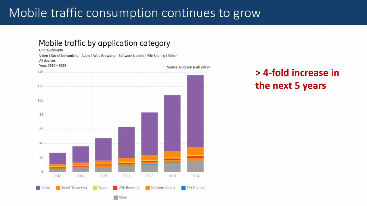
The Goal of Mobile Traffic AnalysisMobile traffic consumption continues to grow
> 4-fold increase in the next 5 years
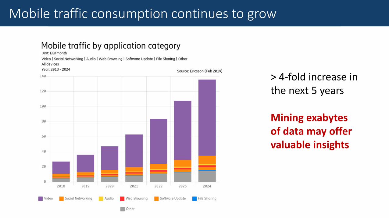
The Goal of Mobile Traffic AnalysisMobile traffic consumption continues to grow
> 4-fold increase in the next 5 years
Mining exabytes of data may offer valuable insights
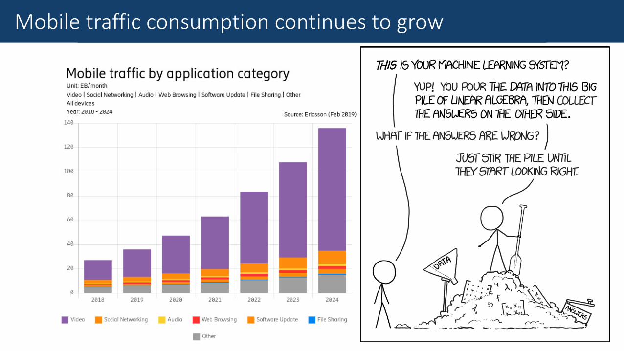
The Goal of Mobile Traffic AnalysisMobile traffic consumption continues to grow

Forecasting future mobile traffic consumption
The Goal of Mobile Traffic Analysis
1. Precision traffic engineering
- On demand allocation of resources
- Building Intelligent 5G networks
2. Energy saving
– Green cellular networks
3. Mobility analysis
- Movement prediction
- Transportation planning
Importance of Precision Mobile Traffic Forecasting
The Goal of Mobile Traffic Analysis
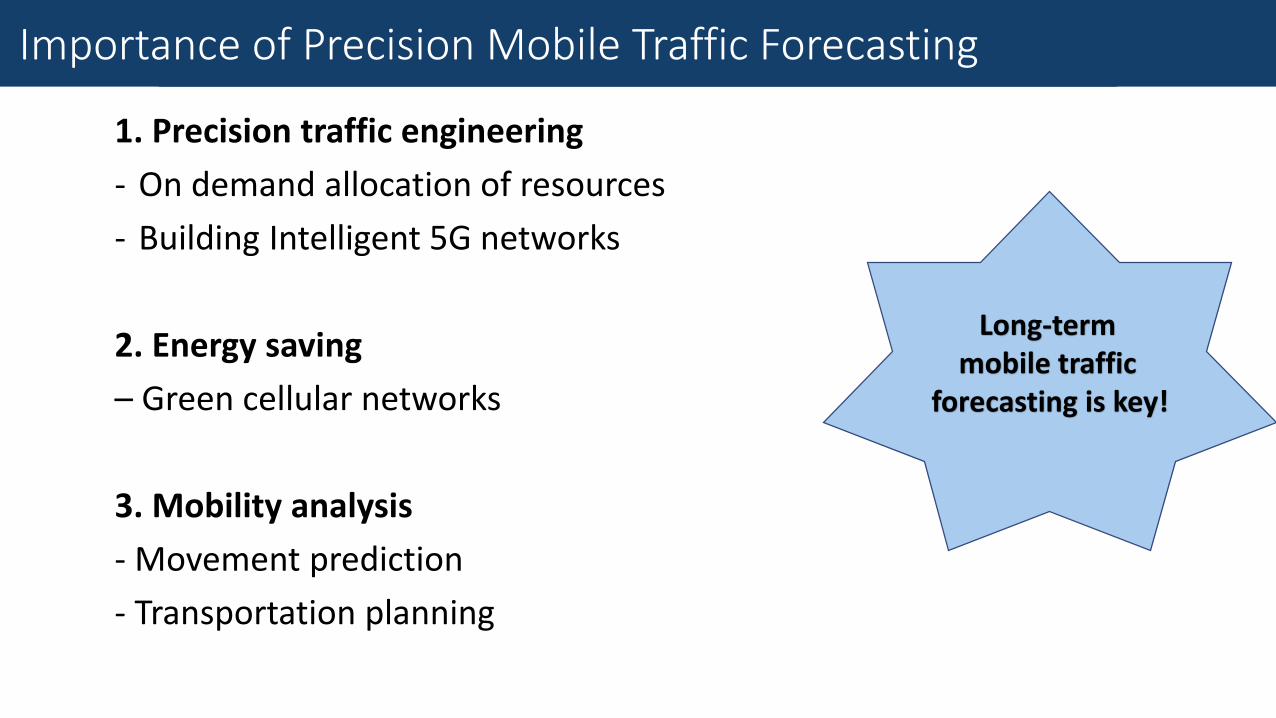
1. Precision traffic engineering
- On demand allocation of resources
- Building Intelligent 5G networks
2. Energy saving
– Green cellular networks
3. Mobility analysis
- Movement prediction
- Transportation planning
Importance of Precision Mobile Traffic Forecasting
Long-term mobile traffic
forecasting is key!
Fine-Grained Traffic Measurement
1. Rely on dedicated infrastructure
•Packet Gateway (PGW) or Radio Network Controller (RNC) probes
•Data storage
Continuous measurements are expensive
Fine-Grained Traffic Measurement
1. Rely on dedicated infrastructure
•Packet Gateway (PGW) or Radio Network Controller (RNC) probes
•Data storage
2. Data post-processing overheads
•Call detail record reports transfer
•Spatial aggregation
Continuous measurements are expensive
Fine-Grained Traffic Measurement
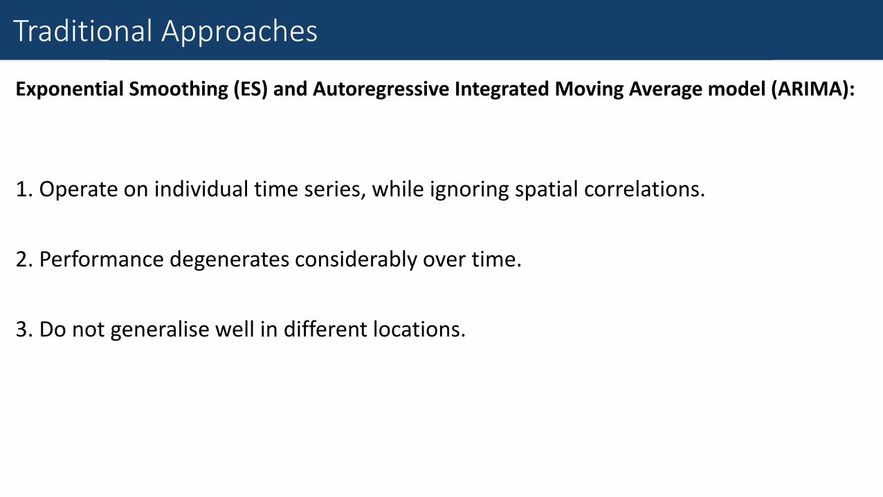
Exponential Smoothing (ES) and Autoregressive Integrated Moving Average model (ARIMA):
1. Operate on individual time series, while ignoring spatial correlations.
2. Performance degenerates considerably over time.
3. Do not generalise well in different locations.
Traditional Approaches
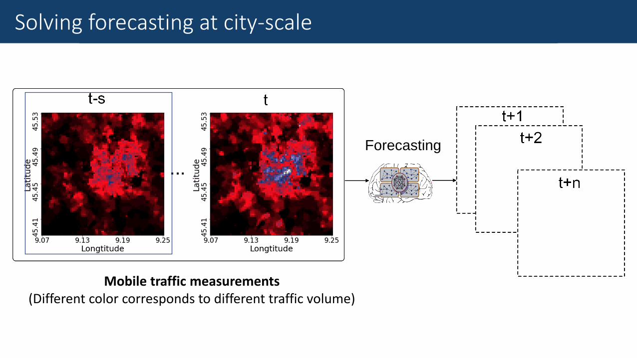
The Goal of Mobile Traffic AnalysisSolving forecasting at city-scale
Mobile traffic measurements(Different color corresponds to different traffic volume)
Forecasting
Fine-Grained Traffic Measurement
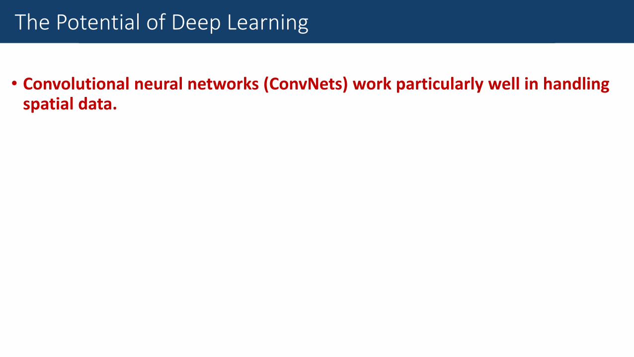
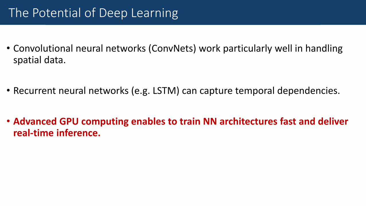
• Convolutional neural networks (ConvNets) work particularly well in handling spatial data.
The Potential of Deep Learning
Fine-Grained Traffic Measurement
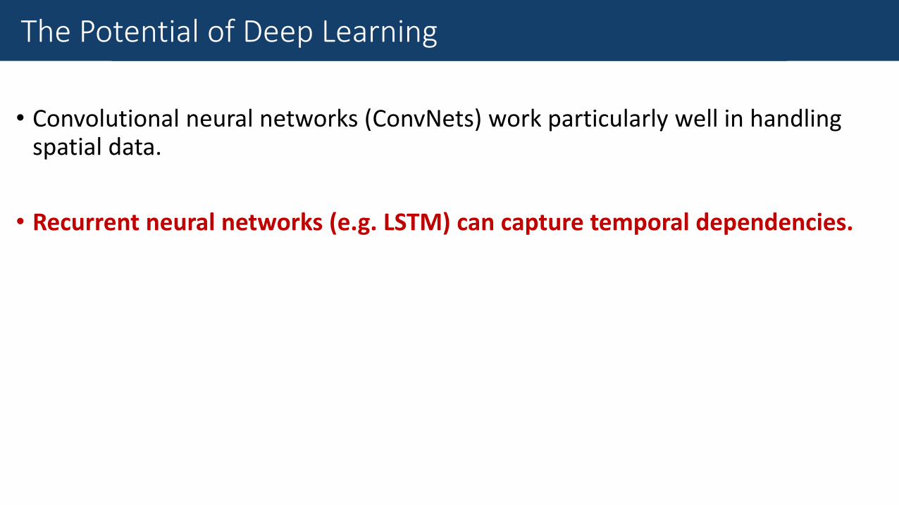
• Convolutional neural networks (ConvNets) work particularly well in handling spatial data.
• Recurrent neural networks (e.g. LSTM) can capture temporal dependencies.
The Potential of Deep Learning
Fine-Grained Traffic Measurement
• Convolutional neural networks (ConvNets) work particularly well in handling spatial data.
• Recurrent neural networks (e.g. LSTM) can capture temporal dependencies.
• Advanced GPU computing enables to train NN architectures fast and deliver real-time inference.
The Potential of Deep Learning
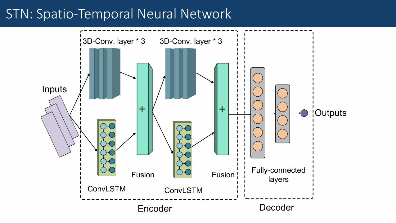
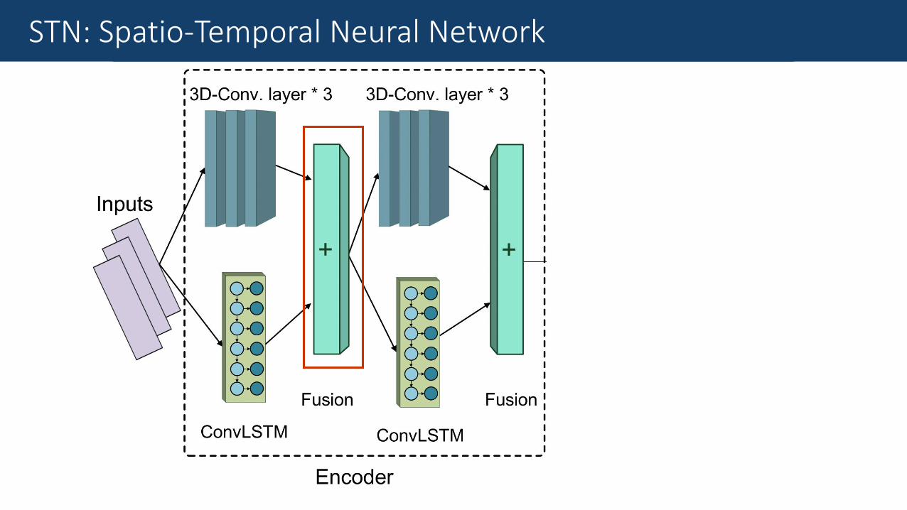
Fine-Grained Traffic MeasurementSTN: Spatio-Temporal Neural Network
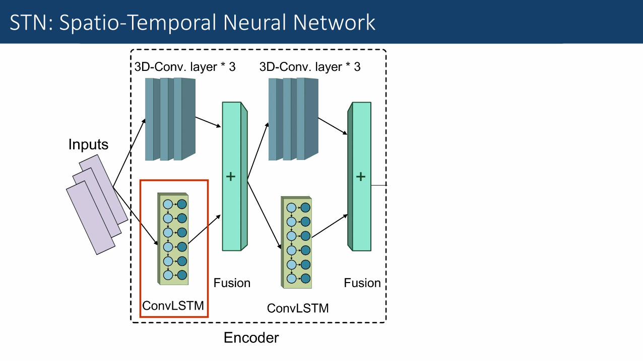
Fine-Grained Traffic MeasurementSTN: Spatio-Temporal Neural Network
Fine-Grained Traffic MeasurementConvLSTM
Convolutional Long Short-Term Memory (ConvLSTM)
•Advanced version of LSTM.
•Replaces inner dense connections with convolution operations.
•Works remarkably well in modelling spatio-temporal data.
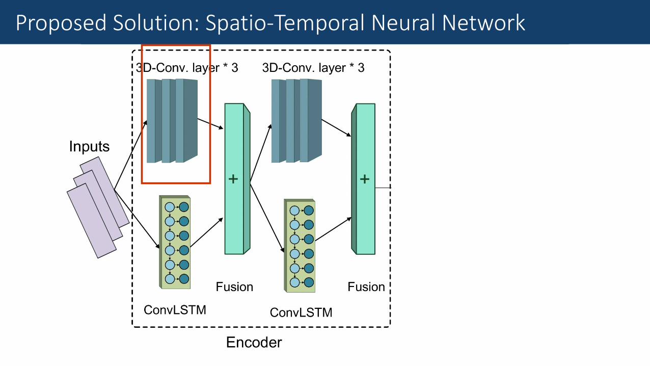
Fine-Grained Traffic MeasurementProposed Solution: Spatio-Temporal Neural Network
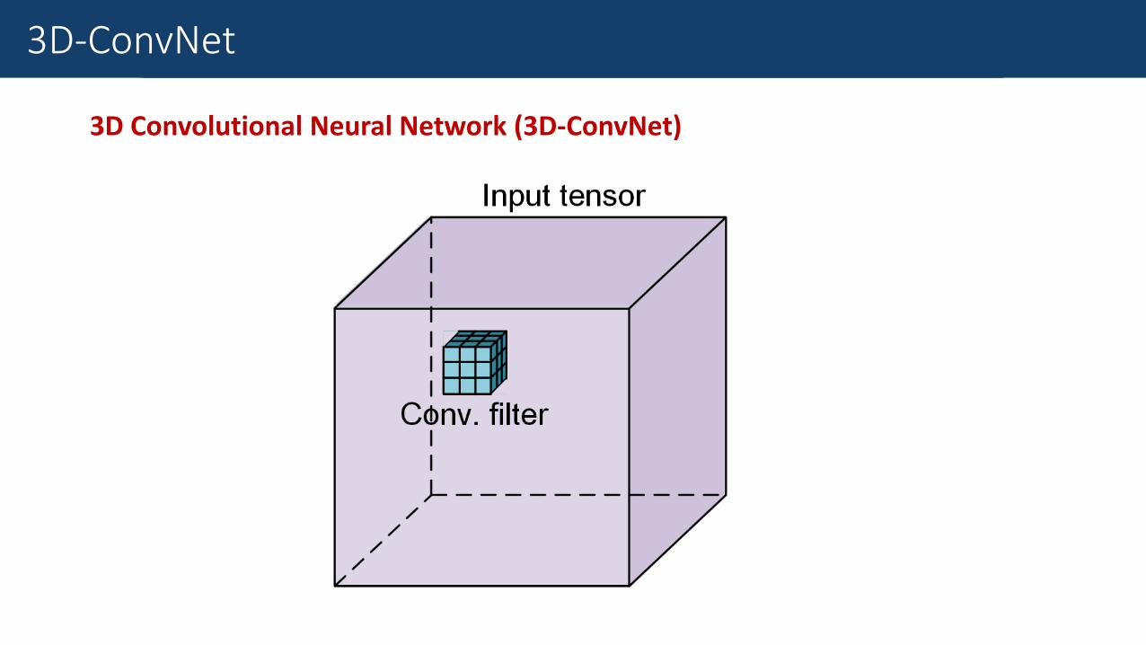
Fine-Grained Traffic Measurement3D-ConvNet
3D Convolutional Neural Network (3D-ConvNet)
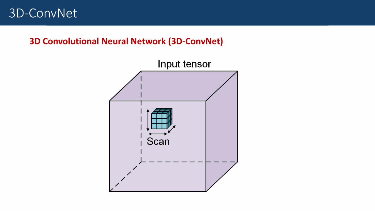
Fine-Grained Traffic Measurement3D-ConvNet
3D Convolutional Neural Network (3D-ConvNet)
Fine-Grained Traffic MeasurementSTN: Spatio-Temporal Neural Network
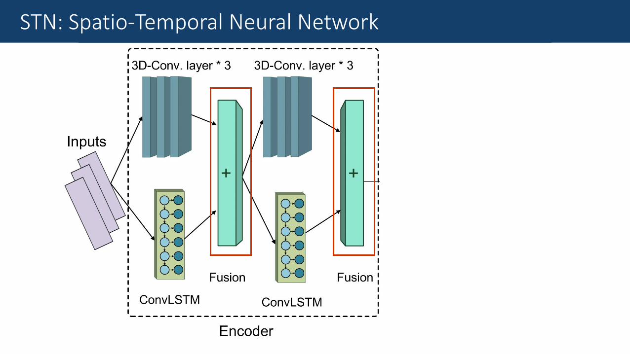
Fine-Grained Traffic MeasurementSTN: Spatio-Temporal Neural Network

Fine-Grained Traffic MeasurementSTN: Spatio-Temporal Neural Network
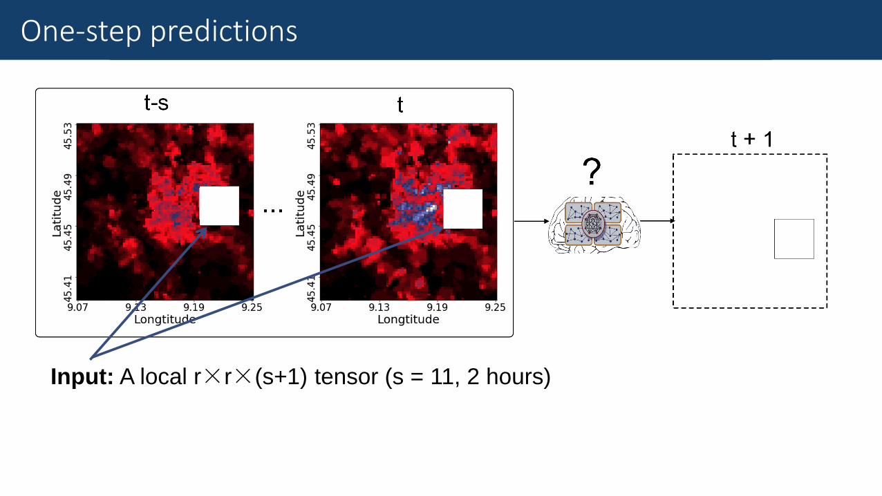
Fine-Grained Traffic MeasurementOne-step predictions
Input: A local r×r×(s+1) tensor (s = 11, 2 hours)
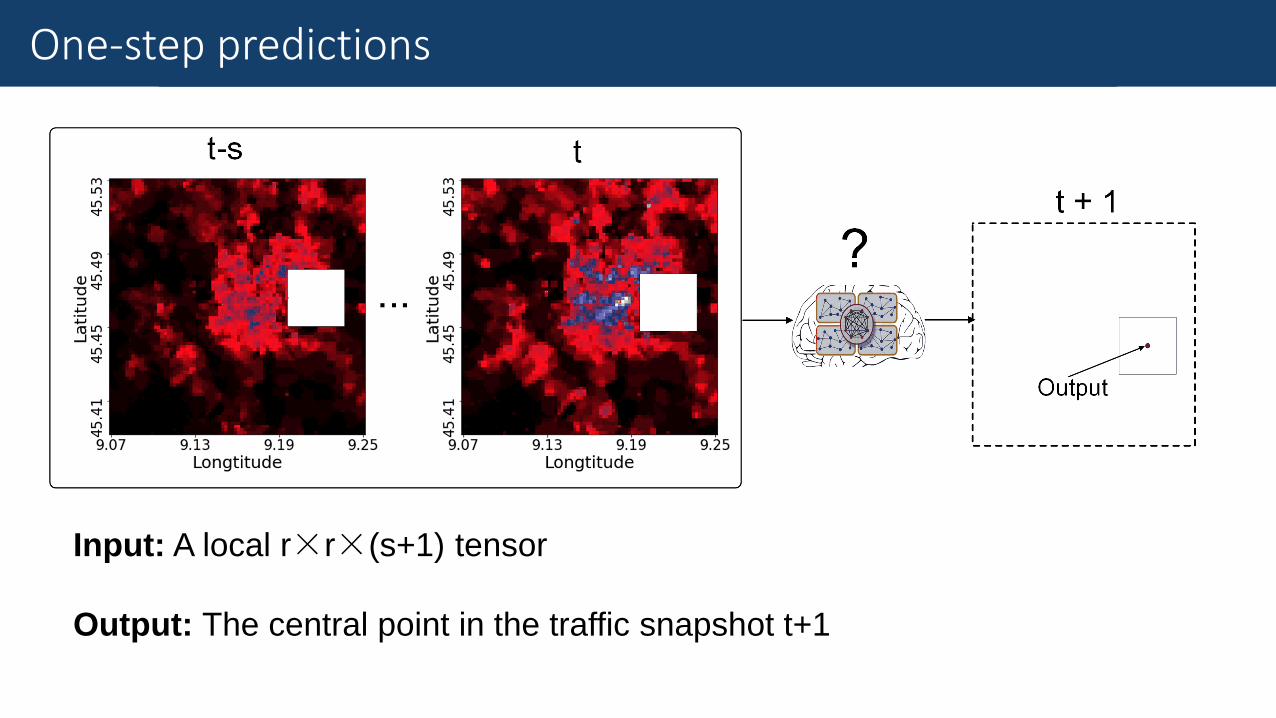
Fine-Grained Traffic MeasurementOne-step predictions
Input: A local r×r×(s+1) tensor
Output: The central point in the traffic snapshot t+1
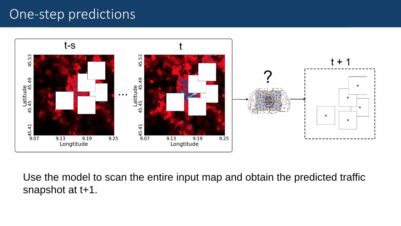
Fine-Grained Traffic MeasurementOne-step predictions
Use the model to scan the entire input map and obtain the predicted traffic
snapshot at t+1.

Fine-Grained Traffic MeasurementOne-step predictions
• The traffic consumption at a certain location largely depends on that in its
neighouring cells.
Fine-Grained Traffic Measurement
Feeding the model with previous forecasts: Error accumulates.
Extending to Long-Term Forecasting
Fine-Grained Traffic Measurement
Feeding the model with previous forecasts: Error accumulates.
Extending to Long-Term Forecasting
Fine-Grained Traffic Measurement
Feeding the model with previous forecasts: Error accumulates.
Extending to Long-Term Forecasting
Ideal
Fine-Grained Traffic Measurement
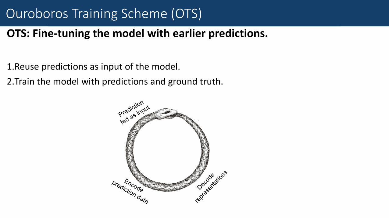
OTS: Fine-tuning the model with earlier predictions.
Fine-Tune with Earlier Prediction
Ouroboros Training Scheme (OTS)
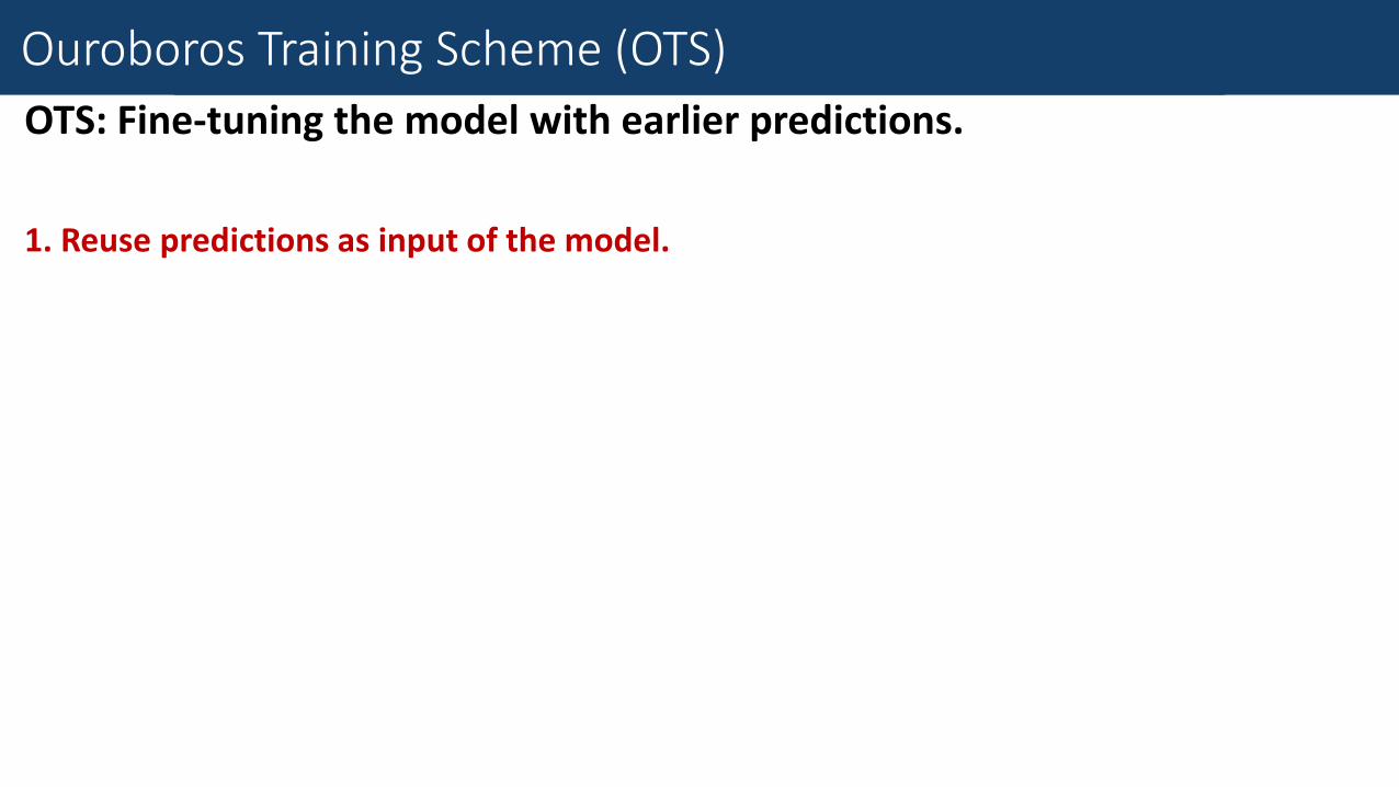
Fine-Grained Traffic Measurement
OTS: Fine-tuning the model with earlier predictions.
1. Reuse predictions as input of the model.
Fine-Tune with Earlier Prediction
Ouroboros Training Scheme (OTS)
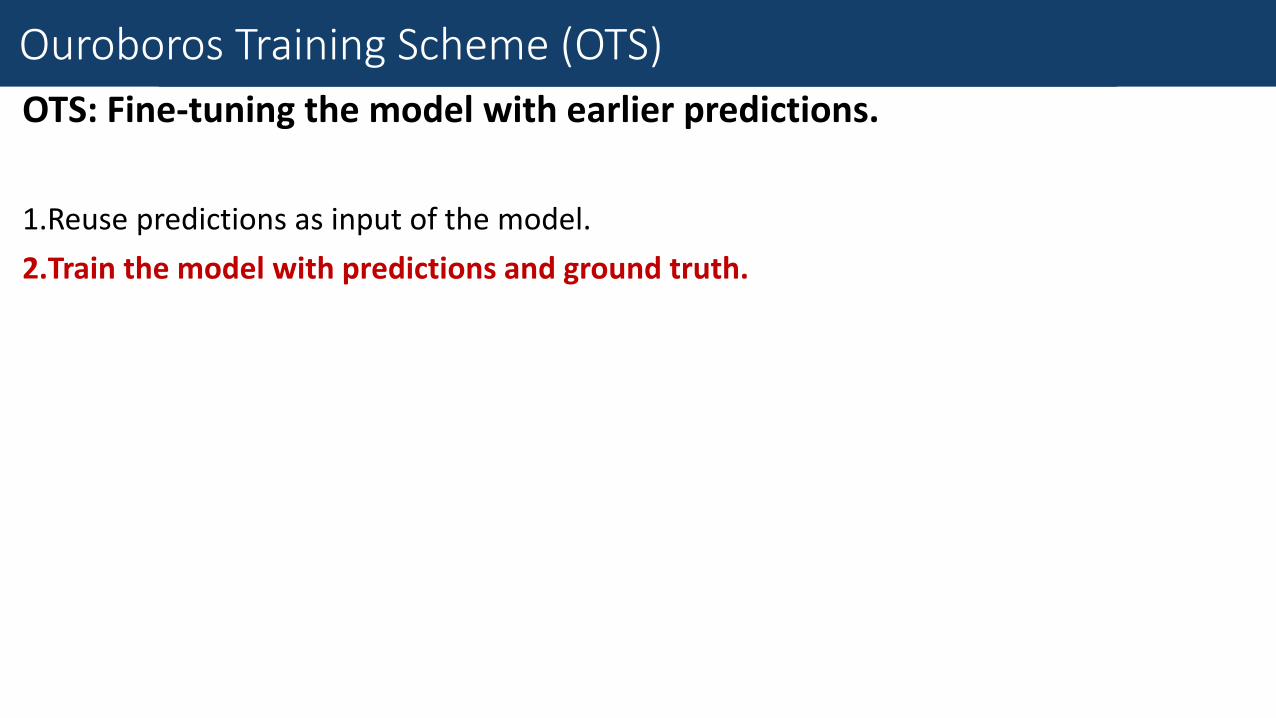
Fine-Grained Traffic Measurement
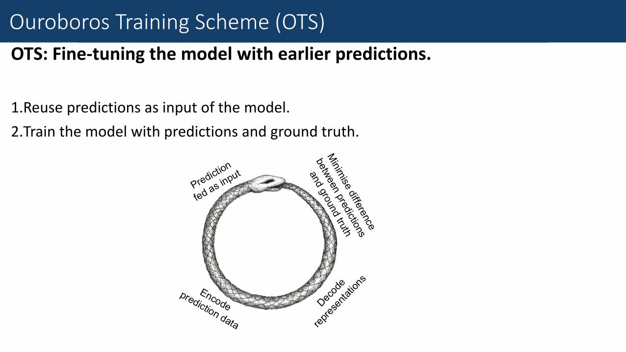
OTS: Fine-tuning the model with earlier predictions.
1.Reuse predictions as input of the model.
2.Train the model with predictions and ground truth.
Fine-Tune with Earlier Prediction
Ouroboros Training Scheme (OTS)
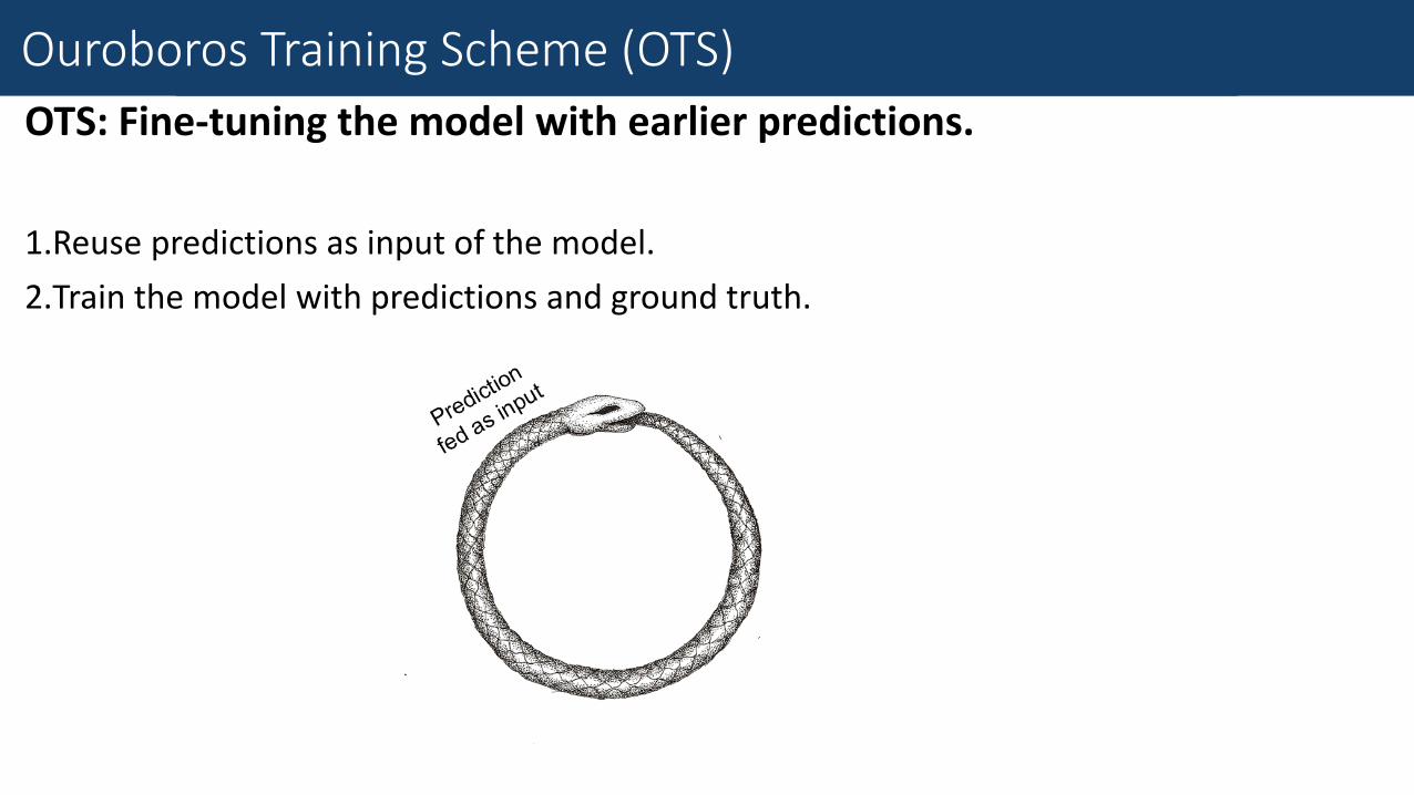
Fine-Grained Traffic Measurement
OTS: Fine-tuning the model with earlier predictions.
1.Reuse predictions as input of the model.
2.Train the model with predictions and ground truth.
Fine-Tune with Earlier Prediction
Ouroboros Training Scheme (OTS)
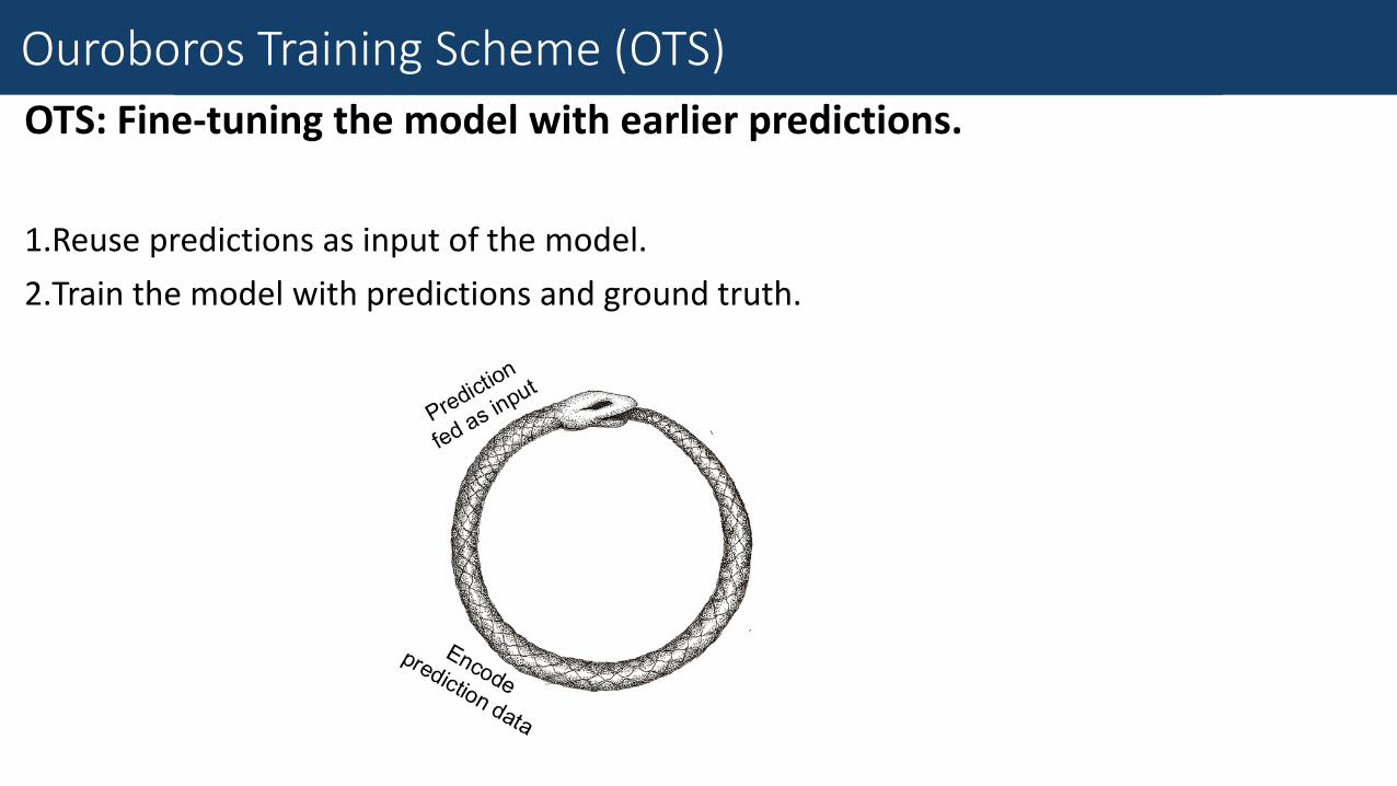
Fine-Grained Traffic Measurement
OTS: Fine-tuning the model with earlier predictions.
1.Reuse predictions as input of the model.
2.Train the model with predictions and ground truth.
Fine-Tune with Earlier Prediction
Ouroboros Training Scheme (OTS)
Fine-Grained Traffic Measurement
OTS: Fine-tuning the model with earlier predictions.
1.Reuse predictions as input of the model.
2.Train the model with predictions and ground truth.
Fine-Tune with Earlier Prediction
Ouroboros Training Scheme (OTS)
Fine-Grained Traffic Measurement
OTS: Fine-tuning the model with earlier predictions.
1.Reuse predictions as input of the model.
2.Train the model with predictions and ground truth.
Fine-Tune with Earlier Prediction
Ouroboros Training Scheme (OTS)
Fine-Grained Traffic Measurement
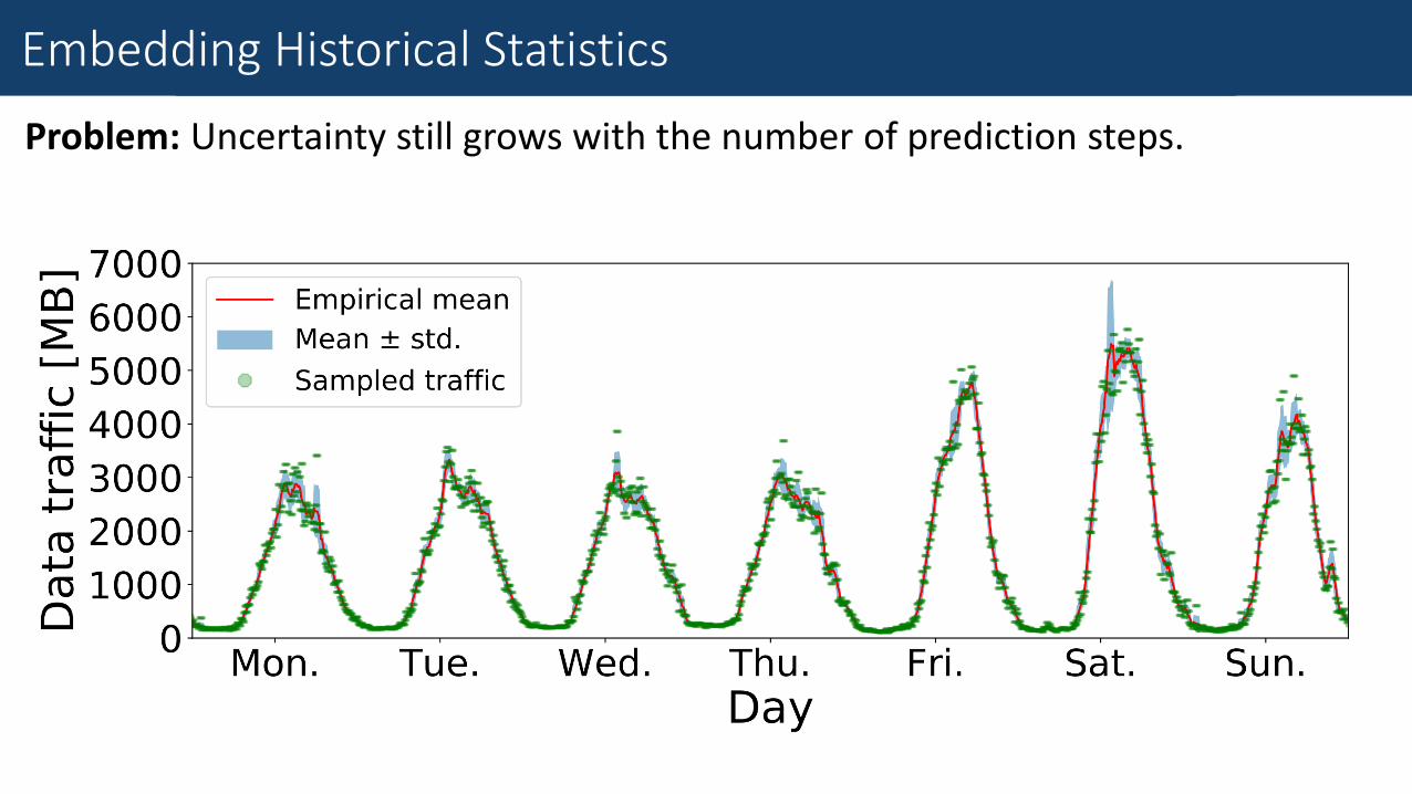
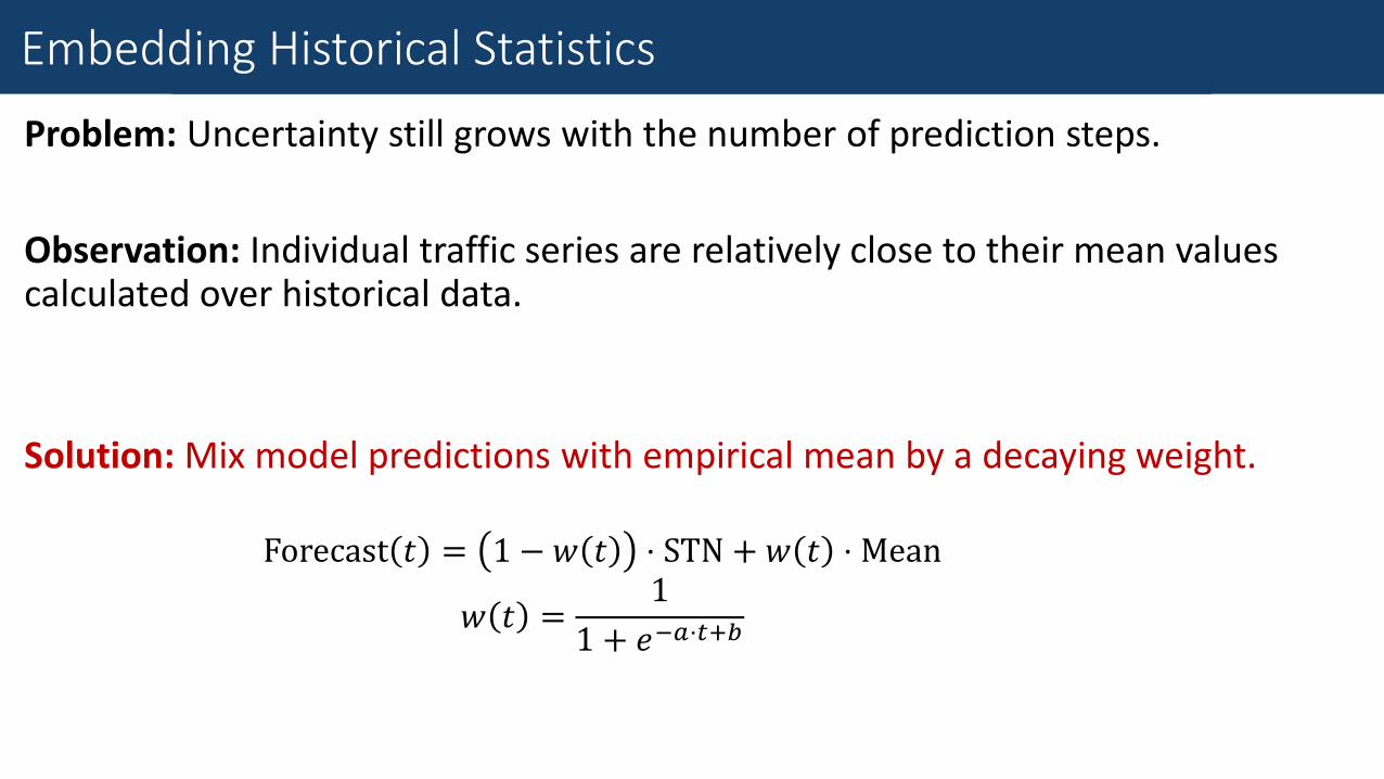
Problem: Uncertainty still grows with the number of prediction steps.
Embedding Historical Statistics
Fine-Grained Traffic Measurement
Problem: Uncertainty still grows with the number of prediction steps.
Observation: Individual traffic series are relatively close to their mean values calculated over historical data.
Embedding Historical Statistics
Fine-Grained Traffic Measurement
Problem: Uncertainty still grows with the number of prediction steps.
Embedding Historical Statistics
Fine-Grained Traffic Measurement
Problem: Uncertainty still grows with the number of prediction steps.
Observation: Individual traffic series are relatively close to their mean values calculated over historical data.
Solution: Mix model predictions with empirical mean by a decaying weight.
Embedding Historical Statistics
Forecast 𝑡 = 1 − 𝑤 𝑡 ⋅ STN + 𝑤 𝑡 ⋅ Mean
𝑤 𝑡 =1
1 + 𝑒−𝑎⋅𝑡+𝑏
Fine-Grained Traffic Measurement
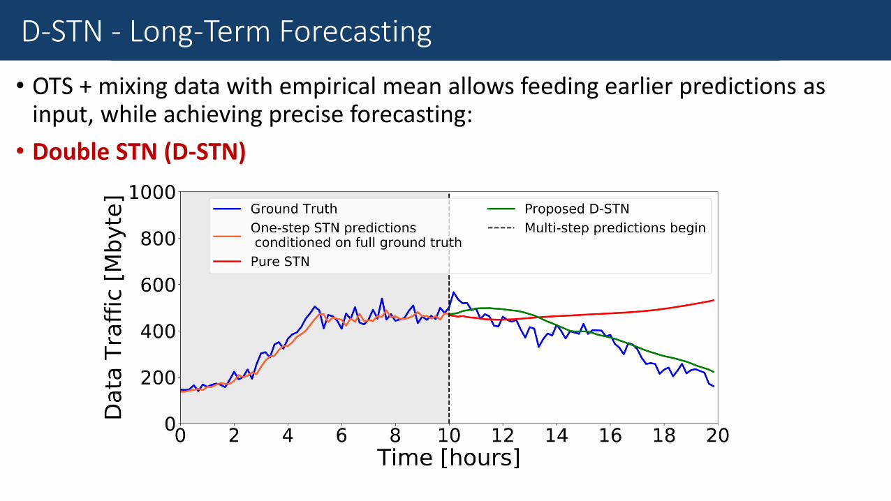
• OTS + mixing data with empirical mean allows feeding earlier predictions as input, while achieving precise forecasting:
• Double STN (D-STN)
D-STN - Long-Term Forecasting

Dataset
• Telecom Italia's Big Data Challenge
Dataset
Dataset
• Telecom Italia's Big Data Challenge
• Measurements of mobile traffic volume between 1 Nov 2013 and 1 Jan 2014 in the city of Milan and province of Trentino.
Dataset
Dataset
• Telecom Italia's Big Data Challenge
• Measurements of mobile traffic volume between 1 Nov 2013 and 1 Jan 2014 in the city of Milan and province of Trentino.
• Aggregated every 10 minutes.
Dataset
Dataset
• Telecom Italia's Big Data Challenge
• Measurements of mobile traffic volume between 1 Nov 2013 and 1 Jan 2014 in the city of Milan and province of Trentino.
• Aggregated every 10 minutes.
• Partitioned in 100×100 grids for Milan and 117×98 grids for Trentino.
Dataset
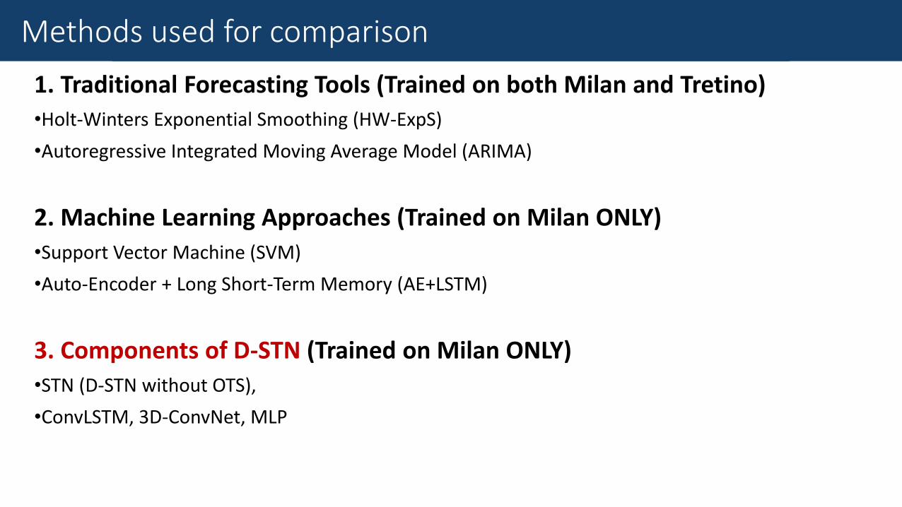
Methods for Comparison
1. Traditional Forecasting Tools (Trained on both Milan and Trentino)
•Holt-Winters Exponential Smoothing (HW-ExpS)
•Autoregressive Integrated Moving Average Model (ARIMA)
Methods used for comparison
Methods for Comparison
1. Traditional Forecasting Tools (Trained on both Milan and Tretino)
•Holt-Winters Exponential Smoothing (HW-ExpS)
•Autoregressive Integrated Moving Average Model (ARIMA)
2. Machine Learning Approaches (Trained on Milan ONLY)
•Support Vector Machine (SVM)
•Auto-Encoder + Long Short-Term Memory (AE+LSTM)
Methods used for comparison
Methods for Comparison
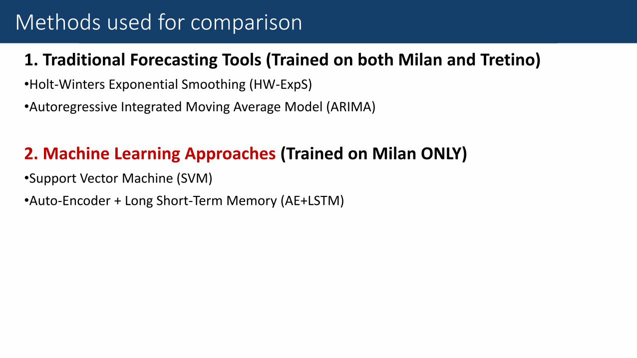
1. Traditional Forecasting Tools (Trained on both Milan and Tretino)
•Holt-Winters Exponential Smoothing (HW-ExpS)
•Autoregressive Integrated Moving Average Model (ARIMA)
2. Machine Learning Approaches (Trained on Milan ONLY)
•Support Vector Machine (SVM)
•Auto-Encoder + Long Short-Term Memory (AE+LSTM)
3. Components of D-STN (Trained on Milan ONLY)
•STN (D-STN without OTS),
•ConvLSTM, 3D-ConvNet, MLP
Methods used for comparison
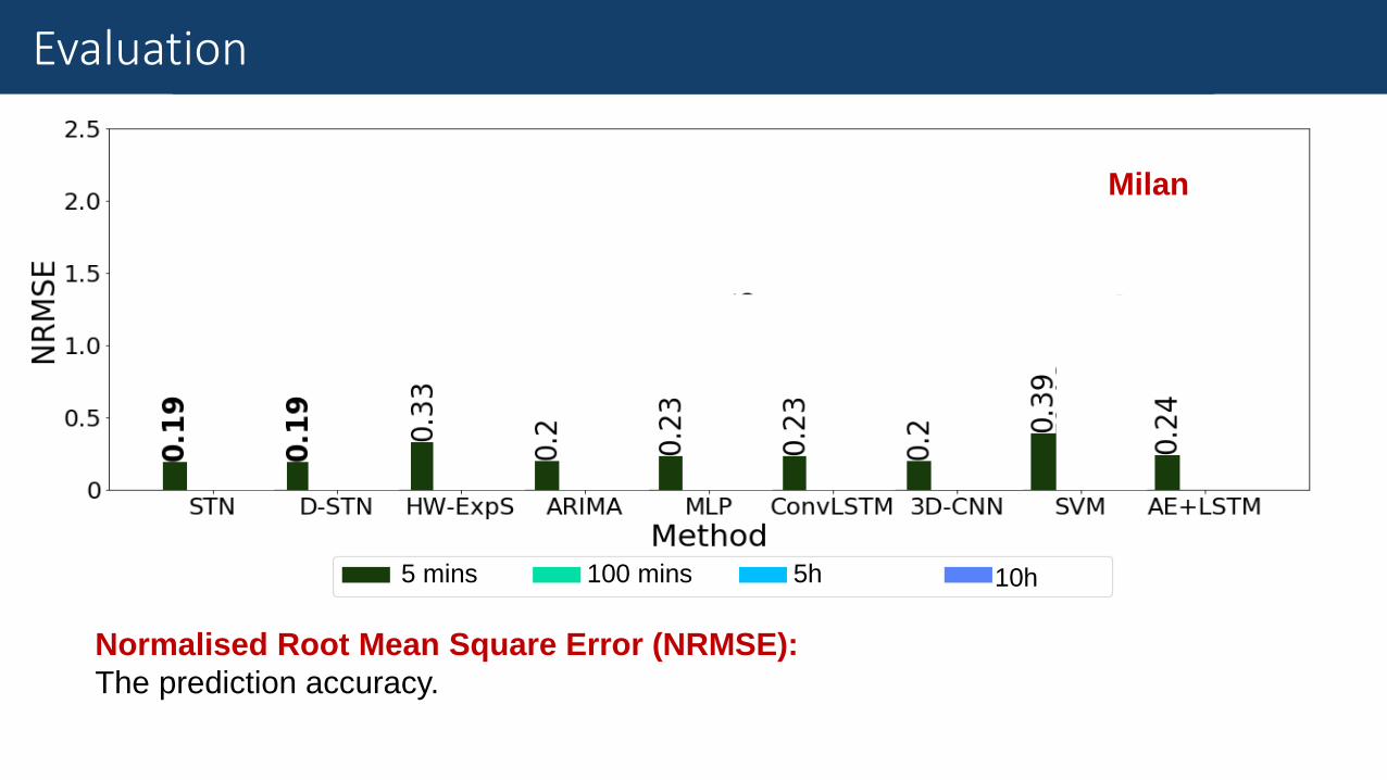
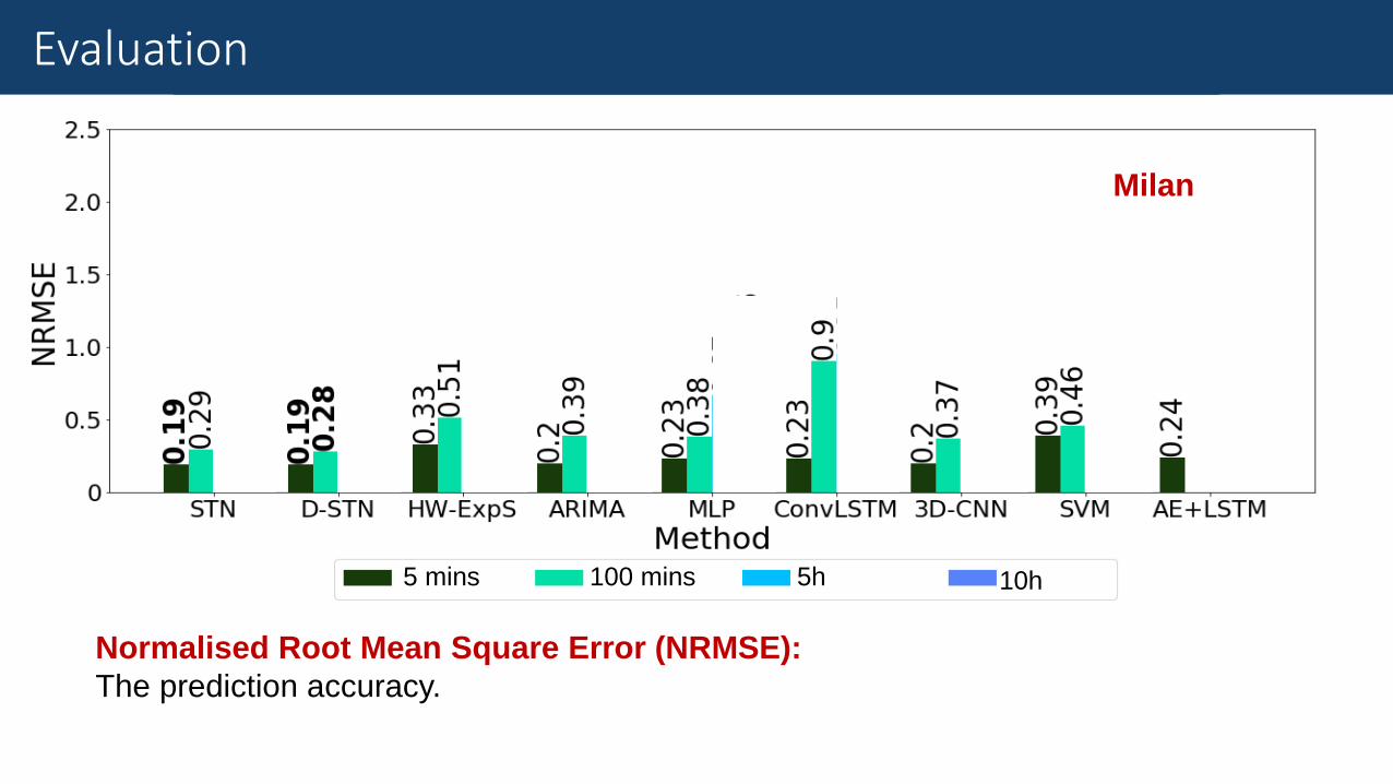
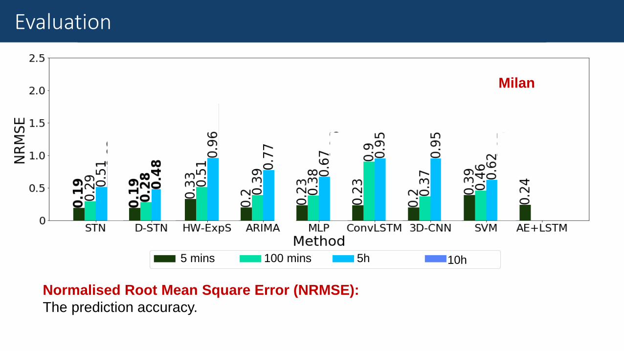
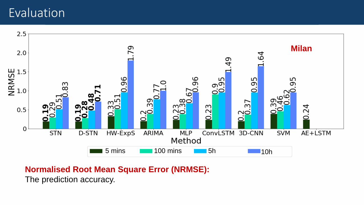
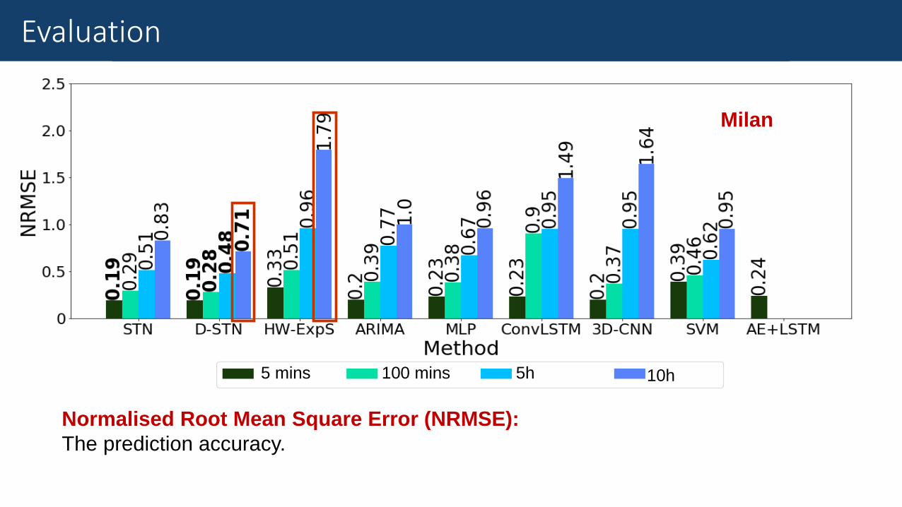
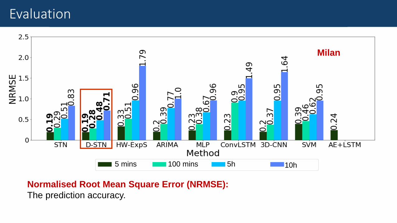
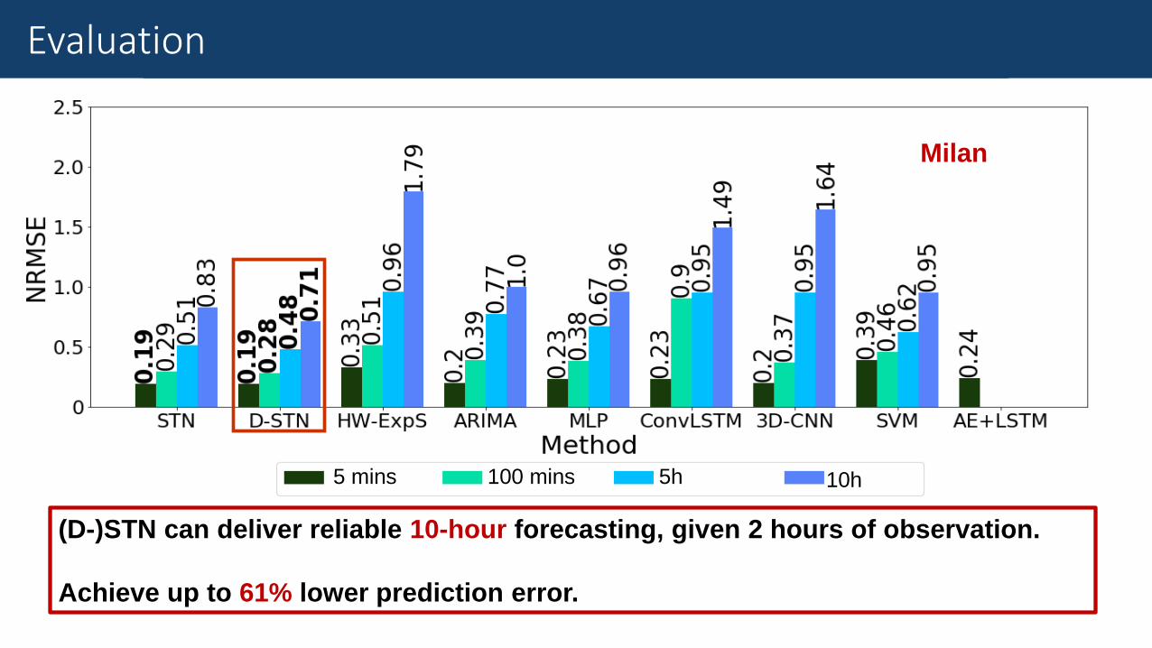
Results
Normalised Root Mean Square Error (NRMSE):
The prediction accuracy.
Evaluation
Milan
5 mins 100 mins 5h 10h
Results
Normalised Root Mean Square Error (NRMSE):
The prediction accuracy.
Evaluation
Milan
5 mins 100 mins 5h 10h
Results
Normalised Root Mean Square Error (NRMSE):
The prediction accuracy.
Evaluation
Milan
5 mins 100 mins 5h 10h
Results
Normalised Root Mean Square Error (NRMSE):
The prediction accuracy.
Evaluation
Milan
5 mins 100 mins 5h 10h
Results
Normalised Root Mean Square Error (NRMSE):
The prediction accuracy.
Evaluation
Milan
5 mins 100 mins 5h 10h
Results
Normalised Root Mean Square Error (NRMSE):
The prediction accuracy.
Evaluation
Milan
5 mins 100 mins 5h 10h
ResultsEvaluation
Milan
5 mins 100 mins 5h 10h
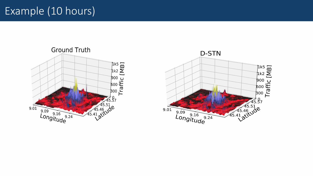
(D-)STN can deliver reliable 10-hour forecasting, given 2 hours of observation.
Achieve up to 61% lower prediction error.
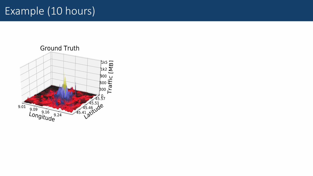
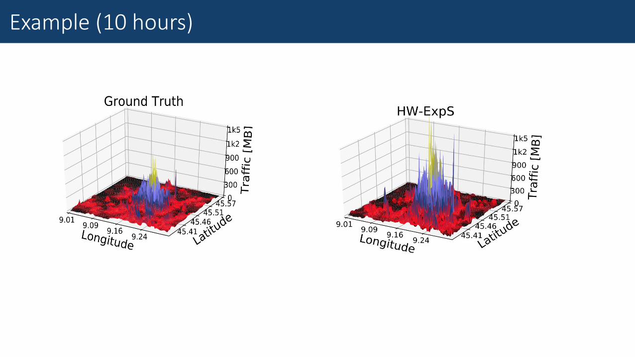
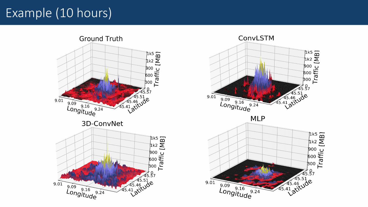
Example (10 hours)
Example (10 hours)
Example (10 hours)
Example (10 hours)
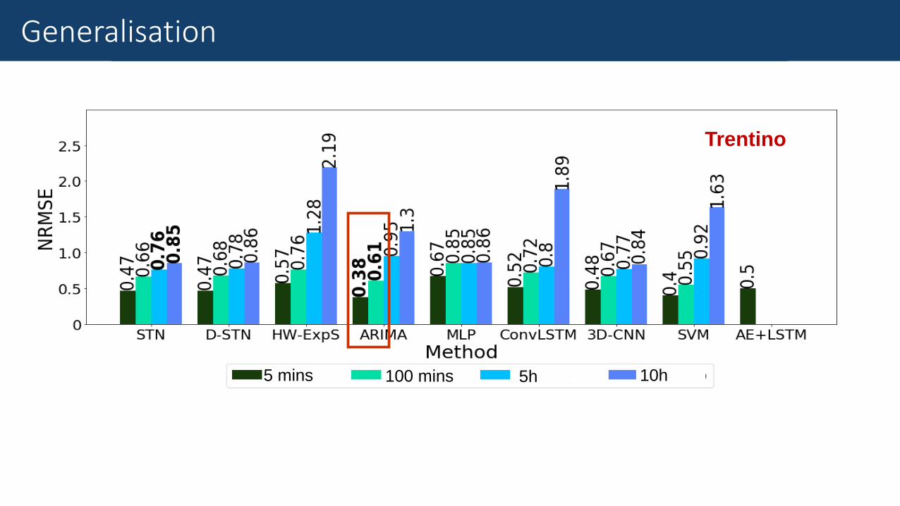
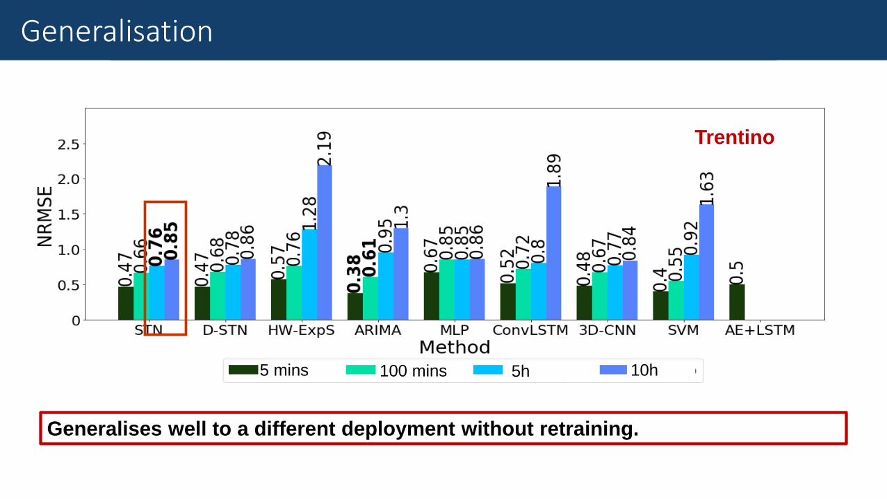
ResultsGeneralisation
Trentino
5 mins 100 mins 5h 10h
ResultsGeneralisation
Trentino
5 mins 100 mins 5h 10h
Generalises well to a different deployment without retraining.
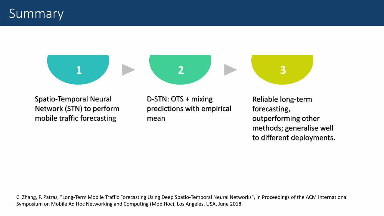
Spatio-Temporal Neural Network (STN) to perform mobile traffic forecasting
1
D-STN: OTS + mixing predictions with empirical mean
2
Reliable long-term forecasting, outperforming other methods; generalise well to different deployments.
3
Summary
C. Zhang, P. Patras, "Long-Term Mobile Traffic Forecasting Using Deep Spatio-Temporal Neural Networks", in Proceedings of the ACM International Symposium on Mobile Ad Hoc Networking and Computing (MobiHoc), Los Angeles, USA, June 2018.

Maximising the utility of virtualised backhauls
• 5G networks need to accommodate services with distinct performance requirements• Bandwidth: UHD video streaming and AR/VR
• Delay: Autonomous vehicles and remote medical care
• Network slicing• Partitioning physical infrastructure into logically isolated networks
• Network densification• High speed wireless backhauling tangible (mm-wave, free space optics, etc.)
Increasingly diverse services
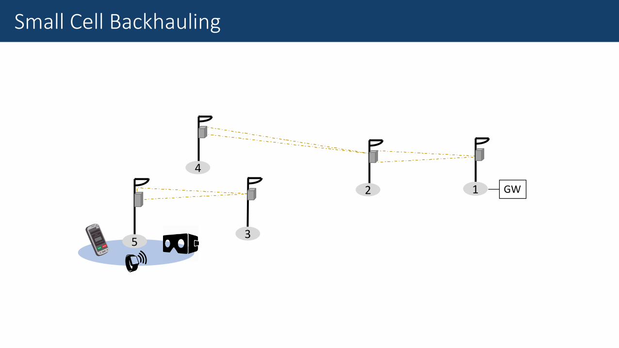
1 GW2
3
4
5
Small Cell Backhauling
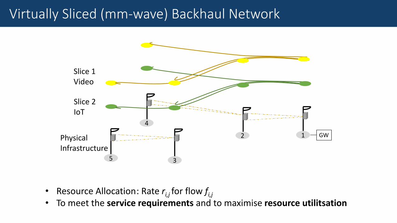
Slice2IoT
Slice1Video
1 GWPhysicalInfrastructure
2
3
4
5
• Resource Allocation• To meet the service requirements and to maximise resource utilitsation
: Rate ri,j for flow fi,j
Virtually Sliced (mm-wave) Backhaul Network
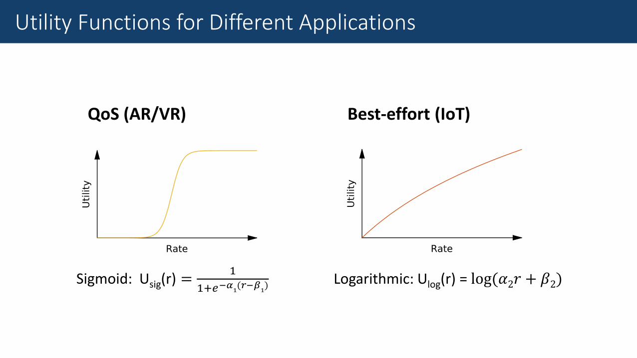
Best-effort (IoT)
Logarithmic: Ulog(r) = log(𝛼2𝑟 + 𝛽2)
QoS (AR/VR)
Sigmoid: Usig(r) =1
1+𝑒−𝛼1(𝑟−𝛽
1)
Utility Functions for Different Applications
Utility Functions for Different Applications
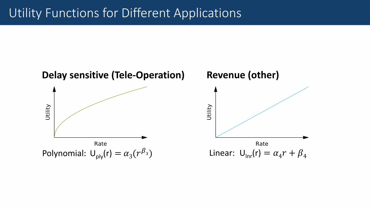
Delay sensitive (Tele-Operation)
Polynomial: Uply(r) = 𝛼3(𝑟𝛽3)
Revenue (other)
Linear: Ulnr(r) = 𝛼4𝑟 + 𝛽4
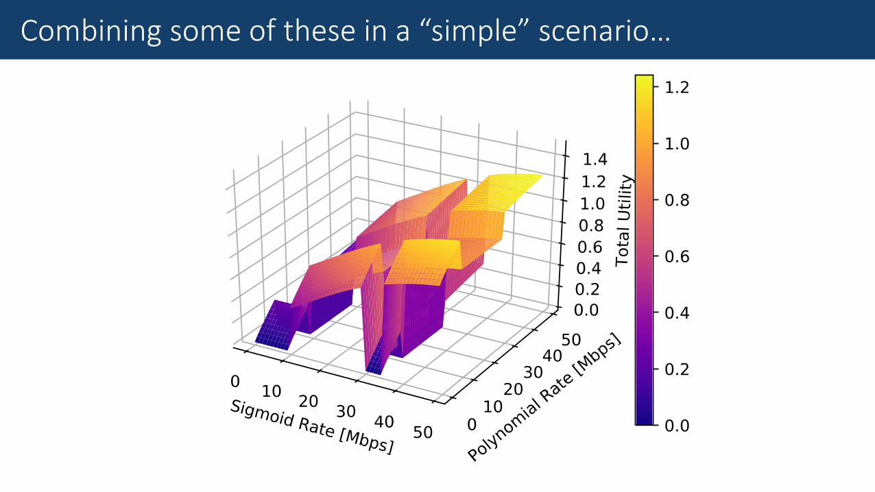
Combining some of these in a “simple” scenario…
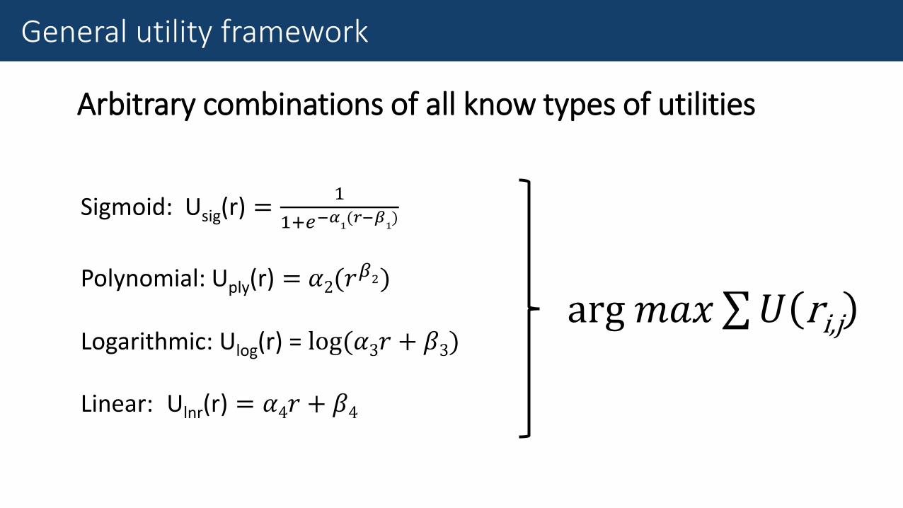
Arbitrary combinations of all know types of utilities
Sigmoid: Usig(r) =1
1+𝑒−𝛼1(𝑟−𝛽
1)
Polynomial: Uply(r) = 𝛼2(𝑟𝛽2)
Logarithmic: Ulog(r) = log(𝛼3𝑟 + 𝛽3)
Linear: Ulnr(r) = 𝛼4𝑟 + 𝛽4
arg 𝑚𝑎𝑥 σ𝑈 ri,j
General utility framework
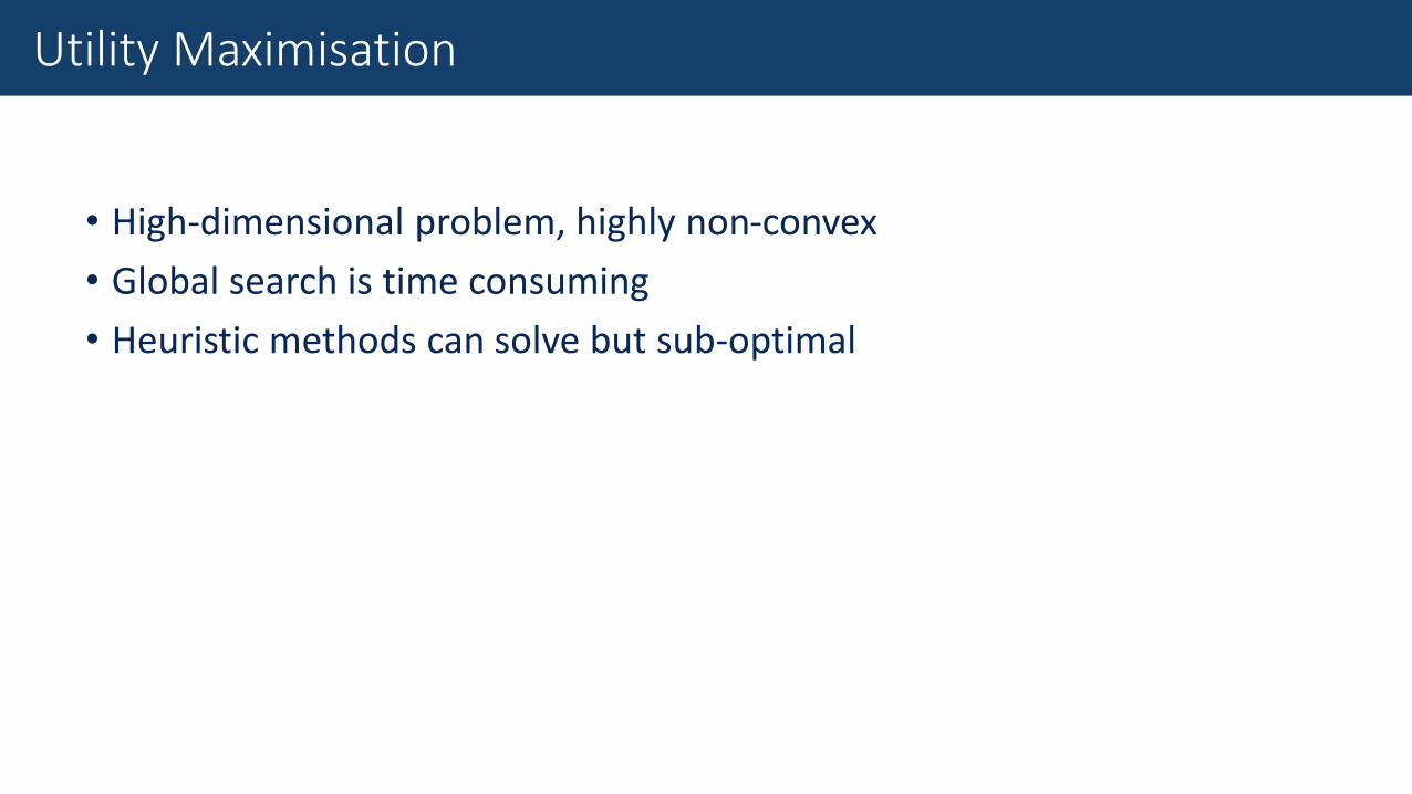
• High-dimensional problem, highly non-convex
• Global search is time consuming
• Heuristic method can solve but sub-optimal
• High-dimensional problem, highly non-convex
• Global search is time consuming
• Heuristic methods can solve but sub-optimal
Utility Maximisation
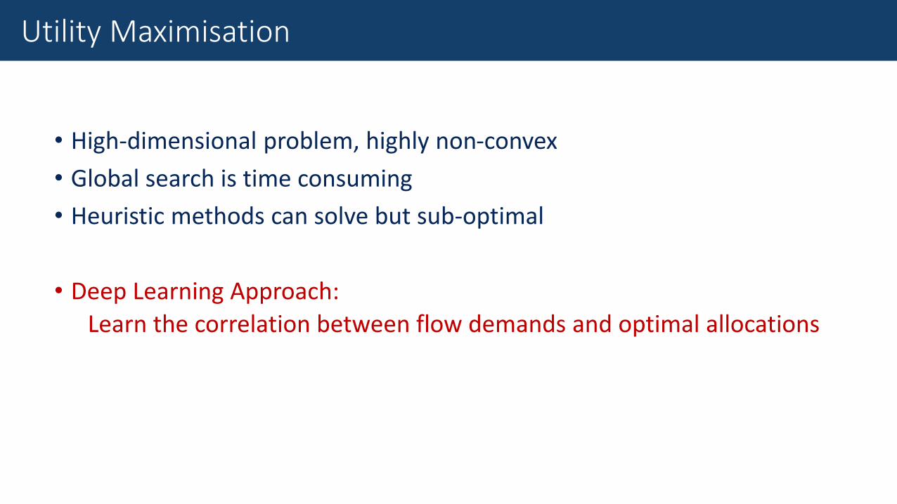
• High-dimensional problem, highly non-convex
• Global search is time consuming
• Heuristic method can solve but sub-optimal
• Deep Learning Approach:
Learn the correlation between flow demands and optimal allocations
• High-dimensional problem, highly non-convex
• Global search is time consuming
• Heuristic methods can solve but sub-optimal
Utility Maximisation
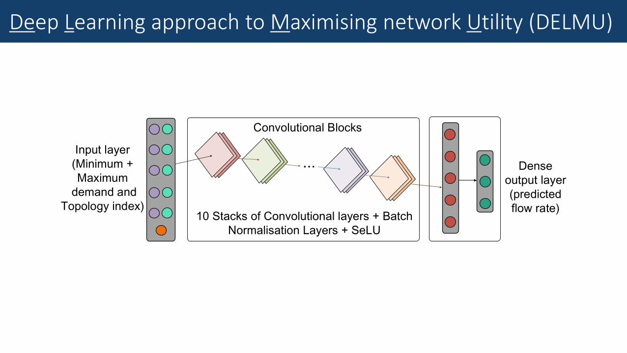
Deep Learning approach to Maximising network Utility (DELMU)
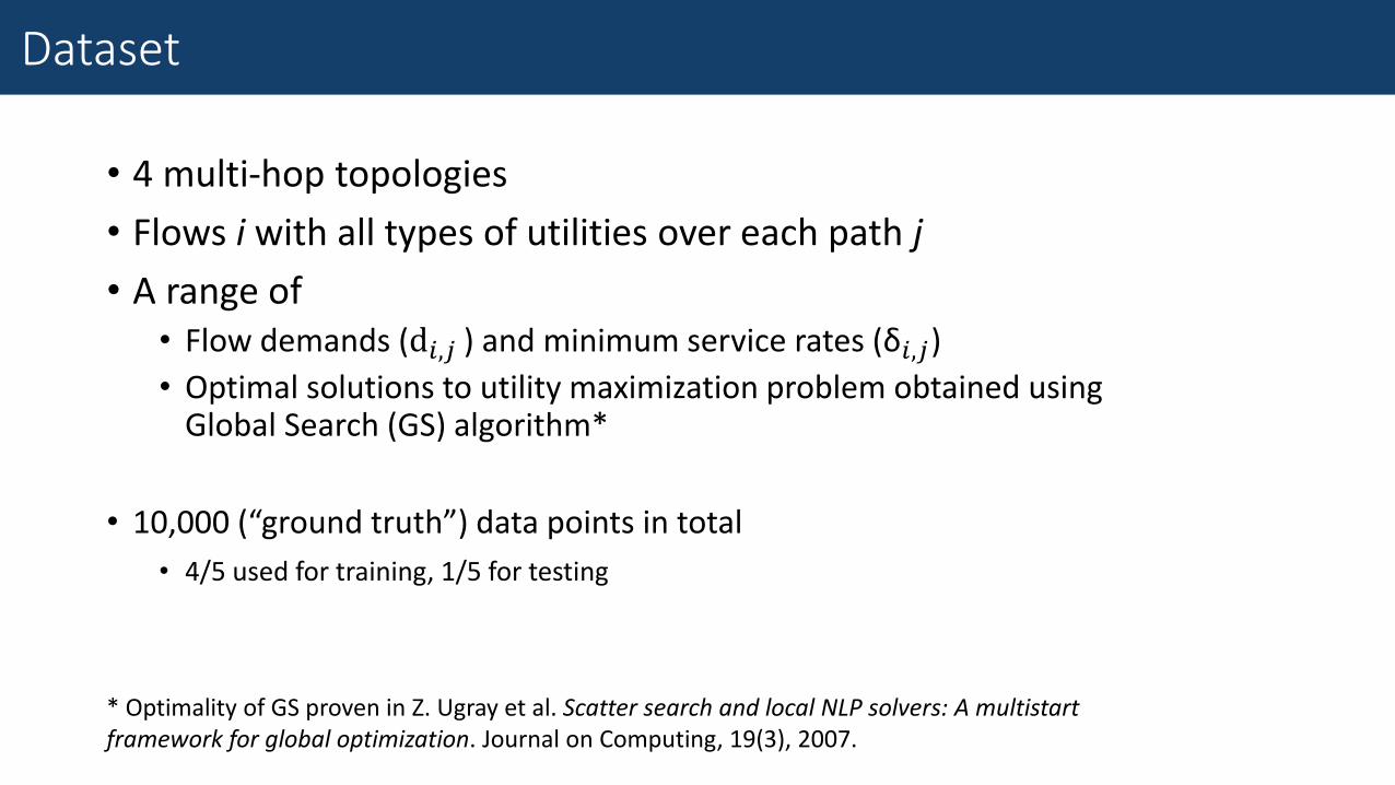
• 4 multi-hop topologies
• Flows i with all types of utilities over each path j
• A range of • Flow demands (d𝑖,𝑗 ) and minimum service rates (δ𝑖,𝑗)
• Optimal solutions to utility maximization problem obtained using Global Search (GS) algorithm*
• 10,000 (“ground truth”) data points in total
• 4/5 used for training, 1/5 for testing
* Optimality of GS proven in Z. Ugray et al. Scatter search and local NLP solvers: A multistartframework for global optimization. Journal on Computing, 19(3), 2007.
Dataset
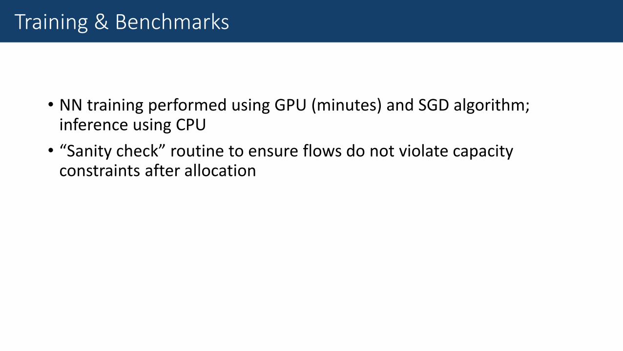
• NN training performed using GPU (minutes) and SGD algorithm; inference using CPU
• “Sanity check” routine to ensure flows do not violate capacity constraints after allocation
Training & Benchmarks
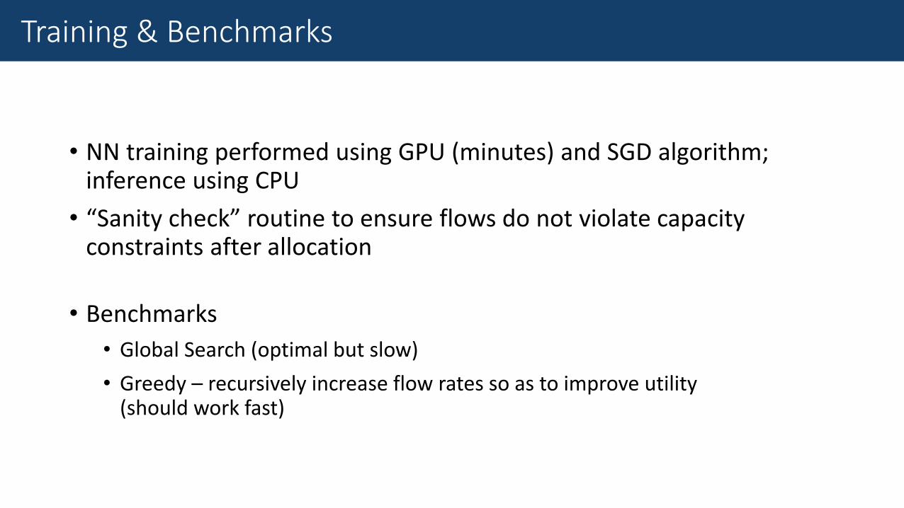
• NN training performed using GPU (minutes) and SGD algorithm; inference using CPU
• “Sanity check” routine to ensure flows do not violate capacity constraints after allocation
• Benchmarks
• Global Search (optimal but slow)
• Greedy – recursively increase flow rates so as to improve utility (should work fast)
Training & Benchmarks
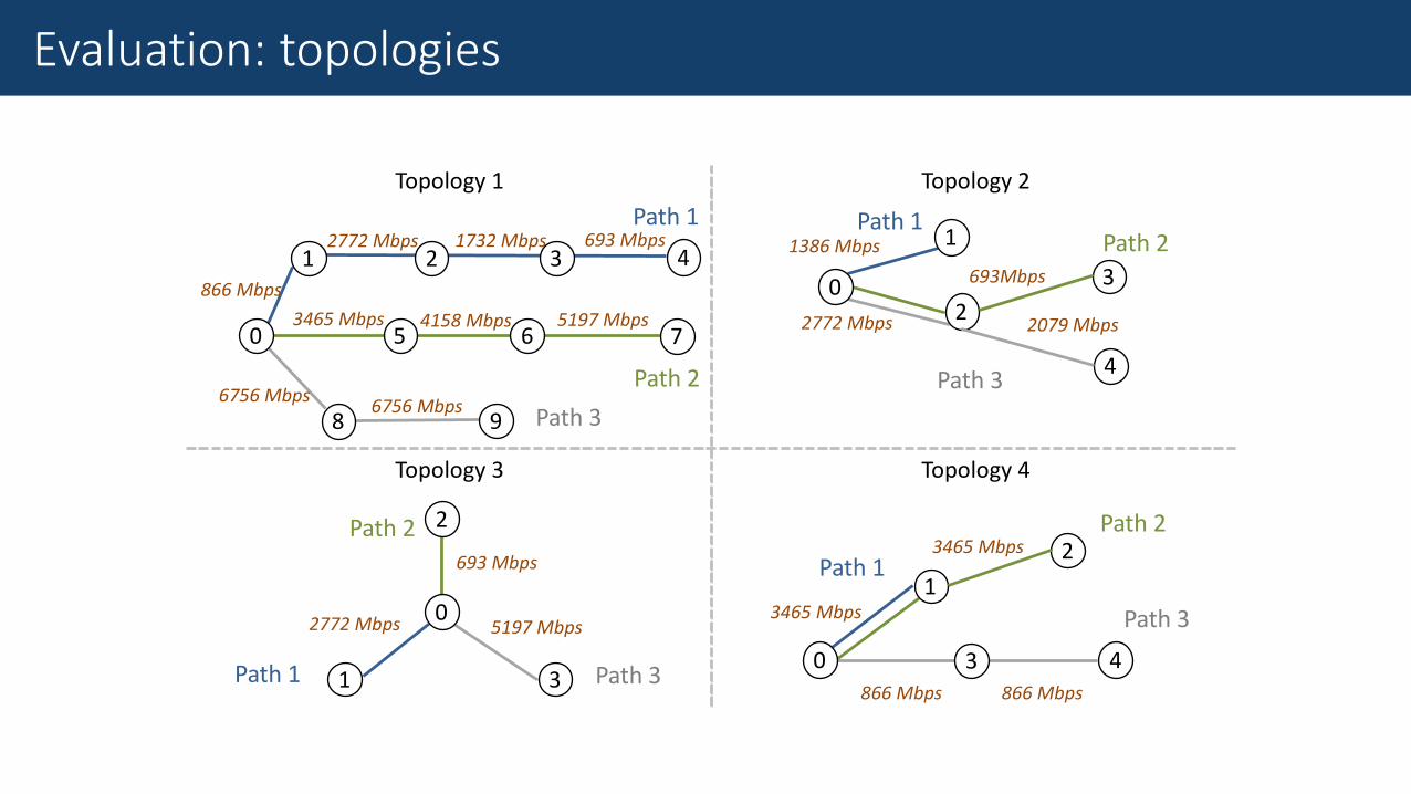
Topology1
Path2
Path3
Path1
866Mbps
6756Mbps
3465Mbps
1732Mbps 693Mbps
4158 Mbps 5197 Mbps
2772Mbps
Topology2
Topology3
Path2
Path3Path1
5197Mbps
693Mbps
2772Mbps
2
1
0
3
Path2
Path3
Path12
1
0 43866Mbps
3465Mbps
866Mbps
3465Mbps
Topology4
Path2
Path3
Path11386Mbps
2772Mbps 2
1
0 3
4
2079Mbps
693Mbps
0 5 6 7
986756Mbps
1 2 3 4
Evaluation: topologies
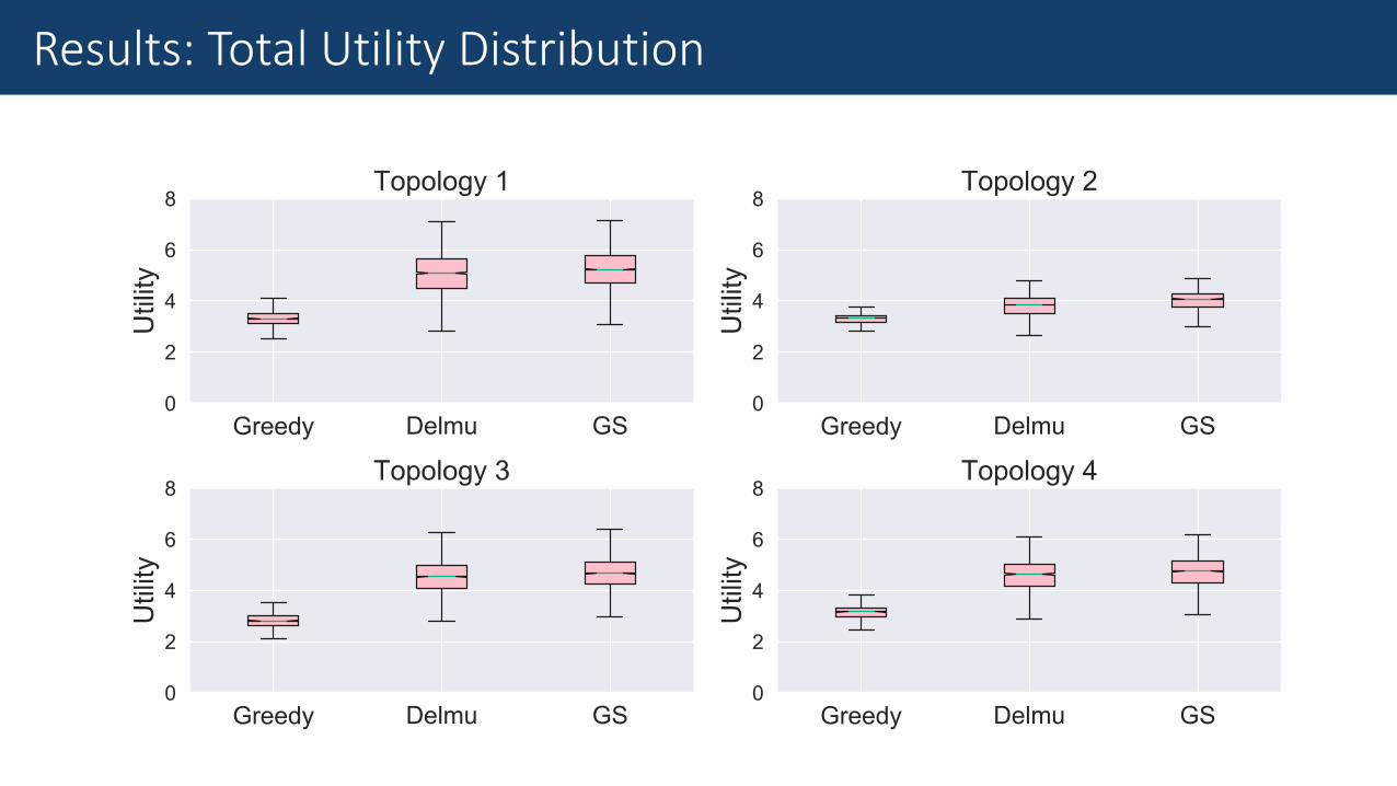
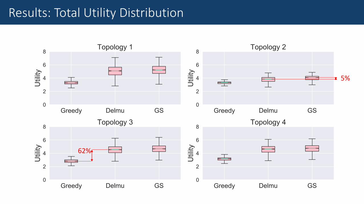
Results: Total Utility Distribution
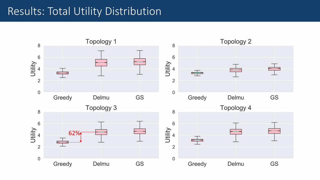
62%
Results: Total Utility Distribution
62%
5%
Results: Total Utility Distribution

Results: Utility per Traffic Type
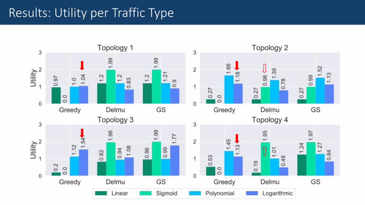
Results: Utility per Traffic Type

Results: Utility per Traffic Type

Results: Utility per Traffic Type
• Dell workstation• Average computation time over 2k instances
Computation time
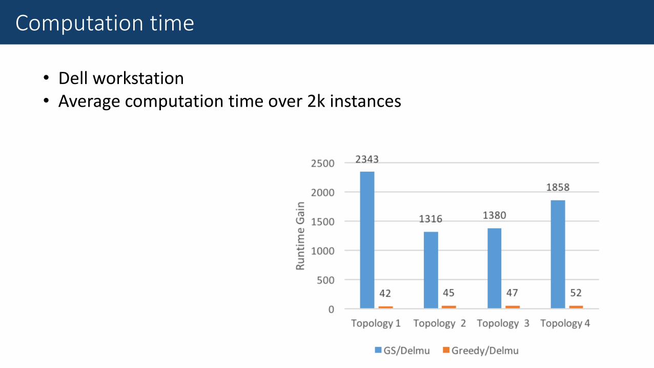
• Dell workstation• Average computation time over 2k instances
Computation time
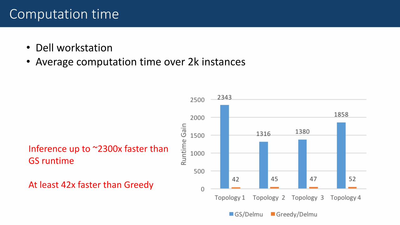
• Dell workstation• Average computation time over 2k instances
Inference up to ~2300x faster than GS runtime
At least 42x faster than Greedy
Computation time
• A general utility framework that encompasses all known types of utility functions
• Delmu achieves close-to-optimal utility solutions, and makes rapid inferences
• Suitable for 5G backhauls with real-time and dynamic requirements
Summary
R. Li, C. Zhang, P. Cao, P. Patras, J. S. Thompson, "DELMU: A Deep Learning Approach to Maximising the Utility of Virtualised Millimetre-Wave Backhauls", in Proceedings International Conference on Machine Learning for Networking (MLN), Paris, France, November 2018.


![5G NSA for SAEGW - Cisco...Standalone(NSA). configure contextcontext_name pgw-serviceservice_name [no]dcnr end NOTES: •pgw-serviceservice_name:ConfigurestheP-GWService.service_namemustbeanalphanumeric](https://img.pdfslide.net/doc/110x75/5f0affdf7e708231d42e5c02/5g-nsa-for-saegw-cisco-standalonensa-configure-contextcontextname-pgw-serviceservicename.jpg)


![RNC-A SERIES - Bakedeco RNC-210A_Manual.pdf · RNC-90A-R/L 2 RNC-120A-R/L 2 RNC-150A-R/L 3 RNC-180A-R/L 3 RNC-210A-R/L 4 [f] WATERPROOF COVER To prevent the entrance of water, the](https://img.pdfslide.net/doc/110x75/5e680bb313a66779ab666ae1/rnc-a-series-bakedeco-rnc-210amanualpdf-rnc-90a-rl-2-rnc-120a-rl-2-rnc-150a-rl.jpg)