Deep Learning for

Computer VisionLecture 8: Optimization

Peter Belhumeur

Computer Science Columbia University

Gradient-Based Optimization

f(x)

x

local minimum

global minimum

Gradient-Based Optimization

f(x)

x

x0

f(x0 + ✏) ' f(x0) + ✏f

0(x0)

x0 + ✏

f

0 =df

dx

Gradient Descent

f(x)

x

x0

f(x0 + ✏) ' f(x0) + ✏f

0(x0)

x0 + ✏

Note that is negative, so going in positive direction decreases the function.

f 0

Critical Points

Maximum Minimum Saddle Point

f(x)

x

f

0(x0) = 0

x0 x0x0

f

00(x0) < 0 f

00(x0) > 0 f

00(x0) = 0

What if our input is a vector?

• Let

• The directional derivative is the slope of the function in direction

• We can find this as at

• …or after the chain rule yields

f(x) : Rn ! R

⌘ = 0@

@⌘f(x+ ⌘u)

rx

f(x)T u

u

PLEASE DON’T FORGET

rx

f(x) =

2

66666664

@f

@x1

@f

@x2

...

@f

@xn

3

77777775

Gradient Descent• So if we move in direction the slope is

• So in what direction is the slope most negative?

• Clearly in the OPPOSITE direction of the gradient!

• And if we traverse the fcn this way then we are doing steepest descent or gradient descent.

rx

f(x)T uu

xt+1 = xt � ⌘rx

f(xt

)

The Hessian Matrix• Now we just saw that the gradient is the vector

of partial derivatives wrt each of the input variables

• What if we took second derivatives?

• To do this, we can compute the Jacobian of the gradient.

• This beast is called the Hessian!

The Hessian Matrix

H(f)(x)i,j =@

2

@xi@xjf(x)

The Hessian MatrixAt a critical point

• if all of the eigenvalues of H are positive, then point is a local minimum.

• if all of the eigenvalues of H are negative, then the point is a local maximum.

• if one or more are positive and one or more are negative, then the point is a saddle point.

(rx

f = 0) :

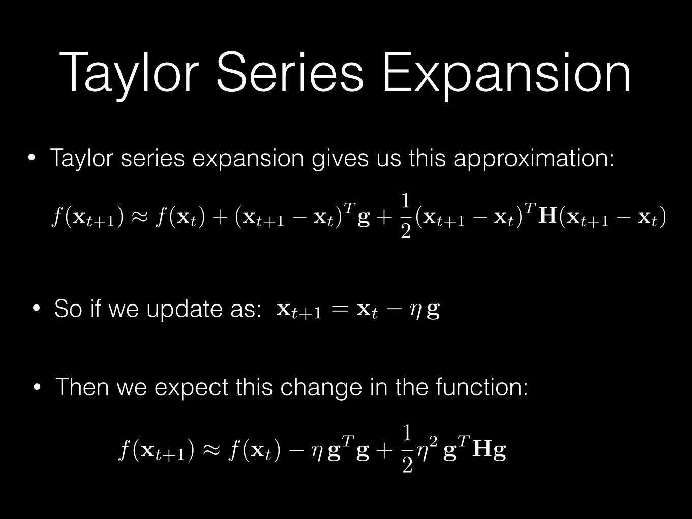
Taylor Series Expansion

f(xt+1) ⇡ f(xt) + (xt+1 � xt)Tg +

1

2(xt+1 � xt)

TH(xt+1 � xt)

xt+1 = xt � ⌘ g

f(xt+1) ⇡ f(xt)� ⌘ gTg +1

2⌘2 gTHg

• Taylor series expansion gives us this approximation:

• So if we update as:

• Then we expect this change in the function:

And that’s not all…

f(xt+1) ⇡ f(xt)� ⌘ gTg +1

2⌘2 gTHg

• Note that the second order term involving the Hessian tells us what to expect if we move in the direction of the opposite gradient.

• If the second order term is positive then the decrease in loss is diminished, and if negative it is accelerated:

Optimization for Deep Nets• Deep learning optimization is a type global optimization where the

optimization is usually expressed as a loss summed over all the training samples.

• Our goal is not so much find the parameters (or weights) that minimize the loss but rather to find parameters that produce a network with the desired behavior.

• Note that there are LOTS of solutions to which our optimization could converge to—with very different values for the weights—but each producing a model with very similar behavior on our sample data.

• For example, consider all the permutations of the weights in a hidden layer that produce the same outputs.

Optimization for Deep Nets• Although there is a seemingly endless literature on global

optimization, here we consider only gradient descent-based methods.

• Our optimizations for deep learning are typically done in very high dimensional spaces, were the parameters we are optimizing can run into the millions.

• And for these optimizations, when starting the training from scratch (i.e., some random initialization of the weights) we will needs LOTS of labeled training data.

• The process of learning our model from this labeled data is referred to as supervised learning. Although, supervised learning is more general than the deep learning algorithms we will consider.

Deterministic vs. Stochastic Methods

• If we performed our gradient descent optimization using all the training samples to compute each step in our parameter updates, then our optimization would be deterministic.

• Confusingly, deterministic gradient descent algorithms are sometimes referred to as batch algorithms

• In contrast, when we use a subset of randomly selected training samples to compute each update, we call this stochastic gradient descent and refer to the subset of samples as a mini-batch.

• And even more confusingly, we often call this mini-batch the “batch” and refer to its size as the “batch size.”

Deterministic vs. Stochastic Methods

• In general, we will have too many training samples to use deterministic methods, as it will be too computationally costly to process all samples with each update.

• Also, processing a random mini-batch serves as a type of regularization and helps prevent overfitting.

• So we will, restrict ourselves to stochastic gradient descent (SGD) from here on.

Stochastic Gradient DescentThe SGD algorithm could not be any simpler:

1. Choose a learning rate schedule.

2. Choose stopping criterion.

3. Choose batch size.

4. Randomly select a mini-batch.

5. Propagate it forward through the network and then backward through the network computing the gradient wrt the weights using back propagation.

6. Update the weights by moving in the direction opposite the gradient where the step size is given by the learning rate.

7. Repeat 4, 5, and 6 until the stopping criterion is satisfied.

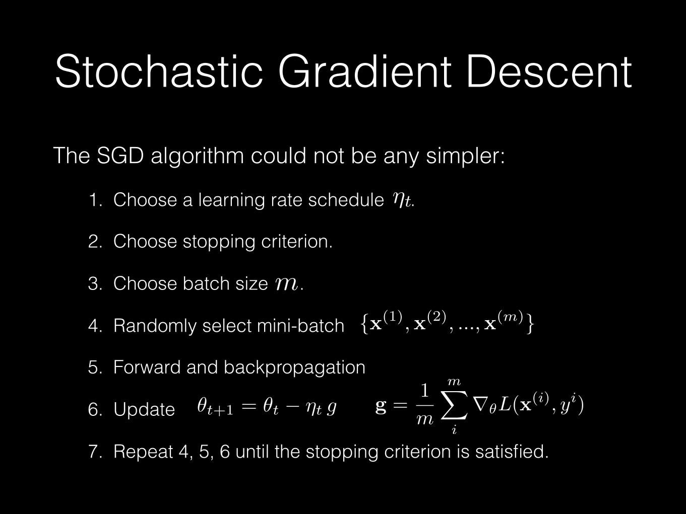
Stochastic Gradient DescentThe SGD algorithm could not be any simpler:

1. Choose a learning rate schedule .

2. Choose stopping criterion.

3. Choose batch size .

4. Randomly select mini-batch

5. Forward and backpropagation

6. Update

7. Repeat 4, 5, 6 until the stopping criterion is satisfied.

⌘t⌘t

m

{x(1),x(2), ...,x(m)}

✓t+1 = ✓t � ⌘t g g =1

m

mX

i

r✓L(x(i), yi)

SGD with Momentum

Update rule with momentum:

1. Compute the gradient:

2. Compute the velocity:

3. Update:

⌘t

✓t+1 = ✓t + vt

Note: starts small and increases with time (typically) ↵t⌘t starts large and decreases with time

vt = ↵t vt�1 � ⌘t g

g =1

m

mX

i

r✓L(x(i), yi)

Learning Rate• Choosing a learning rate has so far eluded science and remains a bit of

an art.

• A typical learning rate schedule might look like:

for

for

with equivalent to 100 - 1000 passes through the data

and

t < ⌧, ⌘t =

✓1� t

⌧

◆⌘0 +

t

⌧⌘⌧

t � ⌧, ⌘t = ⌘⌧

⌧⌘⌧ = 0.01 ⌘0

Learning Rate

• But this is just one choice for a learning schedule

• One might use an exponential decay

• Or use an adaptive learning rate…

AdaGrad • Let the learning rate for a model parameter be

inversely proportional to the square root of the sum of the square of all past values for that model parameter’s partial derivative.

• So parameters with a history of large partial derivatives get smaller step sizes, and vice versa.

• Works well sometimes, but large initial gradients can slow down the learning rates too much.

[Duchi et al. 2011]

AdaGrad

AdaGrad update rule:

1. Compute the gradient:

2. Accumulate:

3. Update parameters:

g =1

m

mX

i

r✓L(x(i), yi)

✓t+1 = ✓t �⌘

� +pst

� g

st = st�1 + g � g

RMSProp

• Similar to AdaGrad but introduces an exponential decay on the accumulation.

• Adds another hyperparameter specifying the decay rate.

• Frequently used learning rate in practice.

[Hinton 2012]

RMSProp

RMSProp update rule:

1. Compute the gradient:

2. Accumulate:

3. Update parameters:

g =1

m

mX

i

r✓L(x(i), yi)

✓t+1 = ✓t �⌘

� +pst

� g

st = � st�1 + (1� �)g � g � < 1

� = 0.9 ⌘ = 0.001Possible defaults:

Adam

• Name comes from “Adaptive moments”

• Typically not too sensitive to choice of hyperparameters.

• Frequently used learning rate in practice.

[Kingma and Ba 2014]

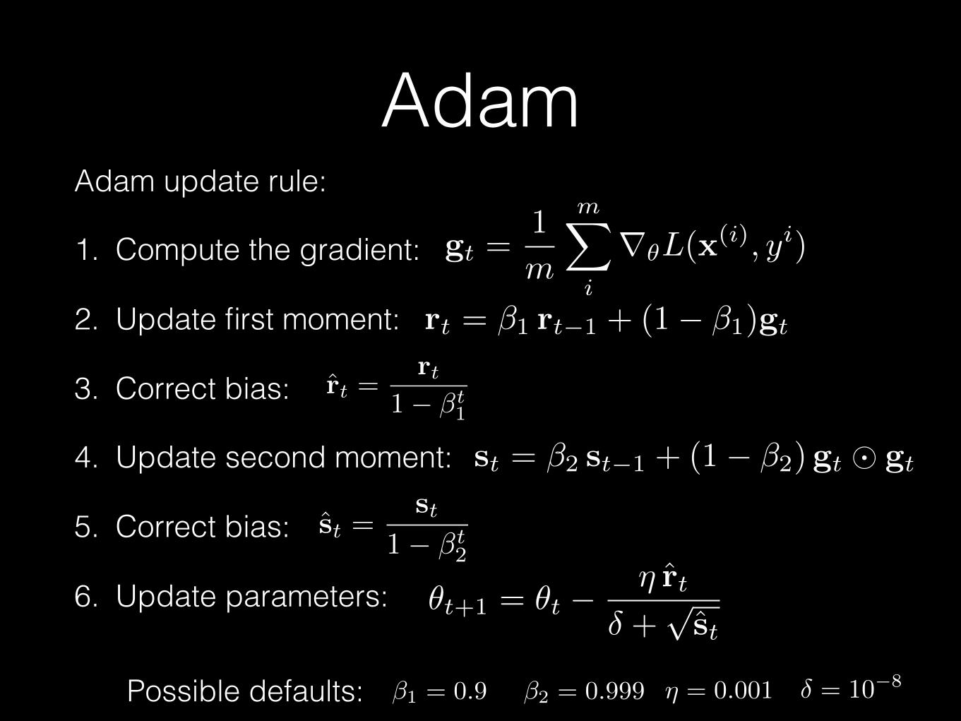
AdamAdam update rule:

1. Compute the gradient:

2. Update first moment:

3. Correct bias:

4. Update second moment:

5. Correct bias:

6. Update parameters:

st = �2 st�1 + (1� �2)gt � gt

gt =1

m

mX

i

r✓L(x(i), yi)

rt = �1 rt�1 + (1� �1)gt

rt =rt

1� �t1

st =st

1� �t2

✓t+1 = ✓t �⌘ rt

� +pst

⌘ = 0.001Possible defaults: �1 = 0.9 �2 = 0.999 � = 10�8

• Training deep nets is often tricky. Updates in weights in one layer can get compounded as stuff propagates through network.

• A recent major advance in training these networks was to normalize each batch at each unit of each layer so that it has mean = 0 and variance = 1.

• This batch normalization is usually done right before a layer’s nonlinearity.

• Scaling and bias offsets can be added back in after the normalization as explicitly learned parameters.

• Batch normalization makes training more stable and is now widely adopted.

[Ioffe and Szegedy, 2015] Batch Normalization

Batch Normalization

• Let’s say we have the input to a layer where din is the input dimension and m is the mini-batch size.

• Let the mini-batch pass through the linear part of the layer

• Note we don’t have any bias here as this will be stripped by the normalization.

X[din⇥m]

WT X = X 0[d

out

⇥m]

Batch Normalization • At this point in the network—right before the ReLu

—we are going to insert batch normalization.

• To do this, we are going to process every row of so that is has mean = 0 and variance = 1.

• Note that each unit—row of — is normalized separately to produce a new matrix

• Finally, we rescale and shift each row by broadcasting vectors and to produce

X 0

X 0

X 00

�X 00 + �� �

Batch Normalization

µ =1

m

mX

i=1

X 0:,i

X 0 = WT X

�2 =1

m

mX

i=1

(X 0:,i � µ)2

X 00:,i =

X 0:,i � µ

p�2 + ✏

X 000:,i = � �X 00

:,i + �

1.

2.

3.

4.

5.

Put input through linearity

Find the mean of each unit

Find the variance of each unit

Normalize each unit

Rescale and shift each unit

Batch Normalization

• Batch normalization just becomes another layer that can be added to the network.

• The layer is subject to both forward and back propagation!

• The scaling and offset are learned like all other weights.

� �