Deep Learning for Laser Based OdometryEstimation

Austin Nicolai, Ryan Skeele, Christopher Eriksen, and Geoffrey A. HollingerRobotics Program

School of Mechanical, Industrial, & Manufacturing EngineeringOregon State University, Corvallis, Oregon 97331

Email: {nicolaia, skeeler, eriksenc, geoff.hollinger}@oregonstate.edu

Abstract—In this paper we take advantage of recent advancesin deep learning techniques focused on image classification toestimate transforms between consecutive point clouds. A standardtechnique for feature learning is to use convolutional neuralnetworks. Leveraging this technique can help with one of thebiggest challenges in robotic motion planning, real time odometry.Sensors have advanced in recent years to provide vast amountsof precise environmental data, but localization methods can havea difficult time efficiently parsing these large quantities. In orderto address this hurdle we utilize convolution neural networksfor reducing the state space of the laser scan. We implement ournetwork in the Theano framework with the Keras wrapper. Inputdata is collected from a VLP-16 in both small office and largeopen environments. We present the results of our experiments onvarying network configurations. Our approach shows promisingresults, achieving (per direction) accuracy within 10 cm and anaverage network prediction time of 4.58 ms.

I. INTRODUCTION

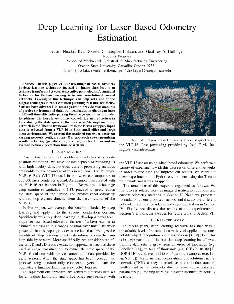
One of the most difficult problems in robotics is accurateposition estimation. We have sensors capable of providing uswith high fidelity data, however, current processing methodsare unable to take advantage of this in real-time. The VelodyneVLP-16 Puck (VLP-16) used in this work can output up to300,000 laser points per second. An example map created withthe VLP-16 can be seen in Figure 1. We propose to leveragedeep learning to capitalize on GPU processing speed, reducethe state space of the sensor, and predict robot odometrywithout loop closure directly from the laser returns of theVLP-16.

In this project, we leverage the benefits afforded by deeplearning and apply it to the robotic localization domain.Specifically we apply deep learning to develop a novel tech-nique for laser-based odometry, the use of a laser scanner toestimate the change in a robot’s position over time. The workpresented in this paper provides a method that leverages thebenefits of deep learning to estimate odometry directly fromhigh fidelity sensors. More specifically, we consider state-of-the-art 2D and 3D feature extraction approaches, such as thoseused in image classification, to reduce the state space of theVLP-16 and deal with the vast amounts of data provided bythese sensors. After the state space has been reduced, wepropose using standard fully connected layers to learn theodometry estimation from these extracted features.

To implement our approach, we generate a custom data setfor an indoor laboratory and office based environment with

Fig. 1: Map of Oregon State University’s library quad usingthe VLP-16. Post processing provided by Real Earth, Inc.http://www.realearth.us

the VLP-16 sensor using wheel based odometry. We perform avariety of experiments with this data set on different networksin order to fine tune and improve our results. We carry outthese experiments in a Python environment using the Theanoframework and Keras wrapper.

The remainder of this paper is organized as follows. Wefirst discuss related work in image classification domains andcurrent odometry methods in Section II. Next, we present aformulation of our proposed method and discuss the differentnetwork structures considered and experimented on in SectionIV. Finally, we discuss the results of our experiments inSection V and discuss avenues for future work in Section VII.

II. RELATED WORK

In recent years, deep learning research has met with aremarkable level of success in a variety of applications, mostnotably object recognition and classification [8] [9] [17]. Thisis in large part due to the fact that deep learning has allowedtraining data sets to grow from an order of thousands (e.g.LabelMe [14]), to tens of thousands (e.g. CIFAR-10/100 [7],NORB [10]), and even millions of training examples (e.g. Im-ageNet [3]). Many such networks utilize convolutional neuralnetworks (CNNs) as they are much easier to train than standardfeedforward neural networks due to fewer connections andparameters [9], making learning in a deep architecture actuallyfeasible.

Wheel based odometry utilizes encoders on a robot’swheels, factoring wheel rotation into a forward kinematicmodel to estimate the motion of the robotic base. This processis known as dead reckoning, and is known to result in adiverging estimate of a robot’s position over time due tothe fact that odometry errors are compounded over time. Forthis reason, localization methods usually combine odometrymeasures with some form of absolute position measure (e.g.using laser scanner returns to estimate a robot’s position ina pre-constructed map) to keep errors from diverging. Inaddition to wheel encoders, classical odometry measures oftenuse an IMU, a combination of a three accelerometers andgyroscopres. Both of these measures are often known to givenoisy estimates however, the most prominent source of whichis wheel slippage.

One method to circumvent these kinds of errors is a processknown as scan-matching (e.g. [11] [18]), which often uses atechnique known as Iterative Closest Point (ICP) [2] to itera-tively minimize the difference between two clouds of points,in this case two consecutively laser scans. The estimatedtransformation is used to estimate the motion of the roboticbase. Despite popular use and developments in efficiency,ICP is still expensive to compute and furthermore sensitiveto large differences in the initial point distributions, as thecorrect point correspondence is difficult to find. We note recentsuccess by Zhang and Singh [19] [20] in achieving low-drift,real-time odometry using scan-matching by simultaneouslyrunning two algorithms - one that runs at a fast rate butperforms only course matching and another that runs an orderof magnitude slower but performs fine grained matching andpoint registration. The fidelity achieved in this approach ableto maintain accurate position estimates over time without theuse of external, absolute position measures.

Another technique that has met with success is visualodometry (e.g. [1], [13]), a process that uses image featuresto estimate the ego-motion of a camera. While sensitive tofeatures used in image processing, recent performance im-provements on image-based applications (particularly with the

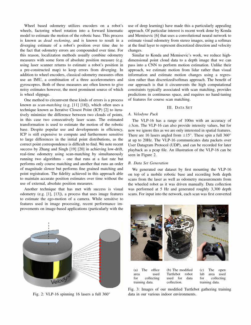
Fig. 2: VLP-16 spinning 16 lasers a full 360◦

use of deep learning) have made this a particularly appealingapproach. Of particular interest is recent work done by Kondaand Memisevic [6] that uses a convolutional neural network toestimate visual odometry from stereo images, using a softmaxat the final layer to represent discretized direction and velocitychanges.

Similar to Konda and Memisevic’s work, we reduce high-dimensional point cloud data to a depth image that we canpass into a CNN to perform motion estimation. Unlike theirapproach, we estimate motion from lidar rather than visualinformation and estimate motion changes using a regres-sion rather than discretized/softmax approach. The benefit ofour approach is that it circumvents the high computationalconstraints typically associated with scan matching, providespredictions in continuous space, and requires no hand-tuningof features for course scan matching.

III. DATA SET

A. Velodyne Puck

The VLP-16 has a range of 100m with an accuracy of±3cm. The VLP-16 can also provide intensity values, but fornow we ignore this as we are only interested in spatial features.There are 16 lasers angled from ±15◦. These spin a full 360◦

at up to 20Hz. The VLP-16 communicates data packets overUser Datagram Protocol (UDP), and can be recorded for laterplayback as a pcap file. An illustration of the VLP-16 can beseen in Figure 2.

B. Data Set Generation

We generated our dataset by first mounting the VLP-16on top of a mobile robotic base and recording both depthscans from the laser as well as odometry measurements fromthe wheeled robot as it was driven manually. Data collectionwas performed at 5 Hz and generated roughly 3,300 depthscans. For input into the network, each scan was first converted

(a) The officearea usedfor collectingtraining data.

(b) The modifiedTurtlebot robotused for datacollection.

(c) The openlab area usedfor collectingtraining data.

Fig. 3: Images of our modified Turtlebot gathering trainingdata in our various indoor environments.

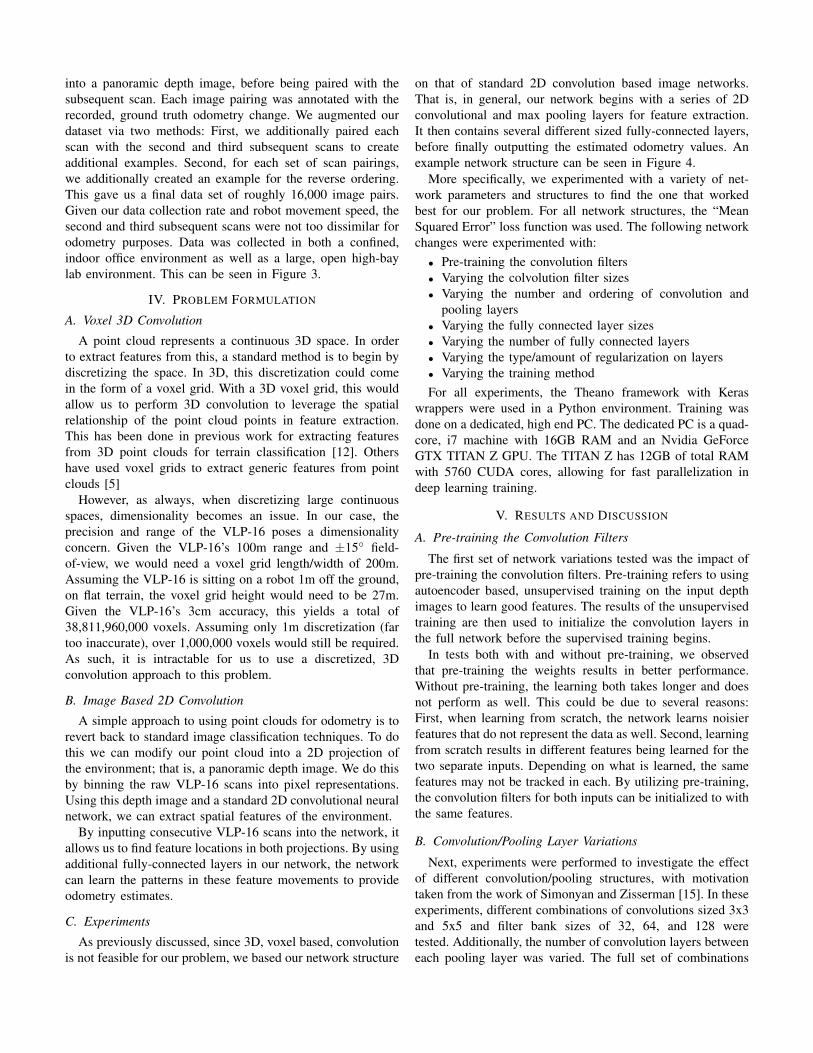
into a panoramic depth image, before being paired with thesubsequent scan. Each image pairing was annotated with therecorded, ground truth odometry change. We augmented ourdataset via two methods: First, we additionally paired eachscan with the second and third subsequent scans to createadditional examples. Second, for each set of scan pairings,we additionally created an example for the reverse ordering.This gave us a final data set of roughly 16,000 image pairs.Given our data collection rate and robot movement speed, thesecond and third subsequent scans were not too dissimilar forodometry purposes. Data was collected in both a confined,indoor office environment as well as a large, open high-baylab environment. This can be seen in Figure 3.

IV. PROBLEM FORMULATION

A. Voxel 3D Convolution

A point cloud represents a continuous 3D space. In orderto extract features from this, a standard method is to begin bydiscretizing the space. In 3D, this discretization could comein the form of a voxel grid. With a 3D voxel grid, this wouldallow us to perform 3D convolution to leverage the spatialrelationship of the point cloud points in feature extraction.This has been done in previous work for extracting featuresfrom 3D point clouds for terrain classification [12]. Othershave used voxel grids to extract generic features from pointclouds [5]

However, as always, when discretizing large continuousspaces, dimensionality becomes an issue. In our case, theprecision and range of the VLP-16 poses a dimensionalityconcern. Given the VLP-16’s 100m range and ±15◦ field-of-view, we would need a voxel grid length/width of 200m.Assuming the VLP-16 is sitting on a robot 1m off the ground,on flat terrain, the voxel grid height would need to be 27m.Given the VLP-16’s 3cm accuracy, this yields a total of38,811,960,000 voxels. Assuming only 1m discretization (fartoo inaccurate), over 1,000,000 voxels would still be required.As such, it is intractable for us to use a discretized, 3Dconvolution approach to this problem.

B. Image Based 2D Convolution

A simple approach to using point clouds for odometry is torevert back to standard image classification techniques. To dothis we can modify our point cloud into a 2D projection ofthe environment; that is, a panoramic depth image. We do thisby binning the raw VLP-16 scans into pixel representations.Using this depth image and a standard 2D convolutional neuralnetwork, we can extract spatial features of the environment.

By inputting consecutive VLP-16 scans into the network, itallows us to find feature locations in both projections. By usingadditional fully-connected layers in our network, the networkcan learn the patterns in these feature movements to provideodometry estimates.

C. Experiments

As previously discussed, since 3D, voxel based, convolutionis not feasible for our problem, we based our network structure

on that of standard 2D convolution based image networks.That is, in general, our network begins with a series of 2Dconvolutional and max pooling layers for feature extraction.It then contains several different sized fully-connected layers,before finally outputting the estimated odometry values. Anexample network structure can be seen in Figure 4.

More specifically, we experimented with a variety of net-work parameters and structures to find the one that workedbest for our problem. For all network structures, the “MeanSquared Error” loss function was used. The following networkchanges were experimented with:

• Pre-training the convolution filters• Varying the colvolution filter sizes• Varying the number and ordering of convolution and

pooling layers• Varying the fully connected layer sizes• Varying the number of fully connected layers• Varying the type/amount of regularization on layers• Varying the training methodFor all experiments, the Theano framework with Keras

wrappers were used in a Python environment. Training wasdone on a dedicated, high end PC. The dedicated PC is a quad-core, i7 machine with 16GB RAM and an Nvidia GeForceGTX TITAN Z GPU. The TITAN Z has 12GB of total RAMwith 5760 CUDA cores, allowing for fast parallelization indeep learning training.

V. RESULTS AND DISCUSSION

A. Pre-training the Convolution Filters

The first set of network variations tested was the impact ofpre-training the convolution filters. Pre-training refers to usingautoencoder based, unsupervised training on the input depthimages to learn good features. The results of the unsupervisedtraining are then used to initialize the convolution layers inthe full network before the supervised training begins.

In tests both with and without pre-training, we observedthat pre-training the weights results in better performance.Without pre-training, the learning both takes longer and doesnot perform as well. This could be due to several reasons:First, when learning from scratch, the network learns noisierfeatures that do not represent the data as well. Second, learningfrom scratch results in different features being learned for thetwo separate inputs. Depending on what is learned, the samefeatures may not be tracked in each. By utilizing pre-training,the convolution filters for both inputs can be initialized to withthe same features.

B. Convolution/Pooling Layer Variations

Next, experiments were performed to investigate the effectof different convolution/pooling structures, with motivationtaken from the work of Simonyan and Zisserman [15]. In theseexperiments, different combinations of convolutions sized 3x3and 5x5 and filter bank sizes of 32, 64, and 128 weretested. Additionally, the number of convolution layers betweeneach pooling layer was varied. The full set of combinations

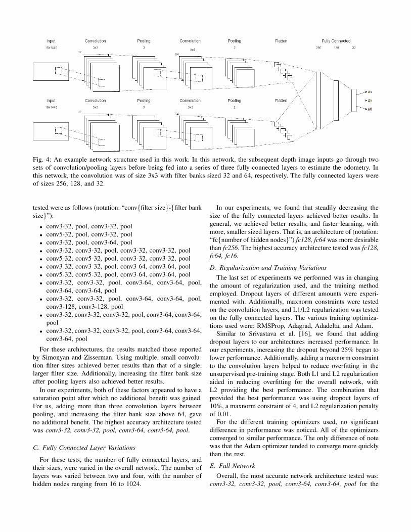
Fig. 4: An example network structure used in this work. In this network, the subsequent depth image inputs go through twosets of convolution/pooling layers before being fed into a series of three fully connected layers to estimate the odometry. Inthis network, the convolution was of size 3x3 with filter banks sized 32 and 64, respectively. The fully connected layers wereof sizes 256, 128, and 32.

tested were as follows (notation: “conv{filter size}-{filter banksize}”):

• conv3-32, pool, conv3-32, pool• conv5-32, pool, conv3-32, pool• conv3-32, pool, conv3-64, pool• conv3-32, conv3-32, pool, conv3-32, conv3-32, pool• conv5-32, conv5-32, pool, conv3-32, conv3-32, pool• conv3-32, conv3-32, pool, conv3-64, conv3-64, pool• conv5-32, conv5-32, pool, conv3-64, conv3-64, pool• conv3-32, conv3-32, pool, conv3-64, conv3-64, pool,

conv3-64, conv3-64, pool• conv3-32, conv3-32, pool, conv3-64, conv3-64, pool,

conv3-128, conv3-128, pool• conv3-32, conv3-32, conv3-32, pool, conv3-64, conv3-64,

pool• conv3-32, conv3-32, conv3-32, pool, conv3-64, conv3-64,

conv3-64, pool

For these architectures, the results matched those reportedby Simonyan and Zisserman. Using multiple, small convolu-tion filter sizes achieved better results than that of a single,larger filter size. Additionally, increasing the filter bank sizeafter pooling layers also achieved better results.

In our experiments, both of these factors appeared to have asaturation point after which no additional benefit was gained.For us, adding more than three convolution layers betweenpooling, and increasing the filter bank size above 64, gaveno additional benefit. The highest accuracy architecture testedwas conv3-32, conv3-32, pool, conv3-64, conv3-64, pool.

C. Fully Connected Layer Variations

For these tests, the number of fully connected layers, andtheir sizes, were varied in the overall network. The number oflayers was varied between two and four, with the number ofhidden nodes ranging from 16 to 1024.

In our experiments, we found that steadily decreasing thesize of the fully connected layers achieved better results. Ingeneral, we achieved better results, and faster learning, withmore, smaller sized layers. That is, an architecture of (notation:“fc{number of hidden nodes}”) fc128, fc64 was more desirablethan fc256. The highest accuracy architecture tested was fc128,fc64, fc16.

D. Regularization and Training Variations

The last set of experiments we performed was in changingthe amount of regularization used, and the training methodemployed. Dropout layers of different amounts were experi-mented with. Additionally, maxnorm constraints were testedon the convolution layers, and L1/L2 regularization was testedon the fully connected layers. The various training optimiza-tions used were: RMSProp, Adagrad, Adadelta, and Adam.

Similar to Srivastava et al. [16], we found that addingdropout layers to our architectures increased performance. Inour experiments, increasing the dropout beyond 25% began tolower performance. Additionally, adding a maxnorm constraintto the convolution layers helped to reduce overfitting in theunsupervised pre-training stage. Both L1 and L2 regularizationaided in reducing overfitting for the overall network, withL2 providing the best performance. The combination thatprovided the best performance was using dropout layers of10%, a maxnorm constraint of 4, and L2 regularization penaltyof 0.01.

For the different training optimizers used, no significantdifference in performance was noticed. All of the optimizersconverged to similar performance. The only difference of notewas that the Adam optimizer tended to converge more quicklythan the rest.

E. Full Network

Overall, the most accurate network architecture tested was:conv3-32, conv3-32, pool, conv3-64, conv3-64, pool for the

feature extraction stage and fc128, fc64, fc16 for the fullyconnected stage. The network used dropout layers of 10%, amaxnorm constraint of 4 on the convolution layers, and an L2regularization penalty of 0.01 on the fully connected layers.Additionally, it took advantage of unsupervised pre-training toseed the convolution filters in the full network.

For the test data set, this network architecture achieved anaverage odometry estimate error of 0.0763 m, or 7.63 cm. Thisrepresented a roughly 30% error in the estimate. Across thetest set, the largest error measured was 0.611 m, or 61.1 cm.On average, the network took 4.58 ms to provide an estimate.

VI. CONCLUSION

While the preliminary results presented here are not ableto compete with state-of-the-art scan matching techniques, wecan conclude that the architecture presented is able to providereasonable odometry estimates from large scale lidar data.While the current results have room for improvement, the perscan pair estimate time of the network is promising. We believethat this work is a step towards leveraging deep learning forefficient use of high fidelity sensor data.

VII. FUTURE WORK

Moving forward, the authors have several avenues theywould like to pursue as future work. These avenues addressthe challenges of increasing the accuracy of these results, andrealizing this work on actual robots in the field.

The first avenue involves exploring additional network struc-tures/parameters to increase prediction accuracy. One possibil-ity is to discretize the predictions and formulate the networkas a classifier. To address the loss of precision, classificationranges could be intelligently chosen based on the spread ofvalues represented in the data set. In this case, a separatenetwork for each degree of freedom could be trained, similar toKonda and Memisevic [6]. Additionally, exploring the additionof LSTMs into the network architecture may allow for a moreintelligent prediction. LSTMs may allow for the network tolearn information about the robot’s dynamics, resulting in amore accurate odometry prediction when given a sequence oflidar scans.

Next, the authors are interested in creating a method thatallows us to do 3D, spatial feature extraction directly on pointcloud data. This directly addresses the issues we encounteredwith creating voxel grids of the entire space spanned by theVLP-16 while allowing for the true 3D spatial relationshipsto be leveraged rather than projected into 2D. In addressingthis issue, the authors propose implementing 3D convolutionaland pooling layers using nearest-neighbors and clusteringtechniques.

Lastly, we wish to create a more robust, and realistic, dataset. The authors propose attaching the VLP-16 to DJI Matricequadcopters [4]. This would allow for the collection of data ina full 6 degrees of freedom. Additionally, data can be collectedin a wider variety of environments and features can be viewedfrom a larger variety of angles.

VIII. ACKNOWLEDGMENTS

This research has been funded in part by the following:NASA grant NNX14AI10G, DWFritz Automation, and theOregon Metals Initiative.

REFERENCES

[1] Jason Campbell, Rahul Sukthankar, and Illah Nour-bakhsh. Techniques for evaluating optical flow for visualodometry in extreme terrain. In Proceedings of theIEEE/RSJ International Conference on Intelligent Robotsand Systems (IROS), 2004.

[2] Yang Chen and Gerard Medioni. Object modeling byregistration of multiple range images. In Proceedingsof the IEEE International Conference on Robotics andAutomation (ICRA), April 1991.

[3] Jia Deng, Wei Dong, Richard Socher, Li jia Li, KaiLi, and Li Fei-fei. Imagenet: A large-scale hierarchicalimage database. In In CVPR, 2009.

[4] DJI. Matrice 100, 2016. URL http://www.dji.com/product/matrice100.

[5] Jens Garstka and Gabriele Peters. Fast and robust key-point detection in unstructured 3-d point clouds. In Infor-matics in Control, Automation and Robotics (ICINCO),2015 12th International Conference on, volume 2, pages131–140. IEEE, 2015.

[6] Kishore Konda and Roland Memisevic. Learning visualodometry with a convolutional network. In InternationalConference on Computer Vision Theory and Applica-tions), 2015.

[7] Alex Krizhevsky. Learning Multiple Layers of Featuresfrom Tiny Images. Master’s thesis, University of Toronto,Department of Computer Science, 2009.

[8] Alex Krizhevsky. Convolutional deep belief networks oncifar-10. 2010. Unpublished manuscript.

[9] Alex Krizhevsky, Ilya Sutskever, and Geoffrey E. Hinton.Imagenet classification with deep convolutional neuralnetworks. In F. Pereira, C.J.C. Burges, L. Bottou, andK.Q. Weinberger, editors, Advances in Neural Informa-tion Processing Systems 25, pages 1097–1105. CurranAssociates, Inc., 2012.

[10] Y. LeCun, Fu Jie Huang, and L. Bottou. Learningmethods for generic object recognition with invarianceto pose and lighting. In Computer Vision and PatternRecognition, 2004. CVPR 2004. Proceedings of the 2004IEEE Computer Society Conference on, volume 2, pagesII–97–104 Vol.2, June 2004. doi: 10.1109/CVPR.2004.1315150.

[11] Feng Lu. Shape Registration using Optimization forMobile Robot Navigation. PhD thesis, University ofToronto, 1995.

[12] Daniel Maturana and Sebastian Scherer. 3d convolutionalneural networks for landing zone detection from lidar.In Robotics and Automation (ICRA), 2015 IEEE Inter-national Conference on, pages 3471–3478. IEEE, 2015.

[13] David Nister, Oleg Naroditsky, and James Bergen. Visual

odometry. In Computer Vision and Pattern Recognition(CVPR), 2004.

[14] Bryan C. Russell, Antonio Torralba, Kevin P. Murphy,and William T. Freeman. Labelme: A database and web-based tool for image annotation. Int. J. Comput. Vision,77(1-3):157–173, May 2008. ISSN 0920-5691. doi: 10.1007/s11263-007-0090-8.

[15] K. Simonyan and A. Zisserman. Very deep convolu-tional networks for large-scale image recognition. CoRR,abs/1409.1556, 2014.

[16] Nitish Srivastava, Geoffrey Hinton, Alex Krizhevsky,Ilya Sutskever, and Ruslan Salakhutdinov. Dropout: Asimple way to prevent neural networks from overfitting.The Journal of Machine Learning Research, 15(1):1929–1958, 2014.

[17] Oriol Vinyals, Alexander Toshev, Samy Bengio, andDumitru Erhan. Show and tell: A neural image captiongenerator. 2014.

[18] G. Weiss and E. Puttkamer. A map based on laserscanswithout geometric interpretation. Intelligent AutonomousSystems, pages 403–407, 1995.

[19] Ji Zhang and Sanjiv Singh. Loam: Lidar odometry andmapping in real-time. In Robotics: Science and SystemsConference (RSS), 2014.

[20] Ji Zhang and Sanjiv Singh. Low-drift and real-time lidarodometry and mapping. Autonomous Robots, 10.1007,2016.