Deep Learning Neural Network-based Sinogram

Interpolation for Sparse-View CT Reconstruction

Swapnil Vekhande

Thesis submitted to the Faculty of the Virginia Polytechnic Institute and State

University in partial fulfillment of the requirements for the degree of

Master of Science

in

Computer Engineering

Guohua Cao, Co-Chair

A. Lynn Abbott, Co-Chair

Jia-Bin Huang

April 30, 2019

Blacksburg, Virginia Keywords: Medical Imaging, Image Reconstruction, Deep Learning

Deep Learning Neural Network-based Sinogram

Interpolation for Sparse-View CT Reconstruction

Swapnil Vekhande

(ABSTRACT)

Computed Tomography (CT) finds applications across domains like medical diagnosis, security

screening, and scientific research. In medical imaging, CT allows physicians to diagnose injuries

and disease more quickly and accurately than other imaging techniques. However, CT is one of

the most significant contributors of radiation dose to the general population and the required

radiation dose for scanning could lead to cancer. On the other hand, a shallow radiation dose could

sacrifice image quality causing misdiagnosis. To reduce the radiation dose, sparse-view CT, which

includes capturing a smaller number of projections, becomes a promising alternative. However,

the image reconstructed from linearly interpolated views possesses severe artifacts.

Recently, Deep Learning-based methods are increasingly being used to interpret the missing data

by learning the nature of the image formation process. The current methods are promising but

operate mostly in the image domain presumably due to lack of projection data. Another limitation

is the use of simulated data with less sparsity (up to 75%). This research aims to interpolate the

missing sparse-view CT in the sinogram domain using deep learning. To this end, a residual U-

Net architecture has been trained with patch-wise projection data to minimize Euclidean distance

between the ground truth and the interpolated sinogram. The model can generate highly sparse

missing projection data. The results show improvement in SSIM and RMSE by 14% and 52%

respectively with respect to the linear interpolation-based methods. Thus, experimental sparse-

view CT data with 90% sparsity has been successfully interpolated while improving CT image

quality.

Deep Learning Neural Network-based Sinogram

Interpolation for Sparse-View CT Reconstruction

Swapnil Vekhande

(GENERAL AUDIENCE ABSTRACT)

Computed Tomography is a commonly used imaging technique due to the remarkable ability to

visualize internal organs, bones, soft tissues, and blood vessels. It involves exposing the subject to

X-ray radiation, which could lead to cancer. On the other hand, the radiation dose is critical for the

image quality and subsequent diagnosis. Thus, image reconstruction using only a small number of

projection data is an open research problem.

Deep learning techniques have already revolutionized various Computer Vision applications.

Here, we have used a method which fills missing highly sparse CT data. The results show that the

deep learning-based method outperforms standard linear interpolation-based methods while

improving the image quality.

v

Dedication

This dissertation is dedicated to all those who give up dreams of higher education due to family

responsibilities.

vi

Acknowledgments

Foremost, I would like to express my utmost gratitude to my academic advisor Dr. Guohua Cao

for his patience and perseverance while advising me. He has put in a tremendous amount of efforts

in guiding and motivating me to do this research.

This interdepartmental research was made possible due to the courtesy of Dr. A. Lynn Abbott. He

also guided me through writing. I gratefully thank Dr. Paul Plassmann, for providing me with

unwavering support. I also give many thanks to Dr. Jia-Bin Huang for his invaluable insights and

mentorship during the year.

I would also extend my thanks to Xu Dong from Biomedical Engineering, who was always there

to help me out.

I am also thankful to my family for all the support.

Lastly, I thank the almighty for providing me the opportunity.

vii

Contents

List of Figures ix

List of Tables xi

List of Abbreviations xii

1 INTRODUCTION 1

1.1 Computed Tomography 1

1.2 Sinogram Synthesis 3

1.3 Image Reconstruction Principles 4

1.4 Filtered BackProjection 7

1.4 Sparse CT Reconstruction Literature 8

1.5 Organization of Thesis 9

2 METHODS AND EXPERIMENTS 11

2.1 Data Preparation 11

2.2 The Residual U-Net Architecture 13

2.3 Training 15

viii

2.4 Implementation Details 16

3 RESULTS 18

3.1 Evaluation in the Sinogram Domain 18

3.2 Evaluation in the Image Domain 19

3.3 Quantitative Comparison of the Results 21

4 DISCUSSION AND CONCLUSIONS 24

5 FUTURE DIRECTIONS 25

BIBLIOGRAPHY 26

Appendix A PUBLICATION INFORMATION 29

ix

List of Figures

1.1 The block diagram of the CT imaging system. 3

1.2 Radon transform of a point source. 3

1.3 The central slice theorem. 5

1.4 BackProjection leads to a blurred reconstructed image. 6

1.5 Filtered BackProjection with the sharp reconstructed image. 7

1.6 The frequency spectrum of Ram-Lak filter. 8

2.1 A sample projection view of the rat body scan. 11

2.2 The architecture of residual U-Net. 14

2.3 Schematic relation between ground truth, interpolation, and

correction from the model.

17

3.1 Comparison of the interpolated sinogram, the reference sinogram, and the

corrected sinogram.

18

3.2 Difference between interpolated and output sinogram with respect to

the ground truth.

19

3.3 Reconstructed images of the interpolated, the corrected, and the

truth.

20

3.4 Zoomed in central globular structure in mouse anatomy (a)

Interpolated (b) Corrected (c) Ground truth.

20

x

3.5 Comparison of interpolated image and deep learning-based

correction with respect to the ground truth.

21

3.6 Central vertical line profile comparison. 22

xi

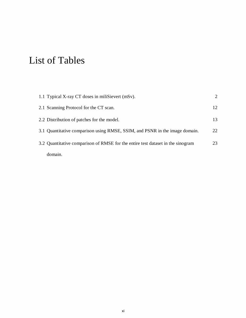
List of Tables

1.1 Typical X-ray CT doses in miliSievert (mSv). 2

2.1 Scanning Protocol for the CT scan. 12

2.2 Distribution of patches for the model. 13

3.1 Quantitative comparison using RMSE, SSIM, and PSNR in the image domain. 22

3.2 Quantitative comparison of RMSE for the entire test dataset in the sinogram

domain.

23

xii

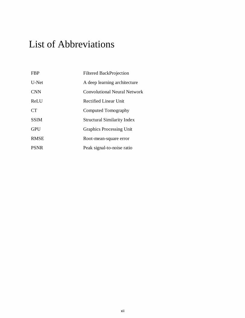
List of Abbreviations

FBP Filtered BackProjection

U-Net A deep learning architecture

CNN Convolutional Neural Network

ReLU Rectified Linear Unit

CT Computed Tomography

SSIM

GPU

Structural Similarity Index

Graphics Processing Unit

RMSE Root-mean-square error

PSNR Peak signal-to-noise ratio

1

Chapter 1

INTRODUCTION

1.1 Computed Tomography

X-ray imaging has been used in common medical exams to study anatomy. When it comes to the

3D study of biological structure, modern imaging methods like CT are imperative. A CT scan

involves combinations of an array of X-ray images taken at various angles around the body. CT

can generate cross-sectional images with fine details. CT marked the advent of volumetric analysis.

As per tomographic principles of imaging, these cross-sections are then stacked together to get a

3D representation. CT machines could use helical or fan-beam projections.

CT can help cure cancer by providing the exact stage of cancer. It helps the physician take a call

if the surgery is essential. It has helped drastically reduce length as well as the cost of

hospitalization for patients. It can help draw a radiation therapy plan by detecting the exact nature

and the presence of a tumor.

The radiation dose is dependent upon factors like the construction of the scanner, scanning

protocol, patient size, etc. The typical radiation doses[1] are listed in table 1.1.

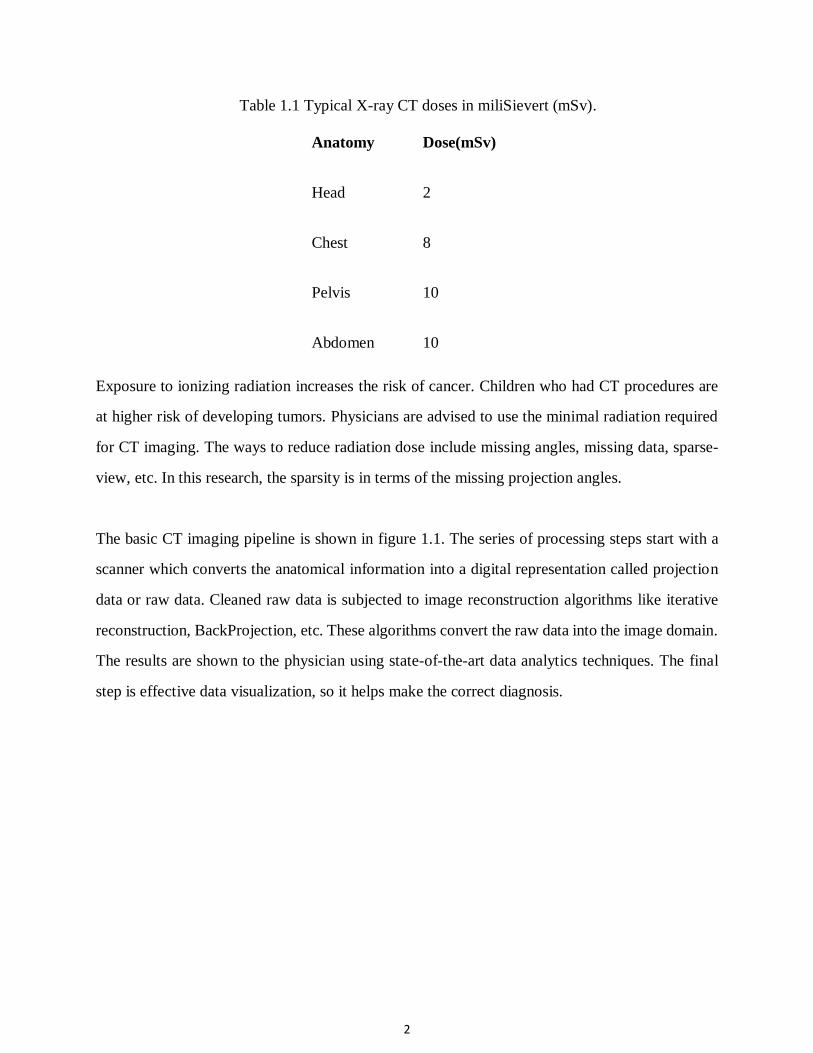
2

Table 1.1 Typical X-ray CT doses in miliSievert (mSv).

Anatomy Dose(mSv)

Head 2

Chest 8

Pelvis 10

Abdomen 10

Exposure to ionizing radiation increases the risk of cancer. Children who had CT procedures are

at higher risk of developing tumors. Physicians are advised to use the minimal radiation required

for CT imaging. The ways to reduce radiation dose include missing angles, missing data, sparse-

view, etc. In this research, the sparsity is in terms of the missing projection angles.

The basic CT imaging pipeline is shown in figure 1.1. The series of processing steps start with a

scanner which converts the anatomical information into a digital representation called projection

data or raw data. Cleaned raw data is subjected to image reconstruction algorithms like iterative

reconstruction, BackProjection, etc. These algorithms convert the raw data into the image domain.

The results are shown to the physician using state-of-the-art data analytics techniques. The final

step is effective data visualization, so it helps make the correct diagnosis.

3

Figure 1.1 The block diagram of the CT imaging system.

1.2 Sinogram Synthesis

Radon transform represents an image using a combination of projections within various directions.

A topological space qualifies as Radon if every Borel measure is a Radon measure. A Borel

measure is a measure which is defined on all open sets. Figure 1.2 shows how a single projection

at an angle 𝜙 of a point source contributes to a row in the Radon space.

Figure 1.2 Radon transform of a point source.

4

As the point traces a sine curve in the Radon space, the projection is known as a sinogram. In a

sinogram, the maximum deviation from the center indicates an object’s distance from the origin,

and the point of peak deviation indicates the angular location of the object. In general, the Radon

transform of a spatial distribution 𝑓(𝑥, 𝑦) is given as follows:

ℛ𝑓(𝜙, 𝑡) = ∫ 𝑓(𝑥, 𝑦)𝑑𝑠𝐿(𝜙,𝑡)

(1.1)

where 𝐿(𝜙, 𝑡) = {(𝑥, 𝑦)𝜖ℝ × ℝ: 𝑥 cos 𝜙 + 𝑦 sin 𝜙 = 𝑡}.

1.3 Image Reconstruction Principles

The mathematical process that reconstructs an image from the X-ray projection data tries to

minimize the error between the actual and the projected image. There are two types of

reconstruction, namely: 1) Analytical and 2) Iterative. Analytical reconstruction uses a closed form

solution quickly using mathematical transform. Iterative reconstruction tries to minimize an

objective function during each iteration hence requires more computations than the analytical

method.

This project uses Filtered BackProjection (FBP), which is explained below. Before discussing FBP

in detail, an overview of the inverse problem and the Central slice theorem is given.

Computed Tomography produces images indirectly. To this end, the mathematical formulation of

the underlying imaging physics is used to form the original image. In the sense of Hadamard’s

laws, if a mathematical model fails to satisfy any of the following three conditions, it is categorized

as an ill-posed inverse problem. The conditions are:

1. a solution exists,

2. the solution is unique,

3. the solution’s behavior changes with initial conditions.

Medical imaging science often fails to satisfy the last criterion.

5

Let 𝑋𝑒𝑥𝑎𝑐𝑡 = [𝑋𝑒𝑥𝑎𝑐𝑡1, 𝑋𝑒𝑥𝑎𝑐𝑡2, ⋯ , 𝑋𝑒𝑥𝑎𝑐𝑡𝑁]𝑇denote a exact linear attenuation coefficient

distribution that need to estimated, where 𝑁 is the total number of the pixels in a reconstructed

image. Thus, the CT image reconstruction problem can be expressed in a linear system of equations

as follows:

𝑔 = A𝑋𝑒𝑥𝑎𝑐𝑡 + 𝜎 (1.2)

where A is the system matrix, 𝑋 is the unknown image, and 𝜎 is the system noise.

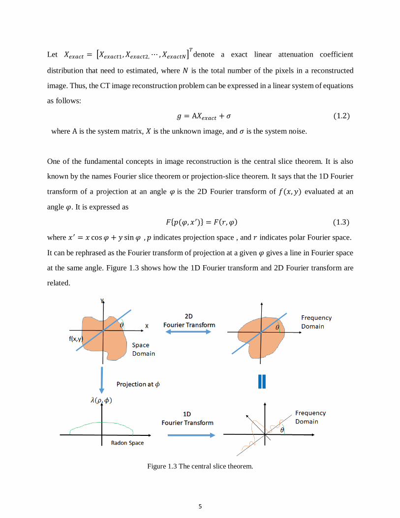
One of the fundamental concepts in image reconstruction is the central slice theorem. It is also

known by the names Fourier slice theorem or projection-slice theorem. It says that the 1D Fourier

transform of a projection at an angle 𝜑 is the 2D Fourier transform of 𝑓(𝑥, 𝑦) evaluated at an

angle 𝜑. It is expressed as

𝐹{𝑝(𝜑, 𝑥′)} = 𝐹(𝑟, 𝜑) (1.3)

where 𝑥′ = 𝑥 cos 𝜑 + 𝑦 sin 𝜑 , 𝑝 indicates projection space , and 𝑟 indicates polar Fourier space.

It can be rephrased as the Fourier transform of projection at a given 𝜑 gives a line in Fourier space

at the same angle. Figure 1.3 shows how the 1D Fourier transform and 2D Fourier transform are

related.

Figure 1.3 The central slice theorem.

6

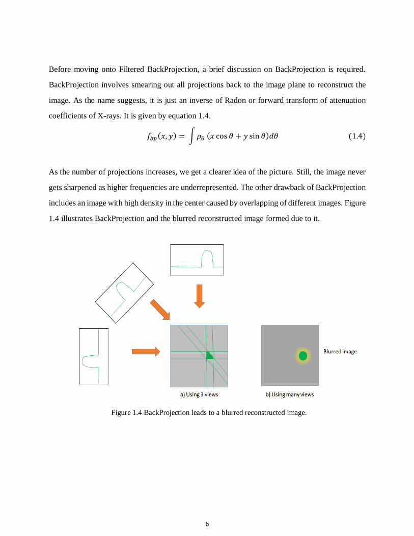
Before moving onto Filtered BackProjection, a brief discussion on BackProjection is required.

BackProjection involves smearing out all projections back to the image plane to reconstruct the

image. As the name suggests, it is just an inverse of Radon or forward transform of attenuation

coefficients of X-rays. It is given by equation 1.4.

𝑓𝑏𝑝(𝑥, 𝑦) = ∫ 𝜌𝜃 (𝑥 cos 𝜃 + 𝑦 sin 𝜃)𝑑𝜃 (1.4)

As the number of projections increases, we get a clearer idea of the picture. Still, the image never

gets sharpened as higher frequencies are underrepresented. The other drawback of BackProjection

includes an image with high density in the center caused by overlapping of different images. Figure

1.4 illustrates BackProjection and the blurred reconstructed image formed due to it.

Figure 1.4 BackProjection leads to a blurred reconstructed image.

7

1.4 Filtered BackProjection (FBP)

Filtered BackProjection is a combination of BackProjection and ramp filtering. FBP involves fast

Fourier transform, Ram-Lak filtering, and inverse Fourier transform. Figure 1.5 explains how FBP

can sharpen the reconstructed image.

Figure 1.5 Filtered BackProjection with the sharp reconstructed image.

It can be expressed as follows:

𝑔(𝑟, 𝜃) = ∫ ∫ [ ∫ 𝑓(𝜉, 𝜙)𝑒−𝑖2𝜋𝜌𝜉𝑑𝜉

∞

−∞

] |𝜌|𝑒𝑖2𝜋𝜌𝑟 cos(𝜃−𝜙)𝑑𝜌𝑑𝜙 (1.5)

∞

−∞

𝜋

0

where 𝑔(𝑟, 𝜃) is the reconstructed image, 𝑓(𝜉, 𝜙) are the original projections, and |𝜌| is the ramp

filtering function.

Fourier tranform of projections

Inverse Fourier transform

8

In equation 1.5 |𝜌| is the Ram-Lak filter which can be represented as:

𝐻𝑅𝐿(𝜔) = {|𝜔|, |𝜔| ≤ 2𝜋𝐵0, 𝑜𝑡ℎ𝑒𝑟𝑤𝑖𝑠𝑒

(1.6)

Figure 1.6 The frequency spectrum of Ram-Lak filter.

The steps involved in FBP are:

1. Take the Fourier transform for every projection.

2. Multiply with Ramp filter (Ram-Lak filter).

3. Take the inverse Fourier transform.

4. BackProject the filtered projections and integrate.

1.4 Sparse CT Reconstruction Literature Low-dose CT has been addressed in two ways. One way is to optimize the scanning setup for tube

voltage or current [1], [2]. The other way requires processing a smaller number of measurements

as if the X-ray source is turned on and off frequently. The process is known as sparse data

sampling. The reconstructed image suffers quality losses if directly fed to the reconstruction

algorithm. Thus, missing sparse data has to be generated [3] effectively.

Missing angle sinogram has been synthesized using linear interpolation or nearest-neighbor

interpolation. Such interpolation is essential as the artifacts are more pronounced after FBP in

9

reconstructed images. However, these conventional interpolation techniques are not useful when

the amount of sparsity goes on increasing. Recently, deep learning has been successfully used in

numerous computer vision applications[4]. Convolutional neural networks [5] [6] [7] have also

been very useful with the sparse-view CT problem. Similarly, generative adversarial networks [8,

9] were utilized for inpainting the sinogram. One of the important development has been an end-

to-end machine learning framework [10-13] but generalization of such models for each applicable

cases is something remains to be proved. There are other methods which try to address the angular

resolution issue [14, 15].

U-Net has been applied successfully in biomedical image segmentation [11, 16]. Another such

methodology [7] inspired Cho et al. to apply in the sinogram domain [17, 18] on simulated data.

However, so far most of those sinogram inpainting hypotheses for sparse-view CT have been only

trained and tested with simulated sinogram data, and comparisons for the performance of those

methods were mostly carried in the image domain rather than the sinogram domain, presumably

due to the lack of the experimental sinogram as ground truth. Experimental data which is super

sparsely sampled is a novel challenge addressed by this research. The novelty of current research

lies in the fact that the sinogram completion problem has been addressed in the projection domain

itself.

1.5 Organization of Thesis

The first chapter introduces CT and the ill-posed inverse problem in reconstruction. The central

slice theorem has been explained before the discussion on BackProjection. BackProjection is

followed by the explanation on the analytical method Filtered BackProjection in details. The

chapter also lists the attempts that have been made to address this issue. The various approaches,

along with merits and limitations, have been briefly discussed. The second chapter explains the

deep learning model. There is also a description of the training and testing methodology. The

implementation details of the experiment are listed in the last section. The third chapter provides

10

the results of the model using various performance metrics. The results have been compared in the

sinogram as well as in the image domain. The chapter also summarizes the quantitative analysis

using various performance metrics in the sinogram as well as the image domain. Finally, the results

are discussed, and the future scope is addressed in chapters 4 and 5. Bibliography and Appendix

containing the list of publications can be found at the end of the thesis.

11

Chapter 2

METHODS AND EXPERIMENTS

2.1 Data Preprocessing

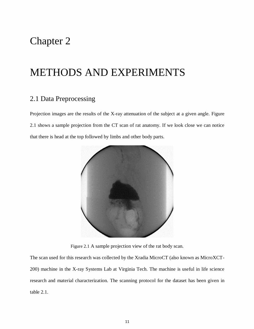
Projection images are the results of the X-ray attenuation of the subject at a given angle. Figure

2.1 shows a sample projection from the CT scan of rat anatomy. If we look close we can notice

that there is head at the top followed by limbs and other body parts.

Figure 2.1 A sample projection view of the rat body scan.

The scan used for this research was collected by the Xradia MicroCT (also known as MicroXCT-

200) machine in the X-ray Systems Lab at Virginia Tech. The machine is useful in life science

research and material characterization. The scanning protocol for the dataset has been given in

table 2.1.

12

Table 2.1 Scanning protocol for the CT scan.

Parameter Value

X-ray source 80 kV

Start angle -96 degree

End angle 96 degree

Number of projection images 1500

Binning 2

Source-sample distance 300 mm

Detector-sample distance 64.35 mm

While one scan can yield 1024 sinograms in total, only 625 sinograms in the central scans were

used in the study. The projection data was also cropped by cutting out 45 peripheral detector pixels

at each side. These pre-processing steps were applied to make sure all the collected sinograms are

in good quality. As per the Lambert-Beer law of attenuation, the received flux, 𝐼 is given by

𝐼 = 𝐼0𝑒𝑥𝑝 {− ∫ 𝜇(𝑥)𝑑𝑥𝐿

} (2.1)

where 𝐼0 is the incident flux and 𝜇(𝑥) is the absorption coefficient. Thus projection is given by:

− log (𝐼

𝐼0) = ∫ 𝜇(𝑥)𝑑𝑥

𝐿 (2.2)

The projection was log inverted with the blank image in each scan to get the actual attenuation, as

shown in equation 2.2. The sparse-view sinograms were constructed by selecting one projection

in every ten views to make the sparsity 90%. In contrast, the full-view sinograms were constructed

13

by using all the projections. As a result, each sparse-view sinogram is of size 150 × 935, and each

full-view sinogram is of size 1500 × 935. We interpolated the sparse-view sinogram to upscale its

size to be 1500 × 935 using linear interpolation. Then both interpolated sinograms and full-view

sinograms were divided into 64 × 64 patches so that they can be fed into the neural network. The

patch distribution is given in table 2.2.

Table 2.2 Distribution of patches for the model.

Number of Patches Percentage

Training 121680 65

Validation 18720 10

Testing 46800 25

Total 187200 100

2.2 The Residual U-Net Architecture

The U-Net proposed by Ronneberger [19] consists of a contracting arm at the left, followed by an

expansive arm. The network has proven capabilities in medical image segmentation. There is a

shortcut connection from input to output known as a residual connection. This connection helps

network understand the difference between the input and the output; hence, we get fast

convergence in training the model. Residual connections also play a pivotal role in avoiding the

vanishing gradient. It also helps in getting rid of streaking artifacts. Figure 2.2 shows the

architecture of the residual U-Net.

14

Figure 2.2 The architecture of residual U-Net.

The pooling layer in the U-Net has been replaced with a convolutional layer of size 2×2. Max

pooling is useful for downsampling and yielding the output quickly with fewer computations. It

involves picking up the max in a local neighborhood. As this network operates in the sinogram

domain, more weight needs to be given to the highly correlated pixels. The max values could be

ignored. Thus, restoration accuracy is maintained at the cost of computations. Patch-wise data were

fed to the network, so the RAM usage is limited. Thus, a general computer can also execute the

given algorithm.

The given architecture delivered most efficiently using four hidden layers. The other attempt

involved changing the number of layers, such as two, three, and five. The performance did not

improve by the addition or the deletion of layers. Each layer comprised of a combination of

convolutional blocks, a Rectified Linear Unit (ReLU), and a concatenation block. ReLU is a

popular activation function choice since it offers efficient gradient propagation. Output was a

simple mathematical addition with the input to facilitate residual connection.

15

2.3 Training

The interpolated sinogram was fed to the network, and output was compared with the

corresponding full-view sinogram. The network was trained to minimize the root-mean-square

error (RMSE) loss function between the input and the ground truth. Let 𝑁 denote the number of

batches, and let 𝑥 be the network output patch. The ground truth patch is denoted by 𝑦. For each

patch 𝑘, RMSE is given by:

𝑅𝑀𝑆𝐸 = 1

2𝑁∑ ‖𝑥𝑘 − 𝑦𝑘‖2

2𝑘 (2.3)

The learning rate was set to 0.0005 initially. It was decreased in the steps of 5% at every hundredth

epoch. Structural similarity (SSIM) was also plotted with respect to the ground truth. SSIM

captures correlation in the spatial neighborhood of a pixel. It is given by:

𝑆𝑆𝐼𝑀{𝑓1, 𝑓2} = 𝑆 = [2𝜇1𝜇2

𝜇12 + 𝜇2

2] × [2𝜎1𝜎2

𝜎12 + 𝜎2

2] × [𝜎12

𝜎1𝜎2] (2.4)

where 𝜇1, 𝜎1 is the average and variance of the image 𝑓1 and 𝜇2, 𝜎2 is the average and variance of

the image 𝑓2.

The evaluation metrics also Peak signal-to-noise ratio. PSNR is given by:

𝑃𝑆𝑁𝑅 = 20 × log10 (𝑀𝐴𝑋

𝑅𝑀𝑆𝐸) (2.5)

where MAX is the maximum possible pixel value of an image.

PSNR is widely used to measure reconstruction quality in compression as it approximates the

human perception of reconstruction.

From the input as well as ground truth patches of size 64×64 were extracted. The patch size of

48×48 was also tried, but it was not effective given the computing capabilities. Zero-padding was

used with stride as one while performing the convolution operations to match the matrix

16

dimensions. To utilize the full GPU processing capabilities, batch size of 400 was used. A single

batch comprised 25 columns and 12 rows each of patch size 64×64. The dataset was continuously

shuffled to avoid overfitting. It also helped in generalization and reducing the variance. The

training of around 5000 epochs was completed in five hours. Validation error was calculated at the

steps of 50 epochs. Validation error helped network tune hyperparameters of the hidden layers.

The other parameter that was monitored for training the model apart from RMSE was SSIM.

2.4 Implementation Details

Each projection had 1024×1024 pixels. Such 1500 projections were captured in the scan. Out of

these middle 625 sinograms were taken for processing. Each sinogram was cropped 45 pixels in

each side, resulting in size 1500×935. These steps were carried out to have better quality data.

Reference, interpolated sinograms were formed from the projection views by using each row of

the projection data. The training was done on a computer with Intel Core i5-7400 CPU and 16GB

RAM. Nvidia GTX Titan X GPU was utilized during the training process. The hyperparameters

were tuned in such a way that each epoch was completed in a few seconds. The convolution and

deconvolution kernels were initialized with random Gaussian distributions with 0 mean and 0.01

standard deviation. When the network was fully trained, it was tested with sparse-view sinograms

from the test dataset. The relation between the sparse-view sinogram, the interpolated input

sinogram, the deep learning-based corrected sinogram, and the full-view ground truth sonogram is

shown in figure 2.3. They are reconstructed using FBP.

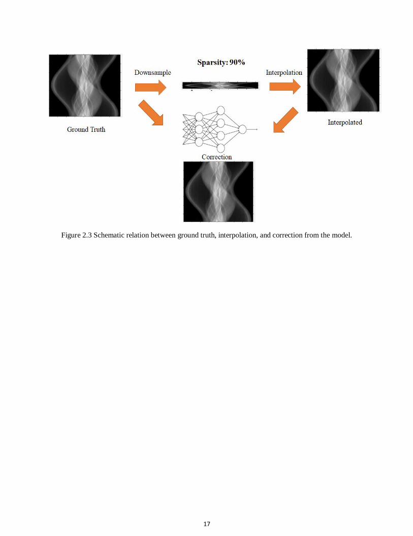
17

Figure 2.3 Schematic relation between ground truth, interpolation, and correction from the model.

18

Chapter 3

RESULTS

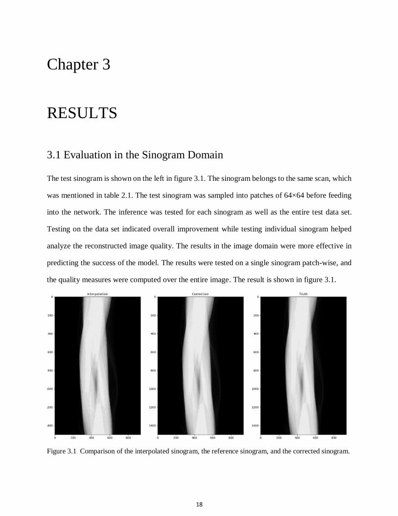
3.1 Evaluation in the Sinogram Domain

The test sinogram is shown on the left in figure 3.1. The sinogram belongs to the same scan, which

was mentioned in table 2.1. The test sinogram was sampled into patches of 64×64 before feeding

into the network. The inference was tested for each sinogram as well as the entire test data set.

Testing on the data set indicated overall improvement while testing individual sinogram helped

analyze the reconstructed image quality. The results in the image domain were more effective in

predicting the success of the model. The results were tested on a single sinogram patch-wise, and

the quality measures were computed over the entire image. The result is shown in figure 3.1.

Figure 3.1 Comparison of the interpolated sinogram, the reference sinogram, and the corrected sinogram.

19

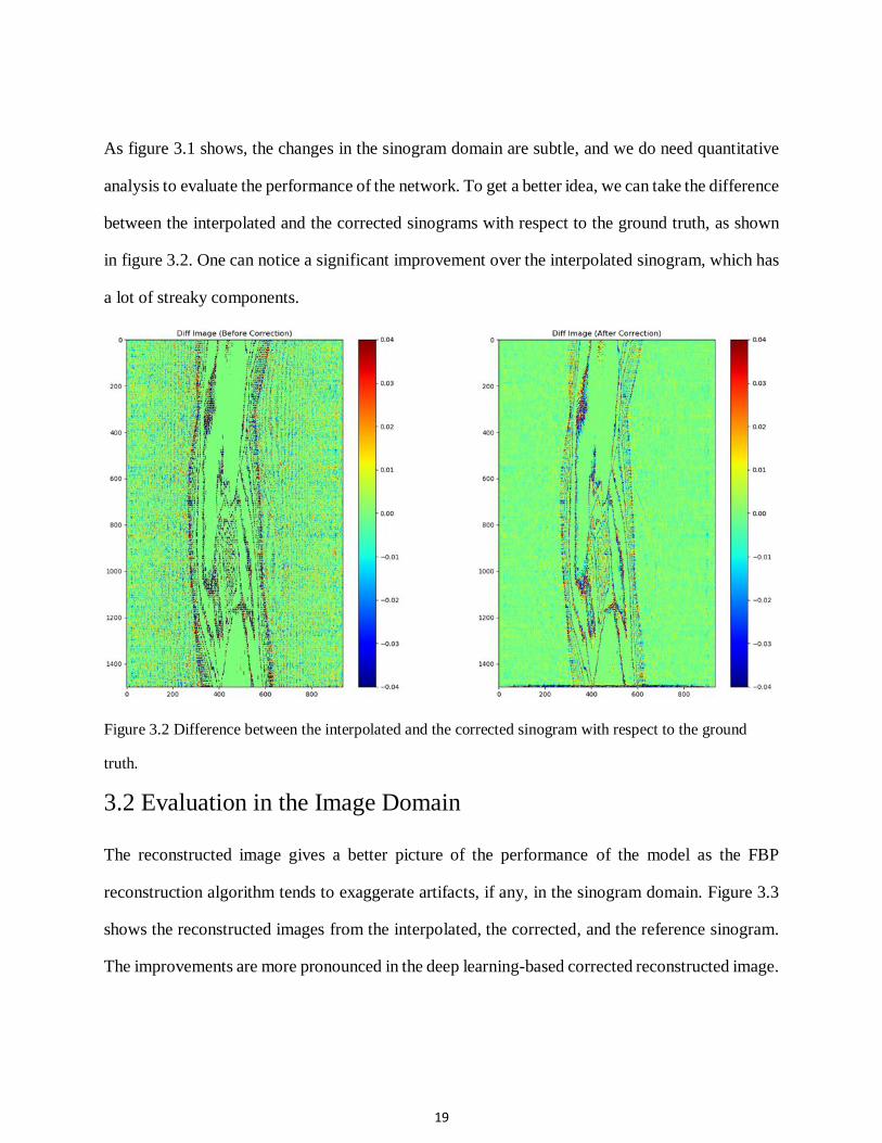
As figure 3.1 shows, the changes in the sinogram domain are subtle, and we do need quantitative

analysis to evaluate the performance of the network. To get a better idea, we can take the difference

between the interpolated and the corrected sinograms with respect to the ground truth, as shown

in figure 3.2. One can notice a significant improvement over the interpolated sinogram, which has

a lot of streaky components.

Figure 3.2 Difference between the interpolated and the corrected sinogram with respect to the ground

truth.

3.2 Evaluation in the Image Domain

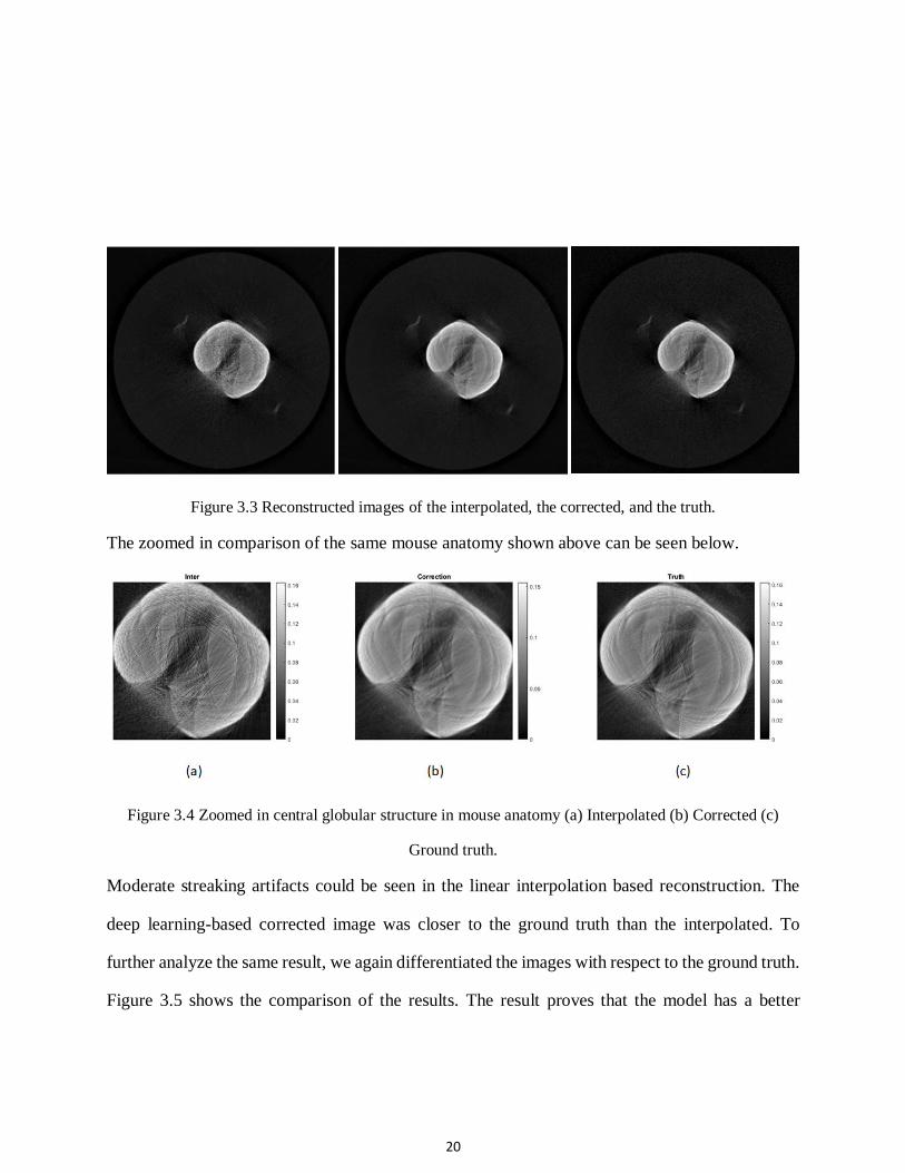
The reconstructed image gives a better picture of the performance of the model as the FBP

reconstruction algorithm tends to exaggerate artifacts, if any, in the sinogram domain. Figure 3.3

shows the reconstructed images from the interpolated, the corrected, and the reference sinogram.

The improvements are more pronounced in the deep learning-based corrected reconstructed image.

20

Figure 3.3 Reconstructed images of the interpolated, the corrected, and the truth.

The zoomed in comparison of the same mouse anatomy shown above can be seen below.

Figure 3.4 Zoomed in central globular structure in mouse anatomy (a) Interpolated (b) Corrected (c)

Ground truth.

Moderate streaking artifacts could be seen in the linear interpolation based reconstruction. The

deep learning-based corrected image was closer to the ground truth than the interpolated. To

further analyze the same result, we again differentiated the images with respect to the ground truth.

Figure 3.5 shows the comparison of the results. The result proves that the model has a better

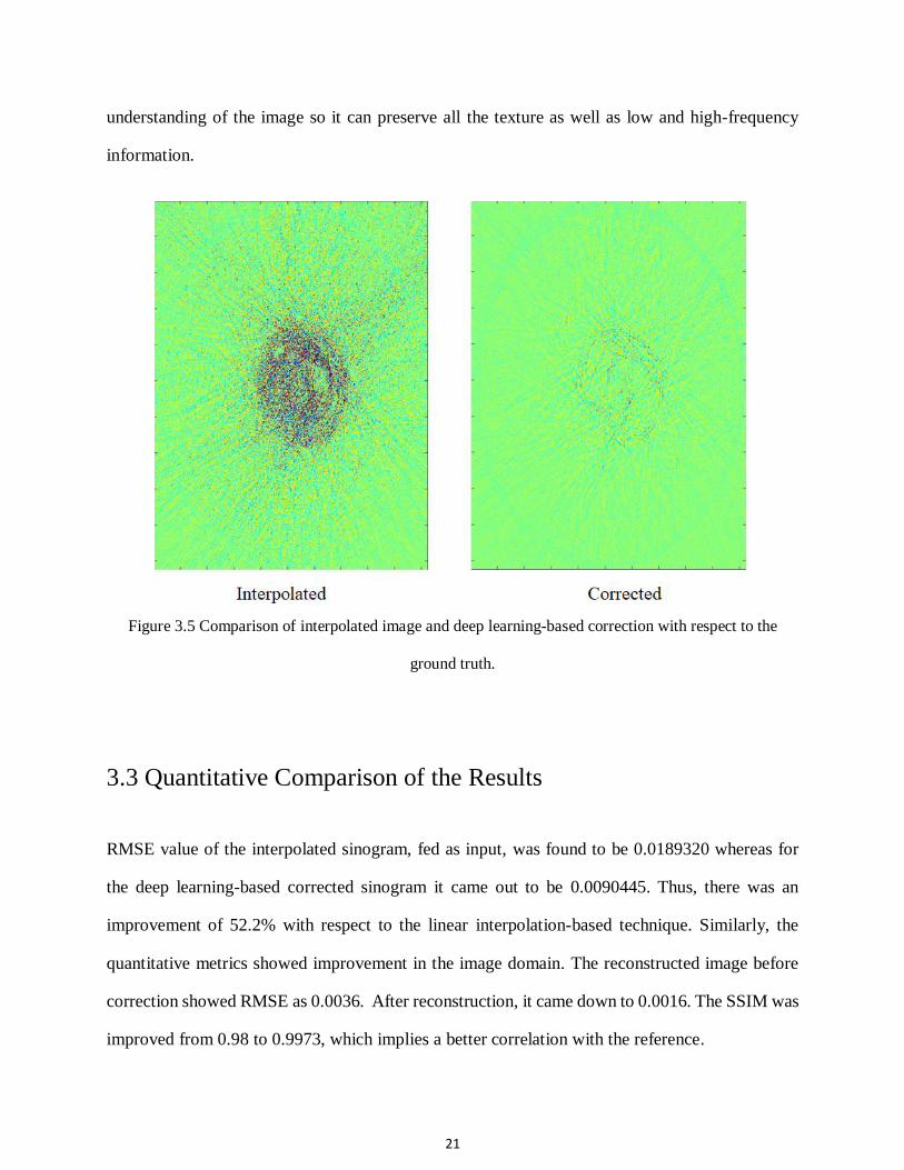
21

understanding of the image so it can preserve all the texture as well as low and high-frequency

information.

Figure 3.5 Comparison of interpolated image and deep learning-based correction with respect to the

ground truth.

3.3 Quantitative Comparison of the Results

RMSE value of the interpolated sinogram, fed as input, was found to be 0.0189320 whereas for

the deep learning-based corrected sinogram it came out to be 0.0090445. Thus, there was an

improvement of 52.2% with respect to the linear interpolation-based technique. Similarly, the

quantitative metrics showed improvement in the image domain. The reconstructed image before

correction showed RMSE as 0.0036. After reconstruction, it came down to 0.0016. The SSIM was

improved from 0.98 to 0.9973, which implies a better correlation with the reference.

22

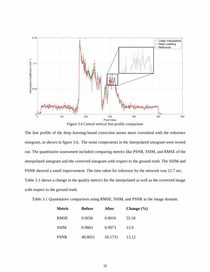
Figure 3.6 Central vertical line profile comparison

The line profile of the deep learning-based correction seems more correlated with the reference

sinogram, as shown in figure 3.6. The noise components in the interpolated sinogram were ironed

out. The quantitative assessment included comparing metrics like PSNR, SSIM, and RMSE of the

interpolated sinogram and the corrected sinogram with respect to the ground truth. The SSIM and

PSNR showed a small improvement. The time taken for inference by the network was 12.7 sec.

Table 3.1 shows a change in the quality metrics for the interpolated as well as the corrected image

with respect to the ground truth.

Table 3.1 Quantitative comparison using RMSE, SSIM, and PSNR in the image domain.

Metric Before After Change (%)

RMSE 0.0036 0.0016 55.56

SSIM 0.9863 0.9973 13.9

PSNR 48.8051 56.1731 13.12

23

In this table, the column marked as before indicates the interpolated sinogram with respect to the

ground truth while after represents corrected sinogram with respect to the ground truth. Inference

for the entire test dataset (46800 patches) took 144.67 sec. These are random patches and therefore,

not be reconstructed. There was an improvement of around 81%, as shown in table 3.2.

Table 3.2 Quantitative comparison of RMSE for the entire test dataset in the sinogram domain.

Metric Before After Change (%)

RMSE 0.0062209 0.0011503 81.5

24

Chapter 4

DISCUSSION AND CONCLUSIONS

U-Net has proven capabilities in image segmentation. In this thesis, the residual U-Net has been

evaluated for the interpolating missing data in the sparse-view sinogram. The results are promising

for the scans of the same type. Though the generalization capabilities of the network are limited,

the results do encourage further investigation.

The other architectures like Autoencoder and Convolutional Neural Network with up to eighteen

hidden layers were tried but, the results were not promising. The U-Net model was also modified

by adding the batch normalization layers, but the performance degraded presumably because of

the nature of experimental data. The pooling layers were not used because the sinogram is too

sensitive to such processing and computing capabilities of the GPU were available at our disposal.

The proposed method was effective in interpolating missing CT data. The loss function helped

minimize the l2-norm and fetched improvement in the other quality metrics. There remains scope

to explore loss function that is more tuned to image perceptual quality.

The baseline used for the model was constructed using linear interpolation. An improvement

suggested by the committee includes a stronger baseline which takes into consideration the angular

nature of sinogram.

25

Chapter 5

FUTURE DIRECTIONS

In this research project, a novel deep learning-based method has been proposed for sparse-view

CT. As the graphics processing hardware of modern computers tends to become more and more

sophisticated, the complexity of the neural network model that could be run also knows no bounds.

Still, taking into consideration the need for real-time diagnosis, we have proposed a solution which

operates in the sinogram domain. Future work might involve generative adversarial network based

deep learning model. In that, PatchGAN promises significant improvement over the conventional.

Deep learning is a cutting edge field, and there are new models proposed now and then. New

frontiers [21, 22] are being explored and put to use for various real-life application. Therefore, the

possibilities are endless.

26

BIBLIOGRAPHY

[1] L. Yu, X. Liu, S. Leng, J. M. Kofler, J. C. Ramirez-Giraldo, M. Qu, J. Christner, J. G.

Fletcher, and C. H. McCollough, “Radiation dose reduction in computed tomography:

techniques and future perspective,” Imaging in Medicine, 1(1), 65 (2009).

[2] Q. Xu, H. Yu, J. Bennett, P. He, R. Zainon, R. Doesburg, A. Opie, M. Walsh, H. Shen, A.

Butler, P. Butler, X. Mou, and G. Wang, “Image reconstruction for hybrid true-color micro-

CT,” IEEE Trans Biomed Eng, 59(6), 1711-9 (2012).

[3] S. Abbas, J. Min, and S. Cho, “Super-sparsely view-sampled cone-beam CT by

incorporating prior data,” Journal of X-ray science and technology, 21(1), 71-83 (2013).

[4] L. A. Gatys, A. S. Ecker, and M. Bethge, "Image style transfer using convolutional neural

networks,"Proceedings of the IEEE Conference on Computer Vision and Pattern

Recognition. 2414-2423.

[5] Z. Zhang, X. Liang, X. Dong, Y. Xie, and G. Cao, “A Sparse-View CT Reconstruction

Method Based on Combination of DenseNet and Deconvolution.”

[6] Y. Han, J. Yoo, and J. C. Ye, “Deep residual learning for compressed sensing CT

reconstruction via persistent homology analysis,” arXiv preprint arXiv:1611.06391,

(2016).

27

[7] K. H. Jin, M. T. McCann, E. Froustey, and M. Unser, “Deep convolutional neural network

for inverse problems in imaging,” IEEE Transactions on Image Processing, 26(9), 4509-

4522 (2017).

[8] R. Anirudh, H. Kim, J. J. Thiagarajan, K. Aditya Mohan, K. Champley, and T. Bremer,

"Lose the views: Limited angle CT reconstruction via implicit sinogram

completion,"Proceedings of the IEEE Conference on Computer Vision and Pattern

Recognition. 6343-6352.

[9] X. Yi, and P. Babyn, “Sharpness-aware low-dose CT denoising using conditional

generative adversarial network,” Journal of digital imaging, 1-15 (2018).

[10] T. Würfl, M. Hoffmann, V. Christlein, K. Breininger, Y. Huang, M. Unberath, and A. K.

Maier, “Deep learning computed tomography: Learning projection-domain weights from

image domain in limited angle problems,” IEEE transactions on medical imaging, 37(6),

1454-1463 (2018).

[11] H. Yuan, J. Jia, and Z. Zhu, "SIPID: A deep learning framework for sinogram interpolation

and image denoising in low-dose CT reconstruction,"Biomedical Imaging (ISBI 2018),

2018 IEEE 15th International Symposium on. 1521-1524.

[12] B. Zhu, J. Z. Liu, S. F. Cauley, B. R. Rosen, and M. S. Rosen, “Image reconstruction by

domain-transform manifold learning,” Nature, 555(7697), 487 (2018).

[13] J. Rick Chang, C.-L. Li, B. Poczos, B. Vijaya Kumar, and A. C. Sankaranarayanan, "One

Network to Solve Them All--Solving Linear Inverse Problems Using Deep Projection

Models,"Proceedings of the IEEE International Conference on Computer Vision. 5888-

5897.

28

[14] K. Liang, H. Yang, K. Kang, and Y. Xing, "Improve angular resolution for sparse-view CT

with residual convolutional neural network,"Medical Imaging 2018: Physics of Medical

Imaging. ^10573, 105731K.

[15] M. Bertram, J. Wiegert, D. Schafer, T. Aach, and G. Rose, “Directional view interpolation

for compensation of sparse angular sampling in cone-beam CT,” IEEE transactions on

medical imaging, 28(7), 1011-1022 (2009).

[16] O. Ronneberger, P. Fischer, and T. Brox, "U-net: Convolutional networks for biomedical

image segmentation,"International Conference on Medical image computing and

computer-assisted intervention. 234-241.

[17] H. Lee, J. Lee, and S. Cho, "View-interpolation of sparsely sampled sinogram using

convolutional neural network,"Medical Imaging 2017: Image Processing. ^10133,

1013328.

[18] J. Lee, H. Lee, and S. Cho, "Sinogram synthesis using convolutional-neural-network for

sparsely view-sampled CT,"Medical Imaging 2018: Image Processing. ^10574, 105742A.

[19] A. Radford, L. Metz, and S. Chintala, "Unsupervised representation learning with deep

convolutional generative adversarial networks," arXiv preprint arXiv: 1511.06434, 2015.

[20] M. U. Ghani and W. C. Karl, "Deep Learning-Based Sinogram Completion for Low-Dose

CT," in 2018 IEEE 13th Image, Video, and Multidimensional Signal Processing Workshop

(IVMSP), 2018, pp. 1-5: IEEE

[21] M. M. Bronstein, J. Bruna, Y. LeCun, A. Szlam, and P. Vandergheynst. Geometric deep

learning: Going beyond euclidean data. IEEE Signal Processing Magazine, 34(4):18–42,

2017.

29

[22] Xing Lin, Yair Rivenson, Nezih T. Yardimci, Muhammed Veli, Yi Luo, Mona Jarrahi, and

Aydogan Ozcan. All-optical machine learning using diffractive deep neural networks.

Science, 2018.

Appendix A

PUBLICATION INFORMATION

1. Z. Zhang, X. Dong, S. Vekhande, and G. Cao, “A Deep Learning Based Reconstruction

Method for Sparse-view CT, ” 40th International Conference of the IEEE Engineering in

Medicine and Biology Conference (EMBC), 2018.

2. X. Dong, S. Vekhande, and G. Cao, “Sinogram interpolation for sparse-view micro-CT

with deep learning neural network,” International Society for Optics and Photonics (SPIE)

Medical Imaging conference, 2019

3. Z. Zhang, X. Dong, S. Vekhande, and G. Cao “Deep Learning Based Reconstruction

Method for Sparse-View CT,” 2019 IEEE 16th International Symposium on Biomedical

Imaging (ISBI)