Embed Size (px)
Citation preview

1
Deep Learning of Part-based Representation of DataUsing Sparse Autoencoders with Nonnegativity
ConstraintsEhsan Hosseini-Asl, Member, IEEE, Jacek M. Zurada, Life Fellow, IEEE, Olfa Nasraoui, Senior Member, IEEE
Abstract—We demonstrate a new deep learning autoen-coder network, trained by a nonnegativity constraint algorithm(NCAE), that learns features which show part-based represen-tation of data. The learning algorithm is based on constrainingnegative weights. The performance of the algorithm is assessedbased on decomposing data into parts and its prediction per-formance is tested on three standard image data sets andone text dataset. The results indicate that the nonnegativityconstraint forces the autoencoder to learn features that amountto a part-based representation of data, while improving sparsityand reconstruction quality in comparison with the traditionalsparse autoencoder and Nonnegative Matrix Factorization. It isalso shown that this newly acquired representation improves theprediction performance of a deep neural network.
Index Terms—Autoencoder, feature learning, nonnegativityconstraints, deep architectures, part-based representation.
I. INTRODUCTION
RECENT studies have shown that deep architectures arecapable of learning complex data distributions while
achieving good generalization performance and efficient rep-resentation of patterns in challenging recognition tasks [1],[2], [3], [4], [5], [6]. Deep architecture networks have manylevels of nonlinearities, giving them an ability to compactlyrepresent highly nonlinear complex mappings. However, theyare difficult to train, since there are many hidden layers withmany connections, which causes gradient-based optimizationwith random initialization to get stuck in poor solutions [7].To improve on this bottleneck, a greedy layer-wise trainingalgorithm was proposed in [8], where each layer is separatelyinitialized by unsupervised pre-training, then the stacked layersare fine-tuned using a supervised learning algorithm [3], [7].It was shown that an unsupervised pre-training phase of eachlayer helps in capturing the patterns in high-dimensional data,which results in a better representation in a low-dimensionalencoding space [3], and could result in more sparse featurelearning [9]. This pre-training also improves the supervisedfine-tuning algorithm for classification by guiding the learningalgorithm towards local minima of the error function, thatsupport better generalization on training data [10], [11].
E. Hosseini-Asl is with the Department of Electrical and Computer Engi-neering, University of Louisville, Louisville, KY, 40292 USA. (Correspondingauthor, e-mail: [email protected]).
J. M. Zurada is with the Department of Electrical and Computer Engineer-ing, University of Louisville, Louisville, KY, 40292 USA, and also with theInformation Technology Institute, University of Social Science,Łodz 90-113,Poland (e-mail: [email protected]).
O. Nasraoui is with the Department of Computer Science, University ofLouisville, Louisville, KY, 40292 USA. (e-mail: [email protected]).
There are two popular algorithms for unsupervised learningwhich have been shown to work well for producing a goodrepresentation for initializing deep structures [12]: RestrictedBoltzmann Machines (RBMs), trained with contrastive diver-gence [13], and different types of autoencoders [2]. In thispaper, we focus on unsupervised feature learning based onautoencoders.
Autoencoder neural networks are trained with an unsuper-vised learning algorithm based on reconstructing the inputfrom its encoded representation, while constraining the rep-resentation to have some desirable properties. Deep networksbased on autoencoders are created by stacking pre-trainedautoencoders layer by layer, followed by a supervised fine-tuning algorithm [7]. As discussed before, a key contributor tosuccessful training of a deep network is a proper initializationof the layers based on a local unsupervised criterion [12].In the case of autoencoders, the reconstruction error is usedas a local criterion for unsupervised learning of each layer.Each layer produces a representation of its input at the hiddenlayer, where this representation is used as the input to the nextlayer. Therefore, a learning algorithm which results in lowerreconstruction error at each layer should create a more accuraterepresentation of data, and deliver a better initialization oflayer parameters; This, in turn, improves the deep network’sprediction performance [12]. One additional criterion proposedfor this model is sparsity of the autoencoding. Sparsenessof the representation, i.e. activity of hidden nodes, has beenshown to have some advantages in robustness to noise andimproved classification in high-dimensional spaces [9], [14].
This paper demonstrates how to achieve a meaningfulrepresentation from data that discovers the hidden structureof high-dimensional data based on autoencoders [15]. It hasbeen shown that data is represented in hierarchical layersthrough the visual cortex [16], where some psychological andphysiological evidence showed that data is represented by part-based decomposition in the human brain [17]. Inspired bythe idea of sparse coding [18], [19], [20] and NonnegativeMatrix Factorization (NMF) [21], [22], learning features thatexhibit sparse part-based representation of data (decomposingdata into parts) is expected to disentangle the hidden structureof data. We develop a deep network by extracting part-based features in hierarchical layers, and show that thesefeatures result in good generalization ability for the trainedmodel, and improve the reconstruction error. Using NMF, thefeatures and the encoding of data are forced to be nonnegative,which results in part-based additive representation of data.

2
However, while sparse coding within NMF needs an expensiveoptimization process to find the encoding of test data, thisprocess is very fast in autoencoders [9]. Therefore, trainingan autoencoder which could exploit the benefits of part-basedrepresentation using nonnegativity is expected to improve theperformance of a deep learning network.
The most closely related work to ours is that of Lemmeet al. on the Nonnegative Sparse Autoencoder (NNSAE)[23].In their approach, an online training algorithm has beendeveloped for an autoencoder with tied weights, and a linearfunction at the output layer of the autoencoder to simplifythe training algorithm. The key difference compared to ournetwork is that we use a general autoencoder with trainableweights for both the hidden and the output layers. We alsouse a nonlinear function for the nodes in each layer whichmakes our model more flexible. The other related work isby Chorowski et al. [24], who demonstrated that a multilayerperceptron network with softmax output nodes trained withnonnegative weights, was capable of extracting understandablelatent features, which consist of part-based representation ofdata. It was illustrated with extracting characteristic parts ofhandwritten digits and extracting semantic features from data.However, the improved transparency had slightly reduced thenetwork’s prediction performance. Moreover, it is difficult toapply the method to train a large deep network with severallayers. The reason is that random initialization of the networkwas used instead of pretraining with the greedy layer-wisealgorithm [24]. In contrast, our method for pretraining andfine-tuning of a deep network can be easily scaled up to largedeep networks, since it uses greedy layer-wise pretraining.Another related work is by Nguyen et al. [25], with thenonnegativity constraint applied to train an RBM network(NRBM). It possesses a certain similarity to RBM and NMF interms of part-based representation and classification accuracy.However, RBM uses a stochastic approach based on maxi-mizing the joint probability between the visible and hiddenunits, whereas the autoencoder uses a deterministic approachbased on minimizing the reconstruction error. In this case,part-whole decomposition of data based on additive parts canbe easily translated by incorporating nonnegative weights inthe encoding and decoding layers of the autoencoder, whichtries to minimize the reconstruction error. Therefore, we usean autoencoder instead of RBM to produce a part-basedrepresentation of data.
In this paper, we propose a new approach to train anautoencoder by introducing a nonnegativity constraint intoits learning to learn a sparse, part-based representation ofdata. The training is then extended to train a deep networkwith stacked autoencoders and a softmax classification layer,while again constraining the weights of the network to benonnegative. Our goal is two-fold: part-based representation inthe autoencoder network to improve its ability to disentanglethe hidden structure of the data, and producing a better recon-struction of the data. We also show that these criteria improvethe prediction performance of a deep learning network.
The performance of our method is first compared withSparse Autoencoder (SAE) [26], Nonnegative Sparse Autoen-coder (NNSAE) [23], and NMF [27] in terms of extracting
latent features, reconstruction error and sparsity of representa-tion on several image and text benchmark datasets. Then theclassification performance of our deep learning approach isshown to significantly outperform the related deep networksreported in the literature based on SAE, NNSAE, DenoisingAutoencoder (DAE) [12], and Dropout Autoencoder (DpAE)[28].
II. METHODS
As mentioned, an autoencoder neural network tries to re-construct its input vector at the output through unsupervisedlearning [12], [29]. As shown in Fig. 1(a), it tries to learn afunction,
ˆx = fW,b(x) ⇡ x (1)
where x is the input vector, while W = {W1,W2} andb = {b1, b2} represent weights and biases of both layers,respectively. It takes an input vector x 2 [0, 1]
n, and first mapsit to a hidden representation through a deterministic mapping,parametrized by ✓1 = {W1, b1}, and given by
h = g
✓1(x) = � (W1x + b1) (2)
where h 2 [0, 1]
n
0, W1 2 R
n
0⇥n, b 2 R
n
0⇥1, and �(x)
denotes an element-wise application of the logistic sigmoid,�(x) =
1/(1 + exp(�x)). The resulting hidden representation, h,
is then mapped back to a reconstructed vector, ˆx 2 [0, 1]
n, bya similar mapping function, parametrized by ✓2 = {W2, b2},
ˆx = g
✓2(h) = � (W2h + b2) (3)
where W2 2 R
n⇥n
0and b2 2 R
n⇥1. To optimize theparameters of the model in Eq. (1), i.e. ✓ = {✓1, ✓2}, theaverage reconstruction error is used as the cost function,
JE(W, b) = 1
m
mX
r=1
1
2
k ˆx(r) � x(r) k2 (4)
where m is the number of training samples.By imposing meaningful limitations on parameters ✓, e.g.
limiting the dimension n
0 of the hidden representation h, theautoencoder learns a compressed representation of the input,which helps discover the latent structure of data in a high-dimensional space.
Sparse representation can provide a simple interpretation ofthe input data in terms of a reduced number of parts and byextracting the structure hidden in the data. Several algorithmswere proposed to learn a sparse representation using autoen-coders [8], [19]. One common method for imposing sparsityis to limit the activation of hidden units h using the Kullback-Leibler (KL) divergence function [14], [30]. Let h
j
�x(r)
�
denote the activation of hidden unit j with respect to the inputx(r). Then the average activation of this hidden unit is:
p
j
=
1
m
mX
r=1
h
j
(x(r)) (5)
To enforce sparsity, we constrain the average activation p
j
= p,where p is the sparsity parameter chosen to be a small positivenumber near 0. This also relates to the normalization of theinput to the neurons of the next layer which results in faster

3
(a) (b)
Fig. 1. (a) Schematic diagram of (a) a three-layer autoencoder and (b) a deep network
convergence of training using the backpropagation algorithm[31]. To use this constraint in Eq. (4), we try to minimize theKL divergence similarity between p
j
and p,
JKL(p k ˆp) =n
0X
j=1
p log
p
p
j
+ (1� p) log
1� p
1� p
j
(6)
where ˆp is the vector of average hidden activities. To preventoverfitting, a weight decay term is also added to the costfunction of Eq. (4) [32]. The final cost function for learninga Sparse Autoencoder (SAE) becomes as follows:
JSAE(W, b) = JE(W, b) + �JKL(p k ˆp)
+
�
2
2X
l=1
slX
i=1
sl+1X
j=1
⇣w
(l)ij
⌘2 (7)
where � controls the sparsity penalty term, � controls thepenalty term facilitating weight decay, and s
l
and s
l+1 arethe sizes of adjacent layers.
A. Part-based Representation Using a Nonnegativity Con-
strained Autoencoder (NCAE)
Ideally, part-based representation is implemented throughdecomposing data into parts, which when combined, producethe original data. However, the combination of parts hereis only allowed to be additive [22]. As shown in [24] thatdemonstrates part-based representation, the input data can bedecomposed in each layer into parts, while the weights in Ware constrained to be nonnegative [24].
Intuitively, to improve the performance of the autoencoderin terms of reconstruction of input data, it should be able todecompose data into parts which are sparse in the encodinglayer and then combine them in an additive manner in thedecoding layer. To achieve this goal, a nonnegativity constraintis imposed on the connecting weights W. This means that thecolumn vectors of W are coerced to be sparse, i.e. only afraction of entries per column should remain non-zero.
To encourage nonnegativity in W, the weight decay term inEq. (7) is replaced and a quadratic function [33], [25] is used.This results in the following cost function for NCAE:
JNCAE (W, b) = JE (W, b) + �JKL(p k ˆp)
+
↵
2
2X
l=1
slX
i=1
sl+1X
j=1
f
⇣w
(l)ij
⌘ (8)
where
f(w
ij
) =
⇢w
2ij
w
ij
< 0
0 w
ij
� 0
(9)
and ↵ � 0. Minimization of Eq. (8) would result in reducingthe average reconstruction error, increased sparsity of hiddenlayer activations, and reduced number of nonnegative weightsof each layer.
To update the weights and biases, we compute the gradientof Eq. (8) used in the backpropagation algorithm:
w
(l)ij
= w
(l)ij
� ⌘
@
@w
(l)ij
JNCAE(W, b) (10)
b
(l)i
= b
(l)i
� ⌘
@
@b
(l)i
JNCAE(W, b) (11)
where ⌘ > 0 is the learning rate. The derivative of Eq. (8)with respect to the weights consists of three terms as shownbelow,
@
@w
(l)ij
JNCAE(W, b) = @
@w
(l)ij
JE (W, b)
+ �
@
@w
(l)ij
JKL (p k ˆp)
+ ↵g
⇣w
(l)ij
⌘
(12)
where
g(x) =
⇢w
ij
w
ij
< 0
0 w
ij
� 0
(13)
The derivative term in Eq. (11) and the first two terms in Eq.(12) are computed using the backpropagation algorithm [26],[34].
4
(a) SAE
(b) NNSAE
(c) NCAE*
(d) NMF
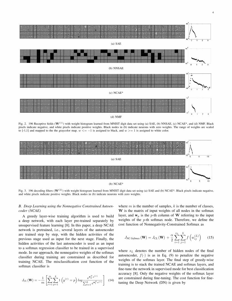
Fig. 2. 196 Receptive fields (W(1)) with weight histogram learned from MNIST digit data set using (a) SAE, (b) NNSAE, (c) NCAE*, and (d) NMF. Blackpixels indicate negative, and white pixels indicate positive weights. Black nodes in (b) indicate neurons with zero weights. The range of weights are scaledto [-1,1] and mapped to the the graycolor map. w <= �1 is assigned to black, and w >= 1 is assigned to white color.
(a) SAE
(b) NCAE*
Fig. 3. 196 decoding filters (W(2)) with weight histogram learned from MNIST digit data set using (a) SAE and (b) NCAE*. Black pixels indicate negative,and white pixels indicate positive weights. Black nodes in (b) indicate neurons with zero weights.
B. Deep Learning using the Nonnegative Constrained Autoen-
coder (NCAE)
A greedy layer-wise training algorithm is used to builda deep network, with each layer pre-trained separately byunsupervised feature learning [8]. In this paper, a deep NCAEnetwork is pretrained, i.e., several layers of the autoencoderare trained step by step, with the hidden activities of theprevious stage used as input for the next stage. Finally, thehidden activities of the last autoencoder is used as an inputto a softmax regression classifier to be trained in a supervisedmode. In our approach, the nonnegative weights of the softmaxclassifier during training are constrained as described fortraining NCAE. The misclassification cost function of thesoftmax classifier is
J
CL
(W) = � 1m
"mX
r=1
kX
p=1
1⇣y
(r) = p
⌘log
e
wTp x
(r)
Pk
l=1 ewTl x
(r)
#(14)
where m is the number of samples, k is the number of classes,W is the matrix of input weights of all nodes in the softmaxlayer, and w
p
is the p-th column of W referring to the inputweights of the p-th softmax node. Therefore, we define thecost function of Nonnegativity-Constrained Softmax as
J
NC-Softmax
(W) = J
CL
(W) +
↵
2
sLX
i=1
kX
j=1
f
⇣w
(L)ij
⌘(15)
where s
L
denotes the number of hidden nodes of the finalautoencoder, f(·) is as in Eq. (9) to penalize the negativeweights of the softmax layer. The final step of greedy-wisetraining is to stack the trained NCAE and softmax layers, andfine-tune the network in supervised mode for best classificationaccuracy [8]. Only the negative weights of the softmax layerare constrained during fine-tuning. The cost function for fine-tuning the Deep Network (DN) is given by

5
J
DN
(W, b) = J
CL
(WDN
, bDN
) +
↵
2
sLX
i=1
kX
j=1
f
⇣w
(L)ij
⌘(16)
where WDN
contains the input weights of the NCAE andsoftmax layers, and b
DN
is the bias input of NCAE layers, asshown in Fig. 1(b).
A batch gradient descent algorithm is used, where theLimited-memory BFGS (L-BFGS) quasi-Newton method [35]is employed for minimization of Eq. (8), Eq. (15), and Eq.(16). The L-BFGS algorithm computes an approximation ofthe inverse of the Hessian matrix, which results in less memoryto store the vectors which approximate the Hessian matrix. Thedetails of the algorithm and the software implementation canbe found in [36].
III. EXPERIMENTAL RESULTS
This section reports the performance tests of the proposedmethod in unsupervised feature learning for three benchmarkimage data sets and one text dataset. A deep network usingNCAE as a building block is trained, and its classificationperformance is evaluated. We use the MNIST digit dataset for handwritten digits [37], the ORL face data set [38]for face images, and the small NORB object recognitiondataset [39]. The Reuters 21578 document corpus is alsoused to evaluate the ability of the proposed method inlearning semantic features. The Matlab implementationof the NCAE algorithm can be downloaded fromhttps://github.com/ehosseiniasl/Nonnegativity-Constrained-Autoencoder-NCAE.githttps://github.com/ehosseiniasl/Nonnegativity-Constrained-Autoencoder-NCAE.git.
TABLE IPARAMETER SETTINGS OF EACH ALGORITHM
Parameters SAE NCAE* NMFSparsity penalty (�) 3 3 -
Sparsity parameter (p) 0.05 0.05 -Weight decay penalty (�) 0.003 - -
Nonnegativity constraint penalty (↵) - 0.003 -Convergence Tolerance 1e-9 1e-9 1e-9
Maximum No. of Iterations 400 400 400
A. Unsupervised Feature Learning
A three-layer NCAE network using Eq.(8) was trained. Inthe case of image data, the input weights of hidden nodesW1 are rendered as images called receptive fields. The resultsof the NCAE method are compared to the receptive fieldslearned by a three-layer Sparse Autoencoder (SAE) of Eq.(7), Nonnegative Sparse Autoencoder (NNSAE) [23], and thebasis images learned by NMF. The multiplicative algorithmhas been used to compute the basis images W of NMF [22].In the case of text data, W1 represents the group of words toevaluate the ability to extract meaningful features connectedto the topics in the document corpus.
To tune the hyperparameters, each algorithm has been testedwith a range of values for each regularization parameter tominimize the cost in Eq. (4) and Eq. (8). The value for
0 0.2 0.4 0.6 0.8 10
20
40
SAE
0 0.2 0.4 0.6 0.8 10
20
40
NNSAE
0 0.2 0.4 0.6 0.8 10
20
40
NCAE
0 0.2 0.4 0.6 0.8 10
20
40
NMF
Fig. 4. Histogram of the sparseness criterion [40] measured on 196 receptivefields.
0 0.2 0.4 0.6 0.8 10
5
10
15
20
25
SAE
0 0.2 0.4 0.6 0.8 10
5
10
15
20
25
NCAE
Fig. 5. Histogram of the sparseness criterion [40] measured on 196 decodingfilters.
each parameter is shown in Table I1. The NNSAE trainingparameters are set as described in [23].
1) Learning Part-based Representation of Images: In thefirst experiment, an NCAE network was trained on the MNISTdigit data set. This dataset contains 60, 000 training and10, 000 testing grayscale images of handwritten digits, scaledand centered inside a 28⇥ 28 pixel box. The NCAE networkcontains 196 nodes in the hidden layer. Its receptive fields havebeen compared with those of SAE, NNSAE, and NMF basisimages in Fig. 2, and decoding filters are compared with SAEin Fig. 3, with the histogram of weights for each algorithm.The results show that receptive fields, learned by NCAE, aremore sparse and localized than SAE, NNSAE, and NMF. Thedarker pixels in SAE features indicate negative input weights.
1These were set after trial and error.

6
(a) Original and Reconstruction
100 150 200 250 300 350 400 450 5000
2
4
6
8
10
12
No. of hidden nodes
reco
nstr
uctio
n e
rro
r
SAE
NNSAE
NCAE*
NMF
(b) Reconstruction Error
Fig. 6. Performance comparison, (a) reconstruction of the MNIST digits data set by 196 receptive fields, using SAE (error=7.5031), NNSAE[23] (error=4.3779),NCAE* (error=1.8799), and NMF (error=2.8060), (b) reconstruction error computed by Eq. (4). The performance is computed on test data.
In contrast, those values are reduced in NCAE features dueto the nonnegativity constraint. Features, learned by NCAE inFig. 2 indicate that basic structures of handwritten digits suchas strokes and dots are discovered, whereas these are much lessvisible in SAE, where some features are parts of digits or thewhole digits in a blurred form. On the other hand, the featureslearned by NNSAE and NMF are more local than NCAE, sinceit is harder to judge them as strokes and dots or parts of digits.As a result, Fig. 2 and Fig. 3 indicate that the NCAE networklearns a sparse and part-based representation of handwrittendigits that is easier to interpret, by constraining the negativeweights as demonstrated by the weight histogram. To betterinvestigate the sparsity of weights in the NCAE network, thesparseness is measured using the relationship between the `1
and `2 norms proposed in [40], and the sparseness histogramsare compared with other methods in Fig. 4 and Fig. 5, for thereceptive fields and decoding filters, respectively. The resultsindicate that the nonnegativity constraints improve the sparsityof weights in the encoding and decoding layer.
To evaluate the performance of NCAE in terms of digitreconstruction, the selected reconstructed digits and the recon-struction error of NCAE for different numbers of hidden nodesare compared with those of SAE, NNSAE, and NMF in Fig.6. The reconstruction of ten selected digits from ten classesis shown in Fig. 6(a). The top row depicts the original digitsfrom the data set, where the reconstructed digits using SAE,NNSAE, NCAE, and NMF algorithms are shown below. It isclear that the digits reconstructed by NCAE are more similarto the original digits than those by the SAE and NNSAEmethods, and also contain fewer errors. On the other hand, theresults of NCAE and NMF are similar, while digits in NMFare more blurred than NCAE, which indicates reconstructionerrors. In order to test the performance of our method usingdifferent numbers of hidden neurons, the reconstruction error(Eq. 4) of all digits of the MNIST data set is depicted in Fig.6(b). The results demonstrate that NCAE outperforms SAEand NNSAE for different numbers of hidden neurons. It canbe seen that the reconstruction errors in NCAE and NMFmethods are the lowest and similar, whereas NCAE showsbetter reconstruction over NMF in one case. The results inFig. 6(b) demonstrate that the nonnegativity constraint forces
the autoencoder networks to learn part-based representationof digits, i.e. strokes and dots, and it results in more accuratereconstruction from their encodings than SAE and NNSAE.
100 150 200 250 300 350 400 450 5000
0.05
0.1
0.15
0.2
0.25
No. of hidden nodes
KL
−D
ive
rge
nce
Sparsity of hidden activities measured by KL−Divergence
SAE
NCAE*
Fig. 7. Sparsity of hidden units measured by the KL divergence in Eq. (6)for the MNIST dataset for p= 0.05.
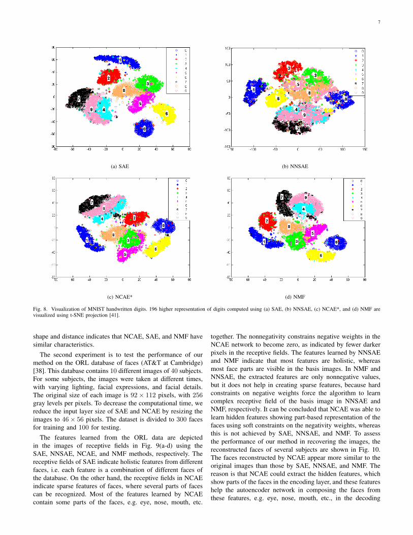
To better evaluate the hidden activities, Fig. 7 depicts thesparsity measured by the KL divergence of Eq. (6) for differentnumbers of hidden neurons in NCAE and SAE networks. Theresults indicate that the hidden activations in NCAE are moresparse than SAE, since JKL (p||p) is reduced significantly. Thismeans that the hidden neurons in NCAE are less activated thanin SAE when averaged over the full training set. In order toevaluate the ability of the proposed method in discovering thehidden structure of data in the original high-dimensional space,the distributions of MNIST digits in the higher representationlevel, i.e. hidden activities in SAE, NNSAE and NCAE neuralnetworks, and feature encoding of NMF (H), are visualizedin Fig. 8(a), 8(b), 8(c), and 8(d) for SAE, NNSAE, NCAE,and NMF, respectively. The figures show the reduced 196-dimensional higher representations of digits in 2D space usingt-distributed Stochastic Neighbor Embedding (t-SNE) projec-tion [41]. The comparison between these methods reveals thatthe distributions of digits for SAE, NCAE, and NMF are moresimilar to each other than NNSAE. It is clear that manifoldof digits in NNSAE have more overlap and more twists thanthe other methods. On the other hand, the manifolds of digits7, 9, 4 in NCAE are more linear than in SAE and NMF. Thecomparison between manifolds of other digits in terms of
7
(a) SAE (b) NNSAE
(c) NCAE* (d) NMF
Fig. 8. Visualization of MNIST handwritten digits. 196 higher representation of digits computed using (a) SAE, (b) NNSAE, (c) NCAE*, and (d) NMF arevisualized using t-SNE projection [41].
shape and distance indicates that NCAE, SAE, and NMF havesimilar characteristics.
The second experiment is to test the performance of ourmethod on the ORL database of faces (AT&T at Cambridge)[38]. This database contains 10 different images of 40 subjects.For some subjects, the images were taken at different times,with varying lighting, facial expressions, and facial details.The original size of each image is 92⇥ 112 pixels, with 256
gray levels per pixels. To decrease the computational time, wereduce the input layer size of SAE and NCAE by resizing theimages to 46⇥ 56 pixels. The dataset is divided to 300 facesfor training and 100 for testing.
The features learned from the ORL data are depictedin the images of receptive fields in Fig. 9(a-d) using theSAE, NNSAE, NCAE, and NMF methods, respectively. Thereceptive fields of SAE indicate holistic features from differentfaces, i.e. each feature is a combination of different faces ofthe database. On the other hand, the receptive fields in NCAEindicate sparse features of faces, where several parts of facescan be recognized. Most of the features learned by NCAEcontain some parts of the faces, e.g. eye, nose, mouth, etc.
together. The nonnegativity constrains negative weights in theNCAE network to become zero, as indicated by fewer darkerpixels in the receptive fields. The features learned by NNSAEand NMF indicate that most features are holistic, whereasmost face parts are visible in the basis images. In NMF andNNSAE, the extracted features are only nonnegative values,but it does not help in creating sparse features, because hardconstraints on negative weights force the algorithm to learncomplex receptive field of the basis image in NNSAE andNMF, respectively. It can be concluded that NCAE was able tolearn hidden features showing part-based representation of thefaces using soft constraints on the negativity weights, whereasthis is not achieved by SAE, NNSAE, and NMF. To assessthe performance of our method in recovering the images, thereconstructed faces of several subjects are shown in Fig. 10.The faces reconstructed by NCAE appear more similar to theoriginal images than those by SAE, NNSAE, and NMF. Thereason is that NCAE could extract the hidden features, whichshow parts of the faces in the encoding layer, and these featureshelp the autoencoder network in composing the faces fromthese features, e.g. eye, nose, mouth, etc., in the decoding

8
(a) SAE
(b) NNSAE
(c) NCAE*
(d) NMF
Fig. 9. 100 Receptive fields learned from the ORL Faces data set using (a) SAE, (b) NNSAE, (c) NCAE*, and (d) NMF. Black pixels indicate negativeweights, and white pixels indicate positive weights.
Fig. 10. Reconstruction of the ORL Faces test data using 300 receptive fields, using SAE (error=8.6447), NNSAE (error=15.7433), NCAE* (error=5.4944),and NMF (error=7.5653).
(a) ↵ = 0.003
(b) ↵ = 0.03
(c) ↵ = 0.3
Fig. 11. 100 Receptive fields learned from ORL Faces data set using NCAE for varying nonnegativity penalty coefficients (↵). Brighter pixels indicate largerweights.
layer. However, it is hard to compose the original face fromthe holistic features created by SAE, NNSAE, and NMF.
To investigate the effect of the nonnegativity constraintpenalty coefficient (↵) in NCAE for learning part-based rep-resentation, we test different values of ↵ to train NCAE. Thehidden features are depicted in Fig. 11. For this experiment,we increase ↵ logarithmically for 3 values in the range[0.003, . . . , 0.3]. The results indicate that by increasing ↵, theresulting features are more sparse, and decompose faces intosmaller parts. It is clear that the receptive fields in Fig. 11(c)are more sparse, and only show few parts of the faces. Thistest demonstrates that NCAE is able to extract different typesof eyes, noses, mouths, etc. from the face database.
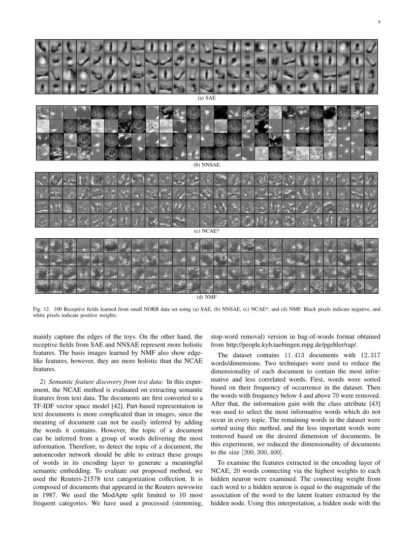
In the third experiment, we use the NORB normalized-
uniform dataset [39], which contains 24, 300 training examplesand 24, 300 test examples. This database contains images of50 toys from 5 generic categories: four-legged animals, humanfigures, airplanes, trucks, and cars. The training and testingsets are composed of 5 instances of each category. Each imageconsists of two channels, each of size 96⇥96 pixels. We takethe inner 64 ⇥ 64 pixels of each channel and resize it usingbicubic interpolation to 32⇥32 pixels that form a vector with2048 entries as the input. To evaluate the performance of themethod, we train an autoencoder using 100 hidden neuronsfor SAE, NNSAE, and NCAE, and also NMF with 100 basisvectors. The learned features are shown as receptive fields inFig. 12. The results indicate that the receptive fields learnedby NCAE are more sparse than SAE and NNSAE, since they
9
(a) SAE
(b) NNSAE
(c) NCAE*
(d) NMF
Fig. 12. 100 Receptive fields learned from small NORB data set using (a) SAE, (b) NNSAE, (c) NCAE*, and (d) NMF. Black pixels indicate negative, andwhite pixels indicate positive weights.
mainly capture the edges of the toys. On the other hand, thereceptive fields from SAE and NNSAE represent more holisticfeatures. The basis images learned by NMF also show edge-like features, however, they are more holistic than the NCAEfeatures.
2) Semantic feature discovery from text data: In this exper-iment, the NCAE method is evaluated on extracting semanticfeatures from text data. The documents are first converted to aTF-IDF vector space model [42]. Part-based representation intext documents is more complicated than in images, since themeaning of document can not be easily inferred by addingthe words it contains. However, the topic of a documentcan be inferred from a group of words delivering the mostinformation. Therefore, to detect the topic of a document, theautoencoder network should be able to extract these groupsof words in its encoding layer to generate a meaningfulsemantic embedding. To evaluate our proposed method, weused the Reuters-21578 text categorization collection. It iscomposed of documents that appeared in the Reuters newswirein 1987. We used the ModApte split limited to 10 mostfrequent categories. We have used a processed (stemming,
stop-word removal) version in bag-of-words format obtainedfrom http://people.kyb.tuebingen.mpg.de/pgehler/rap/.
The dataset contains 11, 413 documents with 12, 317
words/dimensions. Two techniques were used to reduce thedimensionality of each document to contain the most infor-mative and less correlated words. First, words were sortedbased on their frequency of occurrence in the dataset. Thenthe words with frequency below 4 and above 70 were removed.After that, the information gain with the class attribute [43]was used to select the most informative words which do notoccur in every topic. The remaining words in the dataset weresorted using this method, and the less important words wereremoved based on the desired dimension of documents. Inthis experiment, we reduced the dimensionality of documentsto the size [200, 300, 400].
To examine the features extracted in the encoding layer ofNCAE, 20 words connecting via the highest weights to eachhidden neuron were examined. The connecting weight fromeach word to a hidden neuron is equal to the magnitude of theassociation of the word to the latent feature extracted by thehidden node. Using this interpretation, a hidden node with the
10
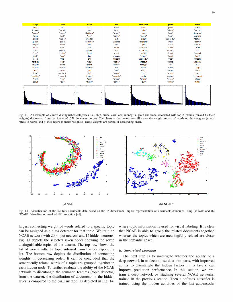
Fig. 13. An example of 7 most distinguished categories, i.e., ship, crude, earn, acq, money-fx, grain and trade associated with top 20 words (ranked by theirweights) discovered from the Reuters-21578 document corpus. The charts at the bottom row illustrate the weight impact of words on the category (x axisrefers to words and y axes refers to theirs weights). These weights are sorted in descending order.
(a) SAE (b) NCAE*
Fig. 14. Visualization of the Reuters documents data based on the 15-dimensional higher representation of documents computed using (a) SAE and (b)NCAE*. Visualization used t-SNE projection [41].
largest connecting weight of words related to a specific topiccan be assigned as a class detector for that topic. We train anNCAE network with 200 input neurons and 15 hidden neurons.Fig. 13 depicts the selected seven nodes showing the sevendistinguishable topics of the dataset. The top row shows thelist of words with the topic inferred from the correspondinglist. The bottom row depicts the distribution of connectingweights in decreasing order. It can be concluded that thesemantically related words of a topic are grouped together ineach hidden node. To further evaluate the ability of the NCAEnetwork to disentangle the semantic features (topic detector)from the dataset, the distribution of documents in the hiddenlayer is compared to the SAE method, as depicted in Fig. 14,
where topic information is used for visual labeling. It is clearthat NCAE is able to group the related documents together,whereas the topics which are meaningfully related are closerin the semantic space.
B. Supervised Learning
The next step is to investigate whether the ability of adeep network in to decompose data into parts, with improvedability to disentangle the hidden factors in its layers, canimprove prediction performance. In this section, we pre-train a deep network by stacking several NCAE networks,trained in the previous section. Then a softmax classifier istrained using the hidden activities of the last autoencoder
11
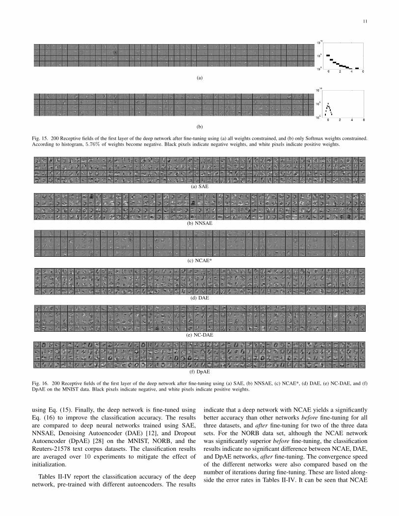
(a)
(b)
Fig. 15. 200 Receptive fields of the first layer of the deep network after fine-tuning using (a) all weights constrained, and (b) only Softmax weights constrained.According to histogram, 5.76% of weights become negative. Black pixels indicate negative weights, and white pixels indicate positive weights.
(a) SAE
(b) NNSAE
(c) NCAE*
(d) DAE
(e) NC-DAE
(f) DpAE
Fig. 16. 200 Receptive fields of the first layer of the deep network after fine-tuning using (a) SAE, (b) NNSAE, (c) NCAE*, (d) DAE, (e) NC-DAE, and (f)DpAE on the MNIST data. Black pixels indicate negative, and white pixels indicate positive weights.
using Eq. (15). Finally, the deep network is fine-tuned usingEq. (16) to improve the classification accuracy. The resultsare compared to deep neural networks trained using SAE,NNSAE, Denoising Autoencoder (DAE) [12], and DropoutAutoencoder (DpAE) [28] on the MNIST, NORB, and theReuters-21578 text corpus datasets. The classification resultsare averaged over 10 experiments to mitigate the effect ofinitialization.
Tables II-IV report the classification accuracy of the deepnetwork, pre-trained with different autoencoders. The results
indicate that a deep network with NCAE yields a significantlybetter accuracy than other networks before fine-tuning for allthree datasets, and after fine-tuning for two of the three datasets. For the NORB data set, although the NCAE networkwas significantly superior before fine-tuning, the classificationresults indicate no significant difference between NCAE, DAE,and DpAE networks, after fine-tuning. The convergence speedof the different networks were also compared based on thenumber of iterations during fine-tuning. These are listed along-side the error rates in Tables II-IV. It can be seen that NCAE
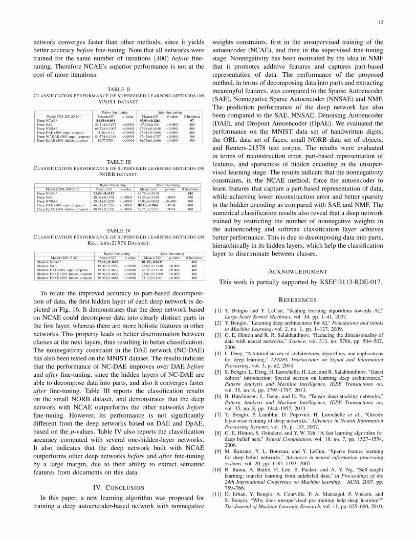
12
network converges faster than other methods, since it yieldsbetter accuracy before fine-tuning. Note that all networks weretrained for the same number of iterations (400) before fine-tuning. Therefore NCAE’s superior performance is not at thecost of more iterations.
TABLE IICLASSIFICATION PERFORMANCE OF SUPERVISED LEARNING METHODS ON
MNIST DATASET.
Before fine-tuning After fine-tuningModel (784-200-20-10) Mean±SD p-value Mean±SD p-value # Iterations
Deep NCAE* 84.83±0.094 97.91±0.1264 97Deep SAE 52.81±0.1277 <0.0001 97.29±0.091 <0.0001 400Deep NNSAE 69.72±0.1007 <0.0001 97.18±0.0648 <0.0001 400Deep DAE (50% input dropout) 11.26±0.14 <0.0001 97.11±0.0808 <0.0001 400Deep NC-DAE (50% input dropout) 84.37±0.1318 <0.0001 97.42±0.0757 <0.0001 106Deep DpAE (50% hidden dropout) 16.77.0784 <0.0001 96.73±0.1066 <0.0001 400
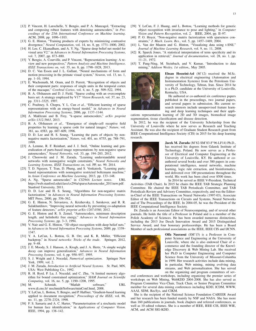
TABLE IIICLASSIFICATION PERFORMANCE OF SUPERVISED LEARNING METHODS ON
NORB DATASET.
Before fine-tuning After fine-tuningModel (2048-200-20-5) Mean±SD p-value Mean±SD p-value # Iterations
Deep NCAE* 75.54±0.1152 87.76±0.3613 242Deep SAE 20.00±0.1768 <0.0001 87.26±0.3109 0.0039 400Deep NNSAE 19.93±0.2230 <0.0001 79.00±0.0962 <0.0001 400Deep DAE (50% input dropout) 44.03±0.1553 <0.0001 88.11±0.3861 0.0508 400Deep DpAE (50% hidden dropout) 49.49±0.1437 <0.0001 87.75±0.2767 0.9454 400
TABLE IVCLASSIFICATION PERFORMANCE OF SUPERVISED LEARNING METHODS ON
REUTERS-21578 DATASET.
Before fine-tuning After fine-tuningModel (200-15-10) Mean±SD p-value Mean±SD p-value # Iterations
Shallow NCAE* 57.18±0.3639 81.15±0.1637 400Shallow SAE 39.00±0.2255 <0.0001 78.60±0.2143 <0.0001 400Shallow DAE (50% input dropout) 39.00±0.3617 <0.0001 76.35±0.1918 <0.0001 400Shallow DpAE (20% hidden dropout) 39.00±0.4639 <0.0001 78.04±0.1709 <0.0001 400Shallow DpAE (50% hidden dropout) 39.00±0.3681 <0.0001 72.12±0.2901 <0.0001 400.
To relate the improved accuracy to part-based decomposi-tion of data, the first hidden layer of each deep network is de-picted in Fig. 16. It demonstrates that the deep network basedon NCAE could decompose data into clearly distinct parts inthe first layer, whereas there are more holistic features in othernetworks. This property leads to better discrimination betweenclasses at the next layers, thus resulting in better classification.The nonnegativity constraint in the DAE network (NC-DAE)has also been tested on the MNIST dataset. The results indicatethat the performance of NC-DAE improves over DAE before
and after fine-tuning, since the hidden layers of NC-DAE areable to decompose data into parts, and also it converges fasterafter fine-tuning. Table III reports the classification resultson the small NORB dataset, and demonstrates that the deepnetwork with NCAE outperforms the other networks before
fine-tuning. However, its performance is not significantlydifferent from the deep networks based on DAE and DpAE,based on the p-values. Table IV also reports the classificationaccuracy computed with several one-hidden-layer networks.It also indicates that the deep network built with NCAEoutperforms other deep networks before and after fine-tuningby a large margin, due to their ability to extract semanticfeatures from documents on this data.
IV. CONCLUSION
In this paper, a new learning algorithm was proposed fortraining a deep autoencoder-based network with nonnegative
weights constraints, first in the unsupervised training of theautoencoder (NCAE), and then in the supervised fine-tuningstage. Nonnegativity has been motivated by the idea in NMFthat it promotes additive features and captures part-basedrepresentation of data. The performance of the proposedmethod, in terms of decomposing data into parts and extractingmeaningful features, was compared to the Sparse Autoencoder(SAE), Nonnegative Sparse Autoencoder (NNSAE) and NMF.The prediction performance of the deep network has alsobeen compared to the SAE, NNSAE, Denoising Autoencoder(DAE), and Dropout Autoencoder (DpAE). We evaluated theperformance on the MNIST data set of handwritten digits,the ORL data set of faces, small NORB data set of objects,and Reuters-21578 text corpus. The results were evaluatedin terms of reconstruction error, part-based representation offeatures, and sparseness of hidden encoding in the unsuper-vised learning stage. The results indicate that the nonnegativityconstraints, in the NCAE method, force the autoencoder tolearn features that capture a part-based representation of data,while achieving lower reconstruction error and better sparsityin the hidden encoding as compared with SAE and NMF. Thenumerical classification results also reveal that a deep networktrained by restricting the number of nonnegative weights inthe autoencoding and softmax classification layer achievesbetter performance. This is due to decomposing data into parts,hierarchically in its hidden layers, which help the classificationlayer to discriminate between classes.
ACKNOWLEDGMENT
This work is partially supported by KSEF-3113-RDE-017.
REFERENCES
[1] Y. Bengio and Y. LeCun, “Scaling learning algorithms towards AI,”Large-Scale Kernel Machines, vol. 34, pp. 1–41, 2007.
[2] Y. Bengio, “Learning deep architectures for AI,” Foundations and trends
in Machine Learning, vol. 2, no. 1, pp. 1–127, 2009.[3] G. E. Hinton and R. R. Salakhutdinov, “Reducing the dimensionality of
data with neural networks,” Science, vol. 313, no. 5786, pp. 504–507,2006.
[4] L. Deng, “A tutorial survey of architectures, algorithms, and applicationsfor deep learning,” APSIPA Transactions on Signal and Information
Processing, vol. 3, p. e2, 2014.[5] S. Bengio, L. Deng, H. Larochelle, H. Lee, and R. Salakhutdinov, “Guest
editors’ introduction: Special section on learning deep architectures,”Pattern Analysis and Machine Intelligence, IEEE Transactions on,vol. 35, no. 8, pp. 1795–1797, 2013.
[6] B. Hutchinson, L. Deng, and D. Yu, “Tensor deep stacking networks,”Pattern Analysis and Machine Intelligence, IEEE Transactions on,vol. 35, no. 8, pp. 1944–1957, 2013.
[7] Y. Bengio, P. Lamblin, D. Popovici, H. Larochelle et al., “Greedylayer-wise training of deep networks,” Advances in Neural Information
Processing Systems, vol. 19, p. 153, 2007.[8] G. E. Hinton, S. Osindero, and Y. W. Teh, “A fast learning algorithm for
deep belief nets,” Neural Computation, vol. 18, no. 7, pp. 1527–1554,2006.
[9] M. Ranzato, Y. L. Boureau, and Y. LeCun, “Sparse feature learningfor deep belief networks,” Advances in neural information processing
systems, vol. 20, pp. 1185–1192, 2007.[10] R. Raina, A. Battle, H. Lee, B. Packer, and A. Y. Ng, “Self-taught
learning: transfer learning from unlabeled data,” in Proceedings of the
24th International Conference on Machine learning. ACM, 2007, pp.759–766.
[11] D. Erhan, Y. Bengio, A. Courville, P. A. Manzagol, P. Vincent, andS. Bengio, “Why does unsupervised pre-training help deep learning?”The Journal of Machine Learning Research, vol. 11, pp. 625–660, 2010.
13
[12] P. Vincent, H. Larochelle, Y. Bengio, and P. A. Manzagol, “Extractingand composing robust features with denoising autoencoders,” in Pro-
ceedings of the 25th International Conference on Machine learning.ACM, 2008, pp. 1096–1103.
[13] G. E. Hinton, “Training products of experts by minimizing contrastivedivergence,” Neural Computation, vol. 14, no. 8, pp. 1771–1800, 2002.
[14] H. Lee, C. Ekanadham, and A. Y. Ng, “Sparse deep belief net model forvisual area V2.” in Advances in Neural Information Processing Systems,vol. 7, 2007, pp. 873–880.
[15] Y. Bengio, A. Courville, and P. Vincent, “Representation learning: A re-view and new perspectives,” Pattern Analysis and Machine Intelligence,
IEEE Transactions on, vol. 35, no. 8, pp. 1798–1828, 2013.[16] D. C. Van Essen and J. L. Gallant, “Neural mechanisms of form and
motion processing in the primate visual system,” Neuron, vol. 13, no. 1,pp. 1–10, 1994.
[17] E. Wachsmuth, M. Oram, and D. Perrett, “Recognition of objects andtheir component parts: responses of single units in the temporal cortexof the macaque,” Cerebral Cortex, vol. 4, no. 5, pp. 509–522, 1994.
[18] B. A. Olshausen and D. J. Field, “Sparse coding with an overcompletebasis set: A strategy employed by V1?” Vision Research, vol. 37, no. 23,pp. 3311–3325, 1997.
[19] C. Poultney, S. Chopra, Y. L. Cun et al., “Efficient learning of sparserepresentations with an energy-based model,” in Advances in Neural
Information Processing Systems, 2006, pp. 1137–1144.[20] A. Makhzani and B. Frey, “k-sparse autoencoders,” arXiv preprint
arXiv:1312.5663, 2013.[21] B. A. Olshausen et al., “Emergence of simple-cell receptive field
properties by learning a sparse code for natural images,” Nature, vol.381, no. 6583, pp. 607–609, 1996.
[22] D. D. Lee and H. S. Seung, “Learning the parts of objects by non-negative matrix factorization,” Nature, vol. 401, no. 6755, pp. 788–791,1999.
[23] A. Lemme, R. F. Reinhart, and J. J. Steil, “Online learning and gen-eralization of parts-based image representations by non-negative sparseautoencoders,” Neural Networks, vol. 33, pp. 194–203, 2012.
[24] J. Chorowski and J. M. Zurada, “Learning understandable neuralnetworks with nonnegative weight constraints,” Neural Networks and
Learning Systems, IEEE Transactions on, vol. PP, no. 99, 2014.[25] T. D. Nguyen, T. Tran, D. Phung, and S. Venkatesh, “Learning parts-
based representations with nonnegative restricted boltzmann machine,”in Asian Conference on Machine Learning, 2013, pp. 133–148.
[26] A. Ng, “Sparse autoencoder,” in CS294A Lecture notes. URLhttps://web.stanford.edu/class/cs294a/sparseAutoencoder 2011new.pdf:Stanford University, 2011.
[27] D. D. Lee and H. S. Seung, “Algorithms for non-negative matrixfactorization,” in Advances in Neural Information Processing Systems.MIT Press, 2000, pp. 556–562.
[28] G. E. Hinton, N. Srivastava, A. Krizhevsky, I. Sutskever, and R. R.Salakhutdinov, “Improving neural networks by preventing co-adaptationof feature detectors,” arXiv preprint arXiv:1207.0580, 2012.
[29] G. E. Hinton and R. S. Zemel, “Autoencoders, minimum descriptionlength, and helmholtz free energy,” Advances in Neural Information
Processing Systems, pp. 3–3, 1994.[30] V. Nair and G. E. Hinton, “3D object recognition with deep belief nets.”
in Advances in Neural Information Processing Systems, 2009, pp. 1339–1347.
[31] Y. A. LeCun, L. Bottou, G. B. Orr, and K. R. Muller, “Efficientbackprop,” in Neural networks: Tricks of the trade. Springer, 2012,pp. 9–48.
[32] J. E. Moody, S. J. Hanson, A. Krogh, and J. A. Hertz, “A simple weightdecay can improve generalization,” Advances in Neural Information
Processing Systems, vol. 4, pp. 950–957, 1995.[33] S. J. Wright and J. Nocedal, Numerical optimization. Springer New
York, 1999, vol. 2.[34] J. M. Zurada, Introduction to Artificial Neural Systems. St. Paul, MN,
USA: West Publishing Co., 1992.[35] R. H. Byrd, P. Lu, J. Nocedal, and C. Zhu, “A limited memory algo-
rithm for bound constrained optimization,” SIAM Journal on Scientific
Computing, vol. 16, no. 5, pp. 1190–1208, 1995.[36] M. Schmidt, “Matlab software,” URL
www.di.ens.fr/ mschmidt/Software/minConf.html, 2008.[37] Y. LeCun, L. Bottou, Y. Bengio, and P. Haffner, “Gradient-based learning
applied to document recognition,” Proceedings of the IEEE, vol. 86,no. 11, pp. 2278–2324, 1998.
[38] F. S. Samaria and A. C. Harter, “Parameterisation of a stochastic modelfor human face identification,” in Applications of Computer Vision.IEEE, 1994, pp. 138–142.
[39] Y. LeCun, F. J. Huang, and L. Bottou, “Learning methods for genericobject recognition with invariance to pose and lighting,” in Computer
Vision and Pattern Recognition, vol. 2. IEEE, 2004, pp. II–97.[40] P. O. Hoyer, “Non-negative matrix factorization with sparseness con-
straints,” J. Mach. Learn. Res., vol. 5, pp. 1457–1469, 2004.[41] L. Van der Maaten and G. Hinton, “Visualizing data using t-SNE.”
Journal of Machine Learning Research, vol. 9, no. 11, 2008.[42] K. Sparck Jones, “A statistical interpretation of term specificity and its
application in retrieval,” Journal of documentation, vol. 28, no. 1, pp.11–21, 1972.
[43] T. Pang-Ning, M. Steinbach, and V. Kumar, “Introduction to datamining,” Addison Wesley, 1st edition,, May 2005.
Ehsan Hosseini-Asl (M’12) received the M.Sc.degree in electrical engineering (Automation andInstrumentation Systems) from the Petroleum Uni-versity of Technology, Tehran, Iran. Since 2014 heis a Ph.D. candidate at the University of Louisville,Kentucky, USA.
He authored or co-authored six conference paperspublished in the proceedings, two journal papers,and several papers in submission. His current re-search interests include unsupervised feature learn-ing and deep learning techniques and their appli-
cations representation learning of 2D and 3D images, biomedical imagesegmentation, tissue classification and disease detection.
In 2012, he was the recipient of the University Scholarship from theUniversity of Louisville where he now serves as Research and TeachingAssistant. He was also the recipient of Graduate Student Research grant fromIEEE Computational Intelligence Society (CIS) in 2015 for his deep learningresearch.
Jacek M. Zurada (M’82-SM’83-F’96-LF14) Ph.D.,has received his degrees from Gdansk Institute ofTechnology, Poland. He now serves as a Profes-sor of Electrical and Computer Engineering at theUniversity of Louisville, KY. He authored or co-authored several books and over 380 papers in com-putational intelligence, neural networks, machinelearning, logic rule extraction, and bioinformatics,and delivered over 100 presentations throughout theworld. His work has been cited over 8500 times.
In 2014 he served as IEEE V-President, TechnicalActivities (TAB Chair). In 2015 he chairs the IEEE TAB Strategic PlanningCommittee. He chaired the IEEE TAB Periodicals Committee, and TABPeriodicals Review and Advisory Committee, respectively, and was the Editor-in-Chief of the IEEE Transactions on Neural Networks (1997-03), AssociateEditor of the IEEE Transactions on Circuits and Systems, Neural Networksand of The Proceedings of the IEEE. In 2004-05, he was the President of theIEEE Computational Intelligence Society.
Dr. Zurada is an Associate Editor of Neurocomputing, and of several otherjournals. He holds the title of a Professor in Poland and is a member of thePolish Academy of Sciences. He has been awarded numerous distinctions,including the 2013 Joe Desch Innovation Award and 2015 DistinguishedService Award, and four honorary professorships. He has been a BoardMember of such professional associations as the IEEE, IEEE CIS and IJCNN.
Olfa Nasraoui (SM’15) is a Professor in Com-puter Science and Engineering at the University ofLouisville, where she is also endowed Chair of e-commerce and the founding director of the Knowl-edge Discovery & Web Mining Lab. She receivedher Ph.D in Computer Engineering and ComputerScience from the University of Missouri-Columbiain 1999. Her research activities include data mining,in particular, Web mining, mining evolving datastreams, and Web personalization. She has servedon the organizing and program committees of sev-
eral conferences and workshops, including organizing the premier series ofworkshops on Web Mining, WebKDD 2004-2008. She has also served asProgram Committee Vice-Chair, Track Chair, or Senior Program Committeemember for several data mining conferences including KDD, ICDM, WWW,AAAI, SDM, RecSys, and CIKM.
She is the recipient of the National Science Foundation CAREER Awardand her research has been funded mainly by NSF and NASA. She has morethan 160 publications in journals, book chapters and refereed conferences, aswell as 10 edited volumes. She is a member of IEEE, IEEE CIS, IEEE WIE,ACM, and ACM SIG-KDD.