DEEP NEURAL NETWORKS FOR ABOVE-GROUND DETECTION IN …

DEEP NEURAL NETWORKS FOR ABOVE-GROUND DETECTION IN VERY HIGH

SPATIAL RESOLUTION DIGITAL ELEVATION MODELS

D. Marmanis a,b, F. Adam a, M. Datcu a, T. Esch a, U. Stilla b

a EOC, German Aerospace Center, Wessling, Germany - (Dimitrios. Marmanis, Fathalrahman.Adam,

Mihai.Datcu, Thomas.Esch)@dlr.de b Chair of Photogrammetry & Remote Sensing, Technische Universitaet Muenchen, Germany - [email protected]

Commission III, WG III/7

KEY WORDS: Deep Learning, Multilayer Perceptrons, Ground Filtering, DEM, Classification

ABSTRACT:

Deep Learning techniques have lately received increased attention for achieving state-of-the-art results in many classification

problems, including various vision tasks. In this work, we implement a Deep Learning technique for classifying above-ground

objects within urban environments by using a Multilayer Perceptron model and VHSR DEM data. In this context, we propose a novel

method called M-ramp which significantly improves the classifier’s estimations by neglecting artefacts, minimizing convergence

time and improving overall accuracy. We support the importance of using the M-ramp model in DEM classification by conducting a

set of experiments with both quantitative and qualitative results. Precisely, we initially train our algorithm with random DEM tiles

and their respective point-labels, considering less than 0.1% over the test area, depicting the city center of Munich (25 km2).

Furthermore with no additional training, we classify two much larger unseen extents of the greater Munich area (424 km2) and

Dongying city, China (257 km2) and evaluate their respective results for proving knowledge-transferability. Through the use of M-

ramp, we were able to accelerate the convergence by a magnitude of 8 and achieve a decrease in above-ground relative error by

24.8% and 5.5% over the different datasets.

1. INTRODUCTION

1.1 Previous Work

Building and ground detection is a crucial step for many

applications in the analysis of Digital Elevation Models (DEM)

such as urban monitoring, real estate, disaster response and 3D

city reconstruction. Automatic methods that can robustly detect

above-ground objects in such context could prove very valuable

as extended human labour and the large cost involved could be

omitted. In the literature there is a plethora of such proposed

methods where different techniques and input data are

considered. Belli et al. (2001) proposed a method to extract and

model above ground objects by estimating the Digital Terrain

Model (DTM) from a DEM obtained from stereoscopic aerial

colour images. The ground surface is estimated through the use

of 2D harmonics and Fourier series. With respect to this

framework, above-ground objects are considered outliers.

Zingaretti et al. (2007) proposed a method using raw LIDAR

data where a boosted decision tree-classifier was used to

identify optimal classification rules and separate data in

buildings, ground, and vegetation classes when applied over

segmented data. Hao et al. (2009) was able to accurately detect

the buildings using a combination of filtering, clustering, and

thresholding over a LIDAR dataset. Baillard and Maitre (1999)

used a stereopair of images to initially compute the DEM model

and then segmented the above-ground objects using a Markov

Random Field model. Afterwards, they differentiated between

vegetation and buildings through the use of radiometric

analysis. Ortner et al. (2007) proposed a method for directly

extracting vectorial land registers from DEM data using an

energy minimization model, where the assumption that

buildings are composed by simple rectangles is considered.

Furthermore, this method was improved by Tournaire et al.

(2010), so it can process data more efficiently.

Despite the extended work in the field, above-ground and

building detection still remains an open research area. In our

view, algorithms that make strong assumptions upon the size or

shape of the high-structures in the data are unlikely to robustly

detect above-ground structures in different urban scenes.

Therefore, our goal in this work is to construct a generic

framework, without making presumptions upon the size, shape,

extent or resolution of the input DEM data.

1.2 Deep Neural Networks for Above-Ground Detection

In this work, we investigate the potential of Deep Neural

Network (DNN) systems in above-ground object detection

within urban environments. Specifically, our target is to

separate the high-standing structures (trees and building) from

their surrounding terrain over large data extents with high-

accuracy. To achieve this goal we construct a generic algorithm

based on Deep Neural Networks and argue that such a model is

capable for detecting above-ground objects over unseen areas,

even when data are generated using different sensors. To

support our claim we conduct a series of experiments using two

very heterogeneous DEMs acquired by different sensors with

different resolutions.

The rest of this work is organized as follows. Chapter 2

analyses the DNN algorithm in detail. Chapter 3 discusses the

algorithms and workflow processes used for above-ground

object detection. Chapter 4 and 5 deal with the description of

test datasets and their experimental results. We end this work in

Chapter 6 where we discuss our results and summarize our

contributions.

ISPRS Annals of the Photogrammetry, Remote Sensing and Spatial Information Sciences, Volume II-3/W4, 2015 PIA15+HRIGI15 – Joint ISPRS conference 2015, 25–27 March 2015, Munich, Germany

This contribution has been peer-reviewed. The double-blind peer-review was conducted on the basis of the full paper. doi:10.5194/isprsannals-II-3-W4-103-2015

103

mailto:[email protected]

2. THE DEEP LEARNING ALGORITHM

2.1 Deep Neural Networks

Deep Neural Networks is a sub-field of Deep Learning (DL)

expressed by ordinary Artificial Neural Networks with multiple

hidden-layers. These multiprocessing stage distributed

architectures allow the system to learn hierarchical

representations by combining features of different abstraction

levels generated by the various layers. The key element of such

Deep Learning systems is the projection of their input data into

a new space through the use of a non-linear function on each

processing stage (hidden-layer). Via such a procedure, DNNs

are capable of effectively extracting features over high-

dimensional structured data and achieve high performance in

various classification tasks.

2.2 Multilayer Perceptrons for Above-Ground Object

Detection

Probably the most broadly known architecture in the context of

Artificial Neural Networks is the Multilayer Perceptron

algorithm (MLP) which is a discriminative, supervised

classification and regression model trained through standard

Backpropagation (Rumelhart et al., 1986). Furthermore, MLPs

are fully connected networks which mean that they relate each

and every variable of a hidden-layer to all variables in the

proceeding layer. Interestingly, MLPs are a modification of the

standard Linear Perceptrons, introduced by Rosenblatt in the

1950s (Rosenblatt, 1957)

Despite their overall simplicity when compared to more

complex and statistically promising Deep Leaning architectures,

(e.g. Deep Belief Networks, Convolutional Neural Networks,

etc.) with respect to our experiments, MLPs formulate a very

concrete framework for accurately classifying large amounts of

remotely sensed data, such as above-ground objects.

Furthermore, their computational simplicity allowed us to

conduct a very large number of different experiments that

significantly improved our results and strengthened our

understanding over these methods. Considering all these

aspects, we concluded that it should suffice to focus on MLPs

for conducting all our experiments, keeping in mind that other

DL architectures may result in quantitatively better outcomes.

2.3 Deep Multilayer Perceptron

As long as Artificial Neural Networks are implemented using a

single hidden layer, as commonly found in most of the software

packages (e.g. MATLAB Neural Networks toolbox), the user

has limited choices concerning the network’s architecture,

mainly selecting the number of hidden nodes or different

optimization algorithms. However when one decides upon a

deep architecture, finding an ideal local minimum in the error

surface becomes a much harder task for the algorithm due to

multiple non-linearities. Therefore in DL, it’s essential for one

to understand the individual components forming the neural

network and then decide upon different techniques for achieving

a good classification performance. Below, we refer to these

individual parts which form our MLP model.

2.4 Layer Architecture

Our MLP is composed by 8 layers where layer-1 is the input,

layer-8 is the output (Softmax Classifier) and the rest are hidden

non-linear layers. The intuition lying behind this architecture is

that the MLP model will be able to construct high level features,

allowing it to adequately generalize over unseen data, even

when trained with very few training data.

Formally, a MLP is a function h, that maps an input vector x,

to a label vector y, through a set of non-linear functions f, with

parameters W and b (weights and bias terms). Concretely, a

single-layer neural network is expressed mathematically as:

ℎ𝑊,𝑏(𝑥) = 𝑓 (∑ 𝑊𝑖𝑥𝑖 + 𝑏

𝑖

) (1)

2.4.1 ReLU Activation Function: One option for the non-

linear activation function in a deep MLP network is the

Rectified-Linear Unit function (ReLU) which has some strong

advantages towards the most frequently used sigmoid and

hyperbolic-tangent activations. Specifically ReLU is preferable

due to its sparse activation properties, it does not saturate or

suffer from the vanishing gradient problem and it’s

computationally more efficient with respect to construction of

large networks. The rectified linear function is denoted by:

𝑓(𝑥) = max(𝑥, 0) (2)

2.5 Learning the Weights – Model Optimization

Our classification algorithm is trained by adjusting its weights

using the Backpropagation algorithm (Rumelhart et al., 1986)

with mini-batch gradient descent and a standard quadratic cost

function for penalizing over misclassified examples.

2.6 Regularization

One weakness that all neural networks exhibit is their tendency

to strongly overfit the training data. Therefore, in order to

prevent this from occurring, multiple regularization techniques

have to be employed, as suggested by the literature. Due to our

limited training data, our model is very venerable to such

overfitting phenomena therefore regularization becomes a

crucial issue. Below we briefly present all regularization

methods used in this study.

2.6.1 Weight Decay: Weight Decay (namely L2 regularization)

is a common choice for including an additional term to the loss

function by which large weights are penalized more, hence

avoided by the system. The effect is that eventually the weights

converge to smaller absolute values that would have done

otherwise. Below, the loss-function including a weight-decay

term is shown:

𝐸(𝑊, 𝑏) =1

2𝑚 ∑‖𝑦𝑖 − ℎ(𝑥𝑖 ; 𝑊, 𝑏)‖2 +

𝜆

2 ∑ 𝑊𝑙

2 (3)

𝐿−1

𝑙=1

𝑚

𝑖=1

Where m is the total number of training examples, L denotes the

respective layer in the network and 𝜆 is the weight decay

coefficient.

2.6.2 Momentum: A powerful method to avoid local minima

and speed-up convergence is to use yet another regularization

method, called momentum. Accordingly, by adding a

momentum term in the loss function, one can avoid fluctuations

between the weight-updates through the epochs during training.

This is implemented by partially considering the effect of the

previous weight update to the current gradient computation

(epoch). Mathematically this is expressed as:

∆𝑊(𝑡 + 1) = 𝑊 − 𝛼∂𝐸

𝜕𝑊+ 𝛽∆𝑊(𝑡) − 𝜆𝑊(𝑡) (4)



104

Where parameter t denotes the epochs, W the weight matrix, E

the loss-function and α, β 𝜆 are the learning rate, momentum

and weight-decays coefficients respectively.

2.6.3 Max-norm: Even though momentum can be a powerful

technique for speeding up convergence and helping avoid local

minima, this can cause the weight to grow very large (Srebro et

al., 2005). A good solution for this problem is given by Max-

norm regularization which constrains the sum of all weights

connected to a unit to be smaller than a pre-defined constant.

This can be mathematically expressed as:

𝑁(𝑊) = min ((∑ 𝑊𝑖,𝑗(𝐿)

), 𝜇

𝑗

) (5)

Where i denotes a particular unit in the network, j a certain

weight-connection and L the respective layer. The maximum

allowed norm-value is defined by the μ variable. Typically,

good values for constraining the max-norm are within the range

of 3 and 4.

2.6.4 Dropout: Using a large number of units on each hidden

layer is considered an advantage as the system learns very

“powerful” representations, however to avoid extensive

overfitting one should also employ a regularization technique

called ‘Dropout’. This method stochastically removes a

percentage of the initial network units and their respective

connecting-weights and can be seen as training an exponential

number of “thinned” networks which extensively share the same

weights (Srivastava et al., 2014). So for a neural network with n

units, dropout actually implements a collection of 2n thinned

neural networks with O(n2) or less number of units. Within this

framework, one can then train very large networks without the

concern of overfitting.

2.7 Network Hyperparameter Random Search

Finding a good set of hyperparameters for training an MLP

model is probably one of the toughest aspects when one

considers DL. Since there isn't any concrete rule for defining

them, one can implement either a brute-force method (grid-

search) or a random-search within a predefined range of values.

For standardizing our set of parameters, we used a random

search method and the best values found over a validation

dataset were used throughout our experiments. These values are

listed in the Table 1 below.

Hyperparameters Value

Dimension hidden h1 550 nodes





Dimension hidden h6 Size of input vector

Drop-out probability input 72 %

Drop-out probability h1 57 %





Weight Decay 0.001635

Initial Momentum 0.256

Final Momentum 0.5759

Start Epoch Momentum 5

Saturate Momentum Epoch 38

Learning Rate 0.244

Table 1. Standardized MLP hyperparameters

3. METHODOLOGY

3.1 Processing Steps

This section presents all the individual steps of our workflow

process. Specifically, methods for merging and enhancing

individual prediction are discussed in details, in addition to a

novel method presented for improving overall accuracy and

model convergence. The complete processing steps of our

method are summarized in the diagram of Figure 2.

3.2 Improving Classification with M-ramp

Inspired by the idea that DNNs construct better feature

representations when provided with an artificial destructed input

(Vincent et al., 2008), we expanded this concept by artificially

transforming the elevation of our input DEM model to partially

mimic this behaviour. More precisely, by introducing intense

artificial relief to the initial elevation model, we are forcing the

MLP to detect strong dependencies and patterns that

characterize above-ground objects within the urban environment

and omit noise artefacts and less expressive features robustly.

Such a hypothesis is logical considering the high dimensionality

and redundancy generally contained within image data.

We cluster these artificial relief alterations/regularization

methods under the name M-ramp (Make a ramp), as ramps are

probably the simplest modification one can introduce over an

elevation model. To our knowledge, there isn’t any previous

study considering this kind of artificial relief transformations for

delineating features from DEMs, despite the fact that in

machine learning literature there is extensive research for

constructing transformation invariant feature detectors (Dalal et

al., 2005). Even though M-ramp method can be seen as a noise-

corruptor applied over an input image, considering the distinct

nature of 3D-elevation models, one can strongly experiment

with large variations over the input that probably would not

make sense over a set of multispectral images. Furthermore, our

experiments suggest that a DEM classification could strongly

benefit from such artificial relief generation, especially when

extended modifications are applied over the input data. The gain

from using M-ramp alterations affects the above-ground

detection in four distinct ways.

i) Speeds-up model’s convergence by a large factor

ii) Helps the model avoid localized, non-regular errors

iii) Increases overall detection accuracy

iv) Generates “new” data

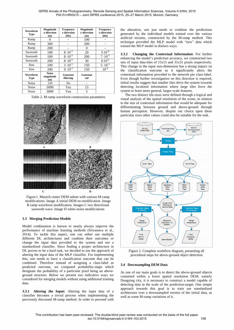
To better understand the impacts and benefits of M-ramp

models, we constructed a set of randomly modified DEMs

where different types of template-waveforms (with varying

magnitudes & frequencies) were considered along the

horizontal and vertical image dimensions. Continuously, these

artificially generated DEMs are appended over the initial DEM,

creating the final M-ramp models (Figure 1). At this point, it is

important to underline that our M-ramp models were randomly

designed without conducting any prior study regarding their

effects over the accuracy of the above-ground detection

problem. Therefore, their positive impact towards our

classification results wasn’t guaranteed. In addition, it is

important to note that the MLP hyperparameters were set using

initial untransformed data, hence the MLP is not optimally

tuned for these particular M-ramps.

All different construction parameters of the M-ramps DEM

models considered in this study are summarized in Table 2.



105

Waveform

Type

Magnitude

x-direction

(m)

Frequency

x direction

(Hz)

Magnitude

y-direction

(m)

Frequency

y-direction

(Hz)

Ramp 0 - 100 -

Ramp 300 - 200 -

Ramp 200 - 0 - Sawtooth 100 8 ∙10-5 20 5∙10-6 Sawtooth 100 8 ∙10-5 200 7 ∙10-5 Sawtooth 200 8 ∙10-5 30 6∙10-4

Sine 100 3 ∙10-5 150 5 ∙10-5 Sine 200 9 ∙10-5 150 10-4

Waveform

Type

Noise

magnitude

(m)

Gaussian

filtering

Gaussian

std

Noise 150 No -

Noise 5000 Yes 15

Noise 3000 Yes 5

Table 2. M-ramp waveform construction parameters

3.3 Merging Prediction Models

Model combination is known to nearly always improve the

performance of machine learning methods (Srivastava et al.,

2014). To tackle this aspect, one can either use multiple

different DL architectures and combine their outcomes or

change the input data provided to the system and use a

standardized classifier. Since finding a proper architecture in

DL proves to be a hard task, we decided to use the approach of

altering the input data of the MLP classifier. For implementing

this, one needs to have a classification outcome that can be

combined. Therefore instead of assigning a class-label as

predicted outcome, we computed probability-maps which

designate the probability of a particular pixel being an above-

ground structure. Below we present two indicative ways we

considered for merging models without using additional training

data.

3.3.1 Altering the Input: Altering the input data of a

classifier becomes a trivial process when implementing the

previously discussed M-ramp method. In order to proceed with

the alteration, one just needs to combine the predictions

generated by the individual models trained over the various

artificial terrains, constructed by the M-ramp method. This

technique provided the MLP model with “new” data which

trained the MLP model in distinct ways.

3.3.2 Changing the Contextual Information: For further

enhancing the model’s prediction accuracy, we constructed two

sets of input data-tiles of 15x15 and 31x31 pixels respectively.

This change in the input size-dimension has a strong impact on

the classification outcome as it significantly alters the

contextual information provided to the network per class-label.

Even though further investigation on this direction is required,

initial results suggest that smaller tiles drive the system towards

detecting localized information where large tiles force the

system to learn more general, larger-scale features.

The two distinct tile-sizes were defined through a logical and

visual analysis of the spatial resolution of the scene, in relation

to the size of contextual information that would be adequate for

differentiating between ground and above-ground through

human perception. However, despite our choice upon these

particular sizes other values could also be suitable for the task.

Figure 2. Complete workflow diagram, presenting all

procedural steps for above-ground object detection

3.4 Downsampling DEM Data

As one of our main goals is to detect the above-ground objects

contained within a lower spatial resolution DEM, namely

Dongying city, it is necessary to construct a model capable of

detecting data in the scale of the prediction-target. One simple

approach towards this goal is to train our standardized

architecture over a downsampled version of the initial data, as

well as some M-ramp variations of it.

A B

C D

Figure 1. Munich center DEM subset with various M-ramp

modifications. Image A initial DEM no-modification. Image

B ramp waveform modification. Images C two directional

sawtooth wave. Image D white-noise modifications



106

We found the downsampling step to be crucial for

predicting data with significantly different resolutions like the

ones considered in our experiments with a different scale-factor

equal to 16 (Munich 1x1 m2/pixel, Dongying 4x4 m2/pixel).

However, preliminary experiments suggest that when data with

small variations in resolution are considered, the algorithm can

predict scenes accurately throughout the different spatial-scales.

Nevertheless, the spatial invariance of the method is not

investigated further in this study

4. STUDY AREA

4.1 Study Area and Training Challenges

In our experiments, we used two very heterogeneous DEMs,

one delineating the urban and peri-urban area of Munich with an

extent of 424 km2 and spatial a resolution of 1-meter, as well as

a DEM of Dongying city in China, extending over an 257 km2

with a spatial resolution of 4-meters. Our hypothesis is that a

trained Deep Neural Network will be able to correctly detect all

above-ground structures in both Dongying and Munich datasets

under the following two-constrains:

i) Limit potential training area to a small subset of Munich

with an extent of 25 km2

ii) Only allow the classifier to sample 20000 random single

pixel-labels from this subset and use it for training

(comprise ~0.08% of Munich subset or ~0.005% of

complete Munich data)

The Munich subset we selected depicts the city center of

Munich (extent ~25 km2). Additionally, for detecting the above-

ground objects in Dongying dataset, we trained the very same

MLP model over a downsampled version of the Munich subset

(downsampled to 4-meters), using again 20000 randomly

selected point-samples.

4.2 Information on DEMs

The first dataset of this study is a VHSR DEM produced from

optical stereotypical, aerial images with a ground resolution of

1-meter. This data covers the greater area of Munich with an

overall extent of 424 km2 (22800 x 18600 pixels). Additionally,

in order to test our prediction model over a different urban

landscape, a second DEM of 4-meters resolution was also

considered. The latter was generated from a stereopair of

Pleiades-sensor optical images and depicts the complete extent

of Dongying city, located in Yellow River Delta, China. The

Dongying dataset covers an area of about 257 km2 and has very

different architectural characteristics compared to the Munich

dataset. Precisely, apart from the different resolution of the data

which significantly affects the level of details, the Munich

dataset is rather elevated with about 100 meter height difference

between its north and south side. Comparatively, the Dongying

dataset is very flat, with minimal changes in ground-elevation.

Furthermore, noticeable differences occur with respect to the

density, shapes and sizes of the building structures between this

dataset, as both resemble two very different city models. For

instance, Munich’s structures are homogenously distributed

with an overall low height-level where Dongying’s buildings

are higher and sparsely located, with periodic dense

concentrations.

4.3 Above-Ground Labels

Since the datasets used in this study are quite large, obtaining a

ground truth necessary for the training and statistical evaluation

of the model was a challenging task (Munich city center subset

& complete Dongying city). Therefore, a reasonable solution

was to use another algorithm to generate the above-ground

labels. To this aim we employed a method we have previously

proposed (Marnoncini et al., 2014) which was constructed to

deal with medium resolution DEM data, acquired by the

TanDEM-X/ TerraSAR-X mission. However, due to the fact

that this algorithm was not designed to deal with VHSR data,

some manual post-editing processing was found necessary.

Furthermore, due to some residual mistakes, we estimate that

we still have an error in our ground-truth data of about ~7%

over all of our label-data.

Figure 3 depicts the DEM of an area in Munich along with

its’ labelled map. It is clear that the labels have a considerable

amount of errors which results in some statistical inaccuracies.

By implementing manual editing, many of the errors were

corrected, however due to the large extent of the data, a detailed

correction on a structure-by-structure basis was not feasible.

A B

Figure 3. Small extent of Munich city center dataset. Image A

depicts the initial DEM where image B the respective

ground-truth labels, containing some significant errors

5. EXPERIMENTS

5.1 Experiments and Accuracy Assessment

In contrast to highly-specialized algorithms which can only be

applied over small data sets containing few buildings

(computational constraints), our model is capable of detecting

above-ground structures over very large extents – in just a few

minutes, robustly. For supporting this statement we

quantitatively assessed our method’s performance, considering

a strict error measurement on pixel-by-pixel basis using

confusion matrices. Statistical results were calculated over the

subset of Munich city-center and the complete extent of

Dongying-city. The only post-processing step considered (prior

to the statistical evaluation) was a filtering of the prediction map

with a 5x5 pixel-size median filter (compensate for localized

false positives errors). In the rest of this section, we present the

different considered experiments and their respective results.

5.2 Training the Flat-Model

In our experiments, when we refer to the term “Flat-model” we

indicate using the initial DEM with no M-ramp alterations as an

input to the MLP. Hence, in our first experiment, we only

considered this flat-model over the Munich center dataset.

Interestingly, the results reflected that we can achieve high

detection performance even with this limited model. Statistical

and visual results can be found in Figure 4 and Table 3

respectively.



107

3

1

A B

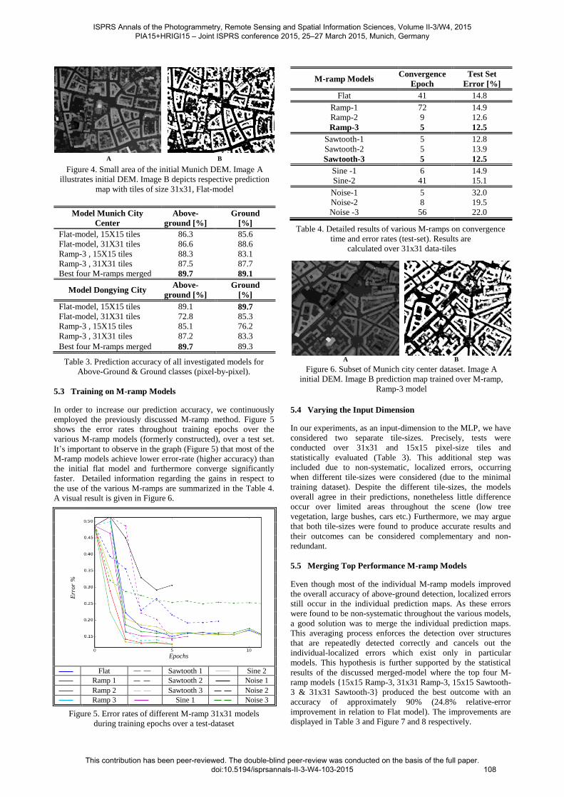
Figure 4. Small area of the initial Munich DEM. Image A

illustrates initial DEM. Image B depicts respective prediction

map with tiles of size 31x31, Flat-model

Model Munich City

Center

Above-

ground [%]

Ground

[%]

Flat-model, 15X15 tiles 86.3 85.6


Ramp-3 , 15X15 tiles 88.3 83.1

Ramp-3 , 31X31 tiles 87.5 87.7

Best four M-ramps merged 89.7 89.1

Model Dongying City Above-

ground [%]

Ground

[%]



Ramp-3 , 15X15 tiles 85.1 76.2

Ramp-3 , 31X31 tiles 87.2 83.3

Best four M-ramps merged 89.7 89.3

Table 3. Prediction accuracy of all investigated models for

Above-Ground & Ground classes (pixel-by-pixel).

5.3 Training on M-ramp Models

In order to increase our prediction accuracy, we continuously

employed the previously discussed M-ramp method. Figure 5

shows the error rates throughout training epochs over the

various M-ramp models (formerly constructed), over a test set.

It’s important to observe in the graph (Figure 5) that most of the

M-ramp models achieve lower error-rate (higher accuracy) than

the initial flat model and furthermore converge significantly

faster. Detailed information regarding the gains in respect to

the use of the various M-ramps are summarized in the Table 4.

A visual result is given in Figure 6.

Err

or

%

Epochs

Flat Sawtooth 1 Sine 2

Ramp 1 Sawtooth 2 Noise 1

Ramp 2 Sawtooth 3 Noise 2

Ramp 3 Sine 1 Noise 3

Figure 5. Error rates of different M-ramp 31x31 models

during training epochs over a test-dataset

M-ramp Models Convergence

Epoch

Test Set

Error [%]

Flat 41 14.8

Ramp-1 72 14.9

Ramp-2 9 12.6

Ramp-3 5 12.5

Sawtooth-1 5 12.8

Sawtooth-2 5 13.9

Sawtooth-3 5 12.5

Sine -1 6 14.9

Sine-2 41 15.1

Noise-1 5 32.0

Noise-2 8 19.5

Noise -3 56 22.0

Table 4. Detailed results of various M-ramps on convergence

time and error rates (test-set). Results are

calculated over 31x31 data-tiles

3 1

A B

Figure 6. Subset of Munich city center dataset. Image A

initial DEM. Image B prediction map trained over M-ramp,

Ramp-3 model

5.4 Varying the Input Dimension

In our experiments, as an input-dimension to the MLP, we have

considered two separate tile-sizes. Precisely, tests were

conducted over 31x31 and 15x15 pixel-size tiles and

statistically evaluated (Table 3). This additional step was

included due to non-systematic, localized errors, occurring

when different tile-sizes were considered (due to the minimal

training dataset). Despite the different tile-sizes, the models

overall agree in their predictions, nonetheless little difference

occur over limited areas throughout the scene (low tree

vegetation, large bushes, cars etc.) Furthermore, we may argue

that both tile-sizes were found to produce accurate results and

their outcomes can be considered complementary and non-

redundant.

5.5 Merging Top Performance M-ramp Models

Even though most of the individual M-ramp models improved

the overall accuracy of above-ground detection, localized errors

still occur in the individual prediction maps. As these errors

were found to be non-systematic throughout the various models,

a good solution was to merge the individual prediction maps.

This averaging process enforces the detection over structures

that are repeatedly detected correctly and cancels out the

individual-localized errors which exist only in particular

models. This hypothesis is further supported by the statistical

results of the discussed merged-model where the top four M-

ramp models {15x15 Ramp-3, 31x31 Ramp-3, 15x15 Sawtooth-

3 & 31x31 Sawtooth-3} produced the best outcome with an

accuracy of approximately 90% (24.8% relative-error

improvement in relation to Flat model). The improvements are

displayed in Table 3 and Figure 7 and 8 respectively.



108

3 1

A B

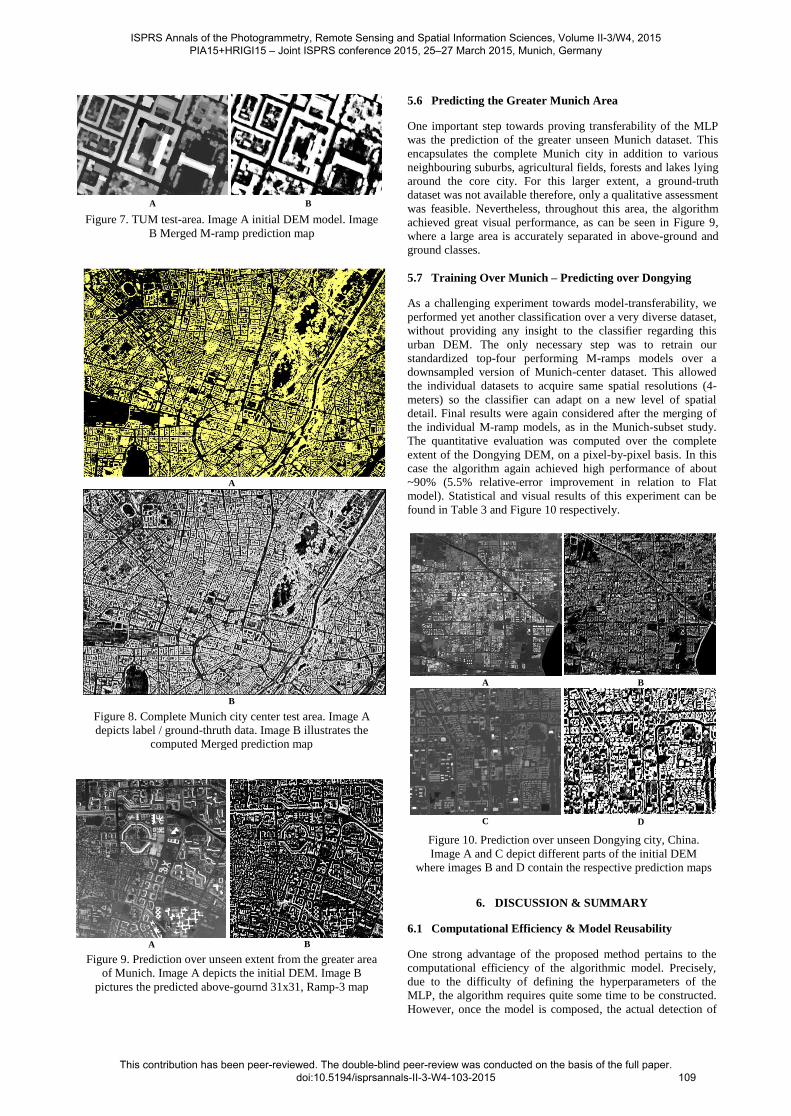
Figure 7. TUM test-area. Image A initial DEM model. Image

B Merged M-ramp prediction map

A

B

Figure 8. Complete Munich city center test area. Image A

depicts label / ground-thruth data. Image B illustrates the

computed Merged prediction map

A B

Figure 9. Prediction over unseen extent from the greater area

of Munich. Image A depicts the initial DEM. Image B

pictures the predicted above-gournd 31x31, Ramp-3 map

5.6 Predicting the Greater Munich Area

One important step towards proving transferability of the MLP

was the prediction of the greater unseen Munich dataset. This

encapsulates the complete Munich city in addition to various

neighbouring suburbs, agricultural fields, forests and lakes lying

around the core city. For this larger extent, a ground-truth

dataset was not available therefore, only a qualitative assessment

was feasible. Nevertheless, throughout this area, the algorithm

achieved great visual performance, as can be seen in Figure 9,

where a large area is accurately separated in above-ground and

ground classes.

5.7 Training Over Munich – Predicting over Dongying

As a challenging experiment towards model-transferability, we

performed yet another classification over a very diverse dataset,

without providing any insight to the classifier regarding this

urban DEM. The only necessary step was to retrain our

standardized top-four performing M-ramps models over a

downsampled version of Munich-center dataset. This allowed

the individual datasets to acquire same spatial resolutions (4-

meters) so the classifier can adapt on a new level of spatial

detail. Final results were again considered after the merging of

the individual M-ramp models, as in the Munich-subset study.

The quantitative evaluation was computed over the complete

extent of the Dongying DEM, on a pixel-by-pixel basis. In this

case the algorithm again achieved high performance of about

~90% (5.5% relative-error improvement in relation to Flat

model). Statistical and visual results of this experiment can be

found in Table 3 and Figure 10 respectively.

A B

C

D

Figure 10. Prediction over unseen Dongying city, China.

Image A and C depict different parts of the initial DEM

where images B and D contain the respective prediction maps

6. DISCUSSION & SUMMARY

6.1 Computational Efficiency & Model Reusability

One strong advantage of the proposed method pertains to the

computational efficiency of the algorithmic model. Precisely,

due to the difficulty of defining the hyperparameters of the

MLP, the algorithm requires quite some time to be constructed.

However, once the model is composed, the actual detection of



109

the above-ground objects concludes in just a few minutes.

Furthermore, through a series of experiments, we provided

evidence regarding the transferability of the model without the

need of re-training the system (for data with same spatial

resolution). This key aspect further supports the potential re-

usability of DL classifiers in the context of above-ground

detection.

6.2 Remarks on M-ramp

Even though our experiments suggest that M-ramp can

generally improve the above-ground object detection within the

urban extent, it is important for one to understand the

limitations imposed by the classification algorithm prior to

using it. M-ramp can improve DEM classification as long as the

algorithm has a large enough capacity to accurately detect and

model all variations contained within the training data and still

have enough potential left to compensate for the information

introduced by the M-ramp method. Therefore providing

extensively altered relief to a strongly restricted / regularized

classifier may result in a decrease in classification accuracy.

Such a case is visible in Figure 5 where the white-noise models

clearly drop in overall accuracy. Nonetheless, despite this

decline the majority of the other M-ramps significantly

enhanced model correctness and convergence time. All the

above facts establish M-ramp as an additional regularizer in the

context of DL and DEM classification and suggests that their

engaging properties should be further investigated in future

studies.

6.3 Remarks over Classification Accuracies

Even though the accuracies we have acquired in the task of

above-ground object detection were quite high, we strongly

believe that the actual predictions are more precise than

statistically presented. Considering the error rate of the labels

lying around 7%, one can understand the significant impact they

result over our final error estimation. This argument can be

further supported by visual comparison where the prediction

maps state the truth and the labels are wrong. In addition, a

separation in ground and above-ground classes over a

label/ground-truth dataset is a non-trivial and quite subjective

task due to the existence of multiple objects that could

potentially belong to either class (bushes, cars, large rock

formations, etc.)

6.4 Summary

In this work, we presented a generic framework for above-

ground object detection using MLP over a raw DEM model. We

have showed that even by extensively shrinking the training

dataset, we can still achieve very good performance and even

re-use the classifier over different unseen datasets. Additionally,

we introduced a new method, called M-ramp which

significantly improves performance and convergence time.

These aspects clearly highlight the potentials of DL in the field

of remote sensing and we hope that our work will inspire

researchers in the field to implement these techniques to

accomplish new milestones.

As future implementations of DL in DEM object extraction,

we would be interested in trying to separate between building-

structures and vegetation by again using raw DEM data.

Additionally, in the same context, the implementation of

different DL models such as Convolutional Neural Networks

and Deep Belief Network would be also of great interest.

REFERENCES

Baillard, C., Maıtre, H., 1999. 3D reconstruction of urban

scenes from aerial stereo imagery: a focusing strategy.

Computer Vision and Image Understanding, 76(3), pp. 244-258.

Belli, T., Cord, M., Jordan, M., 2001. 3D Data reconstruction

and modeling for urban scene analysis. In Workshop of

Automatic Extraction of Man-made Objects from Aerial and

Satellite Images, A.A. Balkema Publishers, (3), pp. 125-134.

Dalal, N., Triggs, B., 2005. Histograms of oriented gradients for

human detection. In IEEE Conference on Computer Vision and

Pattern Recognition 2005, (1), pp. 886–893.

Marconcini, M., Marmanis, D., Esch, T., Felbier, A., 2014. A

novel method for building height estimation using TanDEM-X

data. In IEEE International Geoscience and Remote Sensing

Symposium (IGARSS), 2014, pp. 4804-4807.

Ortner, M., Descombes, X., Zerubia, J., 2007. Building outline

extraction from digital elevation models using marked point

processes. International Journal of Computer Vision, 72(2), pp.

107-132.

Rosenblatt, F., 1957. The Perceptron - a perceiving and

recognizing automaton. Report 85-460-1, Cornell Aeronautical

Laboratory.

Rumelhart, D., Hinton, G., Williams, R., 1986. Learning

representations by back-propagating errors. Nature 323, pp.

533-536.

Sirmacek, B., & Unsalan, C., 2009. Urban-area and building

detection using SIFT keypoints and graph theory. In IEEE

Transactions on Geoscience and Remote Sensing, 47(4), pp.

1156-1167.

Srebro, N., Shraibman A., 2005. Rank, trace-norm and max-

norm. In Proceedings of the 18th annual conference on

Learning Theory (COLT) 2005, pp. 545-560.

Srivastava, N., Hinton, G., Krizhevsky, A., Sutskever, I.,

Salakhutdinov, R., 2014. Dropout: A simple way to prevent

neural networks from overfitting. The Journal of Machine

Learning Research, 15(1), pp. 1929-1958.

Tournaire, O., Bredif, M., Boldo, D., Durupt, M., 2010. An

efficient stochastic approach for building footprint extraction

from digital elevation models. ISPRS Journal of

Photogrammetry and Remote Sensing, 65(4), pp. 317-327.

Vincent, P., Larochelle, H., Bengio, Y., Manzagol, P., 2008.

Extracting and composing robust features with denoising

autoencoders. In Proceedings of the 25th International

Conference on Machine Learning, pp. 1096-1103.

Zingaretti, P., Frontoni, E., Forlani, G., Nardinocchi, C., 2007.

Automatic extraction of LIDAR data classification rules. In

14th International Conference on Image Analysis and

Processing (ICIAP) 2007, pp. 273-278.



110

http://scholar.google.com/scholar?oi=bibs&hl=en&cluster=7817802389471101066&btnI=1

http://scholar.google.com/scholar?oi=bibs&hl=en&cluster=7817802389471101066&btnI=1

Documents

DEEP NEURAL NETWORKS FOR ABOVE-GROUND DETECTION IN …