Deep Relative Geologic Time: A Deep Learning Method for

1. IntroductionSeismic horizon interpretation is common and critical in seismic interpretation for building subsurface structural and stratigraphic models and usually helps the analysis of seismic geomorphology (Mitchum et al., 1977; Posamentier et al., 2007). By laterally tracking seismic reflections, we can manually identify horizons because they are considered as geologically synchronous surfaces. Different approaches have been proposed to automatically or semi-automatically extract horizons from seismic image volumes by tracking

Abstract Extracting horizons and detecting faults in a seismic image are basic steps for structural interpretation and important for many seismic processing schemes. A common ground of the two tasks is to analyze seismic structures and they are related to each other. However, previously proposed methods deal with the tasks independently, and challenge remains in each of them. We propose a volume-to-volume neural network to estimate a relative geologic time (RGT) volume from a seismic volume, and this RGT volume is further used to simultaneously interpret horizons and faults. The network uses U-shaped framework with attention mechanism to systematically aggregate multi-scale information and automatically highlight informative features, and achieves high prediction accuracy with affordable computational costs. To train the network, we build thousands of 3-D noisy synthetic seismic volumes and corresponding RGT volumes with realistic and various structures. We introduce a loss function based on structure similarity to capture spatial dependencies among seismic samples for better optimizing the network, and use multiple reasonable assessments to evaluate the predicted results. Trained by using synthetic data, our network outperforms the conventional approaches in recognizing structural features in field data examples. Once obtaining an RGT volume, we can not only obtain seismic horizons by simply extracting RGT constant surfaces but also detect faults that are indicated by lateral RGT discontinuities. To be able to deal with large seismic volumes, we further propose a workflow to first estimate sub-volumes of RGT and merge them to obtain a full RGT volume without boundary artifacts.

Plain Language Summary We propose a volume-to-volume deep network to accurately compute an RGT volume from the seismic image volume without any manual picking constraints, which is further used to simultaneously interpret horizons and faults. This network is simplified from the originally more complicated UNet and supplemented by multi-scale residual learning and attention mechanisms to achieve acceptable computational costs but still preserve the high prediction accuracy for RGT estimation. We use a non-trivial criterion based on structural similarity to optimize the network parameters. We train the network by using synthetic data, which are automatically generated by adding folding and faulting structures to an initial flat seismic and RGT volumes. Our CNN model not only shows promising prediction performance on the synthetic data excluded in training but also works well in the multiple field seismic volumes that are recorded at totally different surveys to reliably capture complex structural features such as crossing faults and complicatedly folded horizons. The applications in the three field data examples demonstrate the prediction performance and reliable generalization ability of the trained CNN model. These results can provide valuable information by revealing complex subsurface structures, which is of importance to many human activities ranging from natural source exploration to geothermal energy production.

BI ET AL.

© 2021. American Geophysical Union. All Rights Reserved.

Deep Relative Geologic Time: A Deep Learning Method for Simultaneously Interpreting 3-D Seismic Horizons and FaultsZhengfa Bi1, Xinming Wu1 , Zhicheng Geng2 , and Haishan Li3

1School of Earth and Space Sciences, University of Science and Technology of China, Hefei, China, 2Bureau of Economic Geology, University of Texas at Austin, Austin, TX, USA, 3Research Institute of Petroleum Exploration and Development-Northwest (NWGI), Lanzhou, China

Key Points:• We propose an encoder-decoder

network with attention mechanism to estimate relative geologic time (RGT) volumes from 3D seismic images

• We train the network with a criterion of structural similarity which enables the network capture seismic structural interdependences

• Our method can deal with large 3D seismic images and estimate RGT volumes from which all horizons and faults can be automatically extracted

Correspondence to:X. Wu,[email protected]

Citation:Bi, Z., Wu, X., Geng, Z., & Li, H. (2021). Deep relative geologic time: A deep learning method for simultaneously interpreting 3-D seismic horizons and faults. Journal of Geophysical Research: Solid Earth, 126, e2021JB021882. https://doi.org/10.1029/2021JB021882

Received 14 FEB 2021Accepted 20 AUG 2021

10.1029/2021JB021882

Special Section:Machine learning for Solid Earth observation, modeling and understanding

RESEARCH ARTICLE

1 of 24

https://orcid.org/0000-0002-4910-8253

https://orcid.org/0000-0002-0482-4459

https://doi.org/10.1029/2021JB021882

http://agupubs.onlinelibrary.wiley.com/doi/toc/10.1002/(ISSN)2169-9356.MACHLRN1



http://crossmark.crossref.org/dialog/?doi=10.1029%2F2021JB021882&domain=pdf&date_stamp=2021-09-12

Journal of Geophysical Research: Solid Earth

BI ET AL.

10.1029/2021JB021882

2 of 24

constant seismic instantaneous phases (Lou et al., 2020; Stark, 2003; X. Wu & Zhong, 2012), classifying seis-mic waveforms (Figueiredo et al., 2015; H. Wu et al., 2019), or following geometric orientations of seismic reflections (Bakker, 2002; Lomask et al., 2006; Parks, 2010; Monniron et al., 2016; X. Wu & Hale, 2015; X. Wu & Fomel, 2018b; Zinck et al., 2013). Although these horizon extraction methods can honor laterally coherent reflections, they are often sensitive to structural and stratigraphic discontinuities and usually has difficulties in correctly correlating horizons dislocated by faults. To overcome this problem, some methods introduce prior identification of faults and remove them from seismic images before tracking horizons (Luo & Hale, 2013; X. Wu et al., 2016), which demonstrates that the implementation of fault constraints signifi-cantly improve the accuracy and reliability of the horizon tracking process.

Faults are another type of geologically significant structures that control the boundaries of seismic horizons and helps to reduce well placement risk in reservoir exploration. In a seismic image, faults are typically indicated by lateral reflection discontinuities. Based on this observation, numerous fault detection methods compute a set of additional attribute images such as semblance (Marfurt et al., 1998), coherency (Karimi et al., 2015; Li & Lu, 2014; Marfurt et al., 1999), variance (Van Bemmel & Pepper, 2000), curvature (Al-Dos-sary & Marfurt, 2006; Di & Gao, 2016; Roberts, 2001), or fault likelihood (Hale, 2013), where fault features are enhanced while other structural and stratigraphic features are suppressed. In calculating these fault attributes, we often need to estimate reflection slopes and measure reflection discontinuities along seismic horizons (Gersztenkorn & Marfurt, 1999; Hale, 2009, 2013; Karimi et al., 2015). However, the computed attributes are typically sensitive to noisy or stratigraphic features that are apparent to be discontinuities, which causes the necessity of using extra processing such as ant tracking (Pedersen et al., 2003) and optimal surface voting (X. Wu & Fomel, 2018a) to further highlight fault-related features. Di et al. (2020) propose to use interpreted horizons as structural constraints to compute a more reliable fault detection map. To further estimate fault displacements, horizons across faults are required to be manually picked (Duffy et al., 2015; Reeve et al., 2015) or automatically correlated (Hale, 2012; Liang et al., 2010).

Based on the above discussions, the two tasks of interpreting seismic horizons and faults are related to each other as interpreting horizons across faults often requires first picking faults to provide a boundary control while computing a reliable fault map and estimating fault displacements typically requires first interpreting horizons across faults. However, most of the previously proposed methods deal with the two tasks independently and further improvements to each task are feasible and worthwhile. In this study, we propose to simultaneously interpret 3-D seismic horizons and faults by computing a relative geologic time (RGT) volume (Stark, 2004, 2005a, 2005b, 2006) from 3-D seismic volume by using deep learning. In an RGT volume, each data sample is assigned a geologic time value corresponding to the reflection amplitude in seismic volume. Its RGT contours indicate a set of geologically synchronous surfaces that represent seis-mic horizons, which enables RGT volume store rich geometrical relations of all sorts of geologic structures. For this reason, some relevant discontinuous features such as faults and unconformities are also implicitly embedded and enhanced by sharp structural edges in an RGT volume. An accurate RGT volume is thus helpful to well understand geologic structures of interest and qualify reservoir properties of continuity and morphology to interpret all associated geologic structures, and to build a subsurface model of a particular environment. It has shown great promise in many applications to improve horizon extraction (Stark, 2004; Fomel, 2010; X. Wu & Zhong, 2012), sedimentologic interpretation (Hongliu et al., 2012), stratigraphic in-terpretation (Alliez et al., 2007; Karimi & Fomel, 2015; Lacaze et al., 2017), geologic body detection (Prazuck et al., 2015), and structural implicit modeling (Grose et al., 2017; Irakarama et al., 2020; Laurent et al., 2016; Renaudeau et al., 2019).

A straightforward but laborious way of estimating RGTs is to automatically track or manually pick seismic horizons as many as possible and then assign every horizon surface an RGT value. With the known time values, we can interpolate the values elsewhere. However, although the resulting RGT volume strictly hon-ors the interpreted horizons, it fails in resolving local structures among these horizons and its accuracy is usually subject to the precision of horizon picking methods. To improve the RGT estimation, the phase un-wrapping method (Stark, 2003; X. Wu & Zhong, 2012) has been proposed to calculate RGT volume by using the instantaneous phase information computed from seismic traces. Also, an RGT volume can be estimated from the slopes of seismic reflections computed by using the plane-wave-destruction method (Fomel, 2002).


BI ET AL.

10.1029/2021JB021882

3 of 24

Although those slope-based methods can correctly capture local structural features and consistently follow laterally continuous reflections, they cannot track reflections significantly displaced across faults.

Deep learning (LeCun et al., 2015; Goodfellow et al., 2016) is a data-driven system that derives a mapping function between inputs and outputs from example data or past experiences without any prior knowledge of physical theories. In many learning algorithms, supervised learning is essential due to its ability to cap-ture highly complex and strongly nonlinear relationships by extracting general representation and knowl-edge from the training data set (Kappler et al., 2005). Because of many successful applications in natural image processing tasks (Badrinarayanan et al., 2017; Chen et al., 2014, 2017; Ciregan et al., 2012; Krizhevsky et al., 2012), deep learning methods have recently been introduced to deal with geophysical problems, such as channel interpretation (Pham et al., 2019; H. Gao et al., 2020), salt body detection (Sen et al., 2020; Shi et al., 2019), fault detection (Xiong et al., 2018; X. Wu, Liang, Shi, & Fomel, 2019), waveform inversion (Y. Wu & McMechan, 2019; Yang & Ma, 2019; Q. He & Wang, 2021), and noise attenuation (Yu et al., 2019).

Recently, Geng et al. (2020) demonstrate that the U-shaped architectures designed for natural image seg-mentation can be successfully repurposed for a 2-D RGT estimation task. This network is designed to pro-gressively extract highly abstractive presentations and knowledge of the seismic images by dealing with multi-scale spatial features. Through such a sequential process, the outputs are conditioned on informa-tion collected from a large receptive field to robustly fit the RGT images. To improve the representational power of the CNN, they propose a very deep network by using successive residual learning blocks in the encoder and decoder branches. Although network depth is considered to be of central importance for many Computer Vision issues (K. He et al., 2016; Laina et al., 2016), simply stacking residual blocks to form a deeper network can hardly obtain better improvements. For example, the excessive use of down-sampling generates extremely small-size feature maps where the structural information is hardly preserved, and thus hinders the following learning units to accurately construct the seismic structures again in the predictions. Also, a deeper network is typically more difficult to train and limited to the 3-D seismic processing because the computation times soon become unaffordable. Thus, whether a more complex network positively con-tributes to RGT estimation or not and how to construct a trainable deep network remains to be studied. In addition, without discriminative learning ability, this network treats each channel-wise feature equally and might not appropriately focus on geologic structures with varying shapes and sizes. On the other hand, the conventional point-wise loss function used by Geng et al. (2020) cannot correctly distinguish structural differences between targets and predictions.

We propose a simplified 3-D deep network with encoder-decoder architecture and attention mechanism to produce point-wise predictions of RGT from seismic amplitude volume to achieve accurate structural interpretation at cost of affordable computations. For a variety of natural image processing tasks in which inputs are mapped to outputs with the same resolution, the encoder-decoder framework is considered as a standard design principle because of its excellent performance and efficiency. These advantages are significantly related to the systematic aggregation of information at multiple spatial scales by repeatedly down-sampling features and using multiple skip connections. The up-sampled features that capture coarse variations of seismic amplitudes can be channel-wisely concatenated with their up-sampled counterparts to capture detailed patterns and preserve spatial resolutions. Based on this architecture, we introduce an atten-tion mechanism to enable the network automatically learn to suppress irrelevant features while enhancing informative ones for achieving accurate predictions.

The RGT estimation task involves the analysis of seismic structures that are characterized by the variations of amplitude distributions, in which one image sample is associated with the others, but an individual seis-mic sample is usually not important for structural interpretation. According to this observation, commonly used point-wise criterion in regression problems such as MSE (mean square error) might not correctly dis-tinguish structural patterns between predictions and targets. To solve this problem, we use a loss function based on structural similarity to train our network, such that it can explicitly learn spatial interdependen-cies among different seismic samples instead of just approximating each single RGT value.

Although deep learning has shown its promising ability in capturing complexly non-linear relations, it is typically based on tremendous amounts of labeled data. In many other tasks where deep learning has obtained significant successes, such as natural image classification (Krizhevsky et al., 2012; Simonyan


BI ET AL.

10.1029/2021JB021882

4 of 24

et al., 2013) and segmentation (Badrinarayanan et al., 2017; Chen et al., 2017), the training data have been well prepared. In most geophysical problems including the RGT estimation, it is tedious and error-prone to completely label all the data in a particular field seismic survey (X. Wu, Liang, Shi, Geng, & Fomel, 2019). To address this problem, we develop a workflow to obtain a tremendous amount of training data with realistic and varying structures and correct geologic labels (RGT volumes), which are all automatically created by sequentially performing folding and faulting transformations and adding random noise.

Once estimating an RGT volume, we are able to simultaneously interpret different types of geological struc-tures in the seismic volumes. For example, we show how to extract seismic horizons by simply following a set of constant RGT isovalues and accurately detect faults through the same network that takes the seismic and RGT volumes as inputs to produce a fault detection image as their features are highlighted by sharp edges. By using three field data examples, we demonstrate that the network trained by using the synthetic data can be successfully applied to recognize general structural patterns. To further generalize our method to a real seismic data volume larger then the training samples, we develop a workflow to merge the predict-ed sub-volumes to obtain a full RGT volume covering the whole seismic amplitudes.

2. MethodIn this section, we use a volume-to-volume deep neural network with a U-shaped framework supplement-ed by multi-scale residual learning and attention mechanisms to recognize structural patterns from a 3-D seismic image and estimate the corresponding RGT volume. For properly training the network, a quality assessment based on structural similarity is employed as a loss function to optimize the model parameters within each epoch. In addition, a variety of quality measurements are proposed to evaluate the predicted results and demonstrate the effectiveness of our approach.

2.1. Network Architecture

The architecture of our network is based on UNet (Ronneberger et al., 2015) that has been commonly used for many image segmentation tasks due to its excellent performance and efficient use of GPU memory. Its great representational power is related to the extraction of image features at multi-scales in a gradual manner. In this network, the inputs are mapped to outputs of the same resolution, where the features are down-sampled in the encoder and later combined with their up-sampled counterparts through channel concatenation. However, the almost complete elimination of spatial resolutions preserves little structural information in the extremely small-size features and hinders the decoder from correctly identifying seismic structures. This might not be important in tasks of nature image classification, where a single object often dominates the images, but would play a significant role in the structural analysis task, in which horizons or faults and their relative configurations should be taken into consideration.

In addition to the spatial resolution, computational cost control is also essential in the 3-D seismic pro-cessing task. The conventional learning-based methods use multi-stage cascaded convolutional neural net-works (CNNs) to achieve their excellent representational power, which often introduces a large number of model parameters and produces prohibitive computational costs especially in dealing with high-dimen-sional seismic data. Thus, how to accurately and efficiently capture complex 3-D seismic structures poses a new challenge beyond the capability of the currently existing two-dimensional structural interpretation methods. To solve this problem, we propose a CNN model that can automatically learn to estimate the RGT volumes from the corresponding 3-D seismic images with varying and complex structural patterns.

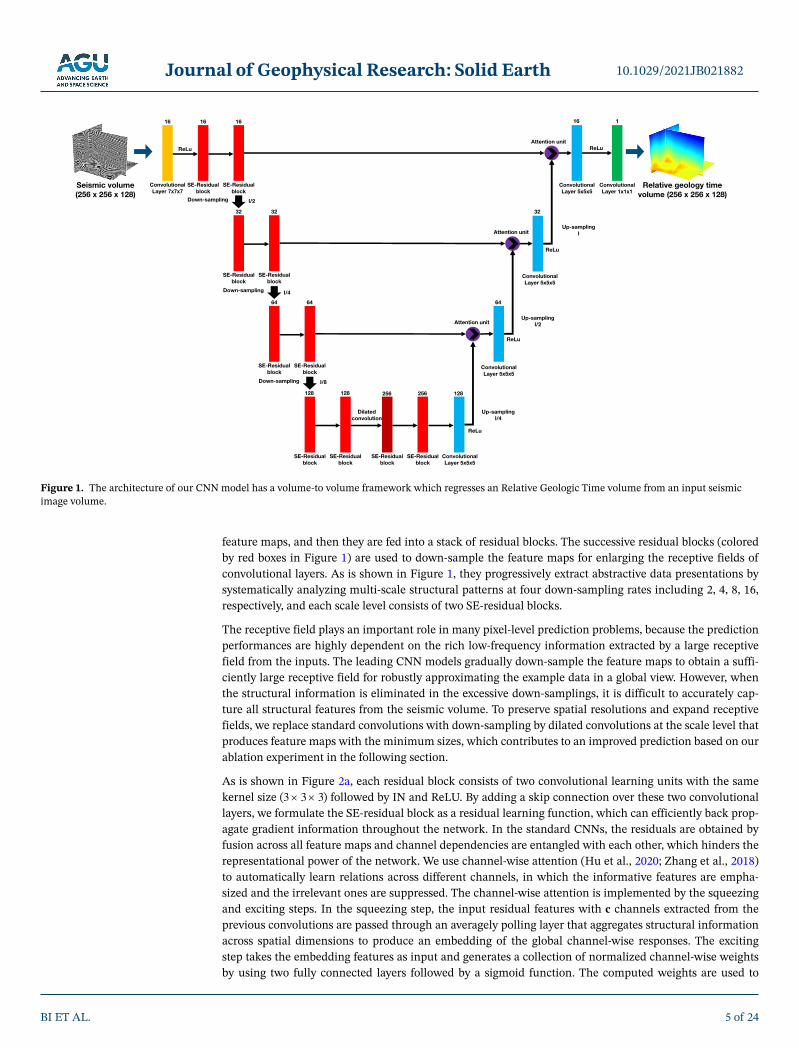
Our network (Figure 1) is simplified and modified from an encoder-decoder architecture of UNet. This net-work uses skip connections to achieve multi-scale aggregation by systematically combining the high-level semantic features from the decoder and corresponding low-level detailed features from the encoder. Such a multi-scale structural analysis contributes to not only accurate predictions but also improved computation-al efficiency because the down-sampling steps can compress the intermediate feature maps to save com-putational costs. In our network, the encoder branch consists of 21 convolutional layers to systematically aggregate multi-scale structural features, starting from a 7 7 7E convolution layer followed by Instance Normalization (IN) (Ulyanov et al., 2016) and Rectified Linear Unit (ReLu) (Nair & Hinton, 2010). The first convolutional layer takes the input seismic volume and computes 16 local, translational invariant low-level


BI ET AL.

10.1029/2021JB021882

5 of 24

feature maps, and then they are fed into a stack of residual blocks. The successive residual blocks (colored by red boxes in Figure 1) are used to down-sample the feature maps for enlarging the receptive fields of convolutional layers. As is shown in Figure 1, they progressively extract abstractive data presentations by systematically analyzing multi-scale structural patterns at four down-sampling rates including 2, 4, 8, 16, respectively, and each scale level consists of two SE-residual blocks.

The receptive field plays an important role in many pixel-level prediction problems, because the prediction performances are highly dependent on the rich low-frequency information extracted by a large receptive field from the inputs. The leading CNN models gradually down-sample the feature maps to obtain a suffi-ciently large receptive field for robustly approximating the example data in a global view. However, when the structural information is eliminated in the excessive down-samplings, it is difficult to accurately cap-ture all structural features from the seismic volume. To preserve spatial resolutions and expand receptive fields, we replace standard convolutions with down-sampling by dilated convolutions at the scale level that produces feature maps with the minimum sizes, which contributes to an improved prediction based on our ablation experiment in the following section.

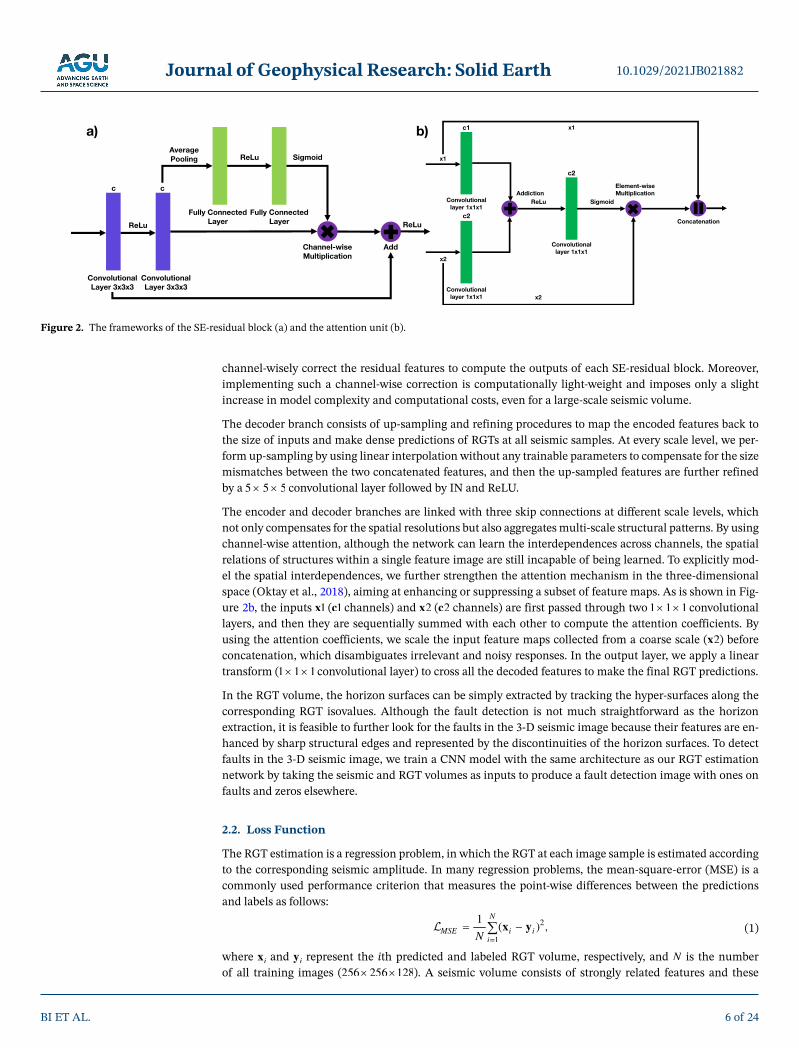
As is shown in Figure 2a, each residual block consists of two convolutional learning units with the same kernel size (3 3 3E ) followed by IN and ReLU. By adding a skip connection over these two convolutional layers, we formulate the SE-residual block as a residual learning function, which can efficiently back prop-agate gradient information throughout the network. In the standard CNNs, the residuals are obtained by fusion across all feature maps and channel dependencies are entangled with each other, which hinders the representational power of the network. We use channel-wise attention (Hu et al., 2020; Zhang et al., 2018) to automatically learn relations across different channels, in which the informative features are empha-sized and the irrelevant ones are suppressed. The channel-wise attention is implemented by the squeezing and exciting steps. In the squeezing step, the input residual features with E c channels extracted from the previous convolutions are passed through an averagely polling layer that aggregates structural information across spatial dimensions to produce an embedding of the global channel-wise responses. The exciting step takes the embedding features as input and generates a collection of normalized channel-wise weights by using two fully connected layers followed by a sigmoid function. The computed weights are used to

Figure 1. The architecture of our CNN model has a volume-to volume framework which regresses an Relative Geologic Time volume from an input seismic image volume.

Seismic volume (256 x 256 x 128)

Relative geology time volume (256 x 256 x 128)

16

ConvolutionalLayer 7x7x7

SE-Residual block

SE-Residual block

16 16

SE-Residual block

SE-Residual block

32 32

Down-sampling

SE-Residual block

SE-Residual block

64 64

Down-sampling

SE-Residual block

SE-Residual block

128 128

Down-sampling

I/2

I/4

I/8

SE-Residual block

SE-Residual block

256 256

Dilated convolution

128

64

32

Up-samplingI/4

Up-samplingI/2

Up-samplingI

16





1


Attention unit

Attention unit

Attention unitReLu

ReLu

ReLu

ReLu

ReLu


BI ET AL.

10.1029/2021JB021882

6 of 24

channel-wisely correct the residual features to compute the outputs of each SE-residual block. Moreover, implementing such a channel-wise correction is computationally light-weight and imposes only a slight increase in model complexity and computational costs, even for a large-scale seismic volume.

The decoder branch consists of up-sampling and refining procedures to map the encoded features back to the size of inputs and make dense predictions of RGTs at all seismic samples. At every scale level, we per-form up-sampling by using linear interpolation without any trainable parameters to compensate for the size mismatches between the two concatenated features, and then the up-sampled features are further refined by a 5 5 5E convolutional layer followed by IN and ReLU.

The encoder and decoder branches are linked with three skip connections at different scale levels, which not only compensates for the spatial resolutions but also aggregates multi-scale structural patterns. By using channel-wise attention, although the network can learn the interdependences across channels, the spatial relations of structures within a single feature image are still incapable of being learned. To explicitly mod-el the spatial interdependences, we further strengthen the attention mechanism in the three-dimensional space (Oktay et al., 2018), aiming at enhancing or suppressing a subset of feature maps. As is shown in Fig-ure 2b, the inputs 1E x ( 1E c channels) and 2E x ( 2E c channels) are first passed through two 1 1 1E convolutional layers, and then they are sequentially summed with each other to compute the attention coefficients. By using the attention coefficients, we scale the input feature maps collected from a coarse scale ( 2E x ) before concatenation, which disambiguates irrelevant and noisy responses. In the output layer, we apply a linear transform (1 1 1E convolutional layer) to cross all the decoded features to make the final RGT predictions.

In the RGT volume, the horizon surfaces can be simply extracted by tracking the hyper-surfaces along the corresponding RGT isovalues. Although the fault detection is not much straightforward as the horizon extraction, it is feasible to further look for the faults in the 3-D seismic image because their features are en-hanced by sharp structural edges and represented by the discontinuities of the horizon surfaces. To detect faults in the 3-D seismic image, we train a CNN model with the same architecture as our RGT estimation network by taking the seismic and RGT volumes as inputs to produce a fault detection image with ones on faults and zeros elsewhere.

2.2. Loss Function

The RGT estimation is a regression problem, in which the RGT at each image sample is estimated according to the corresponding seismic amplitude. In many regression problems, the mean-square-error (MSE) is a commonly used performance criterion that measures the point-wise differences between the predictions and labels as follows:

2

1

1 ( ) ,N

MSE i iiN

x y (1)

where iE x and iE y represent the ith predicted and labeled RGT volume, respectively, and E N is the number of all training images (256 256 128E ). A seismic volume consists of strongly related features and these

Figure 2. The frameworks of the SE-residual block (a) and the attention unit (b).

a) b)

Convolutionallayer 1x1x1

c2


c1


ReLu Sigmoid

c2

x1

x2

x1

x2

Concatenation

AddictionElement-wise Multiplication

c c

Average Pooling



Fully Connected Layer

SigmoidReLu

Channel-wise Multiplication

Add

Fully Connected LayerReLu ReLu


BI ET AL.

10.1029/2021JB021882

7 of 24

dependencies exist in the seismic amplitude distribution carrying spatial information of geological struc-tures. Generally, the MSE has the advantages of speeding up the optimization and producing a stable solution, but it might not be appropriate to characterize the structural errors, especially for the associated structures such as the faults and reflections. For example, when all seismic horizons have been correctly interpreted, the faults can be simply considered as the discontinuities across numerous horizons. Because the point-wise measurement such as MSE or MAE is not sufficient to correctly represent these relations, the two RGT volumes with similar MSE might appear significantly different structures.

To properly measure the structural errors for our RGT estimation, we use the performance criterion based on structural similarity (SSIM) (Wang et al., 2004; Zeng & Wang, 2012) as the loss function. The SSIM is originally proposed as a complementary framework based on the degradation of nature image structures to quantify the visibility of errors between distorted images and reference ones, which has shown great performance in a variety of Computer Vision tasks. In our problem, we formulate the SSIM in a 3-D case as follows:

1 22 2 2 2

1 2

(2 )(2 ),

( )( )SSIMC C

C C

x y xy

x y x y (2)

where two small constant factors 1E C and 2E C are added to avoid the numerical calculation unstable when denominator of 2 is close to zero. In this experiment, 2

1 1( )E C k L and 22 ( 2 )E C k L are set according to

(Wang et al., 2003), in which 1 0.01E k and 2 0.03E k are two constant scalars, and 5E L is determined by the average dynamic range of the RGT volumes of our training data set. The structural similarity is evaluated from three aspects, including mean values E , standard deviations E , and covariances E xy for the two RGT volumes. To estimate the SSIM, we first construct a 3-D Gaussian window with a size of 11 11 11E samples. Then we point-wisely move this widow and evaluate the corresponding local structural similarity degree for each slide according to Equation 2, to compute SSIM coefficients for all the image samples. We calculate the structural similarity for the overall RGT volumes between predicted and target RGT volumes by averaging these local SSIM coefficients. In this way, the estimated SSIM reaches its best value at 1 only for two identi-cal RGT volumes, and represents perfect structural similarity. Contrarily, an SSIM value of 0 represents little structural similarity. Therefore, we minimize the following loss objective to optimize the RGT prediction performance in training:

Rgt SSIM 1 . (3)

The fault detection can be considered as a binary segmentation problem, which takes both seismic image and RGT volume as inputs to produce a detection map with ones at fault positions and zeros elsewhere on the seismic sampling grid. For the conventional image segmentation problem, the cross-entropy is com-monly used in the loss function, which can be written as follow:

1 1log( ) (1 ) log(1 ),

N N

Fault i i i ii i

y x y x (4)

where E N denotes the number of all samples in the seismic image. The term iE y represents the ground truth of binary labels and iE x represents the probabilities that are computed from the sigmoid activation of the network predictions. Because the true labels iE y are binary values, the first term measures the prediction er-rors at the fault samples, whereas the second term measures the prediction errors at the non-fault samples.

This loss function works well in most binary segmentation tasks, where the number of zero and non-zero samples are approximately identical, but the fault detection is excluded because more than 90%E of samples might not be located on faults (X. Wu, Liang, Shi, & Fomel, 2019) whereas the actual fault samples are limited. If we use the regular cross-entropy as a performance criterion of the network, the highly imbal-anced distribution of samples poses a problem of making predictions of non-fault samples everywhere to minimize the training objective. To solve this problem, we use a balanced cross-entropy loss function as discussed by Xie and Tu (2015):

1 1log( ) (1 ) (1 ) log(1 ),

N N

Fault i i i ii i

y x y x (5)

where E represents the ratio between non-fault samples and the total samples while 1E denotes the ratio of fault samples.


BI ET AL.

10.1029/2021JB021882

8 of 24

2.3. Quality Metrics

When training the network for RGT estimation, we use the multiple types of measurements, including Root Mean Square Error (RMSE), Mean Absolute Error (MAE), and Mean Relative Percentage Difference (MRPD), to quantitatively assess the predicted results from multiple perspectives:

1

1 ,n

MAE i iiN

x y ‖ ‖ (6)

2

1

1 ( ) ,n

RMSE i iiN

x y (7)

1

2 ,n i i

MRPDi i iN

x y

x y

‖ ‖‖ ‖ ‖ ‖ (8)

where E N denotes the number of all samples in the input seismic volumes. The RMSE and MAE are used to estimate the point-wise accuracy between targets and predictions, while MRPD represents the average of their percentage difference. By contrast to the MAE, the RMSE is more sensitive to varying degrees of the prediction errors due to an extra square operation.

In the field data applications, fully labeling an RGT volume from the seismic image is tedious and er-ror-prone, such that the geologic labels of ground truth are usually not available. For this reason, we propose to use the interpreted seismic horizons to verify the effectiveness of our method. In addition to the metrics that point-wisely evaluate the prediction accuracy, we further validate the correctness of the seismic hori-zons extracted from the constant time surfaces of an RGT volume. To extract these time isosurfaces, we first uniformly select multiple reference grid samples along the depth axis of an RGT volume. Then we construct a time isosurface that passes through each reference sample by trace-wisely searching for the constant time positions trace by trace. However, these sample positions might not be exactly located on the seismic sampling grid, and thus we need to implement an interpolation method to find an accurate position with the RGT value equal to the reference sample. In this way, we estimate a seismic horizon throughout the seismic volume by linking all the constant time locations. To measure the prediction accuracy from seismic horizons, we compute the absolute mean of position errors between the known horizons and the ones ex-tracted from RGT volumes. For a clear demonstration, we call this horizon-based measurement as Horizon Extraction Error (HEE) in the subsequent discussions.

3. Data PreparationIn this section, we implement a workflow that sequentially creates a series of folding, dipping and faulting structures to automatically generate diverse geologic models used for supervised learning of the network. Also, we implement a data augmentation scheme to further enlarge the training data set.

3.1. Data Set Generation

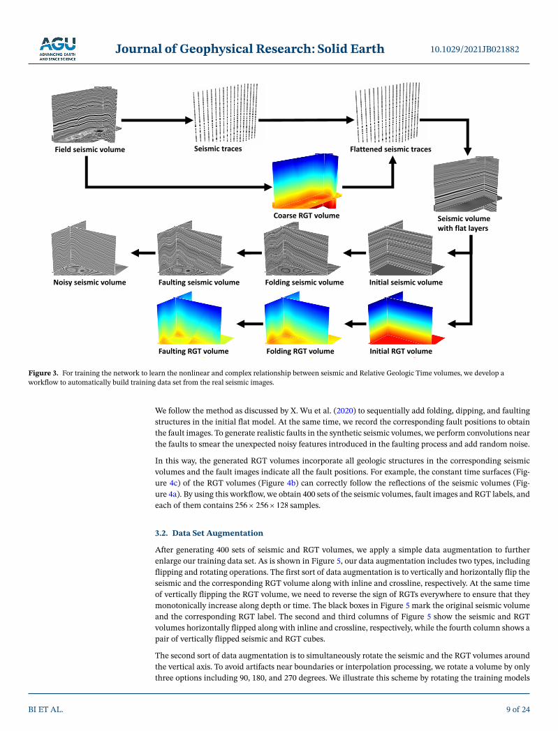
The RGT estimation is a supervised learning task that generally requires tremendous amounts of labeled data to obtain a network with great performance. However, it is hardly possible to fully label all the geologic structures within a field seismic survey. For appropriately training the network, we develop a workflow (Figure 3) to automatically build the sufficiently large training data set with various structural patterns. In this workflow, the first step is to create an initial seismic image with flat reflections and RGT volume with vertically monotonic values as the initial structural models. As is shown in Figure 3, to create a realistic initial seismic volume, we randomly select seismic traces from the real data and estimate a coarse RGT vol-ume by using the sloped-based method. Although this RGT volume might not accurately track the geologic structures, it provides structural information useful for flattening the extracted seismic traces. We horizon-tally spread the flattened traces to obtain the initial seismic image volume through interpolation. To further complicate the initial model, we use a Gaussian filter to perturb the seismic amplitude distributions, and an exponential operator to amplify the amplitude contrasts. Beginning from this initial model, we automatical-ly create a variety of synthetic samples with diverse and realistic structural features.


BI ET AL.

10.1029/2021JB021882

9 of 24

We follow the method as discussed by X. Wu et al. (2020) to sequentially add folding, dipping, and faulting structures in the initial flat model. At the same time, we record the corresponding fault positions to obtain the fault images. To generate realistic faults in the synthetic seismic volumes, we perform convolutions near the faults to smear the unexpected noisy features introduced in the faulting process and add random noise.

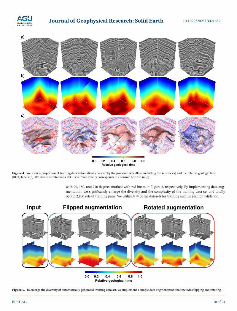
In this way, the generated RGT volumes incorporate all geologic structures in the corresponding seismic volumes and the fault images indicate all the fault positions. For example, the constant time surfaces (Fig-ure 4c) of the RGT volumes (Figure 4b) can correctly follow the reflections of the seismic volumes (Fig-ure 4a). By using this workflow, we obtain 400 sets of the seismic volumes, fault images and RGT labels, and each of them contains 256 256 128E samples.

3.2. Data Set Augmentation

After generating 400 sets of seismic and RGT volumes, we apply a simple data augmentation to further enlarge our training data set. As is shown in Figure 5, our data augmentation includes two types, including flipping and rotating operations. The first sort of data augmentation is to vertically and horizontally flip the seismic and the corresponding RGT volume along with inline and crossline, respectively. At the same time of vertically flipping the RGT volume, we need to reverse the sign of RGTs everywhere to ensure that they monotonically increase along depth or time. The black boxes in Figure 5 mark the original seismic volume and the corresponding RGT label. The second and third columns of Figure 5 show the seismic and RGT volumes horizontally flipped along with inline and crossline, respectively, while the fourth column shows a pair of vertically flipped seismic and RGT cubes.

The second sort of data augmentation is to simultaneously rotate the seismic and the RGT volumes around the vertical axis. To avoid artifacts near boundaries or interpolation processing, we rotate a volume by only three options including 90, 180, and 270 degrees. We illustrate this scheme by rotating the training models

Figure 3. For training the network to learn the nonlinear and complex relationship between seismic and Relative Geologic Time volumes, we develop a workflow to automatically build training data set from the real seismic images.


BI ET AL.

10.1029/2021JB021882

10 of 24

with 90, 180, and 270 degrees marked with red boxes in Figure 5, respectively. By implementing data aug-mentation, we significantly enlarge the diversity and the complexity of the training data set and totally obtain 2,800 sets of training pairs. We utilize 90%E of the datasets for training and the rest for validation.

Figure 4. We show a proportion of training data automatically created by the proposed workflow, including the seismic (a) and the relative geologic time (RGT) labels (b). We also illustrate that a RGT isosurface exactly corresponds to a seismic horizon in (c).

Figure 5. To enlarge the diversity of automatically generated training data set, we implement a simple data augmentation that includes flipping and rotating.


BI ET AL.

10.1029/2021JB021882

11 of 24

4. Training and ValidationWe train and validate our CNN model by using 2,500 and 300 3-D seismic volumes and the corresponding RGT labels, respectively. To avoid any uncertainties related to the seismic amplitude variations across dif-ferent surveys, we perform a normalization scheme for both input seismic images and the RGT labels, in which they are subtracted by the mean and then divided by the standard deviation to obtain the normalized volumes. When training the network, we formulate the normalized seismic and RGT volumes in batches and set the batch size to be 4, considering both the computation time and the hardware memory. An optimal learning strategy is to speed up the training by setting a suitable initial learning rate until the validation accuracy appears to plateau, and then slow down the parameter updates by decreasing the learning rate in a gradual manner. It can be achieved through learning rate schedules to automatically anneal the learning rate based on how many epochs through the data have been done and when the performance criterion has stopped improving. However, this typically adds additional hyper-parameters to control how quickly the learning rate decays. Based on the numerical experiments, we set the total iteration number to be 400, and the initial learning rate to be 0.0008 which reduces by a factor of 0.5 when the validation metric stagnates within 2 epochs (Figure 7c) to achieve an excellent tradeoff between the loss convergence and the com-putational efficiency. Although we cannot make sure this hyper-parameter combination is the best one, further hyper-parameter tuning is much time-consuming for a 3-D deep network but hardly obtain better improvements.

From Figure 7a, the loss curves for both training and validation gradually converge to less than 0.002 and 0.003 after 400 epochs when the optimization stops (Figure 7b), which indicates that the network has ac-curately captured the structural patterns in the seismic image volumes. It can be supported by the various quality metrics of RMSE, MAE, and MRPD shown in Figure 7c, which all decrease to the stable levels (0.027, 0.011, and 0.036). To demonstrate the performance of the trained network, we randomly select eight seismic images in the validation data set as inputs of the network to predict the RGT volumes. The vali-dation data set includes another 300 sets of samples, which are not included in the training data set. We show the seismic volumes, targets, and estimated RGT volumes in Figures 6a–6c, in which we find that the predictions appear to be highly similar to the RGT labels.

As is mentioned in the previous section, a surface of constant seismic instantaneous phase considered as a horizon surface can be represented by isosurface of the RGT volume. To further determine the ability of our method, we extract a set of horizon surfaces by tracking the hyper-surfaces along the isovalues of each predicted result. From Figure 6d, we find that these surfaces consistently follow the geologic structures even across faults, which indicates an excellent prediction performance. Moreover, we further analyze the network performance on the validation data set by computing the HEE metric that directly evaluates the quality of the extracted horizons. As is shown in Table 1, the horizons errors between the ground truth and predictions are all within 1 sample, which is considered to be not very significant in the seismic interpreta-tion. Therefore, we claim that the network has successfully learned to extract the general structural patterns from the seismic images due to its remarkable performance on both the training and validation datasets. In addition to the horizon interpolation, we can further detect the faults (Figure 6e) that are highlighted as sharp structural edges in the RGT volume, without computing the extra fault-related attribute images such as fault likelihood, strike, and dip.

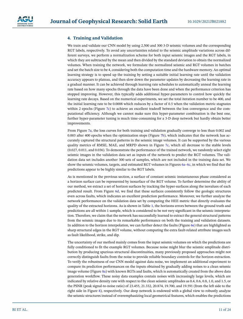
The uncertainty of our method mainly comes from the input seismic volumes on which the predictions are fully conditioned to fit the example RGT volumes. Because noise might blur the seismic amplitude distri-bution by producing spurious structural discontinuities, many previously proposed approaches might not correctly distinguish faults from the noise to provide reliable boundary controls for the horizon extraction. To verify the robustness of our CNN model against data noise, we implement an additional experiment to compare its prediction performances on the inputs obtained by gradually adding noises to a clean seismic image volume (Figure 8a) with known RGTs and faults, which is automatically created from the above data generation workflow. These noisy data examples contain noises with increasingly large levels, which are indicated by relative density rate with respect to the clean seismic amplitudes as 0.4, 0.6, 0.8, 1.0, and 1.5, or the PSNR (peak signal-to-noise ratio) of 23.455, 21.332, 20.874, 19.700, and 19.591 (from the left side to the right side in Figure 8), respectively. Our deep network is endowed with a global view to robustly analyze the seismic structures instead of overemphasizing local geometrical features, which enables the predictions


BI ET AL.

10.1029/2021JB021882

12 of 24

to be highly resilient to data noise. As is shown in Figures 8b–8f, the predicted RGT volumes show similar structural features in comparison to the ground truth marked by the black box, which can be supported by the great consistency between the detected faults and horizon surfaces extracted along RGT isovalues. However, although the network accurately captures the general variations of the seismic structures, it might not to correctly distinguish noisy structural discontinuities and detect the faults with relatively small dis-placements. When the noisy level becomes high enough to suppress the lateral reflection discontinuities, the fault-related features are highly complicated and not obvious in the seismic image volume. In this case, the faults might not be represented as apparently sharp edges in the predicted RGT volume, such that they are part and even completely missing in the following fault detection map. However, as is displayed in Figures 8e and 8f, deep learning still shows its promising robustness to produce an accurate RGT volume consistent with the seismic volume that is highly contaminated by noise.

5. Field Data ApplicationsIn addition to the synthetic examples, we test the network trained only with synthetic data on real seismic volumes from two field datasets to verify its general ability in analyzing seismic structural patterns. Differ-ent from the processing for training samples, the field seismic cubes are not augmented before fed to the network. To be consistent with the training data set, all of the input seismic volumes are subtracted by their means and divided by the standard deviations to obtain the normalized volumes. For a comparison purpose, we additionally compute the RGT volume by using a conventional (slope-based) method as the reference in these field data applications without any known geologic models.

Figure 6. We show the eight randomly selected seismic volumes and fault labels (a), labeled relative geologic time (RGT) volumes (b), predicted RGT volumes (c), and the seismic horizons (d) and fault positions (e) extracted from the predicted RGT volumes, respectively.


BI ET AL.

10.1029/2021JB021882

13 of 24

5.1. Case Study One

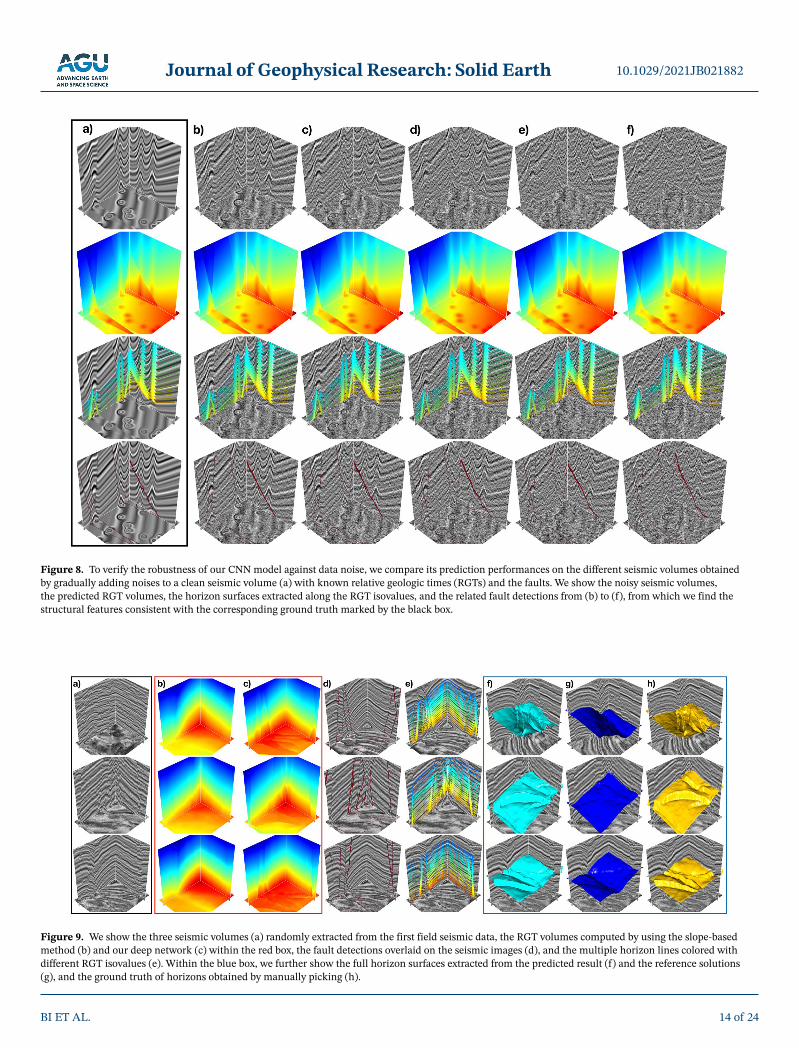
The first field seismic volume is a portion of the westCam data set, from which we randomly extract three seismic cubes (Figure 9a) with the same size of the training data set (128 256 256E ) and feed them into the trained network to predict the corresponding RGT volumes. In these seismic volumes, most of the re-flections appear to be flat, and the main difficulty is to distinguish closely spaced faults with large slips from noisy features. Because of the complex fault system and strong noise, calculating an accurate RGT volume remains a challenge in the existing methods.

Figure 9c displays the RGT volumes predicted from the trained network, and Figure 9e shows the surfac-es extracted along the constant RGT isovalues overlaid on the seismic volumes. By contrast to the RGT volumes estimated by using the slope-based method shown in Figure 9b (called reference solutions), the predicted results preserve more sharp structural features of the seismic image, and the RGT isosurfaces

Figure 7. (a) Training (red) and validation (cyan) loss curves; (b) During the training process, the learning rate is adaptively adjusted; (c) The recording histories of the quality metrics in validation. The dash and solid lines represent the curves with and without smoothing, respectively.

3-D network

Volume-based metrics Horizon-based metrics

Total GPU memory (MB)Trainable

parametersMAE RMSE MRPD SSIM HEE

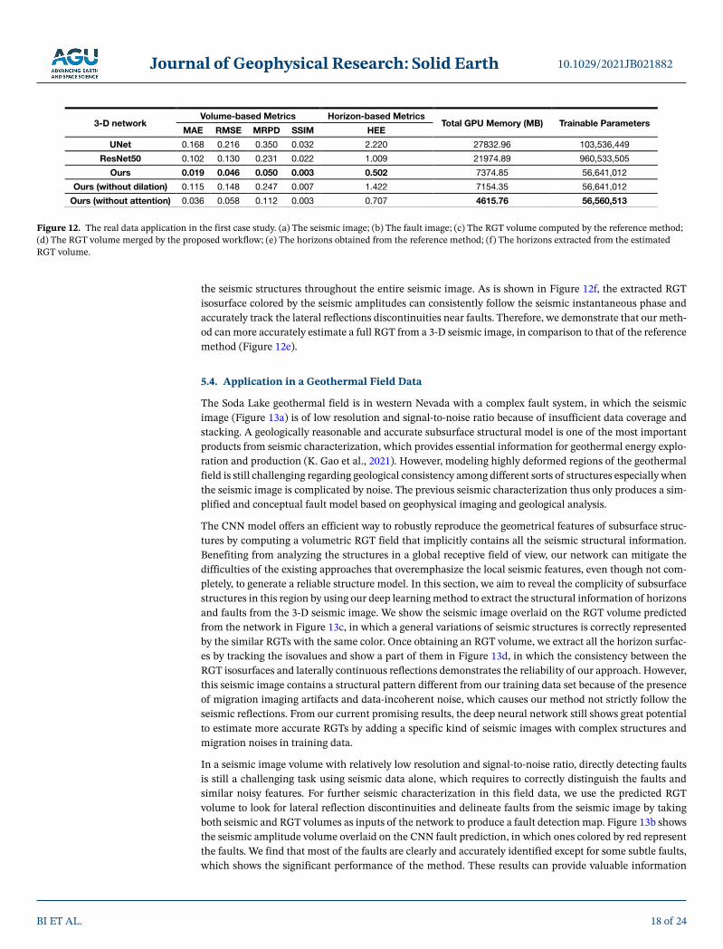
UNet 0.168 0.216 0.350 0.032 2.220 27,832.96 103,536,449

ResNet50 0.102 0.130 0.231 0.022 1.009 21,974.89 960,533,505

Ours 0.019 0.046 0.050 0.003 0.502 7374.85 56,641,012

Ours (without dilation) 0.115 0.148 0.247 0.007 1.422 7154.35 56,641,012

Ours (without attention) 0.036 0.058 0.112 0.003 0.707 4615.76 56,560,513

Note. The loss function used in each method is SSIM. For all the quality metrics, smaller value indicates better performance, and the best result is highlighted in bold.

Table 1 The Comparison of Different Relative Geologic Time Estimation Networks (UNet, ResNet50-Based Network (Geng et al., 2020), Our Network Without Attention Mechanism and Without Dilated Convolution in the Deepest Level)


BI ET AL.

10.1029/2021JB021882

14 of 24

Figure 8. To verify the robustness of our CNN model against data noise, we compare its prediction performances on the different seismic volumes obtained by gradually adding noises to a clean seismic volume (a) with known relative geologic times (RGTs) and the faults. We show the noisy seismic volumes, the predicted RGT volumes, the horizon surfaces extracted along the RGT isovalues, and the related fault detections from (b) to (f), from which we find the structural features consistent with the corresponding ground truth marked by the black box.

Figure 9. We show the three seismic volumes (a) randomly extracted from the first field seismic data, the RGT volumes computed by using the slope-based method (b) and our deep network (c) within the red box, the fault detections overlaid on the seismic images (d), and the multiple horizon lines colored with different RGT isovalues (e). Within the blue box, we further show the full horizon surfaces extracted from the predicted result (f) and the reference solutions (g), and the ground truth of horizons obtained by manually picking (h).


BI ET AL.

10.1029/2021JB021882

15 of 24

can consistently follow the laterally discontinuous reflections across faults. In addition, the fault-related features are implicitly embedded in the RGT volume and enhanced by apparent structural edges, even for those tiny and closely spaced faults, which contributes to an improved version of the fault interpretation. As is displayed in Figure 9d, the major faults with large slips are all masked by ones with red colors, which are consistent with the lateral reflection discontinuities along seismic horizons. These observations indicate that our method works well on this field data set, although the structural patterns and wavelet frequencies are different from the training seismic images.

To further verify the performance of the method, we extract a horizon surface from each of the predicted results and the reference solutions, and show them overlaid with the seismic volume in Figures 9f and 9g, respectively. In comparison to the reference solutions, we observe that the horizons extracted from the pre-dicted RGT volumes more consistently follow the seismic structures as they are obviously dislocated across faults. For evaluating the accuracy of each horizon, we manually pick a horizon line for every 5 sections of the seismic volume along inline and crossline, and then interpolate a horizon surface that crosses the full volume, which can be considered as the ground truth of the horizon surface (Figure 9h). As is shown in Figures 9f and 9h, even though the two sets of horizon surfaces are independently computed, they present highly similar geometrical features, which demonstrates the reliable generalization of our CNN model in this field data example.

5.2. Case Study Two

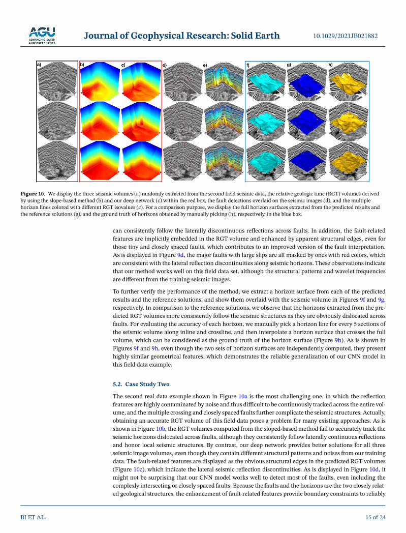
The second real data example shown in Figure 10a is the most challenging one, in which the reflection features are highly contaminated by noise and thus difficult to be continuously tracked across the entire vol-ume, and the multiple crossing and closely spaced faults further complicate the seismic structures. Actually, obtaining an accurate RGT volume of this field data poses a problem for many existing approaches. As is shown in Figure 10b, the RGT volumes computed from the sloped-based method fail to accurately track the seismic horizons dislocated across faults, although they consistently follow laterally continuous reflections and honor local seismic structures. By contrast, our deep network provides better solutions for all three seismic image volumes, even though they contain different structural patterns and noises from our training data. The fault-related features are displayed as the obvious structural edges in the predicted RGT volumes (Figure 10c), which indicate the lateral seismic reflection discontinuities. As is displayed in Figure 10d, it might not be surprising that our CNN model works well to detect most of the faults, even including the complexly intersecting or closely spaced faults. Because the faults and the horizons are the two closely relat-ed geological structures, the enhancement of fault-related features provide boundary constraints to reliably

Figure 10. We display the three seismic volumes (a) randomly extracted from the second field seismic data, the relative geologic time (RGT) volumes derived by using the slope-based method (b) and our deep network (c) within the red box, the fault detections overlaid on the seismic images (d), and the multiple horizon lines colored with different RGT isovalues (c). For a comparison purpose, we display the full horizon surfaces extracted from the predicted results and the reference solutions (g), and the ground truth of horizons obtained by manually picking (h), respectively, in the blue box.


BI ET AL.

10.1029/2021JB021882

16 of 24

estimate the horizon surfaces (Figure 10e). The consistency between the faults and horizons (Figures 10d and 10e) again validate the predicted RGT volumes are accurate and reliable.

To further verify the effectiveness of our deep network, we extract the horizon surfaces from the predicted results (Figure 10g) and the reference solutions (Figure 10h), then which are compared with the ground truth of horizons obtained by manually picking. Because all the structural information is implicitly em-bedded in the spatial distribution of RGTs, the extracted horizons can be used to evaluate the reliability of the predicted RGT volumes. From Figure 10g, we find that the horizon surfaces extracted from the refer-ence solutions fail to accurately the seismic structures especially across faults. As is shown in Figures 10f and 10h, although the two sets of horizon surfaces are obtained from different schemes, the horizon sur-faces extracted from the predicted results share geometrical features similar to the ground truth. These observations demonstrate excellent performance of our CNN model in this field data application, and again support our previous discussions.

For both two real data applications, we never ensure to construct a specific type of the training samples with structural patterns, wavelet length, and noise types and intensities that are similar to the real seismic volumes. However, the network trained by only using synthetic data still shows remarkable performance by accurately predicting the RGT volumes to indicate all the structural information, although the extracted horizons might not strictly match the ground truth of the manually picking ones. That means the trained network has successfully learned to analyze the general structural information in a global sense of view instead of simply remembering the local feature patterns induced in the given training examples.

5.3. RGT Merge Workflow

Although we fix the volume sizes of our training data, the method can be applied to a large-scale seismic volume by using the workflow to first divide the full seismic volume into multiple overlapped sub-volumes and then merge their corresponding predicted results into a full RGT volume. In this workflow, we first divide a large-scale seismic volume into the multiple sub-volumes with sizes identical to the training data, in which the two adjacent sub-volumes need to be partially overlapped with each other. Then we take these sub-volumes as the network inputs to predict the corresponding RGT sub-volumes, and then horizontally (along inline or crossline) and vertically concatenate them to produce the full RGT volume that covers the entire seismic amplitudes.

To merge the two vertically overlapped sub-volumes (Figure 11a), we estimate an RGT shift image by aver-aging the residual sum along the vertical axis in their overlapped regions. Then we use this shift image to correct the RGTs in every horizontal slice of both RGT sub-volumes, in which the one adds the half of RGT shifts and the other subtracts. By doing this, the two shifted RGT sub-volumes can be consistently concate-nated with each other along the vertical axis. When merging the two horizontally overlapped sub-volumes along inline or crossline (Figure 11b), the problem we mainly concern is to look for a mapping function that links the RGTs in their partially overlapped regions. For this reason, we build a simple regression model to robustly fit the relations of the two sets of RGTs by minimizing a linear least squares equation supplement-ed by the Tikhonov regularization, which can be formulated as follows,

2 22 2,LG Xw y w ‖ ‖ ‖ ‖ (9)

in which E is the smooth strength for reducing the variance of the estimates, and E w represents a set of re-gression coefficients of the mapping function, and the E y and E X denote the vector and matrix transformed from the RGTs in the overlapped regions, respectively. Once obtaining the mapping function, we can trans-form all the RGTs in one of the sub-volumes into a new volume that can be consistently merged with the other. By repeatedly concatenating every two partially overlapped sub-volumes, we can obtain a new RGT volume with an increasingly large scale until all the sub-volumes are integrated into a single volume with the same size as the whole large seismic image.

A real data example is used to demonstrate the effectiveness of this workflow, in which we show how to merge all of the predicted RGT sub-volumes in the first field data application to form a full volume. We first divide the entire seismic image into the partially overlapped sub-volumes with the same size as the


BI ET AL.

10.1029/2021JB021882

17 of 24

training data samples, and then use the trained network to estimate the corresponding RGT sub-volumes. The overlapped regions are selected away from the edges to reduce the boundary effects caused by the zero-padding steps in the convolutional layers of the network. To merge the two horizontally overlapped sub-volumes, we compute a mapping function to robustly approximate the relations of the RGTs in their overlapped regions by solving a linear least squares equation, and then transform one of the RGT sub-vol-umes into a new volume that can be consistently concatenated with the other. By repeatedly performing this produce, we can integrate all the horizontally overlapped RGT sub-volumes into a set of large sub-vol-umes with the horizontal scale sizes identical to the full seismic image. For every two horizontally merged sub-volumes that have the overlapped regions, we compute an RGT shift image and apply it to both sub-vol-umes and make sure that they can be consistently concatenated with each other. Ultimately, we obtain a complete RGT volume that covers the whole seismic amplitudes.

We first show the RGT volume computed from the seismic image (Figure 12a) by using the reference slope-based method in Figure 12c. By contrast, Figure 12d then displays the full RGT volume obtained by merging all the RGT sub-volumes predicted from our network, in which the RGTs are clearly dislocated near the faults and the dislocation amounts indicate the fault displacements. With such an RGT volume, we are able to accurately detect all the faults from the 3-D seismic image by using the deep network that takes the seismic and RGT volumes as inputs to produce a fault detection map (Figure 12b). By extracting the isosurfaces from the merged RGT volume, we can construct the horizon surfaces that consistently track

Figure 11. We propose a workflow to vertically (a) and horizontally (b) merge multiple RGT sub-volumes to construct a larger RGT volume that covers all seismic image samples.


BI ET AL.

10.1029/2021JB021882

18 of 24

the seismic structures throughout the entire seismic image. As is shown in Figure 12f, the extracted RGT isosurface colored by the seismic amplitudes can consistently follow the seismic instantaneous phase and accurately track the lateral reflections discontinuities near faults. Therefore, we demonstrate that our meth-od can more accurately estimate a full RGT from a 3-D seismic image, in comparison to that of the reference method (Figure 12e).

5.4. Application in a Geothermal Field Data

The Soda Lake geothermal field is in western Nevada with a complex fault system, in which the seismic image (Figure 13a) is of low resolution and signal-to-noise ratio because of insufficient data coverage and stacking. A geologically reasonable and accurate subsurface structural model is one of the most important products from seismic characterization, which provides essential information for geothermal energy explo-ration and production (K. Gao et al., 2021). However, modeling highly deformed regions of the geothermal field is still challenging regarding geological consistency among different sorts of structures especially when the seismic image is complicated by noise. The previous seismic characterization thus only produces a sim-plified and conceptual fault model based on geophysical imaging and geological analysis.

The CNN model offers an efficient way to robustly reproduce the geometrical features of subsurface struc-tures by computing a volumetric RGT field that implicitly contains all the seismic structural information. Benefiting from analyzing the structures in a global receptive field of view, our network can mitigate the difficulties of the existing approaches that overemphasize the local seismic features, even though not com-pletely, to generate a reliable structure model. In this section, we aim to reveal the complicity of subsurface structures in this region by using our deep learning method to extract the structural information of horizons and faults from the 3-D seismic image. We show the seismic image overlaid on the RGT volume predicted from the network in Figure 13c, in which a general variations of seismic structures is correctly represented by the similar RGTs with the same color. Once obtaining an RGT volume, we extract all the horizon surfac-es by tracking the isovalues and show a part of them in Figure 13d, in which the consistency between the RGT isosurfaces and laterally continuous reflections demonstrates the reliability of our approach. However, this seismic image contains a structural pattern different from our training data set because of the presence of migration imaging artifacts and data-incoherent noise, which causes our method not strictly follow the seismic reflections. From our current promising results, the deep neural network still shows great potential to estimate more accurate RGTs by adding a specific kind of seismic images with complex structures and migration noises in training data.

In a seismic image volume with relatively low resolution and signal-to-noise ratio, directly detecting faults is still a challenging task using seismic data alone, which requires to correctly distinguish the faults and similar noisy features. For further seismic characterization in this field data, we use the predicted RGT volume to look for lateral reflection discontinuities and delineate faults from the seismic image by taking both seismic and RGT volumes as inputs of the network to produce a fault detection map. Figure 13b shows the seismic amplitude volume overlaid on the CNN fault prediction, in which ones colored by red represent the faults. We find that most of the faults are clearly and accurately identified except for some subtle faults, which shows the significant performance of the method. These results can provide valuable information

Figure 12. The real data application in the first case study. (a) The seismic image; (b) The fault image; (c) The RGT volume computed by the reference method; (d) The RGT volume merged by the proposed workflow; (e) The horizons obtained from the reference method; (f) The horizons extracted from the estimated RGT volume.


BI ET AL.

10.1029/2021JB021882

19 of 24

for optimizing well placement and geothermal energy production at the Soda Lake geothermal field, which also demonstrates the prospect of applying our approach to the geothermal field studies.

6. DiscussionIn this section, we discuss the current advantages and limitations of our deep RGT estimation network and the potential improvements what we will focus on in future research.

6.1. Improvements

Although the depth of representation is of crucial importance for many image processing tasks (K. He et al., 2016; Lim et al., 2017), simply stacking convolutional learning units to construct deeper networks can hardly obtain better improvements. Whether deeper networks can further contribute to seismic structural analysis and how to construct very deep trainable networks remains to be explored. In comparison to the 3-D counterpart of the ResNet50-based network (Geng et al., 2020) and UNet, the proposed network not only shows better performance by providing the smaller values of the quality metrics on the validating examples, but also use a much simpler architecture with fewer trainable parameters. This simplification is mainly associated with the significant reduction of the feature channels throughout the network, which contributes to an acceptable computational cost for a 3-D seismic image processing task. To guarantee the

Figure 13. Application in a geothermal field data. (a) The seismic image volume acquired in the SodaLake geothermal field; (b) The fault detection map overlaid on the seismic image volume; (c) The seismic image volume overlaid on the predicted RGT volume; (d) The multiple horizon surfaces extracted from the predicted RGT volume.


BI ET AL.

10.1029/2021JB021882

20 of 24

representational ability of this simplified network, we explicitly model the interdependencies across different channels and subsets of the inter-mediate feature maps through attention mechanism, which makes the network adaptively enhance informative features while suppressing irrel-evant ones. Although some feature maps are deleted from the CNN mod-el architecture, our method still achieves accurate RGT predictions and reliable generalization performance. Table 1 shows a quantitative com-parison between our network with and without attention mechanism, from which we find that the latter shows better performance because of the smaller values of the quality metrics.

In addition, we adopt dilated convolutions to expand the receptive field without additional parameter update and spatial resolution loss, allowing the decoder branch receives rich structural information to make predic-

tions. For example, the ResNet50-based network and UNet downsample the input seismic image volume by a factor of 32 and 16 in the encoder branch, whereas the proposed network downsamples it by a factor of 8. That means, when the input seismic volume contains 128 128 128E samples, the minimum sizes of encoded feature maps in the reference methods are 4 4 4E , and 8 8 8E , respectively. However, the spa-tial information of seismic structures might not be properly represented in those extremely small-size fea-ture maps, which finally hinders the representational power of the deep network. By contrast, the encoder branch in our network produces the minimum small-size feature maps with the sizes of up to 16 16 16E . Therefore, the decoder branch receives 64 times more values than the reference network (ResNet50-based network), which significantly improves its sensitivities for recognizing detail structural features that cover-ing a smaller number of seismic pixels. Benefiting from those detailed structural features, our network can more accurately estimate the RGTs from the seismic amplitude distribution pattern. The same conclusion can be drawn from an additional ablation study, in which we compare the performances of our CNN models with standard and dilated convolutions in the deepest scale level of the encoder branch. In this experiment, the network with the standard convolutions expands the receptive field by down-sampling and thus pro-duces the smaller feature maps fed into the decoder branch by contrast to the dilated convolutions. As is shown in Table 2, we find that our network supplemented by dilated convolutions exhibits better prediction performance because of the smaller values for all the quality metrics.

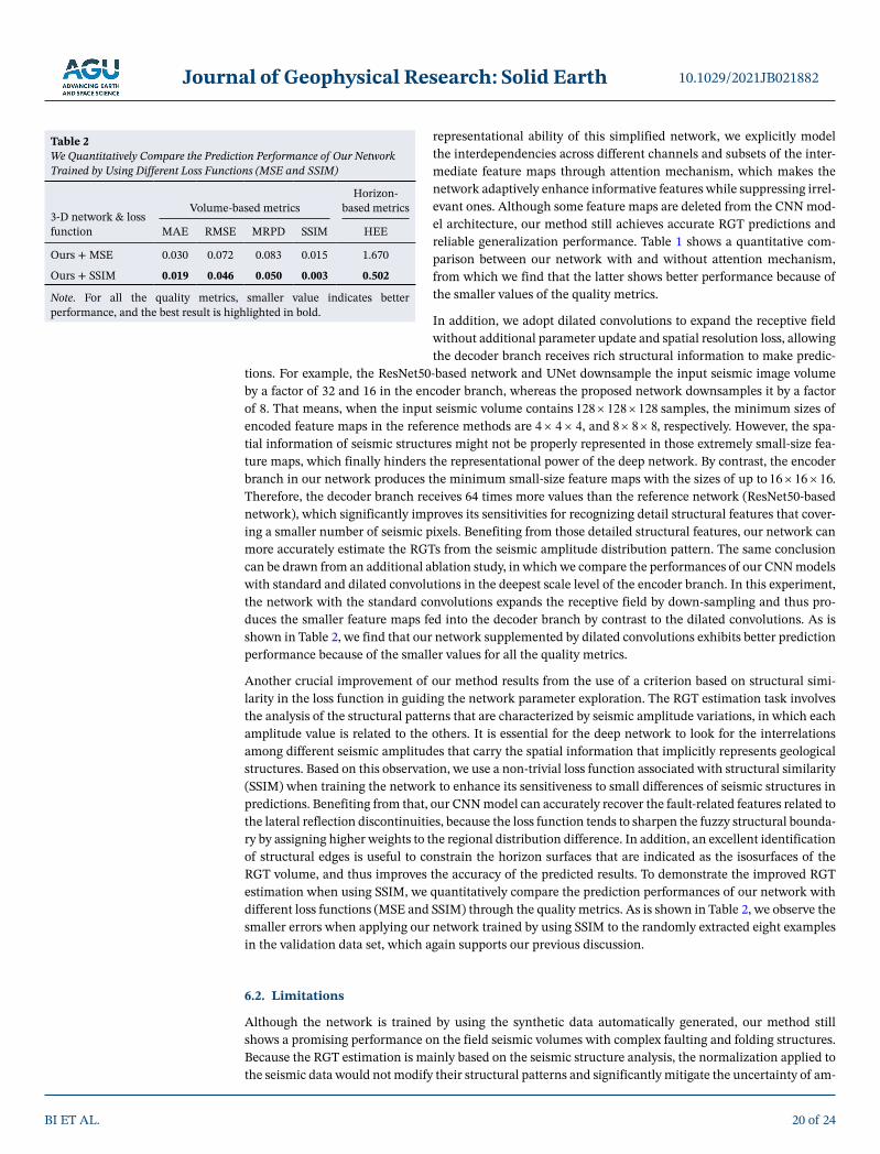
Another crucial improvement of our method results from the use of a criterion based on structural simi-larity in the loss function in guiding the network parameter exploration. The RGT estimation task involves the analysis of the structural patterns that are characterized by seismic amplitude variations, in which each amplitude value is related to the others. It is essential for the deep network to look for the interrelations among different seismic amplitudes that carry the spatial information that implicitly represents geological structures. Based on this observation, we use a non-trivial loss function associated with structural similarity (SSIM) when training the network to enhance its sensitiveness to small differences of seismic structures in predictions. Benefiting from that, our CNN model can accurately recover the fault-related features related to the lateral reflection discontinuities, because the loss function tends to sharpen the fuzzy structural bounda-ry by assigning higher weights to the regional distribution difference. In addition, an excellent identification of structural edges is useful to constrain the horizon surfaces that are indicated as the isosurfaces of the RGT volume, and thus improves the accuracy of the predicted results. To demonstrate the improved RGT estimation when using SSIM, we quantitatively compare the prediction performances of our network with different loss functions (MSE and SSIM) through the quality metrics. As is shown in Table 2, we observe the smaller errors when applying our network trained by using SSIM to the randomly extracted eight examples in the validation data set, which again supports our previous discussion.

6.2. Limitations

Although the network is trained by using the synthetic data automatically generated, our method still shows a promising performance on the field seismic volumes with complex faulting and folding structures. Because the RGT estimation is mainly based on the seismic structure analysis, the normalization applied to the seismic data would not modify their structural patterns and significantly mitigate the uncertainty of am-

3-D network & loss function

Volume-based metricsHorizon-

based metrics

MAE RMSE MRPD SSIM HEE

Ours + MSE 0.030 0.072 0.083 0.015 1.670

Ours + SSIM 0.019 0.046 0.050 0.003 0.502

Note. For all the quality metrics, smaller value indicates better performance, and the best result is highlighted in bold.

Table 2 We Quantitatively Compare the Prediction Performance of Our Network Trained by Using Different Loss Functions (MSE and SSIM)


BI ET AL.

10.1029/2021JB021882

21 of 24

plitude variations across different surveys, which contributes to a reliable generalization. It is an important reason why our network, trained only by the synthetic data, could be successfully applied to the field data volumes recorded from totally different surveys with varying structural patterns. However, our network working well to identify faulting and folding structures might fail to deal with other geologic structures not included in the training data, such as salt geobodies, unconformities, and igneous intrusions. Our trained model also might not work well for the cases with low dip-angle thrust faults because we still did not consider this type of faults when building the current training data set. To improve the generalization of our network, it is necessary to further complicate our data generation workflow by adding more various structural patterns. In addition to the diversity of structures, the challenge also exists in how to obtain more realistic seismic volumes with specific geometrical features caused by spatially varying wavelet frequencies or migration imaging artifacts. Although these features are unrelated to structures and excluded from the RGT labels, they typically exert a large impact on the structural pattern by smearing amplitude distribu-tion and producing spurious seismic structures. Thus, the currently trained network might not accurately compute RGTs in this case, which causes the necessity of using additional preprocessing steps to mitigate their influence and highlight the structure-related features. That means the CNN model might show excel-lent performance on the seismic image volume with consistent geometrical features to the training data. However, from our current promising results in both validation and field data applications, the CNN still shows great potential to compute a reliable RGT volume that robustly conforms with the seismic structures. Considering our training data set is still relatively small to train a 3-D deep network, further works will focus on simulating more realistic seismic image volumes with more various geological structures in our data generation workflow. In addition, we can even add real seismic images with interpreted RGT labels in the training data set to guarantee the prediction performance and reliable generalization of our approach in the field data application.

In many problems that involve the analysis of local structural features from the seismic image volume (such as fault and salt body detection), the input data size of the network in the field application might be different from the training data. For the RGT estimation task, the seismic amplitude distributions carry essential spa-tial information about geological structures, which typically requires a global view to reveal their geometri-cal patterns. Such a global view can be obtained from a large receptive field of the deep CNN, allowing every predicted RGT to be conditioned on the information collected from the entire seismic volume. The receptive field size can be expanded by stacking more convolutional learning units to form deeper CNN, such that a deeper network is able to extract the structural features on a larger scale. However, training a deeper network well is often more difficult and time-consuming because of heavier parameter exploration and more expensive computational costs. Thus, we require the size of the input seismic volume to be smaller than the receptive field of the network to achieve great representational power and reliable generalization through global structural analysis. For this reason, we fix the volume sizes of the input seismic images as 128 256 256E in both the training and testing steps of our CNN model. To mitigate the limitation of the fixed input data size, we propose a workflow to first divide the full seismic volume and estimate sub-vol-umes of RGT, and then merge them into a full RGT volume without boundary artifacts. Thus, although the input seismic volumes of the network need to be the same sizes, our method still can be successfully applied to a large-scale seismic image volume larger than the training data.

7. ConclusionWe propose a volume-to-volume deep network to accurately compute an RGT volume from the seismic image volume without any manual picking constraints, which is further used to simultaneously interpret horizons and faults. This network is simplified from the originally more complicated UNet and supplement-ed by multi-scale residual learning and attention mechanisms to achieve acceptable computational costs but still preserve the high prediction accuracy for RGT estimation. The RGT estimation is mainly based on the analysis of the structural features characterized by seismic amplitude distribution pattern, in which each amplitude value is related to the others. Based on this observation, we use a non-trivial criterion based on structural similarity as the loss function in optimizing the network parameters. We train the network by using synthetic data, which are all automatically generated by sequentially adding folding and faulting structures to an initial flat seismic image and RGT volume. Our CNN model not only shows promising


BI ET AL.

10.1029/2021JB021882

22 of 24

prediction performance on the synthetic data not included in training but also works well in the multiple field seismic volumes that are recorded at totally different surveys to reliably capture complex structural features such as crossing faults and complicatedly folded horizons. The resulting RGT volumes contain all the structural information in the seismic image volume, from which we are able to extract all the horizon surfaces by simply tracking along the constant RGT isovalues. In addition, we also show how to accurately detect faults by training the same network that takes the seismic and RGT volumes as inputs to produce a fault detection map, because the fault-related features are highlighted by sharp structural edges in the RGT volume. The applications in the three field data examples demonstrate the prediction performance and reliable generalization ability of the trained CNN model. These results can provide valuable information by revealing complex subsurface structures, which is of importance to many human activities ranging from natural source exploration to geothermal energy production.

However, trained by the current datasets, the network working well on field data volumes with complicated faulting and folding structures might not correctly deal with other geological structures not included in the training data such as unconformities, salt geobodies, and igneous intrusions. Our trained model also might not work well for the cases with low dip-angle thrust faults because we still did not consider this type of faults when building the current training data set. To improve the generalization ability of our network, we need to further complicate our data generation workflow by increasing the diversity of geological structures to obtain more realistic seismic images and the corresponding RGT volumes, which is actually what we are planning to do in future research. To mitigate the limitation of fixed input data size, we propose a workflow to first divide the full seismic volume and estimate sub-volumes of RGT, and then merge them into a full RGT volume without boundary artifacts. Although the input seismic volumes of the network require to be the same shapes, our method still can be successfully applied to a large-scale seismic image volume larger than the training data.

Data Availability StatementThe 400 pairs of synthetic seismic volumes and the RGT labels, used for training and validating our net-work, are uploaded to Zenodo and are freely available through the DOI link https://doi.org/10.5281/zeno-do.4536561. The source code associated with this research are also available and can be accessed via the Zenodo URL: https://doi.org/10.5281/zenodo.5044922.

ReferencesAl-Dossary, S., & Marfurt, K. J. (2006). 3D volumetric multispectral estimates of reflector curvature and rotation. Geophysics, 71(5), P41–

P51. https://doi.org/10.1190/1.2242449Alliez, P., Cohen-Steiner, D., Tong, Y., & Desbrun, M. (2007). Voronoi-based variational reconstruction of unoriented point sets. Symposium

on Geometry Processing (Vol. 7, pp. 39–48).Badrinarayanan, V., Kendall, A., & Cipolla, R. (2017). Segnet: A deep convolutional encoder-decoder architecture for image segmentation.

IEEE Transactions on Pattern Analysis and Machine Intelligence, 39(12), 2481–2495. https://doi.org/10.1109/tpami.2016.2644615Bakker, P. (2002). Image structure analysis for seismic interpretation. (Unpublished doctoral dissertation). Delft University of Technology.Chen, L.-C., Papandreou, G., Kokkinos, I., Murphy, K., & Yuille, A. L. (2014). Semantic image segmentation with deep convolutional nets and

fully connected CRFs. arXiv preprint arXiv:1412.7062.Chen, L.-C., Papandreou, G., Kokkinos, I., Murphy, K., & Yuille, A. L. (2017). Deeplab: Semantic image segmentation with deep convo-

lutional nets, atrous convolution, and fully connected CRFs. IEEE Transactions on Pattern Analysis and Machine Intelligence, 40(4), 834–848.

Ciregan, D., Meier, U., & Schmidhuber, J. (2012). Multi-column deep neural networks for image classification. In 2012 IEEE conference on computer vision and pattern recognition (pp. 3642–3649).

Di, H., & Gao, D. (2016). Efficient volumetric extraction of most positive/negative curvature and flexure for fracture characterization from 3D seismic data. Geophysical Prospecting, 64(6), 1454–1468. https://doi.org/10.1111/1365-2478.12350

Di, H., Li, Z., Maniar, H., & Abubakar, A. (2020). Seismic stratigraphy interpretation by deep convolutional neural networks: A semisuper-vised workflow. Geophysics, 85(4), WA77–WA86. https://doi.org/10.1190/geo2019-0433.1

Duffy, O. B., Bell, R. E., Jackson, C. A.-L., Gawthorpe, R. L., & Whipp, P. S. (2015). Fault growth and interactions in a multiphase rift fault network: Horda platform, Norwegian North Sea. Journal of Structural Geology, 80, 99–119. https://doi.org/10.1016/j.jsg.2015.08.015

Figueiredo, A., Silva, F. B., Silva, P., de O. Martins, L., Milidiú, R. L., & Gattass, M. (2015). A clustering-based approach to map 3D seismic horizons. In 14th International congress of the Brazilian geophysical society & EXPOGEF, Rio de Janeiro, Brazil, 3–6 august 2015 (pp. 1166–1170). https://doi.org/10.1190/sbgf2015-233

Fomel, S. (2002). Applications of plane-wave destruction filters. Geophysics, 67(6), 1946–1960. https://doi.org/10.1190/1.1527095Fomel, S. (2010). Predictive painting of 3D seismic volumes. Geophysics, 75(4), A25–A30. https://doi.org/10.1190/1.3453847Gao, H., Wu, X., & Liu, G. (2020). Channel simulation and deep learning for channel interpretation in 3D seismic images. In Seg technical

program expanded abstracts 2020 (pp. 1449–1453). Society of Exploration Geophysicists. https://doi.org/10.1190/segam2020-3426477.1

AcknowledgmentsThis research was supported by the National Science Foundation of China under grant no. 41974121.

https://doi.org/10.5281/zenodo.4536561



https://doi.org/10.1190/1.2242449

https://doi.org/10.1109/tpami.2016.2644615

https://doi.org/10.1111/1365-2478.12350

https://doi.org/10.1190/geo2019-0433.1

https://doi.org/10.1016/j.jsg.2015.08.015

https://doi.org/10.1190/sbgf2015-233

https://doi.org/10.1190/1.1527095

https://doi.org/10.1190/1.3453847

https://doi.org/10.1190/segam2020-3426477.1


BI ET AL.

10.1029/2021JB021882

23 of 24

Gao, K., Huang, L., & Cladouhos, T. (2021). Three-dimensional seismic characterization and imaging of the soda lake geothermal field. Geothermics, 90, 101996. https://doi.org/10.1016/j.geothermics.2020.101996

Geng, Z., Wu, X., Shi, Y., & Fomel, S. (2020). Deep learning for relative geologic time and seismic horizons. Geophysics, 85(4), 1–47. https://doi.org/10.1190/geo2019-0252.1

Gersztenkorn, A., & Marfurt, K. J. (1999). Eigenstructure-based coherence computations as an aid to 3-D structural and stratigraphic mapping. Geophysics, 64(5), 1468–1479. https://doi.org/10.1190/1.1444651

Goodfellow, I., Bengio, Y., & Courville, A. (2016). Deep learning. MIT press.Grose, L., Laurent, G., Aillères, L., Armit, R., Jessell, M., & Caumon, G. (2017). Structural data constraints for implicit modeling of folds.

Journal of Structural Geology, 104, 80–92. https://doi.org/10.1016/j.jsg.2017.09.013Hale, D. (2009). Structure-oriented smoothing and semblance. CWP Report 635.Hale, D. (2012). Fault surfaces and fault throws from 3D seismic images. In Seg technical program expanded abstracts 2012 (pp. 1–6). Soci-

ety of Exploration Geophysicists. https://doi.org/10.1190/segam2012-0734.1Hale, D. (2013). Methods to compute fault images, extract fault surfaces, and estimate fault throws from 3D seismic images. Geophysics,

78(2), O33–O43. https://doi.org/10.1190/geo2012-0331.1He, K., Zhang, X., Ren, S., & Sun, J. (2016). Deep residual learning for image recognition. In Proceedings of the IEEE conference on computer

vision and pattern recognition (pp. 770–778). https://doi.org/10.1109/cvpr.2016.90He, Q., & Wang, Y. (2021). Reparameterized full-waveform inversion using deep neural networks. Geophysics, 86(1), V1–V13.Hongliu, Z., Xiaomin, Z., Rukai, Z., & Zhang, Q. (2012). Guidelines for seismic sedimentologic study in non-marine postrift basins. Petro-

leum Exploration and Development, 39(3), 295–304.Hu, J., Shen, L., Albanie, S., Sun, G., & Wu, E. (2020). Squeeze-and-excitation networks. IEEE Transactions on Pattern Analysis and Ma-

chine Intelligence, 42(8), 2011–2023.Irakarama, M., Laurent, G., Renaudeau, J., & Caumon, G. (2020). Finite difference implicit structural modeling of geological structures.

Mathematical Geosciences, 53, 785–808.Kappler, K., Kuzma, H. A., & Rector, J. W. (2005). A comparison of standard inversion, neural networks and support vector machines. In

Seg technical program expanded abstracts 2005 (pp. 1725–1727). Society of Exploration Geophysicists.Karimi, P., & Fomel, S. (2015). Stratigraphic coordinates: A coordinate system tailored to seismic interpretation. Geophysical Prospecting,

63(5), 1246–1255.Karimi, P., Fomel, S., Wood, L., & Dunlap, D. (2015). Predictive coherence. Interpretation, 3(4), SAE1–SAE7. https://doi.org/10.1190/

INT-2015-0030.1Krizhevsky, A., Sutskever, I., & Hinton, G. E. (2012). Imagenet classification with deep convolutional neural networks. In Advances in

neural information processing systems (pp. 1097–1105).Lacaze, S., Durot, B., Devilliers, A., & Pauget, F. (2017). Comprehensive seismic interpretation to enhance stratigraphy and faults. In 15th

International congress of the Brazilian geophysical society & EXPOGEF, Rio de Janeiro, Brazil, 31 July–3 August 2017 (p. 1429–1432).Laina, I., Rupprecht, C., Belagiannis, V., Tombari, F., & Navab, N. (2016). Deeper depth prediction with fully convolutional residual net-

works. In 2016 fourth international conference on 3D vision (pp. 239–248).Laurent, G., Ailleres, L., Grose, L., Caumon, G., Jessell, M., & Armit, R. (2016). Implicit modeling of folds and overprinting deformation.

Earth and Planetary Science Letters, 456, 26–38.LeCun, Y., Bengio, Y., & Hinton, G. (2015). Deep learning. Nature, 521(7553), 436–444.Li, F., & Lu, W. (2014). Coherence attribute at different spectral scales. Interpretation, 2(1). SA99–SA106.Liang, L., Hale, D., & Maučec, M. (2010). Estimating fault displacements in seismic images. In 80th annual international meeting, seg,

expanded abstracts (pp. 1357–1361).Lim, B., Son, S., Kim, H., Nah, S., & Mu Lee, K. (2017). Enhanced deep residual networks for single image super-resolution. In Proceedings

of the IEEE conference on computer vision and pattern recognition workshops (pp. 136–144).Lomask, J., Guitton, A., Fomel, S., Claerbout, J., & Valenciano, A. A. (2006). Flattening without picking. Geophysics, 71(4), 13–20.Lou, Y., Zhang, B., Lin, T., & Cao, D. (2020). Seismic horizon picking by integrating reflector dip and instantaneous phase attributes. Geo-

physics, 85(2), O37–O45.Luo, S., & Hale, D. (2013). Unfaulting and unfolding 3-D seismic images. Geophysics, 78(4), O45–O56.Marfurt, K. J., Kirlin, R. L., Farmer, S. L., & Bahorich, M. S. (1998). 3-D seismic attributes using a semblance-based coherency algorithm.

Geophysics, 63(4), 1150–1165.Marfurt, K. J., Sudhaker, V., Gersztenkorn, A., Crawford, K. D., & Nissen, S. E. (1999). Coherency calculations in the presence of structural

dip. Geophysics, 64(1), 104–111.Mitchum, R. M., Vail, P. R., & Thompson, S. (1977). Seismic stratigraphy and global changes of sea level: Part 2. The depositional sequence

as a basic Unit for stratigraphic analysis: Section 2. Application of seismic reflection configuration to stratigraphic interpretation. In M 26: Seismic Stratigraphy-Applications to Hydrocarbon Exploration (Vol. 26, pp. 53–62). AAPG Memoirs.

Monniron, M., Frambati, S., Quillón, S., Berthoumieu, Y., & Donias, M. (2016). Seismic horizon and pseudo-geological time cube extrac-tion based on a riemmanian geodesic search. In IEEE 12th image, video, and multidimensional signal processing workshop (IVMSP) (pp. 1–5). https://doi.org/10.1109/IVMSPW.2016.7528178

Nair, V., & Hinton, G. E. (2010). Rectified linear units improve restricted boltzmann machines. ICML.Oktay, O., Schlemper, J., Folgoc, L. L., Lee, M., Heinrich, M., Misawa, K., et al. (2018). Attention u-net: Learning where to look for the pan-

creas. arXiv preprint arXiv:1804.03999.Parks, D. (2010). Seismic image flattening as a linear inverse problem. (Unpublished master's thesis). Colorado School of Mines.Pedersen, S. I., Skov, T., Hetlelid, A., Fayemendy, P., Randen, T., & Sønneland, L. (2003). New paradigm of fault interpretation. In 73rd

annual international meeting, seg, expanded abstracts (pp. 350–353).Pham, N., Fomel, S., & Dunlap, D. (2019). Automatic channel detection using deep learning. Interpretation, 7(3), SE43–SE50.Posamentier, H., Davies, R., Cartwright, J., & Wood, L. (2007). Seismic geomorphology-An overview. In R. J. Davies, H.W. Posamentier, L.J.

Wood, J.A. Cartwright (eds.), Seismic geomorphology (Vol. 277, p. 1–14). Geological Society of London Special Publication.Prazuck, C., Durot, B., Savajol, V., & Lacaze, S. (2015). Interpretation of complex geo-bodies using a relative geological time model: Ex-

mouth sub-basin, Australia. In Seg technical program expanded abstracts 2015 (pp. 1643–1647). Society of Exploration Geophysicists.Reeve, M. T., Bell, R. E., Duffy, O. B., Jackson, C. A.-L., & Sansom, E. (2015). The growth of non-colinear normal fault systems; what can

we learn from 3D seismic reflection data. Journal of Structural Geology, 70, 141–155.Renaudeau, J., Malvesin, E., Maerten, F., & Caumon, G. (2019). Implicit structural modeling by minimization of the bending energy with

moving least squares functions. Mathematical Geosciences, 51(6), 693–724.

https://doi.org/10.1016/j.geothermics.2020.101996

https://doi.org/10.1190/geo2019-0252.1

https://doi.org/10.1190/geo2019-0252.1

https://doi.org/10.1190/1.1444651

https://doi.org/10.1016/j.jsg.2017.09.013

https://doi.org/10.1190/segam2012-0734.1

https://doi.org/10.1190/geo2012-0331.1

https://doi.org/10.1109/cvpr.2016.90

https://doi.org/10.1190/INT%2D2015-0030.1

https://doi.org/10.1190/INT%2D2015-0030.1

https://doi.org/10.1109/IVMSPW.2016.7528178


BI ET AL.

10.1029/2021JB021882

24 of 24

Roberts, A. (2001). Curvature attributes and their application to 3D interpreted horizons. First Break, 19(2), 85–100.Ronneberger, O., Fischer, P., & Brox, T. (2015). U-net: Convolutional networks for biomedical image segmentation. In International confer-

ence on medical image computing and computer-assisted intervention (pp. 234–241).Sen, S., Kainkaryam, S., Ong, C., & Sharma, A. (2020). Saltnet: A production-scale deep learning pipeline for automated salt model build-

ing. The Leading Edge, 39(3), 195–203.Shi, Y., Wu, X., & Fomel, S. (2019). SaltSeg: Automatic 3D salt segmentation using a deep convolutional neural network. Interpretation,

7(3), SE113–SE122.Simonyan, K., Vedaldi, A., & Zisserman, A. (2013). Deep inside convolutional networks: Visualising image classification models and saliency

maps. arXiv preprint arXiv:1312.6034.Stark, T. J. (2003). Unwrapping instantaneous phase to generate a relative geologic time volume. In Seg technical program expanded ab-

stracts 2003 (pp. 1707–1710). Society of Exploration Geophysicists.Stark, T. J. (2004). Relative geologic time (age) volumes—Relating every seismic sample to a geologically reasonable horizon. The Leading

Edge, 23(9), 928–932.Stark, T. J. (2005). Generating a seismic Wheeler volume. In 75th annual International meeting, Seg, expanded abstracts (pp. 782–785).

Society of Exploration Geophysicists.Stark, T. J. (2005). System for multi-dimensional data analysis. Google Patents. (US Patent 6,850,845).Stark, T. J. (2006). Visualization techniques for enhancing stratigraphic inferences from 3D seismic data volumes. First Break, 24(4).Ulyanov, D., Vedaldi, A., & Lempitsky, V. (2016). Instance normalization: The missing ingredient for fast stylization. arXiv preprint

arXiv:1607.08022.Van Bemmel, P. P., & Pepper, R. E. (2000). Seismic signal processing method and apparatus for generating a cube of variance values. Google

Patents. (US Patent 6,151,555).Wang, Z., Bovik, A. C., Sheikh, H. R., & Simoncelli, E. P. (2004). Image quality assessment: From error visibility to structural similarity.

IEEE Transactions on Image Processing, 13(4), 600–612.Wang, Z., Simoncelli, E. P., & Bovik, A. C. (2003). Multiscale structural similarity for image quality assessment.In The Thrity-Seventh

Asilomar Conference on Signals, Systems & Computers, 2003, (Vol. 2, p. 1398–1402).Wu, H., Zhang, B., Lin, T., Cao, D., & Lou, Y. (2019). Semiautomated seismic horizon interpretation using the encoder-decoder convolu-

tional neural network. Geophysics, 84(6), B403–B417.Wu, X., & Fomel, S. (2018a). Automatic fault interpretation with optimal surface voting. Geophysics, 83(5), O67–O82. https://doi.

org/10.1190/geo2018-0115.1Wu, X., & Fomel, S. (2018b). Least-squares horizons with local slopes and multigrid correlations. Geophysics, 83(4), IM29–IM40. https://

doi.org/10.1190/geo2017-0830.1Wu, X., Geng, Z., Shi, Y., Pham, N., Fomel, S., & Caumon, G. (2020). Building realistic structure models to train convolutional neural net-

works for seismic structural interpretation. Geophysics, 85(4), WA27–WA39.Wu, X., & Hale, D. (2015). Horizon volumes with interpreted constraints. Geophysics, 80(2), IM21–IM33.Wu, X., Liang, L., Shi, Y., & Fomel, S. (2019). Faultseg3-d: Using synthetic data sets to train an end-to-end convolutional neural network

for 3-d seismic fault segmentation. Geophysics, 84(3), IM35–IM45.Wu, X., Liang, L., Shi, Y., Geng, Z., & Fomel, S. (2019). Deep learning for local seismic image processing: Fault detection, structure-oriented

smoothing with edge-preserving, and slope estimation by using a single convolutional neural network. In Seg technical program expand-ed abstracts 2019 (pp. 2222–2226). Society of Exploration Geophysicists.

Wu, X., Luo, S., & Hale, D. (2016). Moving faults while unfaulting 3D seismic images. Geophysics, 81(2), IM25–IM33.Wu, X., & Zhong, G. (2012). Generating a relative geologic time volume by 3-D graph-cut phase unwrapping method with horizon and

unconformity constraints. Geophysics, 77(4), 21–34.Wu, Y., & McMechan, G. A. (2019). Parametric convolutional neural network-domain full-waveform inversion. Geophysics, 84(6),

R881–R896.Xie, S., & Tu, Z. (2015). Holistically-nested edge detection. In Proceedings of the IEEE international conference on computer vision (pp.

1395–1403).Xiong, W., Ji, X., Ma, Y., Wang, Y., AlBinHassan, N. M., Ali, M. N., & Luo, Y. (2018). Seismic fault detection with convolutional neural

network. Geophysics, 83(5), O97–O103.Yang, F., & Ma, J. (2019). Deep-learning inversion: A next-generation seismic velocity model building method. Geophysics, 84(4),

R583–R599.Yu, S., Ma, J., & Wang, W. (2019). Deep learning for denoising. Geophysics, 84(6), V333–V350.Zeng, K., & Wang, Z. (2012). 3D-SSIM for video quality assessment. In 2012 19th IEEE international conference on image processing (pp.

621–624).Zhang, Y., Li, K., Li, K., Wang, L., Zhong, B., & Fu, Y. (2018). Image super-resolution using very deep residual channel attention networks.

Proceedings of the European conference on computer vision (ECCV) (pp. 286–301).Zinck, G., Donias, M., Daniel, J., Guillon, S., & Lavialle, O. (2013). Fast seismic horizon reconstruction based on local dip transformation.

Journal of Applied Geophysics, 96, 11–18. https://doi.org/10.1016/j.jappgeo.2013.06.010

https://doi.org/10.1190/geo2018-0115.1

https://doi.org/10.1190/geo2018-0115.1

https://doi.org/10.1190/geo2017-0830.1

https://doi.org/10.1190/geo2017-0830.1

https://doi.org/10.1016/j.jappgeo.2013.06.010

Documents

Deep Relative Geologic Time: A Deep Learning Method for