Deep-Sea Research II 58 (2011) 628–644

Contents lists available at ScienceDirect

Deep-Sea Research II

0967-06

doi:10.1

� Corr

School

NSW 20

E-m

journal homepage: www.elsevier.com/locate/dsr2

Modelling coastal connectivity in a Western Boundary Current: Seasonal andinter-annual variability

Moninya Roughan a,b,�, Helen S. Macdonald a, Mark E. Baird a, Tim M. Glasby c

a Coastal and Regional Oceanography Laboratory, School of Mathematics and Statistics, University of New South Wales, Sydney, NSW 2052, Australiab Sydney Institute of Marine Science, Mosman, NSW, Australiac NSW Department of Industry and Investment, Port Stephens, NSW, Australia

a r t i c l e i n f o

Article history:

Received 15 June 2010

Accepted 15 June 2010Available online 1 July 2010

Keywords:

East Australian Current

Larval transport

Connectivity matrices

45/$ - see front matter Crown Copyright & 2

016/j.dsr2.2010.06.004

esponding author at: Coastal and Regiona

of Mathematics and Statistics, University of

52, Australia.

ail address: mroughan@unsw.edu.au (M. Rou

a b s t r a c t

Understanding the transport and distribution of marine larvae by ocean currents is one of the key goals

of population ecology. Here we investigate circulation in the East Australian Current (EAC) and its

impact on the transport of larvae and coastal connectivity. A series of Lagrangian particle trajectory

experiments are conducted in summer and winter from 1992–2006 which enables us to investigate

seasonal and inter-annual variability. We also estimate a mean connectivity state from the average of

each of the individual realisations. Connectivity patterns are related to the movement of five individual

larval species (two tropical, two temperate and one invasive species) and are found to be in qualitative

agreement with historical distribution patterns found along the coast of SE Australia.

We use a configuration of the Princeton Ocean Model to investigate physical processes in the ocean

along the coast of SE Australia where the circulation is dominated by the EAC, a vigorous western

boundary current. We assimilate hydrographic fields from a � 10-km global analysis into a � 3-km

resolution continental shelf model to create a high-resolution hindcast of ocean state for each summer

and winter from 1992–2006. Particles are released along the coast of SE Australia, and at various

isobaths across the shelf (25–1000 m) over timescales ranging from 10–90 days. Upstream of the EAC

separation point across-shelf release location dominates the particle trajectory length scales, whereas

seasonality dominates in the southern half of the domain, downstream of the separation point.

Lagrangian probability density functions show dispersion pathways vary with release latitude,

distance offshore and the timescale of dispersion. Northern (southern) release sites are typified by

maximum (minimum) dispersal pathways. Offshore release distance also plays a role having the

greatest impact at the mid-latitude release sites. Maximum alongshore dispersion occurs at the

mid-latitude release sites such as Sydney. Seasonal variability is also greatest at mid-latitudes,

associated with variations in the separation point of the EAC. Climatic variations such as El Nino and La

Nina are also shown to play a role in dictating the connectivity patterns. La Nina periods have a

tendency to increase summer time connectivity (particularly with offshore release sites) while El Nino

periods are shown to increase winter connectivity.

The EAC acts as a barrier to the onshore movement of particles offshore, which impacts on the

connectivity of offshore release sites. Consequentially particles released inshore of the EAC jet exhibit a

greater coastal connectivity than those released offshore of the EAC front. The separation point of the

EAC also dictates connectivity with more sites being connected (with lower concentration) downstream

of the separation point of the EAC. These results can provide a useful guide to the potential connectivity

of marine populations, or the spread of invasive pests (via ballast water or release of propagules from

established populations).

Crown Copyright & 2010 Published by Elsevier Ltd. All rights reserved.

1. Introduction

The pelagic dispersal of marine larvae links populations acrossa wide geographic range and reduces their chance of extinction

010 Published by Elsevier Ltd. All

l Oceanography Laboratory,

New South Wales, Sydney,

ghan).

(Johannes, 1978). The supply of larvae (both numbers and timingof arrival), that can be affected by oceanographic conditions andbehaviourally dependent connectivity patterns, can play a criticalrole in determining the distribution and abundance of manymarine species. Understanding and predicting the spatial dis-tribution of organisms is among one of the most important goalsin population ecology (Siegel et al., 2003).

The importance and scale of long-distance dispersal of larvaeby oceanic currents has been well documented (e.g., Booth et al.,

rights reserved.

M. Roughan et al. / Deep-Sea Research II 58 (2011) 628–644 629

2007), and in some cases the patterns of dispersal have beenmodelled (e.g., North et al., 2008; Fox et al., 2009). But in general,there is little detailed understanding of the connectivity of marinepopulations via oceanic currents (Largier, 2003). Such informationis, however, important for a variety of purposes includingdesigning the size and arrangement of marine protected areas(Botsford et al., 2003), managing commercial fish stocks and forunderstanding (and helping to manage) the spread of marinepests (Glasby and Lobb, 2008). The dispersal of marine pests hastypically been quantified in relation to more easily measuredvectors such as ships (hulls and ballast water), or aquacultureinfrastructure (Carlton, 1987; Ruiz et al., 1997). But the potentialfor pests to disperse via currents is enormous as propagules ofmany species can remain in the water column for periods ofweeks to months.

Previously estimates of dispersal have relied on eithersimplified advection diffusion models or passive particle modelsthat use mean currents to define the potential for spread (Largier,2003; Cowen et al., 2006). In recent times, progress has beenmade in understanding the connectivity of populations in simpleflow environments using idealised models (Aiken et al., 2007;Bode et al., 2006), and in region specific estimates of larvaldispersion (e.g., Xue et al., 2008; Condie and Andrewartha, 2008,inter alia). Increasingly high level circulation models are beingused to simulate the dispersion of passive and active particleswithin and among estuaries and in the coastal ocean (Mitaraiet al., 2009; Huret et al., 2007). With the improvement of physicalcirculation models it is now possible to run semi-realisticsimulations of the coastal environment at high spatial andtemporal resolution to aid an understanding of populationconnectivity (Gillanders et al., 2010).

In a complex western boundary current system the use of meancurrents gives a simplified approximation to the likely dispersionpatterns, and it does not allow for the spatial complexity of thecirculation (such as coastal separation, encroachment of the jet, orthe complex eddy field circulation). Nor do these methods typicallyaccount for seasonal and inter-annual variability, making it difficultto quantify the statistical (and biological) reliability of the model.Estimates of source and sink regions do not necessarily identify thepathway that larvae take between spawning and settlement.Furthermore transport pathways may affect population resilience,for example larvae caught in a rotating eddy for a month may bestarved of food, more prone to predation, or subject to less thanideal temperatures.

Here we address some of the shortcomings in oceanographicmodelling applied to connectivity questions in the East AustralianCurrent (EAC). We have used the output from a state of the artanalysis product and downscaled it into a regional configurationof the Princeton Ocean Model, (hereafter referred to as SEAPOMBaird et al., submitted for publication). We apply the resultantproduct to the question of connectivity in a western boundarycurrent.

The EAC is a typical western boundary current (WBC) in that itflows poleward from the tropics to more temperate waters. It ishighly energetic and transports both heat and biota in its swiftflowing core (up to 2 ms�1) along the coast of southeastern (SE)Australia. Typically at � 323S the current turns sharply south-eastward away from the Australian coast into the Tasman Sea andthe majority of the transport is directed eastward along theTasman Front with the remainder continuing southward along theAustralian coast. The EAC exhibits a strong seasonal cycle, with amaximum velocity at � 303S in summer (Ridgway and Godfrey,1997). Upon separation from the coast the EAC undergoes a strongretroflection that leads to vigorous meandering and eddygeneration due to non-linear dynamics. The poleward extensionof the EAC also has a maximum velocity during the Austral

summer. The EAC dominates shelf circulation and coastal impactsinclude current driven upwelling (Roughan and Middleton, 2002,2004; Roughan et al., 2003) that also has substantive effects onphytoplankton and zooplankton assemblages, particularly inregions where nutrient supply is common but intermittent (Bairdet al., 2006a, b). Downstream of the EAC separation point thecontinental shelf waters are dominated by the EAC eddy field.

One of the aims of this study is to investigate how dispersalpathways (particle trajectories) differ seasonally, inter-annually,with latitude and distance offshore. We have identified five speciesthat can be represented by these particle trajectory studies alongthe coast of SE Australia: damselfish (Pomacentridae), butterflyfish(Chaetodontidae), snapper (Pagrus auratus), blue mackeral (Scomber

australasicus) and European shore crab (Carcinus maenas). Each ofthese species spawn across different latitudinal ranges (tropical ortemperate), have been observed to ‘settle’ or survive along the coastof SE Australia, are broadcast spawners and vary in their pelagiclarval duration (PLD) from 15–60 days.

To date this is the first study of its kind to use a high leveloceanographic modelling technique in order to begin to quantifythe variability in connectivity and dispersion pathways in a WBC.Specifically the questions we wish to address are: (1) Can weidentify seasonal and inter-annual variability in particle trajec-tories and connectivity in a WBC? (2) Can we determine withsome degree of statistical reliability the connectivity of waters ina WBC and thereby indicate the potential connectivity or dispersalof marine populations?

2. Methods

2.1. Ocean circulation model description

Here we use a configuration of the Princeton Ocean Model (POM)to model physical processes in the ocean along the coast of SEAustralia. POM has a free surface, a curvilinear grid and verticalsigma coordinates. The velocity components; u, v and w correspondto velocities in the alongshore (x direction), offshore (y direction)and vertical (normal to the sigma surfaces) directions, respectively.The primitive equations are solved on an Arakawa-C staggered gridusing finite difference methods (Blumberg and Mellor, 1987). TheSmagorinsky (1963) scheme is utilised in calculating horizontaldiffusion and is applied with an inverse turbulent Prandtl number(TPRNI) of 1.0 and a horizontal diffusivity coefficient (HORCON) of0.1. Temperature and salinity are advected using three iterations ofthe Smolarkiewicz upstream advection scheme (Smolarkiewicz,1984). The Craig and Banner (1994) scheme for calculating thewave-driven flux of turbulent kinetic energy at the surface hasbeen implemented and a hydrostatic correction term for sigma-coordinate models has also been included (Chu and Fan, 2003).Coastal boundary conditions at the western boundary are: zeronormal velocity, free-slip tangential velocity and zero gradient forvertical velocity, temperature and salinity.

2.2. Model configuration

Over the last 10 years POM has been configured for the NSWcontinental shelf off the southeast coast of Australia (Marchesielloand Middleton, 2000; Oke and Middleton, 2001; Roughan et al.,2003; Baird et al., 2006a; Macdonald et al., 2009, inter alia) wherethe flow is dominated by the EAC. The model spans 1025 km ofthe NSW continental shelf between 281 and 37.51S. At 281S thegrid area spans 395 km east from 153.51 to 1571E and at 371S itspans 500 km east from 149.51 to 155.51E. The maximum depth ofthe domain is 2000 m. This configuration improves on previous NSW

Fig. 1. The regional bathymetry and model grid. The white lines show the outer

grid and every 10th gridline. A high resolution coastline is shown in black, with

light shading representing land cells in the model. The colour scale shows 2u

bathymetry (m). The 200 m isobath is shown in white the latitudes of the 24

particle release sites are indicated by the star. CR: Clarence River, (R2), CH: Coffs

Harbour (R4), ED: Eden (R24).

M. Roughan et al. / Deep-Sea Research II 58 (2011) 628–644630

shelf configurations as the minimum depth is reduced from 50 m to15 m and a better depiction of the coastline is used. This enablesbetter representation of shallow water and near shore processes.

The SEAPOM configuration has 130 and 325 grid cells in theeast–west and north–south directions, respectively (Fig. 1). Theresolution ranges from 1 to 6 km in the east direction and 1.5 to6 km in the north direction. There are 36 sigma levels withspacing ranging from 1.1% to 4.35% of the total depth. This givesmore resolution on the continental shelf and in the top andbottom layers, for example, in shallow water (15 m) the firstsigma level is less than 3 m thick. The model solves the external(barotropic) mode with a 1.7 s timestep and the internal(baroclinic) mode with a 60-s timestep.

2.3. Downscaling an eddy-resolving global ocean model for the

continental shelf

Here we use the Bluelink ocean data assimilation system(BODAS), an ensemble optimal interpolation system to assimilatedata into our high-resolution continental shelf model. BODAS, whichis one of the many Bluelink products (Oke et al., 2007) recreates theocean state once every seven days using temperature and salinitydata from a combination of satellite altimetry, Argo, XBT, TAO andother sources. This is then assimilated into a global ocean generalcirculation model with a 10-km spatial resolution around Australia,resulting in BRAN (BlueLink ReANalysis) (Oke et al., 2007;Brassington et al., 2006).

BRAN 2p1 is a daily hindcast of ocean state from 1992–2006.The present BRAN configuration, however, does not providesufficiently high resolution in the horizontal or the vertical toinvestigate shelf processes. Hence for applications such as the

transport of small particles, particularly those that may come intoshallow water within close proximity of the coast we downscalethe coarse resolution BODAS to initialise a higher-resolutioncontinental shelf model.

For the first time BODAS hydrographic fields have been used toforce the higher resolution SEAPOM configuration of the coastalocean off SE Australia (Baird et al., submitted for publication). Inthis project BODAS temperature and salinity fields are assimilatedinto the higher-resolution SEAPOM configuration, meaning that,what was previously an idealised numerical simulation of theEAC, is now a fairly realistic high-resolution hindcast of the oceanstate off the coast of SE Australia for any one day from 1992–2006.The reader is referred to Baird et al. (submitted for publication) forfull details of the circulation model, SEAPOM.

Along the eastern and southern boundaries we apply a volumeconstraining radiation boundary condition with relaxation thatpermits oblique waves to radiate outwards (Marchesiello et al.,2001) to elevation and the baroclinic horizontal velocity compo-nents. For the barotropic horizontal velocity components the Flathercondition is applied (Flather, 1976). The relaxation to BODAS occursonce every seven days over a 24-hour period, at every gridbox inthe horizontal and vertical. Sensitivity experiments showed that theoptimum relaxation strength (i.e. when the root mean square errorin sea-surface temperature (SST) is minimised over the continentalshelf) is when t¼ 1 d�1 (Baird et al., submitted for publication). Inaddition to BRAN forcing, SEAPOM has been forced with dailyaveraged wind fields (NCEP) and radiative fluxes for each period(Kalnay et al., 1996).

The advantages of our high-resolution SEAPOM model aremany. Most obviously is the resolution of the model both in space,and a higher resolution time step. We have a more advancedvertical mixing scheme, which is particularly important in shallowregions. The shelf topography is of a higher resolution (Fig. 1),which means that we are able to resolve alongshore locationsmore precisely. The bathymetry of the POM model is also moreaccurate; for example it was noted that in the BRAN2p1configuration, Lord Howe Island lies 600 m sub-surface. We haveincreased vertical resolution in the important continental shelfregion and sigma co-ordinates in the vertical which enables veryhigh resolution in shallow water (see Fig. 2, Baird et al., submittedfor publication). The resolution of SEAPOM should be able to betterdepict small scale processes, such as those on the continental shelf,or across tight fronts and eddies and enables investigations such asparticle dispersion scenarios.

2.4. Model initialisation

SEAPOM initialisation occurs in two stages. Stage one isdiagnostic where temperature and salinity are initially set toBODAS fields and held constant while allowing velocity to evolve.Stage two is prognostic where temperature and salinity areallowed to evolve and are relaxed to the BODAS data followingassimilation (once every seven days). Forcing such as solarradiation and surface winds are also introduced during this stage(Baird et al., submitted for publication). Stage two begins 14 days(two assimilation cycles) before the tracer experiments arecommenced.

2.5. Model validation and assessment

To be able to simulate connectivity patterns one must haveconfidence in the ocean circulation model. To this end, robustmodel validation and assessment was undertaken by Baird et al.(submitted for publication). Comparisons between observedvelocities (obtained with a shipboard ADCP) and temperature

33

32.8

32.6

32.4

32.2

32

Latit

ude

(S)

1.0 m s1

20 22 24 26 28

152 152.5 15333

32.8

32.6

32.4

32.2

32

1.0 m s1

Longitude (E)

Latit

ude

(S)

1.21

0.80.60.4

0.20

0.10.2

0.20.3

1

0.80.60.4

0.2

00.1

dept

h (m

)

152.3 152.4 152.5 152.6 152.7

0

50

100

1500

50

100

1500

50

100

150

0.6

Longitude (E)

°C

14

15

16

17

18

19

20

21

22

23

24

Fig. 2. Model data comparison. Surface velocities and temperature obtained from shipboard measurements (magenta arrows) during February 1999, compared with: (A)

SEAPOM; (B) BRAN; (C–E) show cross-sections of velocity and temperature along a line at 32.71S obtained from (C) observations, (D) SEAPOM and (E) BRAN. Dashed (solid)

lines indicate poleward (equatorward) alongshore flow.

M. Roughan et al. / Deep-Sea Research II 58 (2011) 628–644 631

(Roughan and Middleton, 2002, 2004), SEAPOM and BRAN (Fig. 2)during February 1999 show that SEAPOM performs better in thecomplex shelf region off Port Stephens. SEAPOM better capturesthe strength of the EAC jet offshore, the location of the zeroisotach as well as the northward counter current inshore of the jet(Fig. 2C, D, and E). BRAN does not capture the northward inshoreflow (Fig. 2A and B), it underestimates the strength of the jet, thelocation of the temperature front, and underestimates thestrength of the upwelling, indicated by warmer temperaturesthrough the bottom boundary layer. A further example of theimprovement in the temperature and velocity resolution of thedownscaled product (SEAPOM) is shown in Fig. 3 (Baird et al.,submitted for publication, their Fig. 12). While BRAN captures thegross features of the poleward flowing EAC (Fig. 3B) and itsseparation from the coast, SEAPOM (Fig. 3A) depicts a series ofcoastal eddies inshore of the separated WBC jet and a significantnorthward coastal flow. Such a flow field is commonly found inthe Port Stephens region (e.g., Fig. 2). This has major implicationsfor the transport of particles in a direction counter to that of theswift poleward flowing WBC.

2.6. Numerical experiments

In order to investigate seasonal and inter-annual variability 28different simulations were conducted spanning the Australsummer (DJF) and winter (JJA) starting from December (summer)of 1992 to August (winter) of 2006. Model day 0 is taken to be atthe end of the two stage initialisation, i.e. after 34 days, and isequivalent to a day close to the start of summer or winter (whichvaries each year as BODAS output is only every seven days).

2.7. Particle tracking

One of the applications of these high-resolution hindcasts is toinvestigate the trajectories and dispersion of particles underdifferent scenarios (e.g., year, season, release latitude, releaseisobath). Particles are moved in the model using a formulationbased on the advection–diffusion equation. We advect theparticles on-line using a 3-D particle tracking scheme availableas a POM add-on, which makes use of the model velocities(horizontal and vertical). At each time step we interpolate thevelocities linearly at the sub-gridscale level. Dispersion isincorporated into the particle tracking routine with the inclusionof a random walk component. The 2.5 level Mellor and Yamada(1982) turbulence closure scheme is used to calculate theinstantaneous turbulent kinetic energy (TKE) throughout themodel domain. The effects of sub-grid scale processes areapproximated by the turbulence diffusion terms, which are scaledas a random number normalised between 0 and 1 (Roughan et al.,2003; Xue et al., 2008).

A series of particle tracking simulations were conducted.Particles were released in the surface waters above variousisobaths of biological significance (25, 50, 100, 200 and 1000 m) at17�0.51 latitudinal intervals from 29–371S with seven extrarelease sites corresponding with the mouth of major estuariesalong the coast (Table 1, Fig. 1), giving a total of 120 particlerelease sites per simulation. Particles were released in the surfacesigma layer, i.e. at a depth of 0–3 m below the surface. Theoffshore locations were chosen to give flexibility in theinterpretation of the results. For example, wherever possible,vessels are required to discharge ballast water at least 200 nmfrom shore and in water at least 200 m deep to minimise chances

Fig. 3. Comparison of SST (colourbar, 1C) and velocity fields (black vectors, ms�1) from SEAPOM (l) and BRAN (r) (Baird et al., submitted for publication, Fig. 12).

Table 1The locations of the particle release sites from north to south.

Site Lat Lat band Estuary

R1 291 29 –

R2 29325u 29.5 Clarence River

R3 301 30 –

R4 30318u 30 Coffs Harbour

R5 30329u 30.5 Kalang River

R6 30339u 30.5 Nambucca River

R7 30352u 31 Southwest Rocks

R8 31325u 31.5 Port Macquarie

R9 31352u 32 Manning River

R10 32310u 32 Wallis Lake

R11 32341u 32.5 Port Stephens

R12 32355u 33 Port Hunter

R13 3335u 33 Lake Macquarie

R14 33334u 33.5 Hawksbury

R15 33349u 33.5 Sydney Harbour

R16 341 34 Botany Bay

R17 3434u 34 Port Hacking

R18 34327u 34.5 Port Kembla

R19 34354u 34.5 Shoalhaven River

R20 3535u 35 Jervis Bay

R21 35342u 35.5 Clyde River

R22 361 36 –

R23 36330u 36.5 –

R24 3733u 37 Eden

Major estuaries and nominal latitudinal bands are identified.

M. Roughan et al. / Deep-Sea Research II 58 (2011) 628–644632

of species arriving to ports or estuaries where they might settleand establish. Hence the releases above the 200- and 1000-misobaths could be representative of such events.

Ten particles were released from each release site on modeldays 0, 5, 10, 15 and 20, giving a total of 6000 particles foreach season (168,000 across 28 seasons). When a particlereaches a boundary (northern, eastern, southern or the westerncoastal boundary) it stops propagating. Settlement is consideredto have occurred when a particle comes within a third of a gridbox of the coast within each latitudinal band (i.e. in surfacewaters).

Large-scale flows will affect the displacement of the centre ofmass of patch, where as small scale variability will determine therelative dispersal of the larvae (Gabric and Parslow, 1994). The

EAC is an advection driven regime with along-shore velocities ofup to 2 ms�1, as such advection dominates over sub-grid scalediffusion. Additional particle tracking experiments were con-ducted to test the sensitivity of the results to the number ofparticles. Finally an additional high-density particle-trackingsimulation was undertaken for July–August 2004 to undertakemodel-data comparisons.

2.8. Biological parameters

In this study we do not include biological parametersexplicitly. However, we make approximations for pelagic larvalduration (PLD) by investigating particle trajectories on timescalesranging from 10–90 days, i.e. covering a wide range of planktonicdurations for marine propagules. We account for seasonalspawning preferences by comparing summer and winter simula-tions and we allow for preferences in depth by investigatingrelease sites over various isobaths across the shelf. We do notaccount for the role of larval behaviour (e.g., vertical andhorizontal swimming) in modifying trajectories, thus our discus-sion of the typical larval trajectories considers time frames priorto when the larvae are able to swim well. We acknowledge thatthe inclusion of diurnal vertical migration may alter the resultssignificantly (e.g., North et al., 2008; Roughan et al., 2005),however, this work is a first step towards understanding meanconnectivity along the coast of SE Australia. We only considercoastal settlement that by default accounts for habitat suitability;it also allows for an investigation into connectivity betweenestuaries. Applying these results to habitat suitability is thesubject of ongoing work.

In Section 6.1 we relate the simulated particle paths to fivespecific larval species that are found along the coast of SEAustralia as an example of how the results could be used. Theparticular species are chosen as they spawn across differentlatitudinal ranges (tropical or temperate), have been observed to‘settle’ or survive along the coast of SE Australia and because theyvary in their pelagic larval duration (PLD). We have chosen twotropical fish species, two temperate commercial fish species andone invasive marine pest. All species identified are broadcastspawners, hence the dispersion of particles is of particularrelevance for their survival. Furthermore, larvae are typically

M. Roughan et al. / Deep-Sea Research II 58 (2011) 628–644 633

confined to the mixed layer hence the approach used here ofsurface release sites is appropriate. The focus species are:

�

Figwh

(tem

sum

Damselfish (Pomacentridae): A tropical family which spawnsnorth of 281S and have been observed to settle as far as 371S,with a PLD of 15–30 days (Booth et al., 2007). Typically reefassociated fishes, but can occur down to depths of 40–50 m.

� Butterflyfish (Chaetodontidae): Also a tropical family which

spawns north of 251S, and has a PLD of 40–60 days (Hoeseet al., 2006) with settlement observed as far south as 371S(Booth et al., 2007). Typically associated with shallow (1–20 m)coral reefs.

� Snapper (Pagrus auratus): A temperate species of commercial

relevance which broadcast spawns and recruits in estuaries, witha PLD of 18–31 days (Kingsford and Atkinson, 1994). Breedingadults are associated with offshore rocky reefs extending from thenear shore out to the edge of the continental shelf.

� Blue Mackeral (Scomber australasicus): Neira and Keane (2008)

found greatest larval abundances 10 nm shoreward of the shelfbreak linked to bathymetric (100–125 m deep) and hydro-graphic factors (19–201C), typically in EAC or EAC ‘mix’ water,northwards of 34.61S. They spawn June–October (Neira andKeane, 2008) and PLD is approximately five weeks, however,they swim well after 3–4 weeks (I Suthers Pers. comm.).

� European shore crab (Carcinus maenas): Considered a marine pest

in Australia and many other countries. It is an estuarine specieswhose larvae can be transported across the shelf (observed up to

36 S

34 S

32 S

30 SSummer199410 day1 ms

Summer199430 day

Summe199460 day

36 S

34 S

32 S

30 SSummer200410 day

Summer200430 day

Summe200460 day

36 S

34 S

32 S

30 SWinter199310 day

Winter199330 day

Winter199360 day

150 E 154 E

36 S

34 S

32 S

30 SWinter200310 day

150 E 154 E

Winter200330 day

150 E

Winter200360 day

1 ms 1 ms

1 ms 1 ms 1 ms

1 ms1 ms1 ms

1 ms 1 ms 1 ms

. 4. Particle paths after 10, 30, 60 and 90 days (l-r) for the first tracer released at the 25

ite to blue as the latitude of particle seeding moves poleward, i.e. red (blue) for particle

perature) at the end each time period are overlayed in black arrows (shading). Each ro

mer 1994, winter 2003, summer 2004 (top–bottom).

40 km offshore) before being returned to estuaries where theysettle (Queiroga, 1996). It can have a larval duration around 30–40days in the Austral summer and 40–50 days in winter, dependingon water temperature (deRivera et al., 2007).

3. Results

3.1. Particle trajectories—seasonal and inter-annual variability

The main feature defining the movement of the particles along thecoast of SE Australia is the poleward flowing EAC, its separation fromthe coast and the mesoscale eddy field. During the study period thelocation of the separation point varies between 301 and 331S andhence the region where particles are advected offshore changesbetween years and seasons. Upstream of the EAC separation pointparticle trajectories are predominantly poleward (Fig. 4) particularlyat the mid-shelf and shelf break release sites (100-, 200- and 1000-misobaths, not shown). The near coastal release sites (25-m isobathshown in Fig. 4) do exhibit minimal northward transport. Between341 and 361S (i.e. downstream of the EAC separation) resultantparticle distributions are bi-modal. Particles tend to either remainadjacent to the coast or to be swept eastward to the open oceandepending on the proximity of the EAC to the coast and the positionof the EAC separation. In this way the EAC can act as a barrier to theonshore movement (and coastal connectivity) of particles releasedoffshore, aiding retention inshore of the jet, whereas particlescaptured within the EAC are driven offshore.

r Summer199490 day

r Summer200490 day

Winter199390 day

154 E 150 E 154 E

Winter200390 day

13 C

14 C

15 C

16 C

17 C

18 C

19 C

20 C

21 C

22 C

23 C

24 C

25 C1 ms

1 ms

1 ms

1 ms

m isobath. The colour of the particle path ranges from red through orange and

s seeded at northern (southern) latitudes. The instantaneous model velocities

w shows a different year and season as indicated in the panel, i.e. winter 1993,

a2 25m R2 W 10d b2 25m R2 W 30d c2 25m R2 W 60d d2 25m R2 W 90d%

of p

artic

les

a6 25m R15 W 10d b6 25m R15 W 30d c6 25m R15 W 60d d6 25m R15 W 90d

a10 25m R24 W 10d b10 25m R24 W 30d c10 25m R24 W 60d d10 25m R24 W 90d

a1 25m R2 S 10d b1 25m R2 S 30d c1 25m R2 S 60d d1 25m R2 S 90d

a5 25m R15 S 10d b5 25m R15 S 30d c5 25m R15 S 60d d5 25m R15 S 90d

a9 25m R24 S 10d b9 25m R24 S 30d c9 25m R24 S 60d d9 25m R24 S 90d

a4 1000m R2 W 10d b4 1000m R2 W 30d c4 1000m R2 W 60d d4 1000m R2 W 90d

a8 1000m R15 W 10d b8 1000m R15 W 30d c8 1000m R15 W 60d d8 1000m R15 W 90d

−500 0 500

a12 1000m R24 W 10d

−500 0 500Alongshore distance (km)

b12 1000m R24 W 30d

−500 0 500

c12 1000m R24 W 60d

−500 0 500

d12 1000m R24 W 90d

a3 1000m R2 S 10d b3 1000m R2 S 30d c3 1000m R2 S 60d d3 1000m R2 S 90d

a7 1000m R15 S 10d b7 1000m R15 S 30d c7 1000m R15 S 60d d7 1000m R15 S 90d

2575

2575

2575

2575

2575

2575

2575

2575

2575

2575

2575

2575 a11 1000m R24 S 10d b11 1000m R24 S 30d c11 1000m R24 S 60d d11 1000m R24 S 90d

Fig. 5. Larval trajectory lengths, i.e. the mean distance travelled by particles released at three sites (R2 (1-4), R15 (5-8), R24 (9-12)), inshore (25 m) and offshore (1000 m),

in summer and winter, for timescales of 10–90 days (L-R) where 0 km indicates the particle release site. The distances particles travelled are grouped into 100 km bins and

positive (negative) distance indicates equatorward (poleward) transport.

M. Roughan et al. / Deep-Sea Research II 58 (2011) 628–644634

Inter-annual variability in the particle paths is evident in Fig. 4where representative trajectories are shown for Summer 1994 and2004 and Winter 1993 and 2003 for each release at the 25 m isobathafter 10, 30, 60 and 90 days. The presence (Summer 1994, Winter1993) or absence (Summer 2004, Winter 2003) of the EAC eddy fielddictates the circulation from the separation point poleward.Recirculation and retention is a maximum when eddies are present,whereas poleward transport is a maximum when the EAC remainsattached to the coast to the southern end of the domain.

Particles tend to be advected more quickly during summer(Fig. 4) than winter, indicative of the strong seasonal cycle of theEAC. Furthermore northward movement is more pronouncedduring the winter simulations, e.g., Winter 1993 (discussed furtherbelow). The EAC circulation features clearly dominate the particletrajectories. The presence or absence of an EAC eddy also dictatescirculation and retention on the continental shelf region. When theeddy field is far offshore, coastal transport is northward down-stream of the EAC separation point. Northward coastal transportcan also be great when a cyclonic eddy encroaches on thecontinental shelf driving velocities of up to 1/ms northward,downstream of the separation point (e.g., off Sydney).

3.2. Trajectory timescales

Intuitively the length of the particle trajectories increases withtime from 10–90 days. In the first 10 days the majority of the

particles are constrained within close proximity of the coast, after30 days some particles have settled at the coast and some are stillwithin the coastal area but have not settled while others have leftthe coastal area. After 60 days nearly all particles have eithersettled or have left the coastal area and have been entrained intoeddies which break away from the EAC in the southern half of thedomain. By 90 days most of the particles have reached a boundarymeaning that they would have left the model domain if they hadnot already settled (Fig. 4).

3.3. Trajectory length scales

The mean trajectory length scales (i.e. the distance travelled bya particle) helps to identify the variability within the particletrajectories (Fig. 5). The distance travelled is considered to be thestraight line alongshore distance from the particle end point to itsorigin. Fig. 5 compares the mean distance travelled by particlesreleased at three sites (R2, R15, R24, where R2 is upstream of theEAC separation point and R15, R24 are downstream), inshore(25 m) and offshore (1000 m), in summer and winter, where 0 kmindicates the particle release site. The distances particles travelledare grouped into 100-km bins and positive (negative) distanceindicates equatorward (poleward) transport.

Obviously, the maximum distance travelled ð4500 kmÞ isaffected by the trajectory timescale (10, 30, 60 or 90 days).Inshore of the EAC jet, it can take 10–30 days for the particles to

M. Roughan et al. / Deep-Sea Research II 58 (2011) 628–644 635

leave the vicinity of the release point. It is here (Fig. 5, Column a)that length scale variability is greatest. By 60–90 (Fig. 5, Column cand d) days the importance of timescales gives way to coastalproximity and seasonality as most particles are eventuallyentrained into the EAC or advected out of the domain.

Proximity of the release site to the coast can also dictatedistance travelled. The inshore release sites (Fig. 5, Rows 1, 2, 5, 6,9, and 10) exhibit high variability particularly duringsummer, whereas the offshore release sites exhibit less variabilityparticularly during winter and especially upstream of theseparation point of the EAC (Fig. 5, Rows 1–4). Typically theoffshore release sites are in the core of the EAC (especiallyupstream of the separation point) and are advected polewardswiftly with less variability in the lengthscales. Seasonalitydominates the trajectory length scales at the southern releasesites (Fig. 5, Rows 9–12). This is consistent with the seasonality ofthe EAC (stronger and penetrating further southward in summerthan in winter).

Northward transport is a maximum in winter, particularly atthe downstream release sites (after 10 days, R2o100 km,R244400 km northward, after 90 days R244800 km northward),which is significant when investigating the dispersal pathways ofspecies that spawn in winter. At the southern release sites thenorthward transport is significantly greater than any of the morenorthern release sites. Poleward transport is least at the southernrelease sites; however, this is most likely an artefact of theproximity to the southern boundary of the model domain.Interestingly our results support the analysis of Coleman et al.(in preparation) who investigated the genetic variability inseaweed along the NSW coastline. They showed that geneticsimilarities between coastal kelp communities separated bydistance could be attributed to the less uniform nature of the

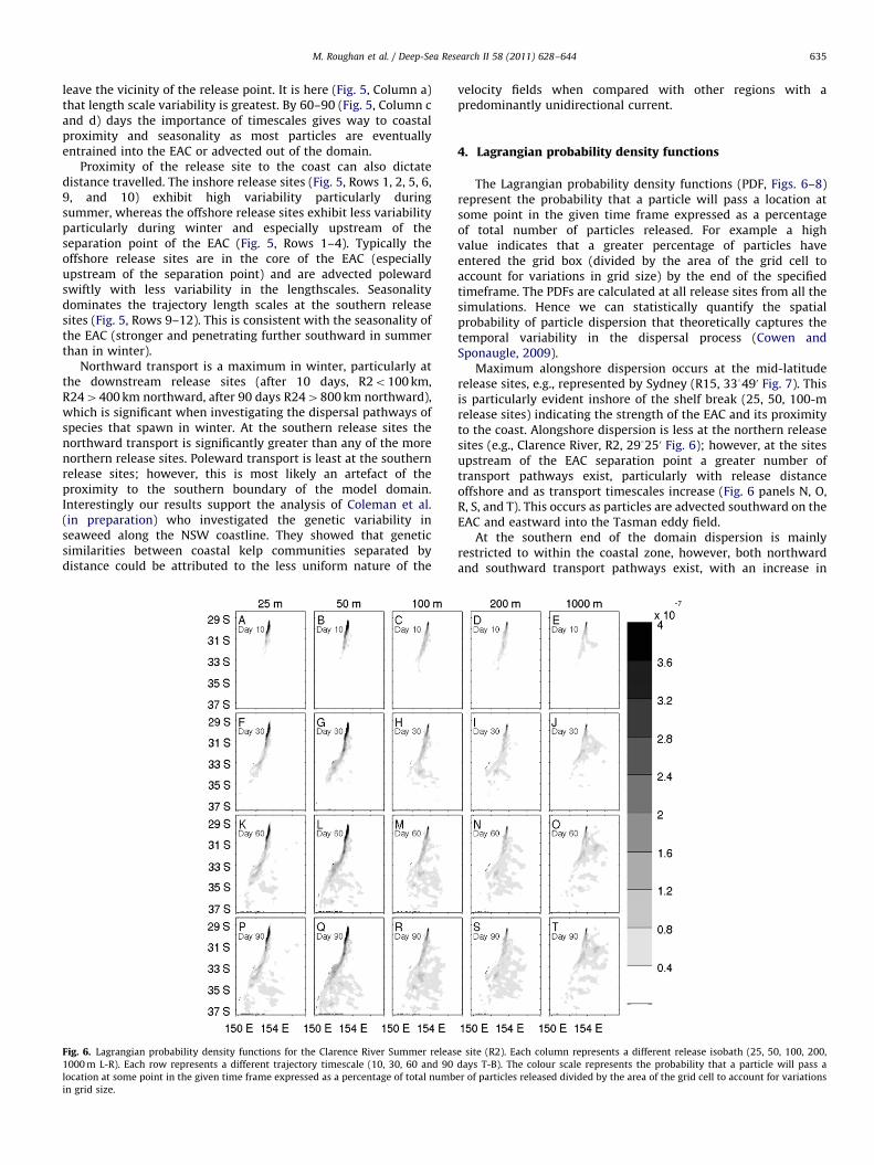
Fig. 6. Lagrangian probability density functions for the Clarence River Summer releas

1000 m L-R). Each row represents a different trajectory timescale (10, 30, 60 and 90

location at some point in the given time frame expressed as a percentage of total numb

in grid size.

velocity fields when compared with other regions with apredominantly unidirectional current.

4. Lagrangian probability density functions

The Lagrangian probability density functions (PDF, Figs. 6–8)represent the probability that a particle will pass a location atsome point in the given time frame expressed as a percentageof total number of particles released. For example a highvalue indicates that a greater percentage of particles haveentered the grid box (divided by the area of the grid cell toaccount for variations in grid size) by the end of the specifiedtimeframe. The PDFs are calculated at all release sites from all thesimulations. Hence we can statistically quantify the spatialprobability of particle dispersion that theoretically captures thetemporal variability in the dispersal process (Cowen andSponaugle, 2009).

Maximum alongshore dispersion occurs at the mid-latituderelease sites, e.g., represented by Sydney (R15, 33349u Fig. 7). Thisis particularly evident inshore of the shelf break (25, 50, 100-mrelease sites) indicating the strength of the EAC and its proximityto the coast. Alongshore dispersion is less at the northern releasesites (e.g., Clarence River, R2, 29325u Fig. 6); however, at the sitesupstream of the EAC separation point a greater number oftransport pathways exist, particularly with release distanceoffshore and as transport timescales increase (Fig. 6 panels N, O,R, S, and T). This occurs as particles are advected southward on theEAC and eastward into the Tasman eddy field.

At the southern end of the domain dispersion is mainlyrestricted to within the coastal zone, however, both northwardand southward transport pathways exist, with an increase in

e site (R2). Each column represents a different release isobath (25, 50, 100, 200,

days T-B). The colour scale represents the probability that a particle will pass a

er of particles released divided by the area of the grid cell to account for variations

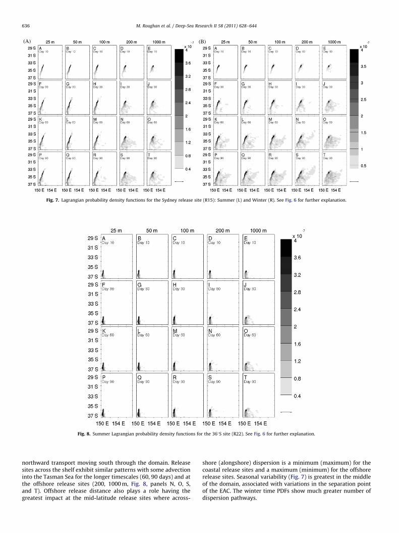
Fig. 7. Lagrangian probability density functions for the Sydney release site (R15): Summer (L) and Winter (R). See Fig. 6 for further explanation.

Fig. 8. Summer Lagrangian probability density functions for the 361S site (R22). See Fig. 6 for further explanation.

M. Roughan et al. / Deep-Sea Research II 58 (2011) 628–644636

northward transport moving south through the domain. Releasesites across the shelf exhibit similar patterns with some advectioninto the Tasman Sea for the longer timescales (60, 90 days) and atthe offshore release sites (200, 1000 m, Fig. 8, panels N, O, S,and T). Offshore release distance also plays a role having thegreatest impact at the mid-latitude release sites where across-

shore (alongshore) dispersion is a minimum (maximum) for thecoastal release sites and a maximum (minimum) for the offshorerelease sites. Seasonal variability (Fig. 7) is greatest in the middleof the domain, associated with variations in the separation pointof the EAC. The winter time PDFs show much greater number ofdispersion pathways.

Fig. 9. The PDF anomaly when comparing 700 and 50,000 particles released at each site for R2, R15 and R22 during Summer. Solid (dotted) line represents a 0.25 negative

(positive) difference.

M. Roughan et al. / Deep-Sea Research II 58 (2011) 628–644 637

4.1. Sensitivity to number of particles

To investigate the effects of diffusion, additional particletracking experiments were conducted over a 30-day period withvarying numbers of particles. Ten particles were released every30 min over a 30-day period (giving a total of 208,000 particlesper site) and were advected for 30 days. Two other scenarios wereinvestigated where 10 particles were released every 60 and120 min resulting in � 104,000 and � 52,000 particles per site.Results of the high density particle tracking experiments showthat an increased number of particles creates a somewhatsmoother PDF; however, the differences are not significant whenestimating circulation pathways (Fig. 9). In general PDF patternsare very similar, exhibiting southward flow which tends eastwardnear 311S. The greatest difference occurs at the EAC separationpoint, which is to be expected as this is a highly dynamic region(Fig. 9). However, this result does not affect the generalconclusions of this paper. Releasing more than 52,000 particlesmakes virtually no difference to the results. These results are inagreement with Griffa et al. (2004) who investigated the impact ofsmoothing of Eulerian velocity fields on the predictability ofLagrangian particles. The results show that the smoothing has astrong effect on the centre of mass behaviour, while the scatteraround it is only partially affected. Furthermore the impact onconnectivity results is minimal. We see a small increase in thenumber of connected estuaries where releasing more particlesallows for a slightly greater range in connectivity. There is also anincrease in connectivity to the north of some of the southernrelease sites suggesting that the experiments performed do notfully capture the variable nature of the northward flow. However,these two results do not impact on the general conclusions of thispaper, in fact they serve to support the results.

5. Connectivity

Connectivity matrices are a useful tool for describing thesource-to-destination relationships for larval dispersal over agiven larval development timeframe (Mitarai et al., 2008). Theyhave been used in recent times to diagnose the timespacedynamics of larval settlement (Cowen et al., 2006; Bode et al.,2006; Xue et al., 2008; Mitarai et al., 2009). Cowen and Sponaugle(2009) define a connectivity matrix as the probability of exchangeof individuals between patches. Here we column normalisethe matrix, hence the matrix elements rij gives the probabilitythat an individual released from population i will go to populationj. Hence in Figs. 10–12 the x-axis represents the source over the

given isobath and the y-axis represents the sink latitude at thecoast.

5.1. Mean connectivity and seasonal variability

Larval connectivity is inherently an intermittent and hetero-geneous process on annual timescales (Siegel et al., 2008). Thestochastic nature results primarily from the dependence of larvaeon coastal currents for advection. This creates an unavoidableuncertainty when trying to estimate the connectivity of popula-tions (Siegel et al., 2008). The advantage of a high-resolutionhindcast such as that used here, is that it can build a reliable viewof mean connectivity. Not only can we describe the connectivitywithin any single ‘realisation’ from year to year (1992–2006) andfrom season to season, (as per Section 5.2, following) whereconnectivity can vary significantly between realisations. Moreimportantly, we can now begin to quantify the variability in thesystem using our hindcast model. Figs. 10–11 show the seasonalvariability. The standard deviations of the connectivity matricesare also calculated for each scenario (not shown).

As identified in the particle trajectories and the Lagrangianprobability density functions (Figs. 4–8) typically upstream of theEAC separation point particles tend to be advected poleward bythe EAC. This affects the connectivity to the point that each regiontends to be connected to areas downstream of it (Figs. 10–11).

Also affecting the connectivity is the proximity of the releasesite to the coast. Particles released inshore of the EAC jet (typically25, 50 m) exhibit greater coastal connectivity than those releasedoffshore of the EAC front (Figs. 10–11, Rows 1, 2, and 3). The coreof the EAC generally flows above the 200-m isobath, but extendsout towards the 2000-m isobath, and is typically less than 100 kmwide. The separation point of the EAC (black line in matrices) alsodictates connectivity with more sites being connected (with lowerconcentration) downstream of the separation point of the EAC.

Particles released at the offshore sites (100–1000 m isobaths(Figs. 10–11, Rows 4 and 5) become quickly entrained in the EACjet. This combined with the greater distance from the shore meansthat of the particles released offshore, fewer reach the coast. Thisis exemplified by the lower number of connectivities. Theparticles that do reach the shore tend to have travelled greaterdistances (hence arrive further south) than particles releasedadjacent to the coast (e.g., Fig. 10, Panel Q, R).

Maximum number of sites that are connected (Table 2) occurredfor particles released at the 50-m isobath during summer (Fig. 10,Row 2, 32%). Whereas during winter, the maximum number of siteswere connected originated at the 100-m isobath (Table 2, 39%,

R1

→R

24

sink

29S

31S

37S

R1

→R

24

sink

29S

31S

37S

R1

→R

24

sink

29S

31S

37S

Log

%

R1

→R

24

sink

29S

31S

37S

R1

→R

24

sink

29S

31S

37S

R1 → R24

source29S

31S

37S

R1 → R24

source

29S

31S

37S

R1 → R24

source

29S

31S

37S

R1 → R24

source

29S

31S

37S

Fig. 10. Mean summer connectivity matrices: showing the relationship between particle sources and particle sinks along the coast of SE Australia given as a percentage of

total particles released from any given source. Particles were released in the surface waters at the 25, 50, 100, 200 and 1000 m isobaths (top to bottom) and connectivities

were calculated after 10, 30, 60 and 90 days (left to right). R1–R24 represent the release sites (from north–south) as identified in Table 1. The dashed line represents

‘self-connectivity’ and boxes above (below) the line represent southerly (northerly) transport.

M. Roughan et al. / Deep-Sea Research II 58 (2011) 628–644638

Fig. 11, Row 3) after 90 days. The total number of particles settled isa maximum for the coastal release sites (25-m isobath) duringsummer and winter (Figs. 10–11, Row 1) across all trajectorydurations, although dispersion is lower, indicated by the number ofsites that are connected. Trajectory timescales do play a role withthe maximum increase in the number of connectivities associatedwith the offshore release sites (Summer, 100, 200-m isobaths, 10%,winter 200, 1000-m isobaths, 21%). This indicates that it takeslonger for particles released at the offshore sites to return to shore.However, the actual number of particles settled decreases by anorder of magnitude from the coastal release site to the shelf breakrelease site. The pertinent result is that the majority of theopportunities for connectivity occur in the first 30 days and thatthe EAC acts as a barrier between onshore and offshore populations.The standard deviations are calculated for Figs. 10–11 (not shown)revealing that the variability is inversely proportional to theconnectivity.

5.2. Climatic controls on connectivity

The advantage of the downscaling method used is that itallows us to investigate the connectivity patterns for specificmonths or years. We can then begin to understand the impact ofthe EAC and climatic controls on the connectivity of populations(Fig. 12). The 1997–1998 El Nino was classified as strong to verystrong in the Australasian region, with very high SST anomaliesand a strong southern oscillation index (SOI). The SST anomaliesalong the east coast of Australia were as high as +2–3 1C, and theEAC jet was located well offshore. The location of the EAC jetobviously affects the transport pathways and hence the con-nectivity of populations (Fig. 12, Left panels). In contrast to thisperiod, December 1999 was a typical summer-time La Ninaperiod.

On average during December 1999 (La Nina) the total numberof connectivities was more than double that during the December

R1

→R

24

sink

29S

31S

37S

R1

→R

24

sink

29S

31S

37S

R1

→R

24

sink

29S

31S

37S

Log

%

R1

→R

24

sink

29S

31S

37S

R1

→R

24

sink

29S

31S

37S

R1 → R24

source29S

31S

37S

R1 → R24

source

29S

31S

37S

R1 → R24

source

29S

31S

37S

R1 → R24

source

29S

31S

37S

Fig. 11. Mean winter connectivity matrices. Description as per Fig. 10. Note the greater number of coloured boxes below the dashed line (indicating greater northward

transport) compared to the summer connectivity matrices (Fig. 10).

M. Roughan et al. / Deep-Sea Research II 58 (2011) 628–644 639

1997 El Nino period, but the number of connectivities did notincrease after 30 days, i.e. trajectory duration past 30 days playedno role. This is indicative of the poleward flow adjacent to thecoast. However, for the December 1997 case (El Nino), while onaverage the total number of connectivities was 50% less thanduring the La Nina period, a small number of new connectivitiesoccurred after 60 days. During the La Nina period a greaternumber of coastal sites received particles and a number ofparticles released at the 200-m isobath were returned to shore(La Nina (31 connected sites), El Nino (six connected sites)). Inboth years very few particles released at the 1000-m isobathreturned to shore, however, there were a greater number ofconnected sites during the La Nina (7) than the El Nino (3).

To investigate the general nature of these results, correlationswere calculated between the SOI and coastal connectivities overeach of the summer and winter periods studied. It was found thaton average during El Nino summers (where the EAC jet wastypically stronger and further offshore) connectivities were low(negative correlation with SOI), where as during La Nina summersmore particles were returned to the coast, particularly from

offshore sites (positive correlation with SOI). During Winterperiods, however, the converse scenario occurred with morecoastal connectivities during El Nino (negative SOI) periods. Thisperhaps indicates that the EAC jet was stronger and penetratedfurther southward than during a typical winter. This could alsohave implications for range extension of species (discussedfurther below).

While connectivity appears to be more significant during LaNina summer periods, it is possible that these differences are lessrelated to climatic variability and more a result of the dominationof the coastal circulation by the EAC eddy field. The relationshipbetween climatic variability and the EAC eddy field is an area forfurther investigation.

5.3. Particle source locations

Additional high-resolution simulations were run to correspondwith September of 2004. With a large number of particlesreleased, the source of particles to a particular location can be

25 m

Day 10 Day 30 Day 60 Day 90

50 m

100 m L

og

%

200 m

1000 m

source source source source

25 m

Day 10 Day 30 Day 60 Day 90

50 m

100 m L

og

%

200 m

1000 m

source source source source

Fig. 12. Summer connectivity matrices for December 1997 (L) and December 1999 (R): showing the relationship between particle sources and particle sinks along the coast

of SE Australia given as a percentage of total particles released from any given source. Particles were released in the surface waters at the 20, 50, 100, 200 and 1000 m

isobaths (top to bottom) and connectivities were calculated after 10, 30, 60 and 90 days (left to right).

Table 2The connectivities of all sites (%) and the number of particles settled (%) during summer and winter for timescales of 10, 30, 60 and 90 days (columns) at each isobath

release (rows).

Summer Winter

10 30 60 90 Incr. 10 30 60 90 Incr.

Estuaries connected at 25 m 17 19 20 20 3 16 20 20 21 5

Particles settled at 25 m 74 76 76 76 77 81 81 81

Estuaries connected at 50 m 25 30 32 32 7 19 26 28 31 12

Particles settled at 50 m 57 59 60 60 46 54 55 55

Estuaries connected at 100 m 21 28 30 31 10 19 30 36 39 20

Particles settled at 100 m 24 27 28 28 16 25 27 27

Estuaries connected at 200 m 11 18 20 21 10 8 19 25 29 21

Particles settled at 200 m 4.5 7.1 7.5 7.6 4.6 9.7 11 11

Estuaries connected at 1000 m 2 6 8 10 8 3 11 19 24 21

Particles settled at 1000 m 0.7 2.0 2.3 2.5 1.4 4.4 5.8 6.3

Incr. represents the increase in number of connected sites (as a % of the total allowable number of connections) from 10 days to 90 days, indicating the relative importance

of trajectory duration.

M. Roughan et al. / Deep-Sea Research II 58 (2011) 628–644640

investigated. This serves as an opportunity to aid in theinterpretation of ship board larval fish surveys that were under-taken at the Tasman Front during September 2004 (Mullaneyet al., submitted for publication; Baird et al., 2008). Particletracking simulations (Fig. 14) show the source location of the 232particles (from a total of 121,500 released on the shelf) that arefound near the Tasman Front sampling site on 5 September 2004.Two sink regions are specified as purple and grey, north and southof the 18 1C isotherm.

Particles from mid-north coast took 2–7 days for directtransport to the northern sector of the Tasman Front. An earlierwave of particles from the mid-north coast was advected southwhen the poleward extension of the EAC was strong, and find

themselves back at the Front 15–32 days after release havingtravelled a long way to the south (Fig. 14, top histogram). Despitetravelling below 361S, they are found to the north of the 18 1Cisotherm.

There is an interesting gap in particles between the grey andpurple plumes. This water must not have been near the coastin the last 32 days. Further south, particles have arrived fromthe south coast (purple) about 15–32 days (Fig. 14, bottomhistogram). The particles at the Tasman Front originate fromcoastal releases at a variety of times and from much of the NSWcoast. Interestingly, no particles came from the Stockton Bightregion ð333S,152355uEÞ, an important nursery ground for larvalfish.

R2

R4

R6

R8

R10

R12

R14

R16

R18

R20

R22

sink

29S

31S

37S

R2

R4

R6

R8

R10

R12

R14

R16

R18

R20

R22

sink

29S

31S

37S

R2

R4

R6

R8

R10

R12

R14

R16

R18

R20

R2229S

31S

37S

source

Log

%

0.2

0.4

0.6

0.8

1

1.2

1.4

1.6

1.8

2

R2

R4

R6

R8

R10

R12

R14

R16

R18

R20

R2229S

31S

37S

source

0

2.5

5

7.5

10

12.5

15

17.5

20

22.5

25

Fig. 13. Mean summer (A) and winter (B) connectivity matrices and their standard deviations (C, D) for a particle released over the 100 m isobath, representing a PLD

of 60 days.

M. Roughan et al. / Deep-Sea Research II 58 (2011) 628–644 641

6. Discussion

Here we have implemented a new high resolution model of thecoastal ocean of SE Australia with fairly realistic temperature andsalinity fields, producing a high resolution hindcast of the oceanstate (Baird et al., submitted for publication). This has the benefitsof high resolution adjacent to the coast, and across small scalefeatures, such as the Tasman Front. It is also advantageous in thatwe can include online particle tracking algorithms at high temporalresolution which is not possible from the BRAN output alone. Thedisadvantage of this method is that it is computationally intensive.We can use these simulations to investigate species specificdispersal pathways and as a baseline for future change scenarios.

6.1. Species-specific dispersal pathways

With the high-resolution hind cast model that we use in thisstudy, we now have the ability to construct species specific andspatially explicit models to describe connectivity. Neira and Keane(2008) highlight the importance of linking high resolutionoceanographic data with the spatio-temporal characteristics ofichthyoplankton spawning. Hence one of the aims of this study isto investigate how dispersal pathways (particle trajectories) differseasonally, inter-annually, with latitude and distance offshore.These variables go part of the way towards distinguishing thedispersal pathways of different larval species. We make use of theparticle trajectories calculated for four specific durations, 10, 30,60 and 90 days, which will provide indicative information for awide range of marine species.

In this section we relate the simulated particle paths to the fivelarval species that were introduced in Section 2.8. All the speciesare known to spawn in the Austral summer along this coastline,(except blue mackeral which spawns in winter and C. maenas

which spawns in both seasons) so the seasonal connectivitymatrices are appropriate. The various scenarios identified here aresummarised in Table 3.

6.1.1. Damselfish

For the tropical species we consider release sites from the100-m isobath offshore. While they spawn in shallow reefenvironments, if they are advected out of the Great Barrier Reefregion southward into our domain we assume that they havetravelled southward in the core of EAC which typically lies overthe shelf break. The connectivity results show that the 100 mrelease depth with a PLD of 30 days is very successful (Fig. 10J),with 21–28% of the sites connected, whereas offshore at the1000-m release depth only 2–6% of the sites are connected.

6.1.2. Butterflyfish

The results relevant to the butterflyfish exhibit similarpatterns to the damselfish, however, the extended PLD increasesthe probability of connectivity. It also increases the likelihood thatnorthern sites are connected with sites to the far south. Boothet al. (2007) have observed occurrences of butterflyfish along theNSW coastline as far south as 371S (R24), however, the moresouthern recruitment events tended to be much more episodicthan those at Sydney (33.81S, R15). Our mean matrices shows thaton average recruitment from releases at the most northern sites is

Temp [°C]

1414.51515.51616.51717.51818.51919.52020.52121.522

150 E 152 E 154 E 156 E 158 E

36 S

34 S

32 S

30 S

SEAPOM05-09-2004

1 m s-1

0 20 400

10

20

Cou

nts

0 20 400

10

20

Age

Cou

nts

153 E

34 S

Fig. 14. Particles arriving at 1531E (the Tasman Front) on 5 September 2004 from releases over the previous 32 days. Grey (purple) particle tracks are those found north

(south) of the 18 1C isotherm on 5 September. The insert magnifies the Front region for the 5th. The time since release of the particles is displayed as histograms in the top

left. The surface temperature is for 5 September, and the arrows trace the water moving from the 4th to 5th (i.e. distance in 1 day).

Table 3Criteria for determining species specific larval trajectory simulations and reference to the relevant connectivity matrix.

PLD (d) Trajectory duration (d) Release isobath (m) Spawning season Connectivity matrix

Damselfish 15–30 10, 30 100, 200, 1000 Summer Fig. 10I, J, M, N, Q, R

Butterflyfish 40–60 30, 60 100, 200, 1000 Summer Fig. 10J, K, N, O, R, S

Snapper 18–30 10, 30 25 Summer Fig. 10A, B

Blue mackeral 35 30 100, 200 Winter Fig. 11J, N

E. shore crab 30–40 30, 60 25, 50, 100 Summer Fig. 10B, C, F, G, J, K

E. shore crab 40–50 30, 60 25, 50, 100 Winter Fig. 11B, C, F, G, J, K

All particles were released in the surface waters above the corresponding isobath.

M. Roughan et al. / Deep-Sea Research II 58 (2011) 628–644642

possible at R15 (Sydney), but does not occur within 30 days at R24(Eden, 371S). By 60 days, however (butterflyfish) particles fromthe most northern sites have reached as far as 361S (R21)(Fig. 10K).

6.1.3. Snapper

The matrices relevant to snapper are the 25-m release sitewith a PLD of up to 30 days (Fig. 10A, B). By 30 days 19% of thesites are connected, however, most sites are connected to theiradjacent sites (typically downstream) with little alongshorespread. The maximum number of particles settle from thisinshore release site (76%) indicating that spawning over the25-m isobath with a PLD less than 30 days is a very successfulstrategy.

6.1.4. Blue mackeral

The blue mackeral (100, 200-m sites) spawn in winter (Fig. 11J, N)at the shelf break. Interestingly, during winter the 100-m release

depth is the most successful of all the across-shelf sites, with 30% ofsites being connected in the first 30 days. The 200-m site is lesssuccessful and the total number of particles settling is also lower(only 9.7%).

6.1.5. European shore crab

The first records of the European shore crab in NSW were fromthe southern end of our domain (Eden–Narooma) in the late1970s (Zeidler, 1978). Since this time it has been recorded from atotal of 20 estuaries or coastal lakes, many to the north (Ahyong,2005, Glasby unpubl. data). The invasion routes for most estuariesare unknown, but it is thought that C. maenas was oftentransported within NSW together with commercially grownoysters. Nevertheless, C. maenas has been found in numerousestuaries where there is no commercial oyster farming. Given thelong pelagic larval duration of C. maenas, it is quite likely thatcurrents may have played a role in the advection and subsequentinvasion of this species.

M. Roughan et al. / Deep-Sea Research II 58 (2011) 628–644 643

To investigate the dispersion of C. maenas we consider the coastalrelease sites, inshore of the 100-m isobath during both summer andwinter, for PLDs of 30–60 days (Figs. 10, 11B, C, F, G, J, K). Theconnectivity matrices in Fig. 13 indicate that estuaries in the vicinityof R20–R24 are well connected, particularly during winter and so itis quite likely that there could have been transport of C. maenas

larvae from south to north over distances of up to 200 km. Thestandard deviations in winter are relatively small at the southernend of the domain, suggesting that these patterns of connectivity areprecise. Of the sink sites that we modelled, R20–R24 have all hadreports of C. maenas occurring; however, oyster farms are notpresent. The results presented here indicate that northwardadvection by oceanic circulation is very possible. It is, however,unlikely that northward advection could explain the historicalrecords of C. maenas as far north as Sydney (R15).

The offshore release scenarios (200–1000 m) clearly show thatless than a handful of particles arrive at the coast. The fewparticles that do tend to reach the coast, do so after 30 days(summer) and 60 days (winter). These connectivities tend tooccur in coastal areas to the south of where the EAC has separatedfrom the coast. This has implications for the release of ballastwater and the potential spread of pests. The global practice ofdischarging ballast water from international vessels should beconsidered in relation to the potential onshore transport ofpropagules contained in the ballast water.

These results indicate exchange of ballast offshore in water atleast 200 m deep will indeed help minimise the chances of larvaearriving on the coast of SE Australia. But those larvae that couldarrive on the coast would likely do so a long distance from therelease point. Of the particles released at the 1000 m isobath, lessthan 2.5% are returned to the coast during summer and 6.3%during winter (Table 2). Furthermore, only 10% (24%) of the sitesare considered particle sinks after 90 days during summer(winter). This is in contrast to the 25-m release site where up to81% of particles are returned to the coast during winter. Theresults suggest that only those coastal species with long PLDs(460 days) would have a chance of being introduced via thisvector. These results therefore can help target surveys for newmarine pests that might arrive in ballast water that is beingdischarged offshore.

6.2. Range shifting and climate change

The work presented here gives a baseline from which we cannow assess the impacts of future changes in the East AustralianCurrent and the relevance for the dispersion and transport ofparticles. It is anticipated that the EAC will strengthen andpenetrate further to the south as the current becomes warmer,and evidence of this has already been seen (Hill et al., 2008). Thiswill presumably transport species endemic to lower latitudes tohigher latitudes, resulting in a range shift as has been observed inthe urchin Centrostephanus rodgersii (Johnson et al., 2005).Changes in the velocity fields will result in potentially signifi-cantly different dispersion patterns particularly over seasonal andinter-annual timescales. While the mesoscale eddy field controlsthe dispersion patterns downstream of the EAC separation point,how this eddy field will change remains unclear.

6.3. Limitations

When considering a question such as the transport of particlesfrom a coastal region such as an estuary, (e.g., for the Europeanshore crab) very specific parameters need to be included in orderfor the simulation to be realistic. Clearly this study is just astarting point. There are various limitations to the study, and the

results must be interpreted with that in mind. The dominantdriving force along the coast of SE Australia is the EAC and itseddy field, which makes numerical simulations fairly straightfor-ward. However, factors which influence coastal circulation aremore complex and more numbered. For example, tidal circulationand local wind forcing are two key forcing mechanisms whichhave not been included in this study. Condie et al. (2006) showedthat in strong tidal regime, tidal currents moved larvae back andforth across the shelf, however, it was the lower frequencycurrents that were responsible for alongshore advection and nettransport. In the EAC region tidal currents are typically an order ofmagnitude smaller than lower frequency currents so it isanticipated that their influence will be small. However, at theentrance to an estuary, tidal pumping may result in entrainmentof particles for many tidal cycles, combined with the effects oflocal wind forcing, or topographic steering, particles may actuallynever be able to leave the estuary and reach the open ocean.Observations have shown that it is possible for certain species totravel long distances along the NSW coastline and in fact enterestuaries a long way to the south of their release point (e.g., Boothet al., 2007), which gives validity to our results. Moreover, it hasbeen well documented that the larvae of species such as theEuropean shore crab readily exit and re-enter estuaries (Queiroga,1996).

The results of this study are derived from oceanographiccirculation studies alone. Larval behaviour has not been includedexplicitly, nor have we considered mortality or fecundity.Including these processes could improve (or complicate) theresults further. Cowen et al. (2006) show the importance of theearly onset of active larval movement in mediating the dispersalpotential. Although this was not included explicitly in our modelsimulations, this is perhaps an important mechanism where bylarval dispersion is reduced. The low level of connectivity after30 days suggests that early onset of motility might be importantfor increasing coastal connectivity.

Studies which include small-scale high-resolution estuarinemodels nested inside larger scale-shelf circulation models are ongoing at this time, with the next phase to implement fullindividual-based models that include specific larval character-istics and behaviour. However, the issue raises many complex andchallenging problems that have not yet been resolved by theinternational modelling community.

Acknowledgments

A component of this research was commissioned by the NewSouth Wales Department of Industry and Investment to assistwith a marine pest risk assessment, using funding from theSydney Metropolitan Catchment Management Authority. We aregrateful to J.H. Middleton and his oceanography group at UNSWfor their role in the early model development. HM is supported byan APA. MR is partially funded through the Australian IntegratedMarine Observing System (IMOS)—an initiative of the AustralianGovernment being conducted as part of the National CollaborativeResearch Infrastructure Strategy. This is contribution no. 0042from the Sydney Institute of Marine Science.

References

Ahyong, S.T., 2005. Range extension of two invasive crab species in easternAustralia: Carcinus maenas (Linnaeus) and Pyromaia tuberculata (Lockington).Marine Pollution Bulletin 50, 460–462.

Aiken, C.M., Navarrete, S.A., Castillo, M.I., Castilla, J.C., 2007. Along-shore larvaldispersal kernels in a numerical ocean model of the central Chilean coast.Marine Ecology Progress Series 339, 13–24.

M. Roughan et al. / Deep-Sea Research II 58 (2011) 628–644644

Baird, M., Roughan, M., Macdonald, H., Oke, P.R. Downscaling an eddy-resolvingglobal model for the continental shelf off southeast Australia. OceanModelling, submitted for publication.

Baird, M.E., Timko, P.G., Middleton, J.H., Mullaney, T.J., Cox, D.R., Suthers, I.M.,2008. Biological properties across the Tasman Front off southeast Australia.Deep-Sea Research Part I: Oceanographic Research Papers 55 (11), 1438–1455.

Baird, M.E., Timko, P.G., Suthers, I.M., Middleton, J.H., 2006a. Coupled physical–biological modelling study of the East Australian Current with idealised windforcing. Part I: biological model intercomparison. Journal of Marine Systems59, 249–270.

Baird, M.E., Timko, P.G., Suthers, I.M., Middleton, J.H., 2006b. Coupled physical–biological modelling study of the East Australian Current with idealised windforcing. Part II: biological dynamical analysis. Journal of Marine Systems 59,271–291.

Blumberg, A.F., Mellor, G.L., 1987. A description of a three-dimensional coastalocean circulation model. In: Heaps, N. (Ed.), Three Dimensional Coastal OceanModels, vol. 4. American Geophysical Union, Washington, DC, p. 208.

Bode, M., Bode, L., Armsworth, P.R., 2006. Larval dispersal reveals regional sourcesand sinks in the Great Barrier Reef. Marine Ecology Progress Series 308, 17–25.

Booth, D.J., Figueira, W.F., Gregson, M.A., Brown, L., Beretta, G., 2007. Occurrence oftropical fishes in temperate southeastern Australia: role of the East AustralianCurrent. Estuarine, Coastal and Shelf Science 72, 102–114.

Botsford, L.W., Micheli, F., Hastings, A., 2003. Principles for the design of marinereserves. Ecological Applications 13, 25–31.

Brassington, G., Oke, P., Pugh, T., 2006. BLUElink operational ocean prediction inAustralia. Advances in Geosciences 5, 87–95.

Carlton, J.T., 1987. Patterns of transoceanic marine biological invasions in thePacific Ocean. Bulletin of Marine Science 41, 452–465.

Chu, P.C., Fan, C., 2003. Hydrostatic correction for sigma coordinate ocean models.Journal of Geophysical Research 108 (C6), 3206.

Coleman, M.A., Roughan, M., Connell, S.D., Gillanders, B.M., Kelaher, B.P., Steinberg,P.D. Continental-scale patterns of connectivity among populations of kelp.Science, in preparation.

Condie, S.A., Andrewartha, J.R., 2008. Circulation and connectivity on theAustralian North West Shelf. Continental Shelf Research 28, 1724–1739.

Condie, S.A., Mansbridge, J.V., Hart, A.M., Andrewartha, J.R., 2006. Transport andrecruitment of silver-lip pearl oyster larvae on Australia’s North West shelf.Journal of Shellfish Research 25.1, 179+.

Cowen, R.K., Paris, C.B., Srinivasan, A., 2006. Scaling of connectivity in marinepopulations. Science 311, 522–527.

Cowen, R.K., Sponaugle, S., 2009. Larval dispersal and marine populationconnectivity. Annual Review of Marine Science 1, 443–466.

Craig, P.D., Banner, M.L., 1994. Modeling wave-enhanced turbulence in the oceansurface layer. Journal of Physical Oceanography 24 (12), 2546–2559.

deRivera, C., Hitchcock, N., Teck, S., Steves, B., Hines, A.H., Ruiz, G., 2007. Larvaldevelopment rate predicts range expansion of an introduced crab. MarineBiology 150, 1275–1288.

Flather, R., 1976. A tidal model of the northwest European continental shelf.Memoires de la Societe Royale des Sciences de Liege 10, 141–164.

Fox, C.J., McCloghrie, P., Nash, R.D.M., 2009. Potential transport of plaice eggs andlarvae between two apparently self-contained populations in the Irish Sea.Estuarine, Coastal and Shelf Science 81, 381–389.

Gabric, A.J., Parslow, J., 1994. The bio-physics of marine larval dispersion. Factorsaffecting larval dispersion in the Central Great Barrier Reef. In: Smmarco, P.W.,Heron, M.L. (Eds.), Coastal and Estuarine Studies, vol. 45. AmericanGeophysical Union.

Gillanders, B.M., Elsdon, T.S., Roughan, M., 2010. Connectivity of estuaries.Functioning of Estuaries and Coastal Ecosystems. In: Wolanski, E., McLusky,D. (Eds.), Treatise on Estuarine and Coastal Science, vol. 7. Elsevier.

Glasby, T.M., Lobb, K., 2008. Assessing the likelihood of marine pest introductionsin Sydney estuaries: a transport vector approach. Final Report Series no. X.NSW Department of Primary Industries, Fisheries, 75pp.

Griffa, A., Piterbarg, L.I., Ozgokmen, T., 2004. Predictability of lagrangian particletrajectories: effects of smoothing of the underlying Eulerian flow. Journal ofMarine Research 62, 1–35.

Hill, K.L., Rintoul, S.R., Coleman, R., Ridgway, K.R., 2008. Wind forced low frequencyvariability of the East Australia Current. Geophysical Research Letters 35 (8).

Hoese, D.F., Bray, D.J., Allen, G.R., Paxton, J.R., Wells, A., Beesley, P.L., 2006.Zoological Catalogue of Australia. Fishes, vol. 35. CSIRO Publishing.

Huret, M., Runge, J.A., Chen, C., Cowles, G., Xu, Q., Pringle, J.M., 2007. Dispersalmodeling of fish early life stages: sensitivity with application to Atlantic cod inthe western Gulf of Maine. Marine Ecology Progress Series 347, 261–274.

Johannes, R.E., 1978. Reproductive strategies of coastal marine fishes in the tropics.Environmental Biology of Fishes 3, 65–84.

Johnson, C., Ling, S., Ross, J., Scoresby, S., Miller, K., 2005. Establishment of the long-spined urchin (Centrostephanus rodgersii) in Tasmania: first assessment of thepotential threats to fisheries. Technical Report, Fisheries Research Develop-ment Corporation, Hobart, Tasmania.

Kalnay, E., Kanamitsu, M., Kistler, R., Collins, W., Deaven, D., Gandin, L., Iredell, M.,Saha, S., White, G., Woollen, J., et al., 1996. The NCEP/NCAR 40-year reanalysisproject. Bulletin of the American Meteorological Society 77 (3), 437–471.

Kingsford, M.J., Atkinson, M.H., 1994. Increments in otoliths and scales: how theyrelate to the age and early development of reared and wild larval and juvenilePagrus auratus (Sparidae). Australian Journal of Marine and FreshwaterResearch 45, 1007–1021.

Largier, J.L., 2003. Considerations in estimating larval dispersal distances fromoceanographic data. Ecological Applications 13, 71–89.

Macdonald, H.S., Baird, M.E., Middleton, J.H., 2009. Effect of wind on continentalshelf carbon fluxes off southeast Australia: a numerical model. Journal ofGeophysical Research 114, C05016.

Marchesiello, P., McWilliams, J.C., Shchepetkin, A., 2001. Open boundary conditionfor long-term integration of regional oceanic models. Ocean Modelling 3, 1–20.

Marchesiello, P., Middleton, J.H., 2000. Modeling the East Australian Currentin the Western Tasman Sea. Journal of Physical Oceanography 30, 2956–2971.

Mellor, G.L., Yamada, T., 1982. Development of a turbulent closure modelfor geophysical fluid problems. Reviews of Geophysics and Space Physics 20,851–875.

Mitarai, S., Siegel, D., Watson, J.R., Dong, C., McWilliams, J.C., 2009. Quantifyingconnectivity in the coastal ocean with application to the southern CalifornianBight. Journal of Geophysical Research 114.

Mitarai, S., Siegel, D., Winters, K., 2008. A numerical study of stochasticlarval settlement in the California Current system. Journal of Marine Systems69 (3–4), 295–309.

Mullaney, T.J., Miskiewicz, A.G., Baird, M.E., Burns, P.T.P., Suthers, I.M., submittedfor publication. Entrainment of larval fish assemblages into the Tasman Frontregion from the East Australian Current and coastal New South Wales,Australia. Fisheries Oceanography.

Neira, F.J., Keane, J.P., 2008. Ichthyoplankton-based spawning dynamics of bluemackerel (Scomber australasicus) in south-eastern Australia: links to the EastAustralian Current. Fisheries Oceanography 17 (4), 281–298.

North, E.W., Schlag, Z., Hood, R.R., Li, M., Zhong, L., Gross, T., Kennedy, V.S., 2008.Vertical swimming behavior influences the dispersal of simulated oysterlarvae in a coupled particle-tracking and hydrodynamic model of ChesapeakeBay. Marine Ecology Progress Series 359, 99–115.

Oke, P.R., Brassington, G.B., Griffin, D.A., Schiller, A., 2007. The Bluelink ocean dataassimilation system (BODAS). Ocean Modelling 21, 46–70.

Oke, P.R., Middleton, J.H., 2001. Nutrient enrichment off Port Stephens: the role ofthe East Australian Current. Continental Shelf Research 21, 587–606.

Queiroga, H., 1996. Distribution of the crab Carcinus maenas (L.) (Decapoda,Portunidae) larvae over the continental shelf off northern Portugal in April1991. Journal of Plankton Research 18, 1981–2000.

Ridgway, K.R., Godfrey, J.S., 1997. Seasonal cycle of the East Australian Current.Journal of Geophysical Research 102, 22921–22936.

Roughan, M., Mace, A.J., Largier, J.L., Morgan, S.G., Fisher, J.L., 2005. Sub-surfacerecirculation and larval retention in the lee of a small headland: a variation onthe upwelling shadow theme. Journal of Geophysical Research 110 (C10027).doi:10.1029/2005JC002898.

Roughan, M., Middleton, J.H., 2002. A comparison of observed upwellingmechanisms off the east coast of Australia. Continental Shelf Research 22(17), 2551–2572.

Roughan, M., Middleton, J.H., 2004. On the East Australian current: variability,encroachment and upwelling. Journal of Geophysical Research 109 (C07003).doi:10.1029/2003JC001833.

Roughan, M., Oke, P.R., Middleton, J.H., 2003. A modelling study of theclimatological current field and the trajectories of upwelled particles inthe East Australian Current. Journal of Physical Oceanography 33 (12),2551–2564.

Ruiz, G.M., Carlton, J.T., Grosholz, E.D., Hines, A.H., 1997. Global invasions ofmarine and estuarine habitats by non-indigenous species: mechanisms,extent, and consequences. American Zoologist 37, 621–632.

Siegel, D.A., Kinlan, B.P., Gaylord, B., Gaines, S.D., 2003. Lagrangian descriptions ofmarine larval dispersion. Marine Ecology Progress Series 260, 83–96.

Siegel, D.A., Mitarai, S., Costello, C.J., Gaines, S.D., Kendall, B.E., Warner, R.R.,Winters, K.B., 2008. The stochastic nature of larval connectivity amongnearshore marine populations. Proceedings of the National Academy ofSciences of the United States of America 105 (26), 8974–8979.

Smagorinsky, J., 1963. General circulation experiments with primitive equations,1. The basic experiment. Monthly Weather Review 91, 99–164.

Smolarkiewicz, P.K., 1984. A fully multidimensional positive definite advectiontransport algorithm with small implicit diffusion. Journal of ComputationalPhysics 54, 325–362.

Xue, H., Incze, L., Xu, D., Wolff, N., Pettigrew, N., 2008. Connectivity of lobsterpopulations in the coastal Gulf of Maine. Part I: circulation and larval transportpotential. Ecological Modelling 210 (1–2), 193–211.

Zeidler, W., 1978. Note on the occurrence of the European shore crab Carcinusmaenas (Linn., 1958) in Australia. South Australian Naturalist 53, 11–12.