Deep Shear Wave Velocity Profiling in the Mississippi Embayment Using The

NEES Field Shaker

Brent L. Rosenblad Jianhua Li

University of Missouri - Columbia

Motivation

• Shear wave velocity profiles are critical input parameters in geotechnical earthquake analysis

• Many seismically vulnerable sites in U.S. and worldwide are located on deep soil deposits that are generally not well characterized.

• There is need to characterize soil profiles to greater depths than conventional 30 m profiles

– Active source studies limited to depths of tens of m

– Passive source increasing used for deeper studies

• With the advent of low frequency NEES field vibrator, a comprehensive comparison study of active and passive methods for deep Vs profiling (200 m and greater) is possible.

Objective

• Present some of the results from extensive field studies of active and passive surface wave methods performed in the Mississippi Embayment using the NEES equipment

– Highlight some limitations of common methods

Low-Frequency Shaker (Liquidator)

120

100

80

60

40

20

0

For

ce,

kN

86420

Frequency, Hz

Conventional Vibroseis Liquidator

1.3 Hz

Custom built field shaker designed to address the problem of exciting energy in the frequency band of 5 Hz to less than 0.5 Hz.

Liquidator VibroseisReaction Mass

(kg)5900 1680

Stroke (cm) 40 10Peak Force (kN) 89 155

Force at 1Hz (kN)

48 3.3

Isolation Resonance (Hz)

0.3 1.5

Mississippi Embayment Study Area

Measurement Locations

• Many shallow Vs profiles (50 m or less)

•Very limited information about deeper deposits

•Objective was to determine profiles to 200 to 300 m depth

•Measurements performed at 11 sites (mostly CERI seismic stations)

General Site Geology

General Soil Conditions over Study Depth

•Alluvium (lowlands) and Loess (uplands)

•Vs~150 to 250 m/s

•thickness=10 to 60 m

•Silts and Clays (Eocene)

•Vs~350 to 450 m/s

•thickness=30 to 130 m

•Memphis Sand

•Vs~600 to 800 m/s

•thickness=200 m+

. . .

•Paleozoic Dolomite Depth of 500 to 900 m

Alluvium or Loess

Eocene Deposits

Memphis Sand

Surface Wave Methods

Active Source

• Spectral-Analysis-of-Surface-Waves (SASW) method – 2 channel approach

• Multi-channel method using f-k processing

Passive Source

• 2-D circular array and f-k processing

• Refraction Microtremor (ReMi) - passive energy with linear array

Steps in Surface Wave Analysis

• Data Collection– Sensor, # sensor, array configuration, frequencies, time or

frequency domain, source, source offset etc …

• Data Processing– Developing dispersion curve relating surface wave velocity versus

frequency or wavelength– Phase unwrapping (SASW), multi-channel transformations

• Forward Modeling/Inversion– Match a theoretical dispersion curve to the measured experimental

dispersion curve– Two approaches to forward modeling

• Modal dispersion curves (typical use fundamental mode)• Effective velocity dispersion curve

Field Testing Arrangement

Array 1 (L>150 m) Array 2 (L>300 m)

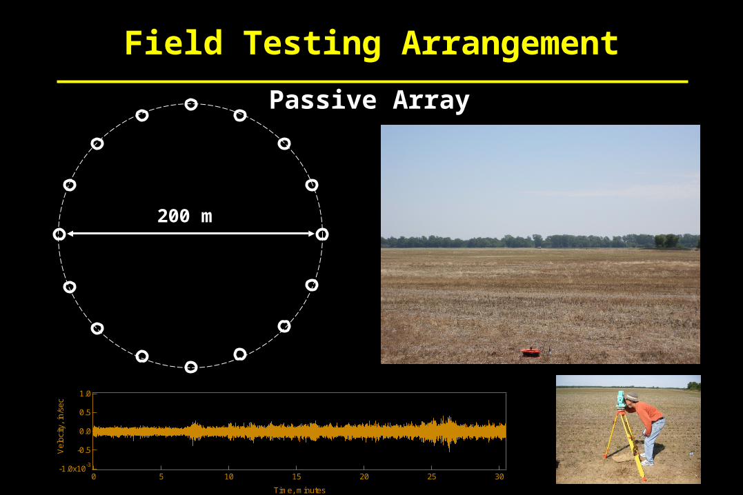
Field Testing Arrangement

Passive Array

200 m

-1.0x10-3

-0.5

0.0

0.5

1.0

Ve

loci

ty,

in/s

ec

302520151050

Time, minutes

SASW Method

Receiver Located 340 m from Source

-3

-2

-1

0

1

2

3

Pha

se, r

ad

3.02.52.01.51.0

Frequency, Hz

1.0

0.8

0.6

0.4

0.2

0.0

Coh

ere

nce

3.02.52.01.51.0

Frequency, Hz

Sample Data

• Uses the phase difference recorded

between a pairs of receivers with

receiver spacing, d, to determine the

effective surface wave velocity.

• The phase velocity at a given

frequency, f, is calculated from the

unwrapped phase difference, f, and

receiver spacing, d, using:

• Procedure is repeated for multiple

pairs of receivers to develop a

dispersion curve for the site

dφ

360fVR

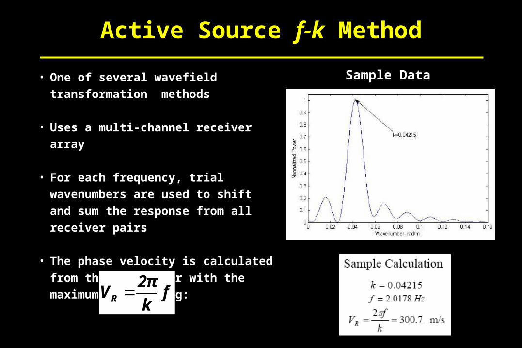
Active Source f-k Method

Sample Data• One of several wavefield transformation

methods

• Uses a multi-channel receiver array

• For each frequency, trial wavenumbers

are used to shift and sum the response

from all receiver pairs

• The phase velocity is calculated from the

wavenumber with the maximum power

using:

fk

2πVR

2-D Passive Array f-k Method

Peak

Sample Data

• Similar to 1-D approach but utilizes

a 2-D array (typically circular)

because the location of source is

not known

• For each frequency, trial kX and kY

values (velocity and direction) are

used to shift and sum the response

from all receiver pairs

• The phase velocity is calculated

from the wavenumber with the

maximum power using:f

2πVR k

kx (rad/m)

ky (

rad/

m)

-0.05 0 0.050.05-0.05

0

0.050.05

Refraction Microtremor (ReMi)

Slowness versus Frequency• Utilizes the slant stack (p- algorithm to develop a frequency-

slowness relationship

• A spectral ratio is calculated from

the power at a each frequency-

slowness point normalized by the

average power at that frequency

• Based on assumption that energy

impinges on array from all

directions

• Identifies likely phase velocity

values: peak, and middle “slope”

Measurement Issues

I. SASW phase unwrapping error

II. Fundamental mode inversion error

III. Wavefield assumption in ReMI

Example Dispersion Curve Comparison

800

600

400

200

0

Su

rfa

ce W

ave

Ve

loci

ty,

m/s

1086420

Frequency, Hz

SASW 1D fk (active source) 2D fk (passive source)

6004002000

Wavelength, m

ReMi-high ReMi-low ReMi-mid

I. SASW Phase Unwrapping Issue

200 m spacing

I. SASW Phase Unwrapping Issue

1 2

1 2

200 m spacing

II. Fundamental Mode Inversion

Site A : SASW/Effective

Site A : fk/fundamental Site B : fk/fundamental

Site B : SASW/Effective

Site A

Site A

Site B

Site B

Shear Wave Velocity Profiles

Site A Site B

Simulated fk and Modal Dispersion

Site A Site B

Soil Profiles at Sites A and B

Site A Site B

Simulated f-k: Synthetic Profile 1

Simulated f-k: Synthetic Profile 2

Simulated f-k: Synthetic Profile 3

III. Passive Wavefield Assumption

Example 2-D ReMi vs. Active Dispersion Comparison

III. Passive Wavefield Assumption

Example 2-D ReMi vs. Active Dispersion Comparison to 200 m

Passive Wavefield Characteristics

Freq=3.5 Hz Freq=1.6 Hz

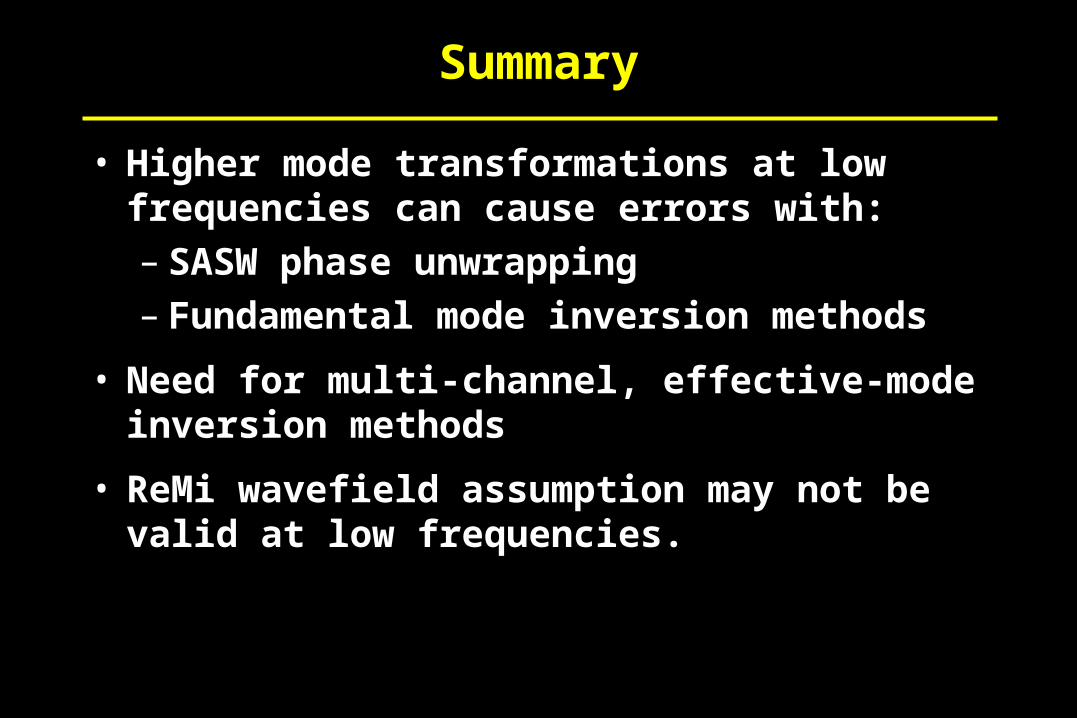
Summary

• Higher mode transformations at low frequencies can cause errors with:– SASW phase unwrapping – Fundamental mode inversion methods

• Need for multi-channel, effective-mode inversion methods

• ReMi wavefield assumption may not be valid at low frequencies.

Acknowledgements

This work was supported by: (1) grant No. 0530140 from the National Science Foundation as part of the Network for Earthquake Engineering Simulation (NEES) program, (2) USGS Award 06-HQGR0131.

The authors also thank personnel from :– Center for Earthquake Research and Information

(CERI) at University of Memphis for assistance in accessing the field sites.

– Prof. Van Arsdale at University of Memphis

– Personnel from NEES at Utexas field site