IEEE P

roof

1 Deep Trajectory Recovery with Fine-Grained2 Calibration using Kalman Filter3 Jingyuan Wang , Ning Wu, Xinxi Lu, Wayne Xin Zhao,Member, IEEE, and Kai Feng

4 Abstract—With the development of location-acquisition technologies, there are a huge number of mobile trajectories generated and

5 accumulated in a variety of domains. However, due to the constraints of device and environment, many trajectories are recorded at

6 low sampling rate, which increases the uncertainty between two consecutive sampled points in the trajectories. Our task is to recover

7 a high-sampled trajectory based on the irregular low-sampled trajectory in free space, i.e., without road network information. There

8 are two major problems with traditional solutions. First, many of these methods rely on heuristic search algorithms or simple

9 probabilistic models. They cannot well capture complex sequential dependencies or global data correlations. Second, for reducing

10 the predictive complexity of the unconstrained numerical coordinates, most of the previous studies have adopted a common

11 preprocessing strategy by mapping the space into discrete units. As a side effect, using discrete units is likely to bring noise or

12 inaccurate information. Hence, a principled post-calibration step is required to produce accurate results, which has been seldom

13 studied by existing methods. To address the above difficulties, we propose a novel Deep Hybrid Trajectory Recovery model,

14 named DHTR. Our recovery model extends the classic sequence-to-sequence generation framework by implementing a

15 subsequence-to-sequence recovery model tailored for the current task, named subseq2seq. In order to effectively capture

16 spatiotemporal correlations, we adopt both spatial and temporal attentions for enhancing the model performance. With the attention

17 mechanisms, our model is able to characterize long-range correlations among trajectory points. Furthermore, we integrate the

18 subseq2seq with a calibration component of Kalman filter (KF) for reducing the predictive uncertainty. At each timestep, the noisy

19 predictions from the subseq2seq component will be fed into the KF component for calibration, and then the refined predictions will be

20 forwarded to the subseq2seq component for the computation of the next timestep. Extensive results on real-world datasets have

21 shown the superiority of the proposed model in both performance and interpretability.

22 Index Terms—Trajectory recovery, sequence to sequence model, spatiotemporal attention, kalman filter

Ç

23 1 INTRODUCTION

24 WITH the popularization of GPS-enabled mobile devi-25 ces, a huge volume of trajectory data from users26 has become available in a variety of domains. These27 recorded trajectories provide an important kind of data28 signal to analyze, understand and predict mobile behav-29 iors. Many studies have shown that trajectory data is30 useful to improve the user-centric applications, includ-31 ing POI recommendation [1], urban planning [2], and32 route optimization [3].

33However, due to the constraints of device and environ-34ment, many trajectories are recorded at a low sampling rate.35As shown in previous studies [4], the low-sampled trajecto-36ries can not detail the actual route of objects, and increase37the uncertainty between two consecutive sampled points in38the trajectories. The high uncertainty significantly influences39related research that uses trajectory data, including trajec-40tory clustering [5], trajectory indexing [6], and trajectory41classification [7]. Trajectory recovery also has an important42impact on real-world applications, such as trip planning [8],43movement behavior study [9], [10] and traffic condition pre-44diction [11]. Hence, it is very important to develop effective45algorithms to recover high quality trajectories based on raw46low-sampled data.47Overall, the task of trajectory recovery has been stud-48ied in two different settings based on whether the map49information, such as road networks, is available or not50for use [9]. Under the first setting, the trajectory locations51are usually mapped to road segments [4], [12], [13], [14]52or Point-Of-Interests (POI) [15], [16], [17], [18], [19].53Then, the original trajectory recovery task will be simpli-54fied with such prior knowledge. While, under the second55setting, the map information is not available as input,56called free space trajectory recovery [9]. Comparing the two57settings, the latter is more challenging to solve but also58more common in practice. This work focuses on the sec-59ond setting.

� J. Wang is with the Beijing Advanced Innovation Center for Big Data andBrain Computing, School of Computer Science and Engineering, BeihangUniversity, Beijing 100191, China. E-mail: jywang@buaa.edu.cn.

� N. Wu and K. Feng are with the MOE Engineering Research Center ofAdvanced Computer Application Technology, School of Computer Scienceand Engineering, Beihang University, Beijing 100191, China.E-mail: {WuNing, fengkai}@buaa.edu.cn.

� X. Lu is with the School of Electronic and Information Engineering,Beihang University, Beijing 100191, China. E-mail: luxinxi@buaa.edu.cn.

� W.X. Zhao is with the School of Information, Renmin University of China,Haidian 100872, China, and also with the Beijing Key Laboratory of BigData Management and Analysis Methods, Beijing, China.E-mail: batmafly@gmail.com.

Manuscript received 11 Nov. 2018; revised 7 July 2019; accepted 1 Sept. 2019.Date of publication 0 . 0000; date of current version 0 . 0000.(Corresponding author: Wayne Xin Zhao.)Recommended for acceptance by W. Wang.For information on obtaining reprints of this article, please send e-mail to:reprints@ieee.org, and reference the Digital Object Identifier below.Digital Object Identifier no. 10.1109/TKDE.2019.2940950

IEEE TRANSACTIONS ON KNOWLEDGE AND DATA ENGINEERING, VOL. 31, NO. X, XXXXX 2019 1

1041-4347� 2019 IEEE. Personal use is permitted, but republication/redistribution requires IEEE permission.See ht _tp://www.ieee.org/publications_standards/publications/rights/index.html for more information.

IEEE P

roof

60 For solving the task of trajectory recovery, many efforts61 have been made in the literature. However, there are two62 potential problems with existing studies on the studied task.63 First, many of these methods rely on heuristic search algo-64 rithms or simple probabilistic models. They mainly model the65 adjacent transition patterns between locations, including66 depth-first search algorithm [4], [8], [20], absorbing Markov67 chain [21], andGibbs sampling [12].While, complex sequential68 dependencies or global data correlations can not be well cap-69 tured by these methods. Second, for reducing the predictive70 complexity of the unconstrained numerical coordinates, most71 of the previous studies have adopted a common preproce-72 ssing strategy by first mapping the space into discrete units,73 e.g., cells [8], [20] or anchor points [21], [22], [23]. Then, their74 focus becomes how to develop effective recovery algorithms75 over the discrete units. As a side effect, using discrete units is76 likely to bring noise or inaccurate information. Hence, a post-77 calibration step is usually required to produce more accurate78 results. While, previous methods mainly adopt simple heuris-79 tic calibrationmethods, e.g., identifying frequent locations in a80 cell [8], [20] or simply using the centric coordinates of the81 cell [21], [22], [23]. They have neglected the importance of post-82 calibration in refining the coarse unit-level prediction results.83 With the revival of neural networks, deep learning pro-84 vides a promising computational framework for solving85 complicated tasks. Many studies try to utilize the excellent86 modeling capacity for better learning effective characteris-87 tics from trajectory data. Especially, sequential neural mod-88 els, i.e., Recurrent Neural Networks (RNN), are widely89 used for modeling sequential trajectory data [24], [25], [26].90 Although these studies have improved the capacity of91 modeling complex sequential transition patterns to some92 extent, they only focus on next-step or short-term location93 prediction in a local time window. While, our task requires94 that the approach should be able to effectively model and95 utilize the global, comprehensive information from the96 entire trajectory. In addition, these studies still directly pro-97 duce the cell-level predictions, and do not incorporate a98 principled post-calibration component in their models for99 deriving more accurate estimations. Hence, it is difficult to

100 directly apply existing neural network based trajectory101 models to the task of free space trajectory recovery.102 To address the above difficulties, we propose a novelDeep103 Hybrid Trajectory Recovery model, named DHTR. Our recov-104 ery model substantially extends the classic sequence-105 to-sequence generation framework (i.e., seq2seq) by imple-106 menting a subsequence-to-sequence recoverymodel tailored107 for the current task, named subseq2seq. In order to effectively108 capture global spatiotemporal correlation, we adopt both109 spatial and temporal attentions for enhancing themodel per-110 formance. With the attention mechanisms, our model is able111 to characterize long-range correlations among trajectory112 points. Furthermore, we integrate the subseq2seq compo-113 nent with a Kalman Filter (KF) to calibrate noisy cell predic-114 tion as accurate coordinates. KF is widely used to deal with a115 series of measurements observed over time, containing sta-116 tistical noise and other inaccuracies. Different from conven-117 tional denoising applications that uses KF as an isolated118 postprocessing [27], we integrate the subseq2seq and KF in a119 joint deep hybrid model. Specifically, at each timestep, the120 noisy predictions from the subseq2seq component will be

121fed into the KF component for calibration, and then the122refined predictionswill be forwarded to the subseq2seq com-123ponent for the computation of the next timestep. In this man-124ner, our final model is endowed with the merits of both125components, i.e., the capacities of modeling complex126sequence data and reducing predictive noise.127Our contribution can be summarized as:

128� We propose a novel deep hybrid model by integrat-129ing subseq2seq with KF for trajectory recovery. To130our knowledge, it is the first time that deep learning131is integrated with KF for the studied task. By using a132hybrid of neural networks and KF, our model is133endowed with the benefits of both components, i.e.,134the capacities of modeling complex sequence data135and reducing predictive noise.136� As one of our major technical component, we extend137the classic seq2seq framework as the subseq2seq for138solving the current task. The subseq2seq approach139utilizes the elaborately designed spatiotemporal140attention mechanisms, which enhances the capacity141of modeling complex data correlations.142� We construct the evaluation experiments using three143real-world taxi trajectory datasets. Extensive results144on the three datasets have shown the superiority145of the proposed model in both effectiveness and146interpretability.

1472 RELATED WORKS

148Our work is closely related to the studies on trajectory149recovery and trajectory data mining. For trajectory recovery,150we further divide the related works into two categories,151using or not using road networks.

1522.1 Trajectory Recovery with Road Networks

153Given the information of road networks, previous studies154usually consider trajectory reconstruction as a route infer-155ence problem of mobile objects, persons or vehicles, moving156in a road network. The structure of road networks is used as157the prior knowledge or constraint of the route inference158algorithms. For example, Hsieh et al. propose to recom-159mend time-sensitive trip routes, consisting of a sequence of160locations associated with time stamps [16], [17]. Luo et al.161study a new path finding query which finds the most fre-162quent route during user specified time periods in large-scale163historical trajectory data [14]. In [4], a history based route164inference system (HRIS) has been proposed, which includes165several novel algorithms to perform the inference effec-166tively. Wu et al. propose a novel route recovery system in a167fully probabilistic way which incorporates both temporal168and spatial dynamics and achieve a state of art result [13].169Banerjee et al. employ Gibbs sampling by learning a Net-170work Mobility Model (NMM) from a database of historical171trajectories to infer the whole trajectories [12]. To fully uti-172lize the road network information, some studies involve a173preprocessing step calledmap matching [28], [29], [30], which174aligns location coordinates onto the road segments.175However, these studies highly rely on the structure of road176networks, which cannot work well in free space.

2 IEEE TRANSACTIONS ON KNOWLEDGE AND DATA ENGINEERING, VOL. 31, NO. X, XXXXX 2019

IEEE P

roof

177 2.2 Free Space Trajectory Recovery

178 Compared with the above works, free space trajectory179 recovery has no road network information as input. They180 usually try to identify the spatiotemporal patterns among181 adjacent location points, and reconstruct the trajectory using182 search based algorithms.183 For example, Chen et al. propose a Maximum Probability184 Product algorithm to discover the most popular route185 (MPR) from a transfer network based on the popularity186 indicators in a breadth-first manner [21]. Wei, Liu et al.187 build a routable graph from uncertain trajectories, and then188 answers a user’s online query (a sequence of point loca-189 tions) by searching top-k routes on the graph [8], [20]. These190 algorithms mainly consider simple adjacent transitions and191 correlations in a small region. They cannot model long-192 range or global correlations among location points in a193 trajectory.194 Especially, our work is also related to the works on trajec-195 tories similarity, since they usually involve trajectory recov-196 ery as an individual step before measuring the similarity.197 Su et al. propose an anchor-based calibration system that198 aligns trajectories to a set of anchor points [22]. Further-199 more, Su et al. propose a spatial-only geometry-based cali-200 bration approach that considers the spatial relationship201 between anchor points and trajectories [23].

202 2.3 Deep Learning for Trajectory Data Modeling

203 Recent years have witnessed the progress of deep learning204 in modeling complex data relations or characteristics. In205 specific, Recurrent Neural Network together with its variant206 Long Short-Term Memory (LSTM) have been widely used207 for modeling trajectory data. Zheng et al. propose a hierar-208 chical RNN to generate Long-term trajectories [24]. Wu209 et al. introduce a novel RNN model constrained by the road210 network to model trajectory [25]. Feng et al. design a multi-211 modal embedding recurrent neural network with historical212 attention to capture the complicated sequential transi-213 tions [26]. Chang et al. employ the RNN and GRU models214 to capture the sequential relatedness in mobile trajectories215 at different levels [31]. Liu et al. extend RNN and propose a216 novel method called Spatial Temporal Recurrent Neural217 Networks to predict the next location of a trajectory [32]. Al-218 Molegi et al. propose a novel model called Space Time219 Features-based Recurrent Neural Network (STF-RNN) for220 predicting people next movement based on mobility pat-221 terns obtained from GPS devices logs [33]. Most of these222 works mainly focus on modeling the sequence of location223 IDs rather than the numerical coordinate information.224 To our knowledge, there are very few studies that apply225 deep learning for trajectory recovery. Our work enhances226 the capacity of modeling complex trajectory sequences with227 neural networks, and further calibrates the predictions228 using the classic Kalman filter for reducing data noise. With229 the integration of Kalman filter, our predictive uncertainty230 is highly controlled.

231 3 PRELIMINARIES

232 In this section, we first introduce the notations throughout233 the manuscript, and then formally define our task.

234Definition 1 Location. A location or a location point is associ-235ated with a pair of coordinate values in the given geographical236space, measured by its latitude and longitude hx; yi.237Definition 2 Region cell.We assume that the entire geograph-238ical space is divided into a set of region cells (cell for short),239denoted by C. Each cell c 2 C is a square space with the length240of l, and corresponds to a centric location with the coordinates241of hxc; yci.242In practice, it is a common preprocessing technique to243transform the continuous measurements into discrete cells244as either main input [8], [21] or auxiliary data [22]. Using245cells is able to reduce the complexity of directly modeling246numerical coordinate sequence to some extent, since it is247easier to perform the computation over a discrete set of cell248IDs. We follow the procedure proposed in [20] for dividing249free geographical space into disjoint cells.

250Definition 3 Trajectory point. A trajectory point a (or b)251from an moving object is a timestamped location and modeled252by a quadruple hx; y; s; ci, where a:x is the longitude, a:y is the253latitude, a:s is the timestamp, and a:c is the cell that point a is254assigned to.

255Here, longitude and latitude are real numbers, a time-256stamp is accurate to seconds, and a cell is denoted by an257integer ID.

258Definition 4 Sampling interval. A sampling interval " is the259time difference between two consecutive sampled points for a260moving object, which usually depends on the device accurarcy.

261Definition 5 "-sampling trajectory. A "-sampling trajectory262t (trajectory for short) is a time-ordered sequence of n uniformly263sampled points from the same moving object using the sampling

264interval ". Formally, we have t ¼ aðtÞ1 ! a

ðtÞ2 ! . . .! aðtÞn .

265Given a "-sampling trajectory t, we have aðtÞiþ1:s� a

ðtÞi : s ¼

266" for 1 � i � n� 1 and aðtÞn :s� aðtÞ1 :s ¼ ðn� 1Þ". For simplic-

267ity, we omit the superscript of t in the notations of aðtÞi and

268use ai in the following content.

269Definition 6 "-sampling sub-trajectory. Given a "-sam-270pling trajectory t, a corresponding sub-trajectory ~t (sub-trajec-271tory for short) is a m-length subsequence of t. We have272~t ¼ b1 ! b2 ! . . .! bm, where bk ¼ ajk , 1 � j1 � � � � �273jm � n andm < n.

274Note that although the trajectory is uniformly sampled,275the locations in a sub-trajectory may not be uniformly dis-276tributed in timestamps. With the above definitions, ~t can be277equally written as aj1 ! aj2 ! . . .! ajm . We use the differ-278ent notations (i.e., ai and bk) for discriminating between a279trajectory and its corresponding sub-trajectories. Here, jð�Þ280can be considered as a mapping for transforming the cur-281rent indices of a sub-trajectory into the original indices of282the complete trajectory. It is easy to see that a trajectory can283correspond to multiple sub-trajectories by using different284mappings. Since the original trajectory is generated by uni-285formly sampling at each time interval ", we will have286bkþ1:s� bk:s ¼ ðjkþ1 � jkÞ".287Problem Statement. Given a "-sampling trajectory dataset288and a sub-trajectory ~t, we would like to reconstruct or289recover the corresponding trajectory t. That is to say, for

WANG ET AL.: DEEP TRAJECTORY RECOVERYWITH FINE-GRAINED CALIBRATION USING KALMAN FILTER 3

IEEE P

roof

290 each missing trajectory point ai (i.e., ai 2 t but ai =2 ~t), we291 will infer its corresponding longitude ai:x and latitude ai:y292 at time ai:s. The sampling interval " and time ai:s are293 assumed to be given as input. Such an assumption is ratio-294 nal since most of the measuring instruments sample the tra-295 jectory points regularly according to some fixed sampling296 interval. As aforementioned, the locations in a sub-trajec-297 tory may not be uniformly distributed in timestamps.298 Hence, our task is very challenging when road network is299 not available.

300 4 THE PROPOSED MODEL

301 In this section, we present the proposed Deep Hybrid Trajec-302 tory Recoverymodel, named as DHTR.

303 4.1 Overview

304 We first present an overview of the proposed model. Our305 model contains three major parts. The first is an elaborately306 designed subsequence-to-sequence (subseq2seq) neural network307 model. The subseq2seq component is developed on the clas-308 sic seq2seq model [34]. The second part is an attention309 mechanism, which is used to enable the subseq2seq to cap-310 ture the complex spatiotemporal correlations. Our attention311 mechanism considers both spatial and temporal influence312 among locations in an entire trajectory and therefore named313 as Spatiotemporal Attention. For reducing the complexity of314 directly modeling numerical coordinate sequences, the sub-315 seq2seq component captures the sequential relatedness at316 the cell level. In order to refine the coarse cell-level predic-317 tions, we enhance the subseq2seq model (See Section 4.4.1)318 with a novel post-calibration component based on Kalman319 filter in the third part. Instead of using a pipeline post-proc-320 essing approach, we integrate the subseq2seq component321 and the KF component in a joint deep hybrid model, which322 combines the merits of both components.323 We detail DHTR in an asymptotical way. In Section 4.2,324 we introduce the subseq2seq model for trajectory recovery.325 In Section 4.3, we incorporate the Spatiotemporal Attention326 into subseq2seq. Then, Section 4.4.1 provides the enhance-327 ment of the proposed model with the integration of Kal-328 man filter.

329 4.2 A Subseq2Seq Model for Trajectory Recovery

330 Instead of directly predicting the numerical coordinate val-331 ues, we first infer the corresponding cell of a missing trajec-332 tory point. In this manner, a sequence of trajectory points333 can be considered as a sequence of cell IDs. As shown334 in [24], it is more reliable and easy to model cell ID sequence335 than the original numerical sequence. Once the cell of a tra-336 jectory point can be inferred, we will use the the centric337 coordinate of the predicted cell to recover the missing loca-338 tion. In this way, our major task is how to recover the corre-339 sponding cell sequence using partial observations.

340 4.2.1 Motivation

341 In the standard seq2seq model [34] for sequence genera-342 tion, it consists of two major parts, namely encoder and343 decoder. The encoder is to map the input sequence to a344 fixed-sized vector using one RNN, and then the decoder is

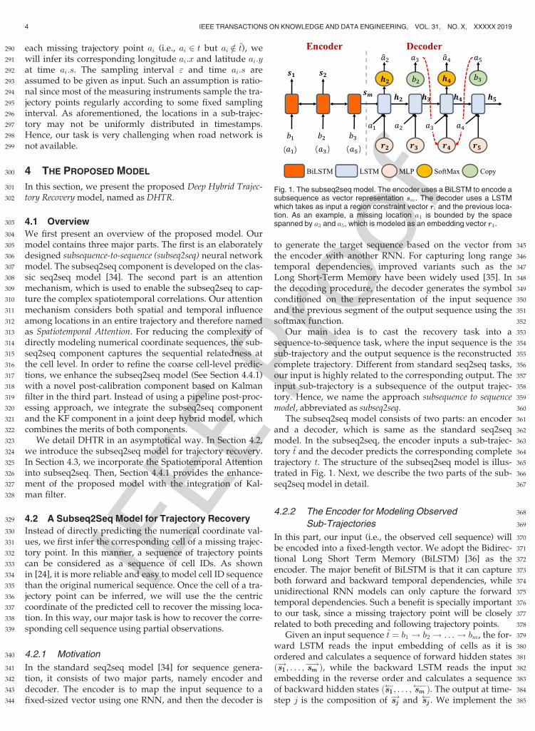
345to generate the target sequence based on the vector from346the encoder with another RNN. For capturing long range347temporal dependencies, improved variants such as the348Long Short-Term Memory have been widely used [35]. In349the decoding procedure, the decoder generates the symbol350conditioned on the representation of the input sequence351and the previous segment of the output sequence using the352softmax function.353Our main idea is to cast the recovery task into a354sequence-to-sequence task, where the input sequence is the355sub-trajectory and the output sequence is the reconstructed356complete trajectory. Different from standard seq2seq tasks,357our input is highly related to the corresponding output. The358input sub-trajectory is a subsequence of the output trajec-359tory. Hence, we name the approach subsequence to sequence360model, abbreviated as subseq2seq.361The subseq2seq model consists of two parts: an encoder362and a decoder, which is same as the standard seq2seq363model. In the subseq2seq, the encoder inputs a sub-trajec-364tory ~t and the decoder predicts the corresponding complete365trajectory t. The structure of the subseq2seq model is illus-366trated in Fig. 1. Next, we describe the two parts of the sub-367seq2seq model in detail.

3684.2.2 The Encoder for Modeling Observed

369Sub-Trajectories

370In this part, our input (i.e., the observed cell sequence) will371be encoded into a fixed-length vector. We adopt the Bidirec-372tional Long Short Term Memory (BiLSTM) [36] as the373encoder. The major benefit of BiLSTM is that it can capture374both forward and backward temporal dependencies, while375unidirectional RNN models can only capture the forward376temporal dependencies. Such a benefit is specially important377to our task, since a missing trajectory point will be closely378related to both preceding and following trajectory points.379Given an input sequence ~t ¼ b1 ! b2 ! . . .! bm, the for-380ward LSTM reads the input embedding of cells as it is381ordered and calculates a sequence of forward hidden states382ðs1s1!; . . . ; smsm

�!Þ, while the backward LSTM reads the input383embedding in the reverse order and calculates a sequence384of backward hidden states ðs1s1 ; . . . ; smsm

�Þ. The output at time-385step j is the composition of sjsj

! and sjsj . We implement the

Fig. 1. The subseq2seq model. The encoder uses a BiLSTM to encode asubsequence as vector representation ssm. The decoder uses a LSTMwhich takes as input a region constraint vector rri and the previous loca-tion. As an example, a missing location a4 is bounded by the spacespanned by a3 and a5, which is modeled as an embedding vector rr4.

4 IEEE TRANSACTIONS ON KNOWLEDGE AND DATA ENGINEERING, VOL. 31, NO. X, XXXXX 2019

IEEE P

roof

386 composition as the vectorized sum, and have the final repre-387 sentation ssj ¼ sjsj

!þ sjsj for the jth state of the input sequence.

388 4.2.3 The Decoder for Reconstructing Missing

389 Trajectories

390 Compared with the standard seq2seq application, our task391 has two unique characteristics, and we need to make suit-392 able adaptations for the decoder according to our task.393 First, the input is a subsequence of the output sequence394 in our task. In our model, for a known point from the input395 sequence, we apply the similar idea of “copy mechanism”396 from the NLP field [37] to directly generate the copy at the397 corresponding output slot. As shown in Fig. 1, in the pro-398 posed model, the copy mechanism is formulated as follows

ai ¼ ai; jk < i < jkþ1 (an unobserved point);bk; i ¼ jk (an observed point);

�(1)

400400

401 where ai denotes the prediction result using the decoder. In402 a word, we only predict the unobserved point, while the403 observed point is simply copied from the sub-trajectory.404 Second, as previous studies have shown [8], the trajec-405 tory recovery task can be effectively solved by searching406 related several local trajectory points. More specially, a sin-407 gle trajectory point is usually bounded in a local region. In408 Fig. 1, we present an illustrative example with such region409 constraints. An observed sub-trajectory consists of three410 points: a1, a3, and a5. The missing point a4 is likely to fall in411 the region spanned by its preceding point a3 and successive412 point a5. Hence, incorporating region constraint is impor-413 tant to trajectory reconstruction. Instead of using hard rules,414 we propose to use hidden representations for modeling415 such region constraints. Especially, we use an embedding416 vector rri to denote the constraint information for the ith tra-417 jectory point ai, defined as

rri ¼ DNNðajk ; ajkþ1Þ: (2)419419

420 where DNNð�Þ is a function consisting of an look-up layer421 and a Multi-Layer Perceptron (MLP), ajk and ajkþ1 are the422 observed precursor and successor for ai, and jk < i < jkþ1.423 In this way, the prediction of a point can utilize the informa-424 tion from its observed precursor and successor in a425 trajectory.426 To this end, for inferring a missing point, our decoder427 derives the hidden state hihi as

hihi ¼ LSTMðai�1; rri; hhi�1; ssmÞ: (3)429429

430 where rri is the region constraint vector defined in Eq. (2)431 and ssm is the output state derived from the encoder. Once432 we obtain the hidden state hhi from the decoder, we further433 apply the softmax function to generate the corresponding434 cell of the missing trajectory point conditioned on the proba-435 bility of PrðcjhhiÞ as

PrðcjhhiÞ ¼ expðhhi> � wwcÞP

c02C expðhhi> � wwc0 Þ

; (4)

437437

438 where wwc is the cth column vector from a trainable parame-439 ter matrixWWC .

4404.2.4 Applying the Model for Trajectory Recovery

441Given a training dataset D consisting of trajectory and sub-442trajectory pairs, we define the following objection function

L1 ¼Xht;~ti2D

�logPrðtj~tÞ; (5)

444444

445where Prðtj~tÞ is computed using the softmax following the446original seq2seq model using Eq. (4).447For applying the model to our task, at each timestep i, we448first infer the corresponding cell of a missing trajectory point,449namely bi:c. Then we use the centric coordinate of the cell bi:c450as the final predictions. In practice, for accuracy, we usually451set a small cell length, e.g., 100 � 200 meters. The complexity452for the subseq2seq model increases with the decreasing of the453cell length, since there will be more cells for predictions.454Hence, we need to make a trade-off between the above two455aspects for setting the cell length. We will discuss the effect of456the cell length on themodel performance in Section 5.3.3.

4574.3 Incorporating the Spatiotemporal Attention

458In the aforementioned subseq2seq model, we only consider459local region constraint, while long-range or global correla-460tions can not be modeled. Such correlations mainly reflect461the spatiotemporal influence among trajectory points [32],462which is more important to consider in free space without463using road networks. Next, we adopt the Spatiotemporal464Attention mechanism to capture the spatiotemporal influ-465ence among trajectory points.

4664.3.1 A Standard Attention Mechanism

467We first present a standard attention mechanism [34] for the468general seq2seq model by rewriting Eq. (3) as

hhi ¼ LSTMðai�1; rri; hhi�1; ssm; eeiÞ; (6)470470

471where the context vector eei is computed by a weighted sum472of these hidden states ss from the encoder

eei ¼Xmk¼1

ai;kssk: (7)

474474

475An important part is how to compute the attention coeffi-476cients fai;jg. Following [38], we can apply the softmax func-477tion to derive fai;jg as

ai;k ¼ expðui;kÞPmk0¼1 expðui;k0 Þ

; (8)479479

480

ui;k ¼ vv> � tanhðWWHhhi þWWSsskÞ; (9)

482482

483where vv, WWH and WWS are the parameter vector or matrices484to learn. This attention mechanism mainly captures the gen-485eral correlations among hidden states in the sequence.486While, in our task, we need to explicitly model spatiotempo-487ral influence with the attention mechanism.

4884.3.2 Modeling the Spatiotemporal Influence

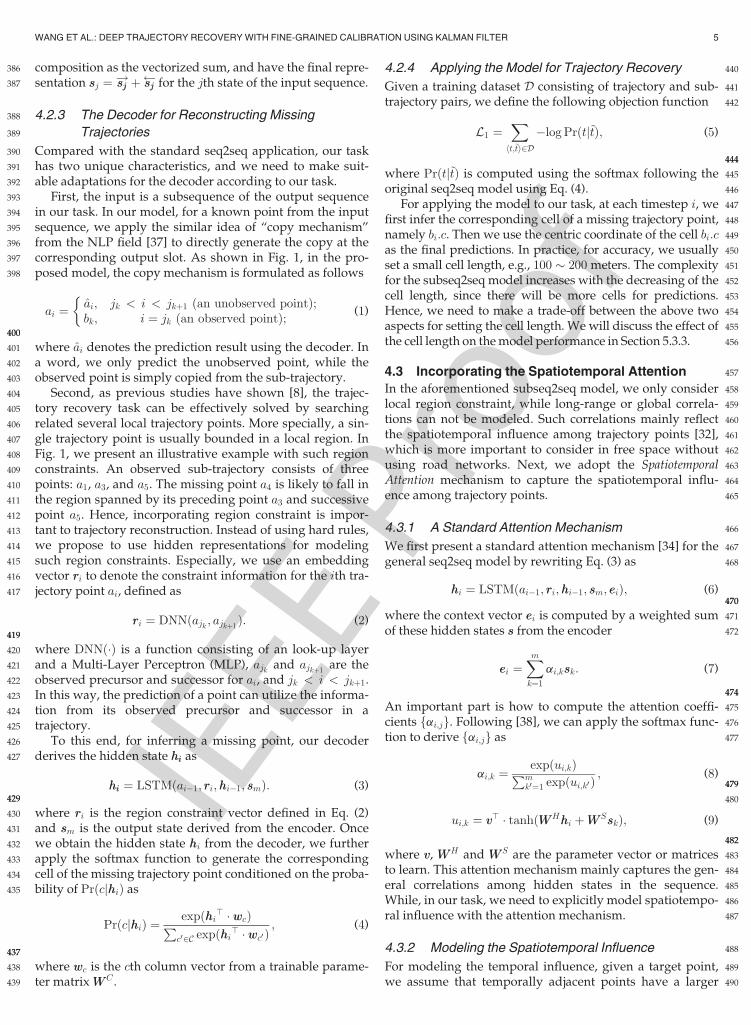
489For modeling the temporal influence, given a target point,490we assume that temporally adjacent points have a larger

WANG ET AL.: DEEP TRAJECTORY RECOVERYWITH FINE-GRAINED CALIBRATION USING KALMAN FILTER 5

IEEE P

roof

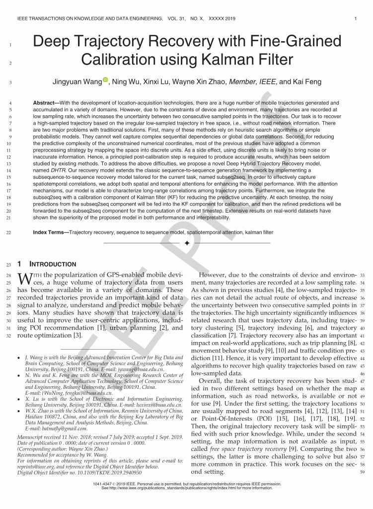
491 influence than temporally distant points in a trajectory. In492 other words, the influence decreases with the increasing of493 the temporal distance. Inspired by the method for modeling494 positional information from the NLP field [39], [40], [41],495 the temporal distance between the ith predicted point and496 kth observed point is defined as

dð1Þi;k ¼ jk � ij j: (10)

498498

499 We have presented an illustrative example in Fig. 2. Here500 d

ð1Þ1;5 ¼ 4 since there are four sample intervals between the

501 two trajectory points.502 Similarly, the spatial influence can be computed with the503 euclidean distance of locations as

dð2Þi;k ¼

ffiffiffiffiffiffiffiffiffiffiffiffiffiffiffiffiffiffiffiffiffiffiffiffiffiffiffiffiffiffiffiffiffiffiffiffiffiffiffiffiffiffiffiffiffiffiffiffiffiffiffiffiffiffiffiffiffiffiffiffiffiffiffiðajk :x� bi:xÞ2 þ ðajk :y� bi:yÞ2

q: (11)

505505

506 However, during the inferring process, we do not have the507 coordinate information of bi:x and bi:y, which are our goal508 to learn. Hence, we use the (inferred) coordinate informa-509 tion of the previous point to approximate the computation510 of d

ð2Þi;k . In the Eq. (11), d

ð2Þi;k is in a real number. We further

511 discretize the distance into integers via dividing dð2Þi;k by the

512 cell length.513 For a given trajectory, the scales of both d

ð1Þi;k and d

ð2Þi;k are

514 usually bounded in a limited small range. So we propose to515 associate each discretized value for each kind of distance516 with an embedding vector. Then, the spatial-temporal influ-517 ence is finally modeled as

ui;k ¼ vv> tanh WWHhhi þWWSssk þWWPppdð1Þi;k

þWWQqqdð2Þi;k

� �;

(12)519519

520 where fppg and fqqg are the embedding parameters corre-521 sponding to the temporal and spatial influences respec-522 tively, which are indexed by the discretized distance values

523 of dð1Þi;k and d

ð2Þi;k . The matricesWWP andWWQ are the parameters

to learn.

5244.4 Incorporating Kalman Filter

525Above, we first apply the subseq2seq model to characterize526the cell sequence for a trajectory, and then the centric coordi-527nate of the predicted cell is treated as the final prediction. The528approach has two potential shortcomings. First, the prediction529model is likely to be affected by noise, e.g., the instrumental530errors. Second, the final estimations are coarse since we use531the corresponding cell coordinate as a surrogate.532To address these issues, we propose to integrate the533above neural network model with Kalman filter. Kalman534Filter [42] is particularly useful in dealing with varying tem-535poral information. Especially, several studies have applied536the KF model to calibrate noisy estimates in object track-537ing [43]. Compared with sequence neural networks, the538standard KF is a linear system model, which can not capture539long-range temporal dependencies. To develop our appr-540oach, our idea is to combine the benefits of sequence neural541networks and KF with a hybrid model.

5424.4.1 The General Description of Kalman Filter

543Generally speaking, Kalman Filters (KFs) are optimal state544estimators under the assumptions of linearity and Gaussian545noise. In the KF model, we use a state vector ggi, which could546consists of the location and/or speed, to denote the state of547a mobile object at the time i. The object linearly updates the548state ggi with a Gaussian noise eeg as

ggi ¼ FFggi�1 þ eeg; eeg � Nð0;MMÞ; (13)550550

551where MM is the covariance of eeg, and FF is a state update552matrix. In the KF model, the real value ggi can be measured553by a measurement vector zzi as

zzi ¼ CCggi þ eez; eez � Nð0; NNÞ; (14)555555

556where CC is measurement matrix, eez is a Gaussian measure-557ment noise and NN is the covariance of eez. In the KF model,558the measurement vector zzi is observable, the real state ggi is559the unknown variable to be estimated. The matrices FF, CC,560MM, andNN in Eqs. (13) and (14) are known as a priori.561The KF model uses two procedures, Prediction and562Update, to iteratively estimate the true value of gg and calcu-563late a covariance matrix, denoted asHH, to express the uncer-564tainty of gg.565Prediction. In the prediction procedure, the KF model566uses following equations to predict the state gg and the567covariance matrixHH at the timestep i

ggiji�1 ¼ FFggi�1ji�1; (15) 569569

570

HHiji�1 ¼ FFHHi�1ji�1FF> þMM; (16)

572572

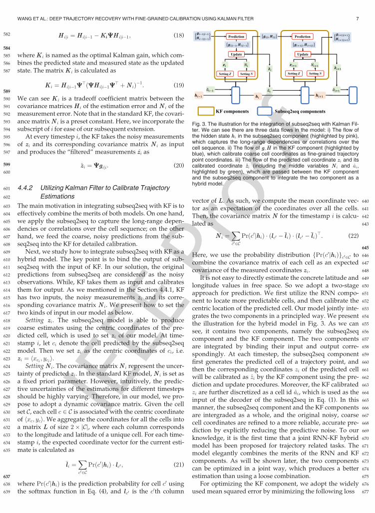
573where ggi�1ji�1 and HHi�1ji�1 with the subscript “i� 1ji� 1”574denotes the variables generated by the update procedure at575the timestep i� 1, while ggiji�1 and HHiji�1 with the subscript576“iji� 1” denotes the predicted state and covariance.577Update. In the update procedure, the KF model use the578observable measurement vector zzi to update/collate the579predicted ggiji�1 andHHiji�1 as

ggiji ¼ ggiji�1 þKKiðzzi �CCggiji�1Þ; (17) 581581

Fig. 2. The proposed spatiotemporal attention mechanism. Here, we aregiven a sequence of seven trajectory points from a1 to a6, where a1, a3,a4 and a6 (b2 and b5) are observed and the rest are for prediction. Forregion constraints, a5 is only bounded by the pair of a4 and a6. We alsoplot the computation for both the temporal and spatial influence of a1 toa5. Utilizing the attention mechanism makes it feasible to explore long-range correlations or dependencies.

6 IEEE TRANSACTIONS ON KNOWLEDGE AND DATA ENGINEERING, VOL. 31, NO. X, XXXXX 2019

IEEE P

roof

582 HHiji ¼ HHiji�1 �KiKiCCHHiji�1; (18)

584584

585 whereKKi is named as the optimal Kalman gain, which com-586 bines the predicted state and measured state as the updated587 state. The matrixKKi is calculated as

KKi ¼ HHiji�1CC>ðCCHHiji�1CC

> þNNiÞ�1: (19)589589

590 We can see KKi is a tradeoff coefficient matrix between the591 covariance matrices HHi of the estimation error and NNi of the592 measurement error. Note that in the standard KF, the covari-593 ance matrixNNi is a preset constant. Here, we incorporate the594 subscript of i for ease of our subsequent extension.595 At every timestep i, the KF takes the noisy measurements596 of zzi and its corresponding covariance matrix NNi as input597 and produces the “filtered” measurements zzi as

zzi ¼ CCggiji: (20)599599

600

601 4.4.2 Utilizing Kalman Filter to Calibrate Trajectory

602 Estimations

603 The main motivation in integrating subseq2seq with KF is to604 effectively combine the merits of both models. On one hand,605 we apply the subseq2seq to capture the long-range depen-606 dencies or correlations over the cell sequence; on the other607 hand, we feed the coarse, noisy predictions from the sub-608 seq2seq into the KF for detailed calibration.609 Next, we study how to integrate subseq2seq with KF as a610 hybrid model. The key point is to bind the output of sub-611 seq2seq with the input of KF. In our solution, the original612 predictions from subseq2seq are considered as the noisy613 observations. While, KF takes them as input and calibrates614 them for output. As we mentioned in the Section 4.4.1, KF615 has two inputs, the noisy measurements zzi and its corre-616 sponding covariance matrix NNi. We present how to set the617 two kinds of input in our model as below.618 Setting zzi. The subseq2seq model is able to produce619 coarse estimates using the centric coordinates of the pre-620 dicted cell, which is used to set zzi of our model. At time-621 stamp i, let ci denote the cell predicted by the subseq2seq622 model. Then we set zzi as the centric coordinates of ci, i.e.623 zzi ¼ hxci ; ycii.624 Setting NNi. The covariance matrix NNi represent the uncer-625 tainty of predicted zzi. In the standard KF model, NNi is set as626 a fixed priori parameter. However, intuitively, the predic-627 tive uncertainties of the estimations for different timesteps628 should be highly varying. Therefore, in our model, we pro-629 pose to adopt a dynamic covariance matrix. Given the cell630 set C, each cell c 2 C is associated with the centric coordinate631 of hxc; yci. We aggregate the coordinates for all the cells into632 a matrix LL of size 2� jCj, where each column corresponds633 to the longitude and latitude of a unique cell. For each time-634 stamp i, the expected coordinate vector for the current esti-635 mate is calculated as

�lli ¼Xc02C

Prðc0jhhiÞ � llc0 ; (21)

637637

638 where Prðc0jhhiÞ is the prediction probability for cell c0 using639 the softmax function in Eq. (4), and llc0 is the c0th column

640vector of LL. As such, we compute the mean coordinate vec-641tor as an expectation of the coordinates over all the cells.642Then, the covariance matrix NN for the timestamp i is calcu-643lated as

NNi ¼Xc02C

Prðc0jhhiÞ � ðllc0 ��lliÞ � ðllc0 ��lliÞ>: (22)

645645

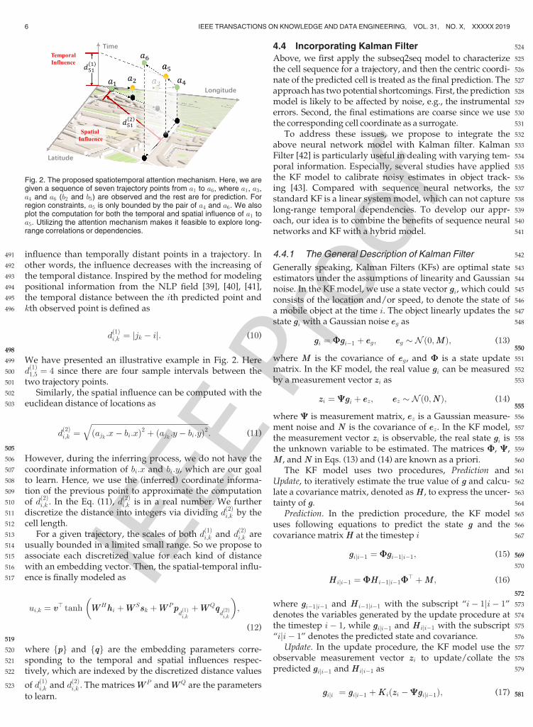
646Here, we use the probability distribution fPrðc0jhhiÞgc02C to647combine the covariance matrix of each cell as an expected648covariance of the measured coordinates zzi.649It is not easy to directly estimate the concrete latitude and650longitude values in free space. So we adopt a two-stage651approach for prediction. We first utilize the RNN compo-652nent to locate more predictable cells, and then calibrate the653centric location of the predicted cell. Our model jointly inte-654grates the two components in a principled way. We present655the illustration for the hybrid model in Fig. 3. As we can656see, it contains two components, namely the subseq2seq657component and the KF component. The two components658are integrated by binding their input and output corre-659spondingly. At each timestep, the subseq2seq component660first generates the predicted cell of a trajectory point, and661then the corresponding coordinates zi of the predicted cell662will be calibrated as zi by the KF component using the pre-663diction and update procedures. Moreover, the KF calibrated664zi are further discretized as a cell id ai, which is used as the665input of the decoder of the subseq2seq in Eq. (1). In this666manner, the subseq2seq component and the KF components667are intergraded as a whole, and the original noisy, coarse668cell coordinates are refined to a more reliable, accurate pre-669diction by explicitly reducing the predictive noise. To our670knowledge, it is the first time that a joint RNN-KF hybrid671model has been proposed for trajectory related tasks. The672model elegantly combines the merits of the RNN and KF673components. As will be shown later, the two components674can be optimized in a joint way, which produces a better675estimation than using a loose combination.676For optimizing the KF component, we adopt the widely677used mean squared error by minimizing the following loss

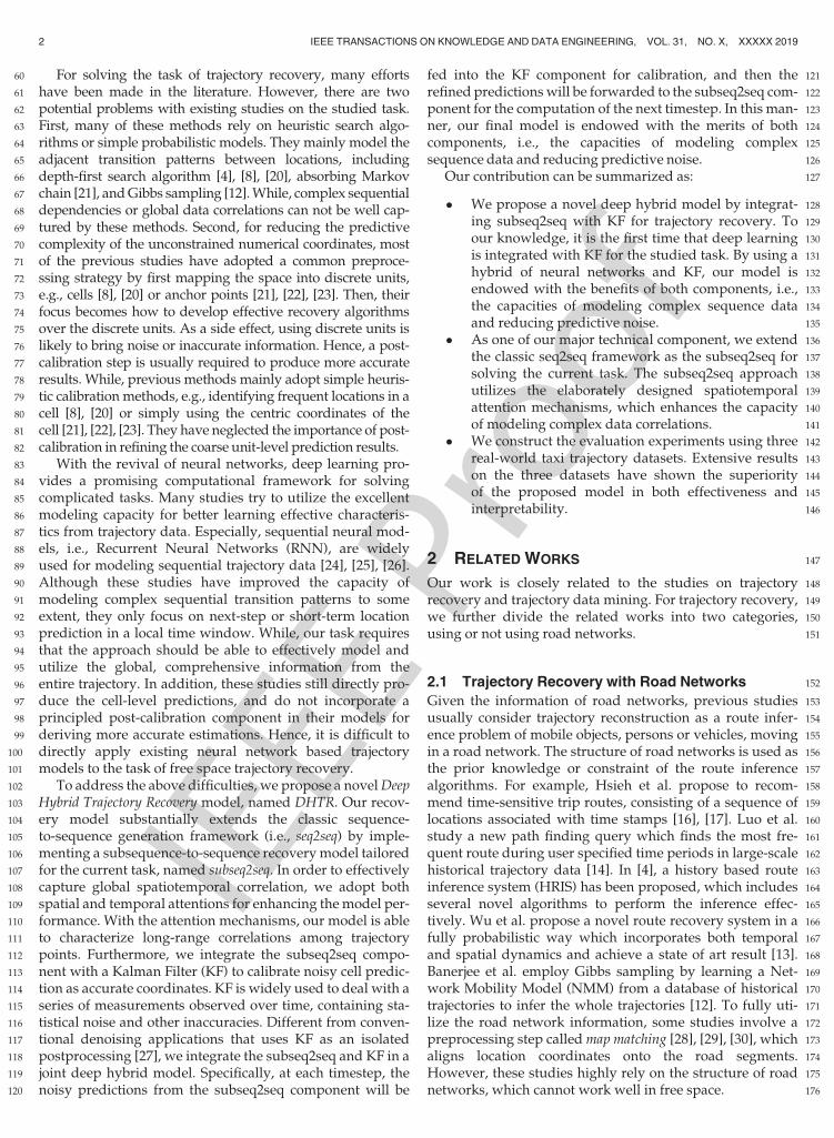
Fig. 3. The illustration for the integration of subseq2seq with Kalman Fil-ter. We can see there are three data flows in the model: i) The flow ofthe hidden state hhi in the subseq2seq component (highlighted by pink),which captures the long-range dependencies or correlations over thecell sequence. ii) The flow of gg;HH in the KF component (highlighted byblue), which calibrate coarse cell coordinates as fine-grained trajectorypoint coordinates. iii) The flow of the predicted cell coordinate zzi and itscalibrated coordinate zzi (including the middle variables NNi and ai,highlighted by green), which are passed between the KF componentand the subseq2seq component to integrate the two component as ahybrid model.

WANG ET AL.: DEEP TRAJECTORY RECOVERYWITH FINE-GRAINED CALIBRATION USING KALMAN FILTER 7

IEEE P

roof

L2 ¼ 1

2

Xð~t;tÞ2D

Xai2t and ai =2 ~t

�ai:x

ai:y

� �� zzi

�2

; (23)

679679

680 where zzi is the output of KF component at timestep i and

681ai:xai:y

� �is the actual coordinate vector for the ith point.

682 4.5 Model Learning

683 The final model loss consists of two parts, and we use a lin-684 ear combination way to integrate both loss functions

Ltotal ¼ L1 þ � � L2; (24)686686

687 where L1 and L2 are the loss functions defined in Eqs. (5)688 and (23) respectively, and � is a tuning parameter to balance689 the gradients of two loss functions in our work. Since our690 method is a hybrid model, it will be difficult to directly opti-691 mize the whole model. We adopt a separated approach to692 train the model parameters. Specifically, at each iteration,693 we first optimize the subseq2seq component and then694 update the KF component using the learned RNN695 parameters.696 For learning the subseq2seq component, it is relatively697 straightforward to optimize the L1 in Eq. (5). We apply the698 cross entropy as the loss function to train our subseq2seq699 model. Once we obtain the parameters for the subseq2seq700 component, we next optimize the KF component.701 While, the optimization of KF is more difficult. In the KF702 component, we have the following parameter matrices to703 learn, including MM, NN , FF, CC. Note that with our model, NN704 can be directly computed using the parameters from the705 subseq2seq component. The transformation matrices FF and706 CC are set as a priori based on general knowledge. Then, our707 focus is how to learn the state covariance matrixMM.708 Since the KF component is coupled with the subseq2seq,709 we can not directly use the traditional optimization algo-710 rithm, such as the discriminative training approach in [43],711 to infer the KF parameter of our model. Inspired by the712 learning methods of backprop Kalman filter proposed713 in [44], we propose an error Back Propagation Through Time714 for Kalman Filter algorithm, abbreviated to BPTT-KF, to715 optimize the parameter matrix MM of the KF component in716 our model.717 The gradients from timestep iþ l to the procedure718 covariance at timestep i can be derived as follows

@L�iþl

@MMi

¼ @L�iþl

@zziþl

@zziþl@ggiþljiþl

Yiþlk0¼iþ1

@ggk0 jk0@ggk0�1jk0�1

@ggiji@MMi

¼ ai:x

ai:y

� �� zziþl

� �CCiþl

Yiþlk0¼iþ1

ðII �KKk0CCk0 ÞFFk0@ggiji@MMi

;

720720

721 where L�i is the squared error between the real coordinates

722 and the predicted values, which is defined as

L�i ¼ 1

2

�ai:xai:y

� �� zzi

�2

: (25)724724

725

726For a trajectory with a length n, we can accumulate the727gradients of MMi from the current position to the end of the728trajectory as

@L2

@MMi¼

Xni0¼i

@L�i0

@MMi: (26)

730730

731Then the parameter MMi is optimized using the gradient732descent approach.

7335 EXPERIMENTS

734In this section, we first set up the experiments, and then735present the performance comparison and result analysis.

7365.1 Experimental Setup

7375.1.1 Construction of the Evaluation Set

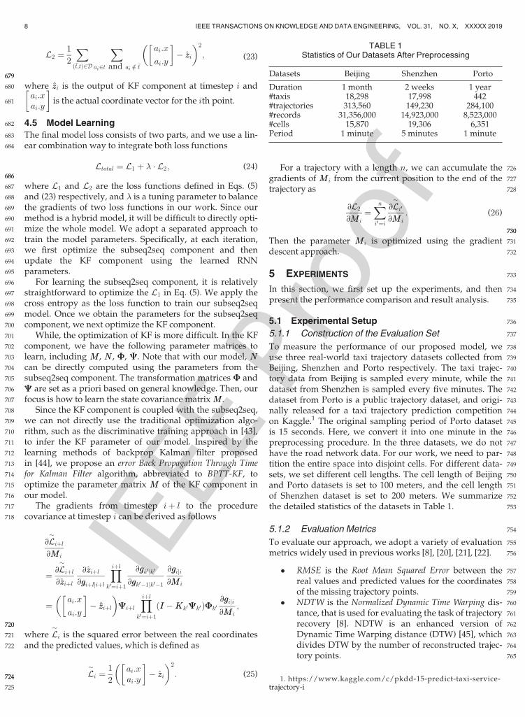
738To measure the performance of our proposed model, we739use three real-world taxi trajectory datasets collected from740Beijing, Shenzhen and Porto respectively. The taxi trajec-741tory data from Beijing is sampled every minute, while the742dataset from Shenzhen is sampled every five minutes. The743dataset from Porto is a public trajectory dataset, and origi-744nally released for a taxi trajectory prediction competition745on Kaggle.1 The original sampling period of Porto dataset746is 15 seconds. Here, we convert it into one minute in the747preprocessing procedure. In the three datasets, we do not748have the road network data. For our work, we need to par-749tition the entire space into disjoint cells. For different data-750sets, we set different cell lengths. The cell length of Beijing751and Porto datasets is set to 100 meters, and the cell length752of Shenzhen dataset is set to 200 meters. We summarize753the detailed statistics of the datasets in Table 1.

7545.1.2 Evaluation Metrics

755To evaluate our approach, we adopt a variety of evaluation756metrics widely used in previous works [8], [20], [21], [22].

757� RMSE is the Root Mean Squared Error between the758real values and predicted values for the coordinates759of the missing trajectory points.760� NDTW is the Normalized Dynamic Time Warping dis-761tance, that is used for evaluating the task of trajectory762recovery [8]. NDTW is an enhanced version of763Dynamic Time Warping distance (DTW) [45], which764divides DTW by the number of reconstructed trajec-765tory points.

TABLE 1Statistics of Our Datasets After Preprocessing

Datasets Beijing Shenzhen Porto

Duration 1 month 2 weeks 1 year#taxis 18,298 17,998 442#trajectories 313,560 149,230 284,100#records 31,356,000 14,923,000 8,523,000#cells 15,870 19,306 6,351Period 1 minute 5 minutes 1 minute

1. https://www.kaggle.com/c/pkdd-15-predict-taxi-service-trajectory-i

8 IEEE TRANSACTIONS ON KNOWLEDGE AND DATA ENGINEERING, VOL. 31, NO. X, XXXXX 2019

IEEE P

roof

766 � LCSS [46] is the measurement for the length of the Lon-767 gest Common Sub-Sequence between two target sequen-768 ces. It allows the skip trajectory points when necessary,769 which is helpful to reduce the influence of noises.770 � EDR [47] is the Edit Distance on Real sequence, which is771 also robust to noise and addresses some deficiencies772 in LCSS.773 Note that the original LCSS and EDR are intended to deal774 with sequences of discrete symbols. Here, we assume two775 continuous points are the same if their distance is smaller776 than a predefined threshold of 0.2 kilometers. For ease of anal-777 ysis, we subtracting the value of LCSS and EDR from one, so778 all the fourmetrics have the same tendency: smaller is better.

779 5.1.3 Task Setting

780 For each of the three datasets, we divide it into three parts781 with the splitting ratio of 7 : 1 : 2, namely training set, vali-782 dation set and test set. In our datasets, all the trajectories are783 completely sampled. Hence, we randomly generate the sub-784 trajectories using a sampling rate of r%. In other words, for785 each complete trajectory, we only keep r% of sampled tra-786 jectory points from it randomly. For the training set, we gen-787 erate random sub-trajectories at each iteration. While, for788 the test set, we generate and fix the sub-trajectories for pre-789 diction, and the complete trajectory are held out as ground-790 truth for evaluation. We further vary the sampling rate of791 r% in the set f30%; 50%; 70%g For reliable evaluation, we792 repeat the above process five times, and report the average793 results on the five evaluation sets.

794 5.1.4 Methods to Compare

795 We consider using the following successful methods for796 comparison:

797� RICK [8]: It builds a routable graph from uncertain798trajectories, and then answers a users online query (a799sequence of point locations) by searching top-k800routes on the graph.801� MPR [21]: It can discover the most popular route802from a transfer network based on the popularity803indicators in a breadth-first manner.804� DeepMove [26]: It is a multi-modal embedding recur-805rent neural network that can capture the complicated806sequential transitions by jointly embedding the mul-807tiple factors that govern the human mobility.808� STRNN [32]: It models local temporal and spatial809contexts in each layer with transition matrices for810different time intervals and geographical distances.811Among the four baselines, RICK and MPR are classic812search algorithms, while DeepMove and STRNN are newly-813proposed deep learning methods for next-step trajectory pre-814diction. To our knowledge, no deep learning methods are815directly applicable to trajectory recovery, and here we adapt816DeepMove and STRNN to this task by consecutively predict-817ing each missing point. In the trajectory recovery task, we fol-818low their original way to make the next-point prediction. To819recovery a missed point, we repeat the next-point prediction820several times according to the time interval until the cell of the821missed point is predicted. When the cell is predicted, we use822the centric location as the final prediction.823All the models have some parameters to tune. We either824follow the reported optimal parameter settings or optimize825each model separately using the validation set. For our826model, we adopt a two-layer LSTM network, the embed-827ding size of locations is set to 512. More detailed parameter828configuration can be found in Table 3. We will give the829detailed analysis on the parameter sensitivity of our model830in Section 5.3.3.

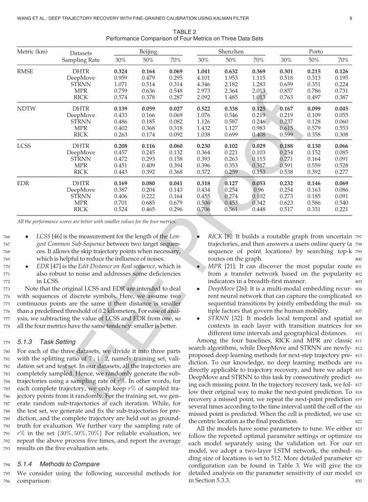
TABLE 2Performance Comparison of Four Metrics on Three Data Sets

Metric (km) Datasets Beijing Shenzhen Porto

Sampling Rate 30% 50% 70% 30% 50% 70% 30% 50% 70%

RMSE DHTR 0.324 0.164 0.069 1.041 0.632 0.369 0.301 0.215 0.126DeepMove 0.959 0.479 0.295 4.101 1.953 1.115 0.518 0.313 0.195STRNN 1.071 0.514 0.314 4.346 2.182 1.283 0.659 0.351 0.224MPR 0.759 0.636 0.548 2.973 2.364 2.013 0.857 0.786 0.731RICK 0.574 0.378 0.287 2.092 1.485 1.013 0.763 0.497 0.387

NDTW DHTR 0.139 0.059 0.027 0.522 0.338 0.125 0.167 0.099 0.045DeepMove 0.433 0.166 0.069 1.076 0.546 0.219 0.219 0.109 0.055STRNN 0.486 0.185 0.082 1.126 0.587 0.246 0.237 0.128 0.060MPR 0.402 0.368 0.318 1.432 1.127 0.983 0.615 0.579 0.553RICK 0.263 0.174 0.092 1.038 0.699 0.408 0.599 0.358 0.308

LCSS DHTR 0.208 0.116 0.060 0.230 0.102 0.029 0.188 0.130 0.066DeepMove 0.457 0.245 0.132 0.364 0.221 0.103 0.254 0.152 0.085STRNN 0.472 0.293 0.158 0.393 0.263 0.115 0.271 0.164 0.091MPR 0.451 0.409 0.394 0.396 0.353 0.317 0.591 0.559 0.528RICK 0.443 0.392 0.368 0.372 0.259 0.153 0.538 0.392 0.277

EDR DHTR 0.169 0.080 0.041 0.318 0.127 0.053 0.232 0.146 0.069DeepMove 0.387 0.204 0.143 0.434 0.254 0.96 0.254 0.163 0.086STRNN 0.406 0.222 0.164 0.455 0.274 0.102 0.273 0.185 0.091MPR 0.701 0.685 0.679 0.506 0.453 0.342 0.623 0.586 0.540RICK 0.524 0.465 0.296 0.706 0.561 0.448 0.517 0.331 0.221

All the performance scores are better with smaller values for the four metrics.

WANG ET AL.: DEEP TRAJECTORY RECOVERYWITH FINE-GRAINED CALIBRATION USING KALMAN FILTER 9

IEEE P

roof

831 5.2 Result and Analysis

832 The performance of all methods has been presented in833 Table 2. It can be observed that:

834 (1) Comparing the two traditional algorithms, we can835 see RICK is much better than MPR. RICK is based on836 the classic A* search algorithm, and MPR is based on837 the graph search algorithm. MPR involves much838 computation over the construction of the graph,839 which leads it is not suitable for large-scale data.840 (2) For the two neural network models, DeepMove is841 better than STRNN, since it incorporates more kinds842 of context information such as history information.843 Overall, DeepMove is better than the two traditional844 methods RICK and MPR. RICK is a competitive845 baseline, since it uses a series of heuristic refinement846 techniques for enhancing the prediction perfor-847 mance. As a comparison, DeepMove and STRNN848 mainly rely on the automatic learning of useful pat-849 terns or characteristics from original data.850 (3) Finally, our proposed model DHTR consistently out-851 perform all the baselines on three datasets with four852 metrics. Especially, the improvement ratios with a853 larger sampling rate is more significant. The underly-854 ing reasons for improvement lie in two aspects. First,855 we specially design a subseq2seq model equipped856 with the spatiotemporal attention for the task of tra-857 jectory recovery, which is able to fully utilize the spa-858 tiotemporal information in observed sub-trajectory.859 Second, we use the KF component to calibrate the860 coarse estimate by reducing prediction noise.

861 5.3 Detailed Analysis of Our Model

862 As shown in previous experiments, our model has achieved863 a significant improvement over all the baselines. In this864 part, we construct more detailed analysis of the proposed865 model for better understanding why it works well. Our866 model has two major technical contributions. First, we867 adopt the subseq2seq model for trajectory recovery, and868 incorporate the spatiotemporal attention mechanism to869 enhance the capacity of modeling complex dependencies or

870correlations for trajectory data. Second, we integrate the871subseq2seq model with the KF component, which further872uses a dynamic covariance for prediction. Next, we analyze873the effect of these two contributions, and then report the874results of parameter tuning.875For ease of analysis, we only report the average RMSE876performance on the Beijing dataset and Porto dataset, while877the results on the Shenzhen dataset using other metrics are878similar and omitted here.

8795.3.1 The Effect of the Spatiotemporal Attention

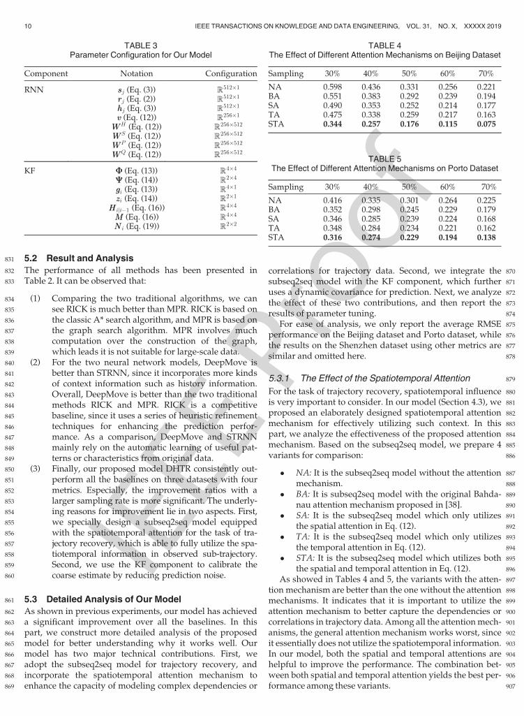
880For the task of trajectory recovery, spatiotemporal influence881is very important to consider. In our model (Section 4.3), we882proposed an elaborately designed spatiotemporal attention883mechanism for effectively utilizing such context. In this884part, we analyze the effectiveness of the proposed attention885mechanism. Based on the subseq2seq model, we prepare 4886variants for comparison:

887� NA: It is the subseq2seq model without the attention888mechanism.889� BA: It is subseq2seq model with the original Bahda-890nau attention mechanism proposed in [38].891� SA: It is the subseq2seq model which only utilizes892the spatial attention in Eq. (12).893� TA: It is the subseq2seq model which only utilizes894the temporal attention in Eq. (12).895� STA: It is the subseq2seq model which utilizes both896the spatial and temporal attention in Eq. (12).897As showed in Tables 4 and 5, the variants with the atten-898tion mechanism are better than the one without the attention899mechanisms. It indicates that it is important to utilize the900attention mechanism to better capture the dependencies or901correlations in trajectory data. Among all the attentionmech-902anisms, the general attention mechanism works worst, since903it essentially does not utilize the spatiotemporal information.904In our model, both the spatial and temporal attentions are905helpful to improve the performance. The combination bet-906ween both spatial and temporal attention yields the best per-907formance among these variants.

TABLE 3Parameter Configuration for Our Model

Component Notation Configuration

RNN ssj (Eq. (3)) R512�1rrj (Eq. (2)) R512�1hhj (Eq. (3)) R512�1vv (Eq. (12)) R256�1

WWH (Eq. (12)) R256�512WWS (Eq. (12)) R256�512WWP (Eq. (12)) R256�512WWQ (Eq. (12)) R256�512

KF FF (Eq. (13)) R4�4CC (Eq. (14)) R2�4ggi (Eq. (13)) R4�1zzi (Eq. (14)) R2�1

HHiji�1 (Eq. (16)) R4�4MM (Eq. (16)) R4�4NNi (Eq. (19)) R2�2

TABLE 4The Effect of Different Attention Mechanisms on Beijing Dataset

Sampling 30% 40% 50% 60% 70%

NA 0.598 0.436 0.331 0.256 0.221BA 0.551 0.383 0.292 0.239 0.194SA 0.490 0.353 0.252 0.214 0.177TA 0.475 0.338 0.259 0.217 0.163STA 0.344 0.257 0.176 0.115 0.075

TABLE 5The Effect of Different Attention Mechanisms on Porto Dataset

Sampling 30% 40% 50% 60% 70%

NA 0.416 0.335 0.301 0.264 0.225BA 0.352 0.298 0.245 0.229 0.179SA 0.346 0.285 0.239 0.224 0.168TA 0.348 0.284 0.234 0.221 0.162STA 0.316 0.274 0.229 0.194 0.138

10 IEEE TRANSACTIONS ON KNOWLEDGE AND DATA ENGINEERING, VOL. 31, NO. X, XXXXX 2019

IEEE P

roof

908 5.3.2 The Effect of the Kalman Filter Component

909 A key contribution of our model is the integration of the910 subseq2seq model with the KF component. In this section,911 we examine the effect of KF component on the model per-912 formance. Especially, in the standard KF, the covariance913 matrix NNi for the observation is static and all the timesteps914 share the same covariance matrix. In our model, we use the915 dynamic covariance matrices for modeling varying predic-916 tive uncertainty with time.917 Here, we prepare four variants of our model for compari-918 son. The first variant is the subseq2seq model (including the919 spatiotemporal attention) without the KF component. The920 second and third variants are the subseq2seq model inte-921 grated with the KF component using static and dynamic922 covariances respectively. While, the fourth variant is using923 the standard KF as a post-processing to filter the trajectory924 recovered by the subseq2seq model.925 For ease of comparison, we take the variant without KF926 as the reference, and compute the improvement ratios of the927 other three variants over it. We also consider the compari-928 sons with different sampling rates. We present the results in929 Tables 6 and 7. As we can see, the two variants integrating930 the KF component and the subseq2seq component as a931 whole are better than the one using KF as a post-processing.932 The dynamic covariance have better performance than the933 static covariance. Interestingly, with the increase of the sam-934 pling rate, the improvements become larger. It indicates935 that when we have more observed data, the estimation of936 KF can become more accurate and the calibration of KF937 component are more efficient.

938 5.3.3 Parameter Tuning

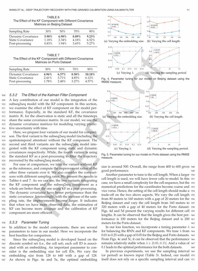
939 In addition to the model components, there are several940 parameters to tune in our model. Here we incorporate the941 best baseline for comparison.942 Since the subseq2seq model is developed based on the943 discrete symbol set (i.e., the cell set), each cell ID is associ-944 ated with an embedding. An important parameter to con-945 sider is the embedding size for cell IDs. We vary the946 embedding size from 128 to 640 with a gap of 128.947 As shown in Figs. 4a and 5a, the optimal embedding

948size is around 500. Overall, the range from 400 to 600 gives949good performance.950Another parameter to tune is the cell length. When a larger951cell length is used, we will have fewer cells to model. In this952case, we have a small complexity for the cell sequence, but the953numerical predictions for the coordinates become coarse and954vice versa. Hence, the setting of the cell length should make a955trade-off on the two above aspects. We vary the cell length956from 80 meters to 160 meters with a gap of 20 meters for the957Beijing dataset and vary the cell length from 160 meters to958320 meters with a gap of 40 meters for the Porto dataset.959Figs. 4d and 5d present the varying results for different cell960lengths. It can be observed that the length gives the best per-961formance is 100 meters for the Beijing dataset and is 200962meters for the Porto dataset.963In our loss function, we incorporate a tuning parameter �964for balancing the RNN and KF components. We tune � from9650.01 to 0.25with a gap of 0.05 for the Beijing and Porto datasets.966From Figs. 4c and 5c, it can be observed that the performance967remains relatively stable when � 2 ½0:05; 0:15�. And a value of9680.1 leads to the optimal performance for the both datasets.969In previous experiments, we use the sampling interval970(or period) as known input (Table 3). Indeed, our model971itself does not rely on a specific sampling interval and can

TABLE 6The Effect of the KF Component with Different Covariance

Matrices on Beijing Dataset

Sampling Rate 30% 50% 70% 90%

Dynamic Covariance 5.90% 6.98% 8.09% 9.23%Static Covariance 1.18% 2.34% 4.18% 6.52%Post-processing 0.83% 1.94% 3.65% 5.27%

TABLE 7The Effect of the KF Component with Different Covariance

Matrices on Porto Dataset

Sampling Rate 30% 50% 70% 90%

Dynamic Covariance 4.96% 6.37% 8.58% 10.18%Static Covariance 2.41% 3.71% 4.85% 6.12%Post-processing 1.78% 2.48% 3.27% 4.57%

Fig. 4. Parameter tuning for our model on Beijing dataset using theRMSE measure.

Fig. 5. Parameter tuning for our model on Porto dataset using the RMSEmeasure.

WANG ET AL.: DEEP TRAJECTORY RECOVERYWITH FINE-GRAINED CALIBRATION USING KALMAN FILTER 11

IEEE P

roof

972 work with different sampling periods. To see this, we vary973 the sampling period in the set f1; 3; 5; 10; 15g. Figs. 4d and974 5d present the results with different sampling periods for975 the Beijing and Porto datasets. Overall, a larger sampling976 period will yield a worse performance, since the input has977 contained fewer known points.

978 5.4 Qualitative Analysis on the Model979 Interpretability

980 Another major benefit of our model is that the intermediate981 results for predictions are highly interpretable. In this sec-982 tion, we present some qualitative analysis by visualizing the983 attention weights and the covariance matrices.

984 5.4.1 Visualizing Attention Weights of the Subseq2seq

985 Model

986 We first present a qualitative example for understanding the987 attention weights in our model. We take a trajectory988 sequence from the Beijing dataset. The complete sequence989 consists of 100 trajectory points sampled by minute. After990 removing the points for predictions, we keep 30 random991 points as the observed sub-trajectory. The task is to recon-992 struct the missing 70 points in the original trajectory. Fig. 6a993 gives the overview of the trajectory sequence, where the994 observed points are marked as purple.995 Fig. 6b presents the comparison between our proposed996 spatiotemporal attention mechanism and the Bahdanau997 attention mechanism in [38]. In the experiment, we respec-998 tively use the Bahdanau attention and the spatiotemporal999 attention in our model to recovery the missing trajectory

1000 points. The attention weights of the two type of attentions1001 are plotted in Fig. 6b. As shown in the figure, there are two1002 matrices with the size of 30� 100. The upper is for the Bah-1003 danau attention, and the lower is for our spatiotemporal1004 attention. The horizontal axes of the matrices express the1005 100 trajectory points of the complete sequence, and the ver-1006 tical axes express the 30 random points. The cells of the Bah-1007 danau attention matrix denote ui;j that are calculated by1008 Eq. (9), and of the spatiotemporal attention denote ui;j that

1009are calculated for Eq. (12). The values of the matrix cells are1010the darker the higher.1011As shown in the figure, the Bahdanau attention does not1012consider the spatiotemporal information for modeling trajec-1013tory data, and it produces dispersive attention weights over1014the observed points. As a comparison, our proposed method1015generates a skew, focused distribution of attention weights.1016With our attention mechanism, a trajectory point to be pre-1017dicted is mainly influenced by the nearby sampled points.1018Hence, our attention mechanism is more capable of modeling1019the spatiotemporal characteristics of trajectory data.

10205.4.2 Visualizing the Dynamic Covariance of Kalman

1021Filter

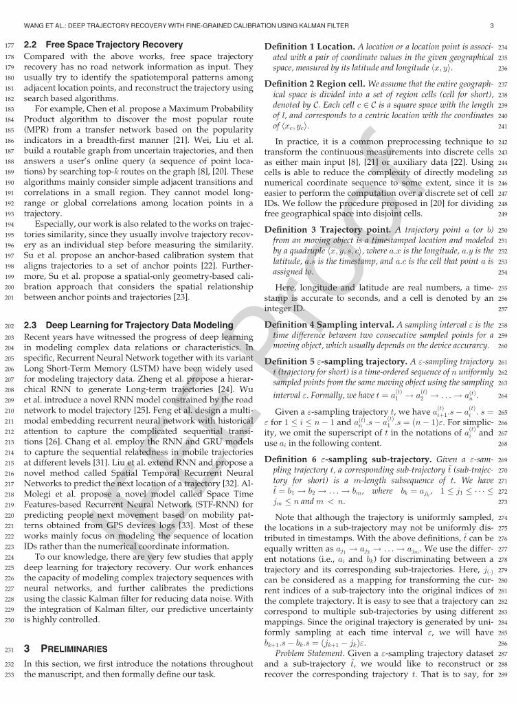
1022In our model, we model the dynamic covariance for the pre-1023dictions with time, and trace the varying of the predictive1024uncertainty for the estimations. Therefore, besides the esti-1025mated results, both the subseq2seq component and the KF1026component are able to give confidence distribution over the1027predictions.1028Fig. 7 illustrates an example of how prediction uncertainty1029in our model changes with time. In this example, we present1030three trajectory points from a trajectory sequence, namely1031ai�2, ai�1 and ai. The prediction uncertainty of the these points1032are plotted on the figure as heat map. A darker color indicates1033a more confident prediction. At timestamp i, we give a detail1034of the prediction uncertainty for different components of our1035model. Here, the subseq2seq model outputs a noisy predic-1036tionwith a confidence distribution labeled as “Predicted by sub-1037seq2seq at i”. The noisy prediction is subsequently fed into the1038KF component. Recall that the KF component involves two1039steps. In the prediction step, KF makes a state prediction with1040a confidence distribution labeled as “Predicted by KF at i”,1041which pulls the prediction towards the target point. Then,1042after the update step, our model given a final prediction with1043a confidence distribution labeled as “Calibrated by KF at i”,1044which ismore close to the target point.1045Different from previous deep learning models for trajec-1046tory data, our model is able to explicitly characterize the

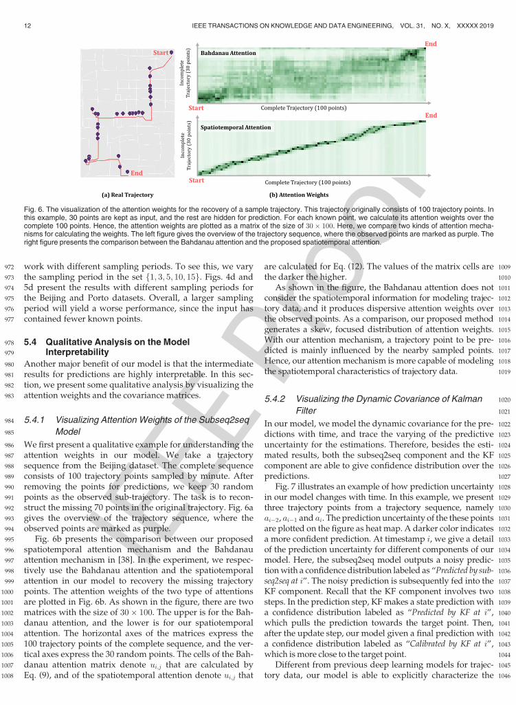
Fig. 6. The visualization of the attention weights for the recovery of a sample trajectory. This trajectory originally consists of 100 trajectory points. Inthis example, 30 points are kept as input, and the rest are hidden for prediction. For each known point, we calculate its attention weights over thecomplete 100 points. Hence, the attention weights are plotted as a matrix of the size of 30� 100. Here, we compare two kinds of attention mecha-nisms for calculating the weights. The left figure gives the overview of the trajectory sequence, where the observed points are marked as purple. Theright figure presents the comparison between the Bahdanau attention and the proposed spatiotemporal attention.

12 IEEE TRANSACTIONS ON KNOWLEDGE AND DATA ENGINEERING, VOL. 31, NO. X, XXXXX 2019

IEEE P

roof1047 predictive uncertainty (e.g., the heat map in Fig. 7). It is use-

1048 ful to understand the internal working mechanism of the1049 prediction model.

1050 6 CONCLUSIONS

1051 In this paper, we proposed a novel deep hybrid model for1052 trajectory recovery in free space. Our model integrated the1053 subseq2seq component with the KF component. It was1054 endowed with the merits of both components, i.e., the1055 capacities of modeling complex sequence data and reducing1056 predictive noise. We constructed three large trajectory data-1057 sets for evaluation. The experimental results have shown1058 that our model is superior to previous methods in the task1059 of trajectory recovery.1060 Currently, we test the proposed model with three taxi1061 trajectory datasets. We will consider applying our model to1062 trajectory data in more domains, e.g., animal trace. In our1063 work, we mainly focus the spatiotemporal correlations1064 among trajectory points. As future work, we will extend the1065 proposed model by incorporate more kinds of context infor-1066 mation, e.g., POI labels and user profiles.

1067 ACKNOWLEDGMENTS

1068 The work was supported by the National Natural Science1069 Foundation of China (Grant No. 61572059, 61872369,1070 71531001), and the Fundamental Research Funds for the1071 Central Universities. Dr.Wang’s workwas partially supported1072 by the National Key Research and Development Program of1073 China (Grant No. 2017YFC0820405) and the Science and Tech-1074 nology Project of Beijing (Grant No. Z.181100003518001).1075 Dr. Zhao’s work was partially supported by the Research1076 Funds of Renmin University of China (Grant No. 18XNLG22).1077 Dr. Feng’sworkwas partially supported by theOpenResearch1078 Program of Shenzhen Key Laboratory of Spatial Smart Sensing1079 and Services (ShenzhenUniversity).

1080 REFERENCES

1081 [1] W. X. Zhao, N. Zhou, A. Sun, J. R. Wen, J. Han, and E. Y. Chang, “A1082 time-aware trajectory embedding model for next-location recom-1083 mendation,”Knowl. Inf. Syst., vol. 56, no. 3, pp. 559–579, Sep. 2018.1084 [2] J. Wang, J. Wu, Z. Wang, F. Gao, and Z. Xiong, “Understanding1085 urban dynamics via context-aware tensor factorization with1086 neighboring regularization,” IEEE Trans. Knowl. Data Eng., early1087 access, May 7, 2019, doi: 10.1109/TKDE.2019.2915231.1088 [3] J. Yuan, Y. Zheng, X. Xie, and G. Sun, “T-drive: Enhancing driving1089 directions with taxi drivers’ intelligence,” IEEE Trans. Knowl. Data1090 Eng., vol. 25, no. 1, pp. 220–232, Jan. 2013.

1091[4] K. Zheng, Y. Zheng, X. Xie, and X. Zhou, “Reducing uncertainty of1092low-sampling-rate trajectories,” in Proc. IEEE 28th Int. Conf. Data1093Eng., 2012, pp. 1144–1155.1094[5] M. Ulm and N. Brandie, “Robust online trajectory clustering with-1095out computing trajectory distances,” in Proc. IEEE 21st Int. Conf.1096Pattern Recognit., 2012, pp. 2270–2273.1097[6] D. Pfoser, C. S. Jensen, and Y. Theodoridis, “Novel approaches in1098query processing for moving object trajectories,” in Proc. ACM109926th Int. Conf. Very Large Data Bases, 2000, pp. 395–406.1100[7] Y. Zheng, L. Liu, L. Wang, and X. Xie, “Learning transportation1101mode from raw GPS data for geographic applications on the1102web,” in Proc. ACM 16th Conf. World Wide Web, 2008, pp. 247–256.1103[8] L. Y. Wei, Y. Zheng, and W. C. Peng, “Constructing popular1104routes from uncertain trajectories,” in Proc. ACM 18th SIGKDD1105Int. Conf. Knowl. Discovery Data Mining, 2012, pp. 195–203.1106[9] Y. Zheng, “Trajectory data mining: An overview,” ACM Trans.1107Intell. Syst. Technol., vol. 6, no. 3, 2015, Art. no. 29.1108[10] S. Guo, C. Chen, J. Wang, Y. Liu, K. Xu, Z. Yu, D. Zhang, and1109D. M. Chiu, “Rod-revenue: Seeking strategies analysis and reve-1110nue prediction in ride-on-demand service using multi-source1111urban data,” IEEE Trans. Mobile Comput., early access, Jun. 10,11122019, doi: 10.1109/TMC.2019.2921959.1113[11] B. Liao, J. Zhang, C. Wu, D. McIlwraith, T. Chen, S. Yang, Y. Guo,1114and F. Wu, “Deep sequence learning with auxiliary information1115for traffic prediction,” in Proc. 24th ACM SIGKDD Int. Conf. Knowl.1116Discovery Data Mining, 2018, pp. 537–546.1117[12] P. Banerjee, S. Ranu, and S. Raghavan, “Inferring uncertain trajec-1118tories from partial observations,” in Proc. IEEE 14th Int. Conf. Data1119Mining, 2014, pp. 30–39.1120[13] H. Wu, J. Mao, W. Sun, B. Zheng, H. Zhang, Z. Chen, and1121W. Wang, “Probabilistic robust route recovery with spatio-tempo-1122ral dynamics,” in Proc. ACM 22nd SIGKDD Int. Conf. Knowl. Dis-1123covery Data Mining, 2016, pp. 1915–1924.1124[14] W. Luo, H. Tan, L. Chen, and L. M. Ni, “Finding time period-1125based most frequent path in big trajectory data,” in Proc. ACM112632th SIGMOD Int. Conf. Manage. Data, 2013, pp. 713–724.1127[15] H. Liang and K. Wang, “Constructing top-k routes with personal-1128ized submodular maximization of POI features,” CoRR, vol. abs/11291710.03852, 2017. [Online]. Available: http://arxiv.org/abs/11301710.038521131[16] H. P. Hsieh, C. T. Li, and S. D. Lin, “Exploiting large-scale check-1132in data to recommend time-sensitive routes,” in Proc. 18th ACM1133SIGKDD Int. Conf. Knowl. Discovery Data Mining, 2012, pp. 55–62.1134[17] H. Hsieh, C. Li, and S. Lin, “Measuring and recommending time-1135sensitive routes from location-based data,” in Proc. 38th Int. ACM1136SIGIR Conf. Res. Develop. Inf. Retrieval, 2015, pp. 4193–4196.1137[18] F. Xu, Z. Tu, Y. Li, P. Zhang, X. Fu, and D. Jin, “Trajectory recov-1138ery from ash: User privacy is not preserved in aggregated mobility1139data,” in Proc. 26th Int. Conf. World Wide Web, 2017, pp. 1241–1250.1140[Online]. Available: https://doi.org/10.1145/3038912.30526201141[19] K. Ouyang, R. Shokri, D. S. Rosenblum, and W. Yang, “A non-1142parametric generative model for human trajectories,” in Proc. 27th1143Int. Joint Conf. Artif. Intell., Jul. 2018, pp. 3812–3817. [Online].1144Available: https://doi.org/10.24963/ijcai.2018/5301145[20] H. Liu, L.-Y. Wei, Y. Zheng, M. Schneider, andW.-C. Peng, “Route1146discovery from mining uncertain trajectories,” in Proc. IEEE 11th1147Int. Conf. Data Mining Workshops, 2011, pp. 1239–1242.1148[21] Z. Chen, H. T. Shen, and X. Zhou, “Discovering popular routes1149from trajectories,” in Proc. IEEE 27th Int. Conf. Data Eng., 2011,1150pp. 900–911.

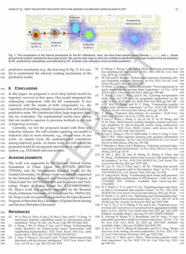
Fig. 7. The visualization of the internal procedures for the KF calibrations. Here, we have three sample points, namely ai�2, ai�1 and ai, whoseground-truth location indicated by the purple points. We use the heat maps to show the confidence distribution of sample locations that are predictedby KF, predicted by subseq2seq, and calibrated by KF. A darker color indicates a more confident prediction.

WANG ET AL.: DEEP TRAJECTORY RECOVERYWITH FINE-GRAINED CALIBRATION USING KALMAN FILTER 13

IEEE P

roof

1151 [22] H. Su, K. Zheng, H. Wang, J. Huang, and X. Zhou, “Calibrating1152 trajectory data for similarity-based analysis,” in Proc. ACM 32th1153 SIGMOD Int. Conf. Manage. Data, 2013, pp. 833–844.1154 [23] H. Su, K. Zheng, J. Huang, H. Wang, and X. Zhou, “Calibrating1155 trajectory data for spatio-temporal similarity analysis,” Int. J. Very1156 Large Data Bases, vol. 24, no. 1, pp. 93–116, 2015.1157 [24] S. Zheng, Y. Yue, and P. Lucey, “Generating long-term trajectories1158 using deep hierarchical networks,” in Proc. 31st Int. Conf. Neural1159 Inf. Process. Syst., 2017, pp. 1543–1551.1160 [25] H. Wu, Z. Chen, W. Sun, B. Zheng, and W. Wang, “Modeling tra-1161 jectories with recurrent neural networks,” in Proc. 26th Int. Joint1162 Conf. Artif. Intell., 2017, pp. 3083–3090.1163 [26] J. Feng, Y. Li, C. Zhang, F. Sun, F. Meng, A. Guo, and D. Jin,1164 “DeepMove: Predicting human mobility with attentional recur-1165 rent networks,” in Proc. ACM 26th Conf. World Wide Web, 2018,1166 pp. 1459–1468.1167 [27] R. G. Brown, P. Y. Hwang, et al., Introduction to Random Signals and1168 Applied Kalman Filtering, vol. 3. New York, NY, USA: Wiley, 1992.1169 [28] O. Pink and B. Hummel, “A statistical approach to map matching1170 using road network geometry, topology and vehicular motion1171 constraints,” in Proc. IEEE 11th Int. Conf. Intell. Transp. Syst., 2008,1172 pp. 862–867.1173 [29] Y. Lou, C. Zhang, Y. Zheng, X. Xie, W. Wang, and Y. Huang,1174 “Map-matching for low-sampling-rate GPS trajectories,” in Proc.1175 ACM 17th SIGSPATIAL Int. Conf. Advances Geographic Inf. Syst.,1176 2009, pp. 352–361.1177 [30] J. Yuan, Y. Zheng, C. Zhang, X. Xie, and G.-Z. Sun, “An interac-1178 tive-voting based map matching algorithm,” in Proc. IEEE 11th1179 Int. Conf. Mobile Data Manage., 2010, pp. 43–52.1180 [31] C. Yang, M. Sun, W. X. Zhao, Z. Liu, and E. Y. Chang, “A neural1181 network approach to jointly modeling social networks and mobile1182 trajectories,” ACM Trans. Inf. Syst., vol. 35, no. 4, pp. 36:1–36:28,1183 2017.1184 [32] Q. Liu, S. Wu, L. Wang, and T. Tan, “Predicting the next location:1185 A recurrent model with spatial and temporal contexts,” in Proc.1186 30th AAAI Conf. Artif. Intell., 2016, pp. 194–200.1187 [33] A. Al-Molegi, M. Jabreel, and B. Ghaleb, “STF-RNN: Space time1188 features-based recurrent neural network for predicting people1189 next location,” in Proc. IEEE Symp. Series Comput. Intell., 2016,1190 pp. 1–7.1191 [34] I. Sutskever, O. Vinyals, and Q. V. Le, “Sequence to sequence1192 learning with neural networks,” Proc. 28th Int. Conf. Neural Inf.1193 Process. Syst., 2014, pp. 3104–3112.1194 [35] S. Hochreiter and J. Schmidhuber, “Long short-term memory,”1195 Neural Comput., vol. 9, no. 8, pp. 1735–1780, 1997.1196 [36] M. Schuster and K. K. Paliwal, Bidirectional Recurrent Neural Net-1197 works. Piscataway, NJ, USA: IEEE Press, 1997.1198 [37] J. Gu, Z. Lu, H. Li, and V. O. K. Li, “Incorporating copying mecha-1199 nism in sequence-to-sequence learning,” in Proc. 54th Annu.1200 Meeting Assoc. Comput. Linguistics ACL’16, 2016, pp. 1631–1640.1201 [38] Y. Bengio and Y. LeCun, “Neural machine translation by jointly1202 learning to align and translate,” in Proc. 3rd Int. Conf. Learn. Repre-1203 sentations, 2015, pp. 1–15.1204 [39] A. Vaswani, N. Shazeer, N. Parmar, J. Uszkoreit, L. Jones,1205 A. N. Gomez, L. U. Kaiser, and I. Polosukhin, “Attention is all you1206 need,” in Proc. 31st Int. Conf. Neural Inf. Process. Syst., 2017,1207 pp. 6000–6010.1208 [40] J. Gehring, M. Auli, D. Grangier, D. Yarats, and Y. N. Dauphin,1209 “Convolutional sequence to sequence learning,” in Proc. 35th Int.1210 Conf. Mach. Learn., 2017, pp. 1243–1252.1211 [41] Q. Chen, Q. Hu, J. X. Huang, L. He, and W. An, “Enhancing recur-1212 rent neural networks with positional attention for question1213 answering,” in Proc. 40th Int. ACM SIGIR Conf. Res. Develop. Inf.1214 Retrieval, 2017, pp. 993–996.1215 [42] R. E. Kalman, “A new approach to linear filtering and prediction1216 problems,” J. Basic Eng. Trans., vol. 82, pp. 35–45, 1960.1217 [43] P. Abbeel, A. Coates, M. Montemerlo, A. Y. Ng, and S. Thrun,1218 “Discriminative training of kalman filters,” in Proc. Robot.: Sci.1219 Syst. I, 2005, pp. 289–296.1220 [44] T. Haarnoja, A. Ajay, S. Levine, and P. Abbeel, “Backprop KF:1221 Learning discriminative deterministic state estimators,” in Proc.1222 30th Int. Conf. Neural Inf. Process. Syst., 2016, pp. 4376–4384.1223 [45] J. B. Kruskal, “An overview of sequence comparison: Time warps,1224 string edits, and macromolecules,” Int. J. Mach. Tools Manufacture,1225 vol. 25, no. 2, pp. 201–237, 1983.1226 [46] J. K. Kearney and S. Hansen, “Stream editing for animation,” The1227 University of Iowa, Iowa City, IA, Rep. no. ADA231316, 1990.

1228[47] L. Chen and V. Oria, “Robust and fast similarity search for mov-1229ing object trajectories,” in Proc. ACM 24th SIGMOD Int. Conf. Man-1230age. Data, 2005, pp. 491–502.

1231Jingyuan Wang received the PhD degree from1232the Department of Computer Science and Tech-1233nology, Tsinghua University, Beijing, China. He is1234currently an associate professor of the School of1235Computer Science and Engineering, Beihang1236University, Beijing, China. He is also the head of1237the Beihang Interest Group on SmartCity1238(BIGSCity), and vice director of the Beijing City1239Lab (BCL). He published more than 30 papers on1240top journals and conferences, as well as named1241inventor on several granted US patents. His gen-1242eral area of research is data mining and machine1243learning, with special interests in smart cities.

1244Ning Wu received the BEng degree in computer1245science from Beihang University, China, in 2018.1246He is currently working toward the master’s1247degree in the School of Computer Science and1248Engineering, Beihang University. His research1249mainly focuses on urban data analysis.

1250Xinxi Lu received the PhD degree from the1251School of Electronic and Information Engineer-1252ing, Beihang University, Beijing, China. He is1253currently an associate professor of the School of1254Software, Beihang University, Beijing, China. He1255has engaged in information technology for more1256than 10 years, mainly focusing on cloud comput-1257ing, exploration and research in big data. He1258developed dozens of software applications, pub-1259lished more than 10 books and papers, as well as1260named inventor on several granted patents.

1261Wayne Xin Zhao received the PhD degree from1262Peking University, in 2014. He is currently an1263associate professor with the School of Informa-1264tion, Renmin University of China. His research1265interests are social data mining and recom-1266mender systems. He has published more than 601267referred papers in international conferences and1268journals. He is a member of the IEEE and ACM.

1269Kai Feng received the BEng degree in computer1270science from Beihang University, China, in 2018.1271He is currently working toward the master’s1272degree in the School of Computer Science and1273Engineering, Beihang University. His research1274mainly focuses on time series analysis.

1275" For more information on this or any other computing topic,1276please visit our Digital Library at www.computer.org/publications/dlib.

14 IEEE TRANSACTIONS ON KNOWLEDGE AND DATA ENGINEERING, VOL. 31, NO. X, XXXXX 2019