1

Definition, diagnosis, and origin of extremeweather and climate events

DAVID B. STEPHENSON

Condensed summary

Extreme weather and climate events are a major source of risk for all human

societies. There is a pressing need for more research on such events. Various

societal changes, such as increased populations in coastal and urban areas

and increasingly complex infrastructure, have made us potentially more vul-

nerable to such events than we were in the past. In addition, the properties

of extreme weather and climate events are likely to change in the twenty-first

century owing to anthropogenic climate change.

The definition, classification, and diagnosis of extreme events are far from

simple. There is no universal unique definition of what is an extreme event.

This chapter discusses these issues and presents a simple framework for

understanding extreme events that will help enable future work in this impor-

tant area of climate science and global reinsurance.

1.1 Introduction

Human society is particularly vulnerable to severe weather and climate events

that cause damage to property and infrastructure, injury, and even loss of life.

Although generally rare at any particular location, such events cause a dis-

proportionate amount of loss.

In this chapter, I attempt to describe a framework for classifying, diag-

nosing, and understanding extreme weather and climate events. The multi-

dimensional aspect of complex extreme events will be discussed, and

statistical methods will be presented for understanding simple extreme

events. Some preliminary ideas about the origin of extreme events will also

be presented.

Climate Extremes and Society, ed. H.F. Diaz and R. J. Murnane. Published by Cambridge UniversityPress. # Cambridge University Press 2008.

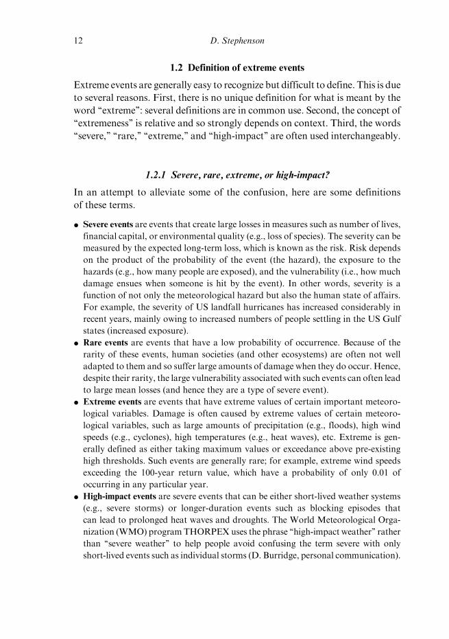
1.2 Definition of extreme events

Extreme events are generally easy to recognize but difficult to define. This is due

to several reasons. First, there is no unique definition for what is meant by the

word ‘‘extreme’’: several definitions are in common use. Second, the concept of

‘‘extremeness’’ is relative and so strongly depends on context. Third, the words

‘‘severe,’’ ‘‘rare,’’ ‘‘extreme,’’ and ‘‘high-impact’’ are often used interchangeably.

1.2.1 Severe, rare, extreme, or high-impact?

In an attempt to alleviate some of the confusion, here are some definitions

of these terms.

* Severe events are events that create large losses in measures such as number of lives,

financial capital, or environmental quality (e.g., loss of species). The severity can be

measured by the expected long-term loss, which is known as the risk. Risk depends

on the product of the probability of the event (the hazard), the exposure to the

hazards (e.g., how many people are exposed), and the vulnerability (i.e., how much

damage ensues when someone is hit by the event). In other words, severity is a

function of not only the meteorological hazard but also the human state of affairs.

For example, the severity of US landfall hurricanes has increased considerably in

recent years, mainly owing to increased numbers of people settling in the US Gulf

states (increased exposure).

* Rare events are events that have a low probability of occurrence. Because of the

rarity of these events, human societies (and other ecosystems) are often not well

adapted to them and so suffer large amounts of damage when they do occur. Hence,

despite their rarity, the large vulnerability associated with such events can often lead

to large mean losses (and hence they are a type of severe event).

* Extreme events are events that have extreme values of certain important meteoro-

logical variables. Damage is often caused by extreme values of certain meteoro-

logical variables, such as large amounts of precipitation (e.g., floods), high wind

speeds (e.g., cyclones), high temperatures (e.g., heat waves), etc. Extreme is gen-

erally defined as either taking maximum values or exceedance above pre-existing

high thresholds. Such events are generally rare; for example, extreme wind speeds

exceeding the 100-year return value, which have a probability of only 0.01 of

occurring in any particular year.

* High-impact events are severe events that can be either short-lived weather systems

(e.g., severe storms) or longer-duration events such as blocking episodes that

can lead to prolonged heat waves and droughts. The World Meteorological Orga-

nization (WMO) programTHORPEX uses the phrase ‘‘high-impact weather’’ rather

than ‘‘severe weather’’ to help people avoid confusing the term severe with only

short-lived events such as individual storms (D. Burridge, personal communication).

12 D. Stephenson

1.2.2 Multidimensional nature of extreme events

In addition to this potential source of confusion, extreme events have a

variety of different attributes and so cannot be completely described by a

single number. The multidimensional nature of extreme events is often over-

looked in rankings of the events based on only one of the attributes (e.g., the

category numbers for hurricanes based solely on maximum surface wind

speed).

Extreme events have attributes such as:

* rate (probability per unit time) of occurrence

* magnitude (intensity)

* temporal duration and timing

* spatial scale (footprint)

* multivariate dependencies

For example, a major hurricane is rare, has large-magnitude surface wind

speeds, has a generally large spatial scale (with the exception of certain small-

spatial-footprint events such as Hurricane Camille in 1969), and develops over

synoptic timescales ranging from hours to several days. In addition, the

severity of such events can also depend on the combination of extreme beha-

vior in more than one variable; for example, much hurricane damage is due

to extreme precipitation as well as extreme wind speeds. For example, a severe

ice storm can involve conditions for all three variables: temperature, wind,

and precipitation amount. The Intergovernmental Panel on Climate Change

(IPCC, 2001) defines ‘‘complex extreme’’ events as ‘‘severe weather associated

with particular climatic phenomena, often requiring a critical combination of

variables.’’ The magnitude of the losses depends on several meteorological

variables and hence dependencies between them.

The temporal duration of extreme events plays an important role in the

exposure and hence total losses. For example, the long duration of the flood-

ing in New Orleans caused by Hurricane Katrina led to large insurance losses

due to business interruption in addition to property damage losses. Temporal

duration also provides a useful way of classifying extreme events. The duration

is implicit when one describes an event as a ‘‘climate’’ extreme event rather than

a ‘‘weather’’ extreme event. The medical illness concepts of chronic and acute

can be usefully applied to weather and climate events:

* Acute extremes: events that have a rapid onset and follow a short but severe course.

Examples are short-lived weather systems such as tropical and extratropical

cyclones, polar lows, and convective storms with extreme values of meteorological

variables such as wind speed and precipitation that can lead to devastating wind,

Definition and origin of extreme events 13

flood, and ice damage. In addition to these obvious examples of high-impact

extreme events, there are less obvious acute extreme events, such as fog that causes

major transport disruption (e.g., at airports).

* Chronic extremes: events that last for a long period of time (e.g., longer than 3

months) or are marked by frequent recurrence. Examples are heat waves and

droughts that can lead to such impacts as critical water shortages, crop failure,

heat-related illness and mortality, and agricultural failure. Because of their

extended duration and generally lower intensity, chronic extreme events can often

be harder to define than acute extreme events, but they have the advantage that

there is more time to issue warnings and take protective actions. Note that not all

high-impact weather events are acute; for example, blocking weather events that

last several days are chronic events.

1.2.3 A simple taxonomy

One approach towards creating a definition is to try to list and classify all

events that one considers to be extreme. For example, the following events are

often cited as examples of extreme weather/climate events.

* Tropical cyclones and hurricanes (e.g., Typhoon Tracy, Hurricane Hugo, etc.).

These storms are the major source of global insured catastrophe loss after

earthquakes.

* Extratropical cyclones (e.g., the ‘‘Perfect Storm’’ that hit the northeast coast of

the United States, October 28–30, 1991). These storms are generally referred to as

‘‘windstorms’’ by the reinsurance industry.

* Convective phenomena such as tornadoes, waterspouts, and severe thunderstorms.

These phenomena can lead to extreme local wind speeds and precipitation

amounts on horizontal scales of up to about 10 km. Deep convection often leads

to precipitation in the form of hail, which can be very damaging to crops, cars, and

property.

* Mesoscale phenomena such as polar lows, mesoscale convective systems, and sting

jets. These features can lead to extreme wind speeds and precipitation amounts on

horizontal scales from 100 to 1,000 km.

* Floods of rivers, lakes, coasts, etc., due to severe weather conditions; for example,

river floods caused by intense precipitation over a short period (e.g., flash floods)

and persistent/recurrent precipitation over many days (e.g., wintertime floods

in northern Europe), river floods caused by rapid snowmelt due to a sudden

warm spell, or coastal floods caused by high sea levels due to wind-related storm

surges.

* Drought. Meteorological drought is defined usually on the basis of the degree of

dryness (in comparison to some ‘‘normal’’ or average amount) and the duration of

the dry period. Simple definitions relate actual precipitation departures to average

amounts on monthly, seasonal, or annual timescales. However, meteorological

14 D. Stephenson

drought also depends on other quantities such as evaporation that depend on

variables such as temperature.

* Heat waves. Periods of exceptionally warm temperatures can have profound

impacts on human health and agriculture. Duration is a key component determin-

ing the impact.

* Cold waves/spells (e.g., extremely cold days or a succession of frost days with

minimum temperatures below 0 8C).* Fog. Extremely low visibility has major impacts on various sectors such as aviation

and road transport.

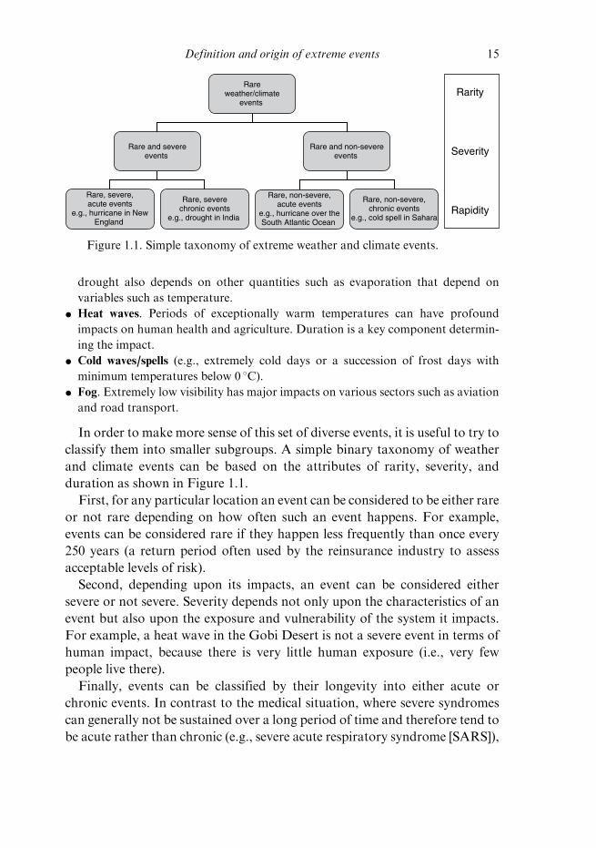
In order to make more sense of this set of diverse events, it is useful to try to

classify them into smaller subgroups. A simple binary taxonomy of weather

and climate events can be based on the attributes of rarity, severity, and

duration as shown in Figure 1.1.

First, for any particular location an event can be considered to be either rare

or not rare depending on how often such an event happens. For example,

events can be considered rare if they happen less frequently than once every

250 years (a return period often used by the reinsurance industry to assess

acceptable levels of risk).

Second, depending upon its impacts, an event can be considered either

severe or not severe. Severity depends not only upon the characteristics of an

event but also upon the exposure and vulnerability of the system it impacts.

For example, a heat wave in the Gobi Desert is not a severe event in terms of

human impact, because there is very little human exposure (i.e., very few

people live there).

Finally, events can be classified by their longevity into either acute or

chronic events. In contrast to the medical situation, where severe syndromes

can generally not be sustained over a long period of time and therefore tend to

be acute rather than chronic (e.g., severe acute respiratory syndrome [SARS]),

Rare, non-severe,acute events

e.g., hurricane over theSouth Atlantic Ocean

Rare, non-severe,chronic events

e.g., cold spell in Sahara

Rarity

Severity

Rapidity Rare, severe

chronic eventse.g., drought in India

Rare, severe,acute events

e.g., hurricane in NewEngland

Rare and severeevents

Rare and non-severeevents

Rareweather/climate

events

Figure 1.1. Simple taxonomy of extreme weather and climate events.

Definition and origin of extreme events 15

severe weather events can be either acute (e.g., a major hurricane) or chronic

(e.g., a major drought).

1.3 Statistical diagnosis of extreme events

This section will briefly describe some statistical approaches for interpreting

extreme events. A more comprehensive discussion is given in the excellent

book by Coles (2001).

1.3.1 Point process modeling of simple extreme events

In order to make the analysis more amenable to mathematical modeling, it is

useful to neglect (important!) attributes such as temporal duration, spatial

scale, and multivariate dependencies. The IPCC (2001) defined ‘‘simple

extreme’’ events to be ‘‘individual local weather variables exceeding critical

levels on a continuous scale.’’

This highly simplified view of a complex extreme event is widely used in

weather and climate research. However, one can always consider an event as a

simple extreme in overall loss (i.e., severity) no matter how complex the

underlying meteorological situation may be.

Simple extreme events, defined as having exceedances above a high thresh-

old, are amenable to various types of statistical analysis. Because exceed-

ances occur at irregular times and the excesses tend to be strongly skewed,

such series are not amenable to the usual methods of time series analysis.

However, exceedances can be considered to be a realization of a stochastic

process known as a marked point process: a process with random magnitude

marks (the excesses above the threshold) that occurs at random points in time (see

Diggle, 1983; Cox and Isham, 2000). Rare exceedances above a sufficiently high

threshold can be described by a nonhomogenous Poisson process (Coles, 2001).

Point process methods have been widely used in various areas of science; for

example, in providing a framework for earthquake risk assessment and pre-

diction in seismology (Daley and Vere-Jones, 2002). Point process methods

can be used to explore and summarize such records and are invaluable for

making inferences about the underlying process that gave rise to the record.

Broadly speaking, this analysis is performed by considering statistical proper-

ties of the points, such as the number of events expected to occur per unit time

interval (the rate/intensity of the process), statistical properties of the marks

(the probability distribution of the excesses), and joint properties such as how

the marks depend on the position and spacing of the points, the magnitude of

preceding events, etc.

16 D. Stephenson

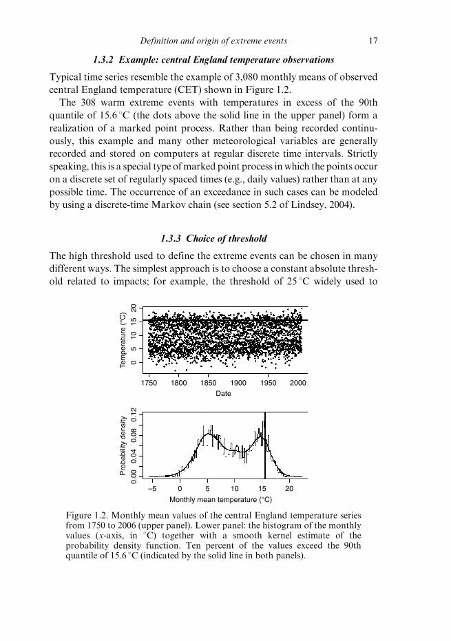
1.3.2 Example: central England temperature observations

Typical time series resemble the example of 3,080 monthly means of observed

central England temperature (CET) shown in Figure 1.2.

The 308 warm extreme events with temperatures in excess of the 90th

quantile of 15.6 8C (the dots above the solid line in the upper panel) form a

realization of a marked point process. Rather than being recorded continu-

ously, this example and many other meteorological variables are generally

recorded and stored on computers at regular discrete time intervals. Strictly

speaking, this is a special type ofmarked point process inwhich the points occur

on a discrete set of regularly spaced times (e.g., daily values) rather than at any

possible time. The occurrence of an exceedance in such cases can be modeled

by using a discrete-time Markov chain (see section 5.2 of Lindsey, 2004).

1.3.3 Choice of threshold

The high threshold used to define the extreme events can be chosen in many

different ways. The simplest approach is to choose a constant absolute thresh-

old related to impacts; for example, the threshold of 25 8C widely used to

2015

105

0

Pro

babi

lity

dens

ity 0.12

0.08

0.04

0.00

Tem

pera

ture

(°C

)

–5 0 5 10 15 20

Monthly mean temperature (°C)

Date

1750 1800 1850 1900 1950 2000

Figure 1.2. Monthly mean values of the central England temperature seriesfrom 1750 to 2006 (upper panel). Lower panel: the histogram of the monthlyvalues (x-axis, in 8C) together with a smooth kernel estimate of theprobability density function. Ten percent of the values exceed the 90thquantile of 15.6 8C (indicated by the solid line in both panels).

Definition and origin of extreme events 17

define extreme heat wave indices (e.g., Alexander et al., 2006; New et al., 2006).

Such extreme events can lead to severe health situations, which are likely

to become more prevalent due to global warming (McGregor et al., 2005).

A more relative approach is to choose a constant threshold based on the

empirical distribution of the variable at each location; for example, the 90th

quantile shown in the central England temperature example. This approach

is useful in that it ensures that a given fraction (e.g., 10%) of events will by

definition be ‘‘extreme.’’ In other words, it defines ‘‘extremeness’’ in terms of

‘‘rarity.’’ In addition to these two approaches, one can also consider time-

varying thresholds. For example, ‘‘record-breaking’’ events can be defined by

choosing the threshold to be the maximum value of all previously observed

values. One can also choose trending thresholds to help take account of non-

stationarities such as the changing baseline caused by global warming. Such

definitions of extreme events can help us avoid the paradoxical situation

whereby ‘‘extreme events will become the norm’’ (as was stated by Deputy

Prime Minister John Prescott after the autumn 2000 UK floods).

1.3.4 Magnitude of the extreme events (distribution of the marks)

The magnitude of the extreme events can most easily be summarized by calcu-

lating summary statistics of the sample of excesses; for example, themean excess

above the threshold (Coles, 2001). However, such an approach does not allow

one to make inferences about as-yet-unobserved extreme values or provide

probability estimates of extreme values that have reliable uncertainty estimates.

It is therefore necessary to fit an appropriate tail probability distribution to

the observed excesses (e.g., the sample of 308 excesses for the CET example).

Under rather general assumptions, a limit theorem shows that for most

continuous random variables, the probability of exceedance above a large

value x > u is given by

PrðX4xjX4uÞ ¼ 1þ � x� u

s

� �h i�1�

for a sufficiently high threshold u. This two-parameter distribution is known as

the generalized Pareto distribution (GPD). The dimensional parameter, s,defines the scale of the excesses, whereas the dimensionless parameter, �,

defines the overall shape of the tail. These two parameters can be easily

estimated by using maximum likelihood estimation.

For the CET example, the excesses above the 90th quantile u ¼ 15:6 8C give

a scale parameter estimate of 1.38 8C (with a standard error of 0.09 8C) and a

shape parameter estimate of � 0.30 (with a standard error of 0.04). The

18 D. Stephenson

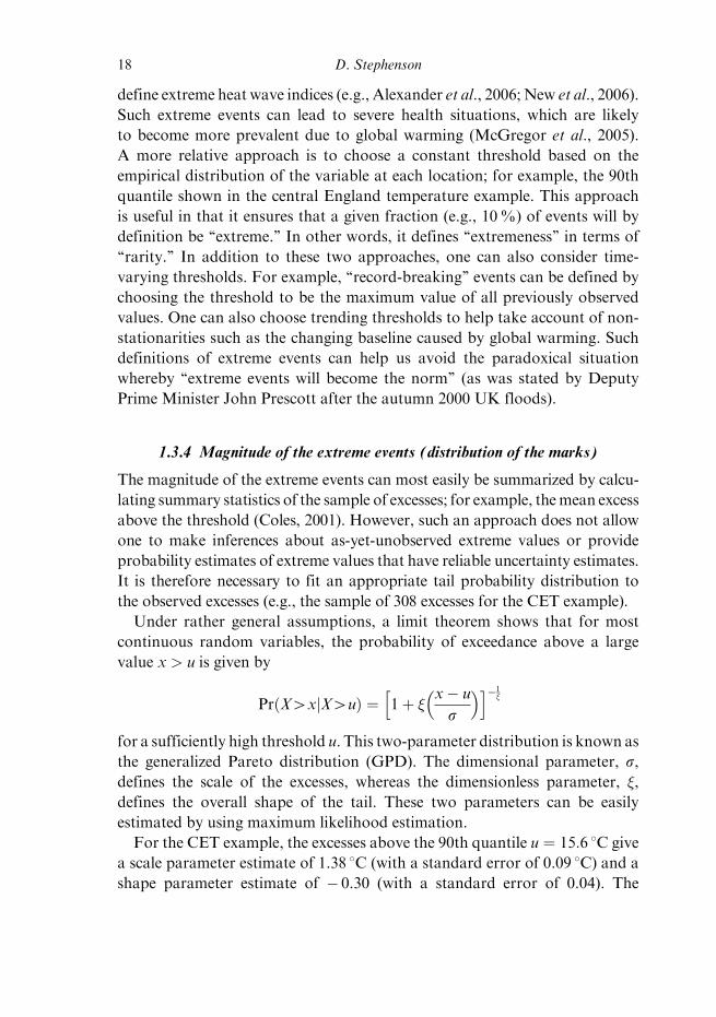
negative shape parameter implies that the tail distribution has an upper limit

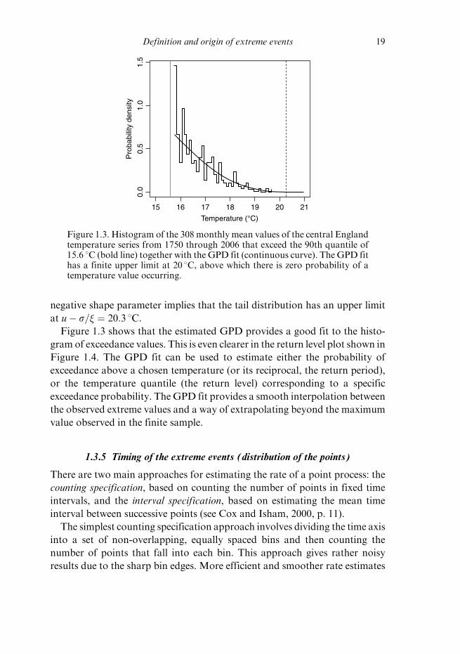
at u� s=� ¼ 20:3 8C.Figure 1.3 shows that the estimated GPD provides a good fit to the histo-

gram of exceedance values. This is even clearer in the return level plot shown in

Figure 1.4. The GPD fit can be used to estimate either the probability of

exceedance above a chosen temperature (or its reciprocal, the return period),

or the temperature quantile (the return level) corresponding to a specific

exceedance probability. The GPD fit provides a smooth interpolation between

the observed extreme values and a way of extrapolating beyond the maximum

value observed in the finite sample.

1.3.5 Timing of the extreme events (distribution of the points)

There are two main approaches for estimating the rate of a point process: the

counting specification, based on counting the number of points in fixed time

intervals, and the interval specification, based on estimating the mean time

interval between successive points (see Cox and Isham, 2000, p. 11).

The simplest counting specification approach involves dividing the time axis

into a set of non-overlapping, equally spaced bins and then counting the

number of points that fall into each bin. This approach gives rather noisy

results due to the sharp bin edges. More efficient and smoother rate estimates

15

1.5

1.0

0.5

0.0

Pro

babi

lity

dens

ity

16 17 18 19 20 21

Temperature (°C)

Figure 1.3. Histogram of the 308 monthly mean values of the central Englandtemperature series from 1750 through 2006 that exceed the 90th quantile of15.6 8C (bold line) together with the GPD fit (continuous curve). The GPD fithas a finite upper limit at 20 8C, above which there is zero probability of atemperature value occurring.

Definition and origin of extreme events 19

can be obtained by using smooth local weighting based on a smooth kernel

function rather than a sharp-edged bin (Diggle, 1985). Such an approach was

recently used to investigate extreme flooding events in eastern Norway as

observed in paleoclimatic lake sediments (Bøe et al., personal communica-

tion). Various tests can be used to test for trends in the rate of a Poisson

process, but these have differing abilities to detect trends (Bain et al., 1985;

Cohen and Sackrowitz, 1993).

In addition to characterizing changes in the rate and magnitude of a point

process, one can also investigate the temporal clustering. For example,Mailier

et al. (2006) used simple point process overdispersion ideas to evaluate the

clustering in transits of extratropical cyclones. They found that there is sig-

nificant clustering of cyclones over Western Europe that can be attributed to

rates varying in time due to the dependence on large-scale flow patterns. In

general, time dependence in rates for an extreme event can lead to clustering.

This is a very interesting area for future research on extreme weather and

climate events.

1.3.6 Some ideas for future work

Statistical analysis of extreme events generally focuses on a given set of

extreme events and tends to neglect how such events came into existence.

20

Ret

urn

leve

l

1918

1716

1 2 5 10 20 50 200 500

Return period

Figure 1.4. Return level plot for the central England temperature series from1750 through 2006. The return period is the reciprocal of the probability of amonthly temperature value exceeding the return level. The crosses denote the308 empirical quantiles and probabilities, and the solid curve is the GPD fit.Note the concavity of the curve, which is characteristic of a tail distributionhaving a negative shape parameter.

20 D. Stephenson

This is a strength in that it makes extreme value techniques more universally

applicable to different areas of science no matter how the extremes formed.

However, this approach also has aweakness in that it ignores information about

the process that led to the extreme events that could help improve inference.

How moderately large events evolve into extreme events can provide clues

into the very nature of the extreme events. The dynamical knowledge about

underlying formation processes should be exploited in the statistical analysis.

1.4 The origin of extreme events

Understanding the processes that lead to the creation of extreme events and

how they might change in the future is a key goal of climate science. To help

tackle the problem of the origin of extremes, I propose two guiding principles.

* The evolutionary principle. Extreme events do not arise spontaneously: instead, they

evolve continuously from less extreme events and they stop evolving to become even

more extreme events.

* The stationary principle. Extremes such as local maxima and minima are quasi-

stationary states in which the rate of change of their amplitude is zero. This

characteristic implies that there is an interesting balance between forcing and

dissipation tendencies for such extreme events.

There are various processes that can give rise to extreme events:

* Rapid growth due to instabilities caused by positive feedbacks; for example, the rapid

growth of storms due to convective and baroclinic instability.

* Displacement of a weather system into a new spatial location (e.g., a hurricane in

Boston) or into a different time period (e.g., a late frost in spring).

* Simultaneous coincidence of several non-extreme conditions (e.g., freak waves

caused by several waves occurring together).

* Localization of activity into intermittent regions (e.g., precipitation in intertropical

convergence zones).

* Persistence or frequent recurrence of weather leading to chronic extremes as caused

by slower variations in the climate system (e.g., surface boundary conditions).

* Natural stochastic/chaotic variation that will lead to more extreme values being

recorded as the time length of the record increases.

Understanding these processes is the key to understanding how extreme

events have behaved in the past and how they might behave in the future.

In addition to being of interest because of their large impacts, extreme events

are worth studying because they can reveal insights into key processes. For

example, investigation of rapidly deepening Atlantic storms (‘‘bombs’’) has

helped improve scientific knowledge of fundamental baroclinic instability

Definition and origin of extreme events 21

mechanisms (explosive cyclogenesis). For numerical weather and climate

models to correctly simulate extreme events, they will need to adequately

represent such processes.

1.5 Conclusion

This chapter has addressed the perplexing issues of how to define and diagnose

extreme events. It has been shown that extreme events are generally complex

entities described by several different attributes: rate of occurrence, magnitude

(intensity), temporal duration and timing, spatial structure, and multivariate

dependencies.

Despite this complexity, extreme weather and climate events are often

described by using only a single variable (e.g., maximum wind speed at land-

fall). Exceedances of such a variable above a high threshold define what is

known as simple extreme events. This simple description of complex events can

be considered to be a realization of a stochastic marked point process. Point

process techniques can be usefully employed to characterize properties of

simple extreme events such as the rate, themagnitude, and temporal clustering.

Despite the societal relevance, estimates and predictions of extreme events

are prone to large sampling uncertainty due to the inherent rarity of such

events. Careful inference is needed to make definitive statements about

extreme events such as the regional changes one is likely to see due to global

warming (e.g., Beniston et al., 2006). Inference can be improved by various

approaches such as extrapolating from less extreme events (e.g., using tail

distributions such as the generalized Pareto distribution), by pooling extreme

events over a spatial region to reduce rarity (e.g., tropical cyclones over all the

tropics), and by relating changes in extremes to changes in mean and variance

(Beniston and Stephenson, 2004; Ferro et al., 2006). Such approaches require

careful statistical modeling that can benefit from insight gained from knowl-

edge of dynamical processes that determine extreme events.

Acknowledgments

I thankRickMurnane andHenryDiaz for invitingme to present these ideas in

the opening seminar at the ‘‘Assessing,Modeling, andMonitoring the Impacts

of Extreme Climate Events’’ workshop in Bermuda, October 13–14, 2005.

Many of the ideas presented here have grown out of exciting discussions that

I have had with colleagues over the past few years; in particular, with Dr Chris

Ferro and Professor Martin Beniston. Finally, but not least, I thank the

reviewers of this chapter for their useful comments.

22 D. Stephenson

References

Alexander, L. V., Zhang, X., Peterson, T. C., et al. (2006). Global observed changes indaily climate extremes of temperature and precipitation. Journal of GeophysicalResearch (Atmospheres), 111, D05109, doi:10.1029/2005JD006290.

Bain, L. J., Engelhardt, M., and Wright, F. T. (1985). Tests for an increasing trend inthe intensity of a Poisson process: a power study. Journal of the AmericanStatistical Association, 80(390), 419–22.

Beniston,M., and Stephenson,D.B. (2004). Extreme climatic events and their evolutionunder changing climatic conditions. Global and Planetary Change, 44, 1–9.

Beniston, M, Stephenson, D. B., Christensen, O. B., et al. (2006). Future extremeevents in European climate: an exploration of regional climate model projections.Climatic Change, PRUDENCE special issue.

Cohen, A., and Sackrowitz, H. B. (1993). Evaluating tests for increasing intensity of aPoisson process. Technometrics, 35(4), 446–8, doi:10.2307/1270277.

Coles, S. (2001). An Introduction to Statistical Modeling of Extreme Values. London:Springer-Verlag.

Cox, D.R., and Isham, V. (2000). Point Processes. New York: Chapman & Hall/CRC.Daley, D. J., and Vere-Jones, D. (2002). An Introduction to the Theory of Point

Processes, 2nd edition. Berlin: Springer-Verlag.Diggle, P. J. (1983). Statistical Analysis of Point Processes. London: Chapman&Hall.Diggle, P. J. (1985). A kernel method for smoothing point process data. Applied

Statistics, 34, 138–7.Ferro, C.A. T., Hannachi, A., and Stephenson, D. B. (2006). Simple non-parametric

techniques for exploring changing probability distributions of weather. Journal ofClimate, 18, 4344–54.

Intergovernmental Panel on Climate Change (IPCC) (2001). Climate Change 2001:Synthesis Report. Cambridge: Cambridge University Press.

Lindsey, J.K. (2004). Statistical Analysis of Stochastic Processes in Time. Cambridge:Cambridge University Press.

Mailier, P. J., Stephenson, D. B., Ferro, C.A. T., and Hodges, K. I. (2006). Serialclustering of extratropical cyclones. Monthly Weather Review, 134(8), 2224–40.

McGregor, G.R., Ferro, C.A. T., and Stephenson, D. B. (2005). Projected changes inextreme weather and climate events in Europe. In Extreme Weather and ClimateEvents and Public Health Responses, ed. W. Kirch, B. Menne, and R. Bertollini.Dresden: Springer, pp. 13–23.

New, M., Hewitson, B., Stephenson, D. B., et al. (2006). Evidence of trends in dailyclimate extremes over southern and west Africa. Journal of Geophysical Research(Atmospheres), 111, D14102, doi:10.1029/2005JD006289.

Definition and origin of extreme events 23