September 2019

DEFINITION MATTERS. METROPOLITAN AREAS AND AGGLOMERATION

ECONOMIES IN A LARGE DEVELOPING COUNTRY

Maarten Bosker, Jane Park, and Mark Roberts

BACKGROUND PAPER

Urbanization Flagship Report

Time to ACT: Realizing Indonesia’s Urban Potential

Pub

lic D

iscl

osur

e A

utho

rized

Pub

lic D

iscl

osur

e A

utho

rized

Pub

lic D

iscl

osur

e A

utho

rized

Pub

lic D

iscl

osur

e A

utho

rized

1

Definition Matters. Metropolitan Areas and Agglomeration Economies in a Large Developing Country1

Maarten Bosker2, Jane Park3, and Mark Roberts4

September 2018

Abstract

A variety of approaches to delineate metropolitan areas have been developed. Systematic comparisons

of these approaches in terms of the urban landscape that they generate are however few. Our paper

aims to fill this gap. We focus on Indonesia and make use of the availability of data on commuting

flows, remotely-sensed nighttime lights, and spatially fine-grained population, to construct metropolitan

areas using the different approaches that have been developed in the literature. We find that the maps

and characteristics of Indonesia’s urban landscape vary substantially depending on the approach used.

Moreover, combining information on the metro areas generated by the different approaches with

detailed micro-data from Indonesia’s national labor force survey, we show that the estimated size of

the agglomeration wage premium depends nontrivially on the approach used to define metropolitan

areas.

Key words: metro areas, urban definitions, agglomeration economies, Indonesia

JEL Codes: O18, O47, C21

1 This paper has been prepared as a background paper to the World Bank’s Indonesia Urbanization Flagship report, Time to

ACT: Realizing Indonesia’s Urban Potential. The authors thank Katie McWilliams, Benjamin Stewart and Andrii Berdnyk for

their outstanding GIS support, as well as Brian Blankespoor and Shaun Zhang for supplemental GIS support. The findings,

interpretations, and conclusions expressed in this paper are entirely those of the authors. They do not necessarily represent

the views of the International Bank for Reconstruction and Development/World Bank and its affiliated organizations, or

those of the Executive Directors of the World Bank or the governments they represent. The work received financial support

from the Swiss State Secretariat for Economic Affairs (SECO) through the Indonesia Sustainable Urbanization Multi-Donor

Trust Fund (IDSUN MDTF). Financial support from DFID is also gratefully acknowledged. 2 Department of Economics, Erasmus University Rotterdam, The Netherlands and CEPR <bosker@ese.eur.nl> 3 Urban, Resilience and Land Global Practice, The World Bank, Washington, DC, USA <jpark16@worldbank.org> 4 Urban, Resilience and Land Global Practice, The World Bank, Singapore office <mroberts1@worldbank.org>

(corresponding author).

2

1. Introduction

Traditionally, urban economists have, except for the US for which data on metropolitan statistical

areas (MSAs) is readily available, relied on data for cities as defined by their administrative boundaries.

However, administrative boundaries often fail to adequately delineate the “true” boundaries of a city,

leading to cities being, sometimes substantially, “under-” or “over-bounded” (administrative

boundaries under- or, respectively, overstating the true city area). This issue has been highlighted for

developing and developed countries alike, especially in situations where urbanization has been rapid

and cities have been growing quickly in terms of not only population, but also in the land area which

they cover (see, for example, Ellis and Roberts, 2016).

In reaction to this, there have been a growing number of attempts in recent years to develop and

apply algorithms that enable the better delineation of cities and metropolitan areas. These attempts

have been led not just by economists, but also by both geographers and the remote sensing

community, in which there is a very long tradition of using satellite imagery to help define a city’s

“true” extent (see, for example, Danko, 1992; Elvidge et al., 1996). Moreover, many of them have been

driven by international organizations such as the Development Bank of Latin America (CAF), The

European Commission (EC), the Organization for Economic Co-operation and Development (OECD),

and The World Bank. The ambition of these organizations has been to construct consistently defined

global data sets of cities to facilitate the uniform measurement of urbanization.5

While the preferred approach of economists to defining cities and metropolitan areas tends to be

rooted in a labor market perspective based on the use of commuting flow data, as with the definition

of MSAs in the US, such data is hard to come by for many countries in the world, especially for many

developing countries. As such, attempts to define globally consistent data sets of cities based on the

“true” extents of these cities have instead relied on either the use of estimated travel times to

5 The development of global data sets of cities based on their “true” extents has been greatly facilitated by the increased

availability of global satellite imagery, both optical and nighttime, and the derivation from this imagery of global data sets

of built-up area, including the Global Human Settlement Layer (https://ghsl.jrc.ec.europa.eu/about.php) and the Global

Urban Footprint (https://www.dlr.de/eoc/en/desktopdefault.aspx/tabid-9628/16557_read-40454/) built-up area data sets. It

has also been facilitated by the development of increasingly accurate globally gridded population data.

3

approximate commuting sheds (World Bank, 2008; Uchida and Nelson, 2009; Ellis and Roberts, 2016);

approaches that associate cities with dense clusters of population (Dijkstra and Poelman, 2014;

Roberts, 2018b); or approaches that rely on global satellite imagery and which identify cities based on

their built-up area or the amount of light they emit at night (Ellis and Roberts, 2016; CAF, 2017).

While, however, much effort has been expended in developing and applying algorithms and

approaches for the better delineation of cities and metro areas, little effort has been made to

systematically compare these approaches in terms of the results that they yield (e.g., in the number of

metro areas identified, or in the populations and areas of those metros).6 There has likewise been little

effort to compare the results of “second best” approaches to defining metro areas – i.e. approaches

which rely on global data sets and which proxy or otherwise forego the use of commuting flow data –

with the economist’s “first best” approach based on the identification of a city’s functional area using

data on origin – destination (O-D) commuting flows. At the same time, while international

organizations have developed global maps of consistently defined cities, there has been no effort to

explore how the use of these maps to define cities affects key empirical results that are crucial to a

proper understanding of the working of urban economies, such as, for example, the estimated

strength of agglomeration economies.

Given the above, the aims of this paper are two-fold. First, we compare the results of different

algorithms and approaches for delineating metropolitan areas in terms of the basic descriptions they

provide of the urban landscape (notably, the number of metro areas, the sub-national administrative

units that these areas cover, and their population sizes). And, second, we assess whether the choice of

approach to defining metro areas matters when it comes to estimating the strength of agglomeration

economies.

More specifically, we compare four different approaches. The first of these requires O-D commuting

flow data and adheres to the economist’s preferred approach of defining metro areas as functional local

labor markets. Specifically, for this first approach, we make use of an algorithm recently developed by

6 Exceptions are Rozenfield et al. (2011) who, for the United States, compare results derived from a population clustering

algorithm for identifying cities with cities as defined by their MSAs, and Roberts et al. (2017), who compare the maps

associated with three different global approaches to delineating urban areas.

4

Duranton (2015b). The other three approaches are “second best” approaches which instead rely on

global data sets derived, wholly or in part, from satellite imagery. These three approaches are the

Agglomeration Index (AI), which was originally developed by Uchida and Nelson (2009) for the World

Bank’s 2009 World Development Report on “Reshaping Economic Geography” (World Bank, 2008); a

“Cluster Algorithm” developed by Dijkstra and Poelman (2014) which associates cities with dense

clusters of population; and, finally, the identification and delineation of metro areas based on the

“thresholding of Night-Time Lights data” (NTL), similar to, for example, Ellis and Roberts (2016) and

CAF (2017). These latter three approaches all have the obvious advantage that they can be applied to

any country in the world using readily available data sets, including those countries for which O-D

commuting flow data is not available.

In all our empirics, we focus on the case of a single large developing country – Indonesia. Unlike

many developing countries, Indonesia has the advantage that its national labor force survey (Survei

Tenaga Kerja Nasional, SAKERNAS) allows for the derivation of an O-D matrix of commuting flows

between sub-national areas (districts), which is the crucial input for the application of the Duranton

(2015b) algorithm in defining metro areas. Beyond the main focus of this paper, however, Indonesia’s

urban landscape is interesting to study in and of itself. Indonesia has, in recent decades, been one of

the world’s most rapidly urbanizing countries and, within the country, there is intense policy interest in

the issue of how to delineate metropolitan areas (see, World Bank, forthcoming). By focusing on

Indonesia, our paper also contributes to the, to date, limited credible empirical evidence on the

strength of agglomeration economies in developing countries. This is a knowledge gap that

economists such as Overman and Venables (2005), Duranton (2015a), and Glaeser and Henderson

(2017) have made recent calls for the profession to fill.

The remainder of our paper is structured as follows. Section 2 describes the four approaches for

delineating metropolitan areas that we compare in this paper. Section 3 presents our application of

these approaches to Indonesia. We document the data that we use to implement these approaches,

and present a basic descriptive comparison of Indonesia’s urban landscape generated by the different

approaches. Section 4 then takes the definitions of metro areas from Section 3 to see whether the

5

choice of definition makes a difference for the estimated strength of agglomeration economies.

Section 5 concludes.

2. Approaches to Defining Metro Areas

The four approaches to defining metro areas that we compare in this paper are:

Approach #1: Local labor market approach – Duranton (2015b) algorithm

This approach identifies a metropolitan area as an integrated local labor market. All else equal in

terms of data availability, such a functional approach to defining a city, is typically preferred by

economists. Duranton (2015b)’s algorithm holds the advantage over other algorithms that similarly

seek to delineate metro areas based on their functional areas in that it does not require the pre-

definition of metro cores nor the use of additional criteria beyond the specification of a simple

commuting flow threshold (Duranton, 2015b). The algorithm is a simple iterative algorithm which uses

sub-national administrative units (in our case, Indonesian districts) to “grow” metro areas through

successive aggregation.

In the first round of running the algorithm, a district A will be aggregated to a second district, B, if the

share of workers that live in A and commute daily for work to B is above a given threshold, �̅�. In the

second round, the algorithm will then aggregate a third district, C, to the union of A and B, if the

share of workers that live in C and commute daily to the spatial unit A + B exceeds �̅�, even though it

may not have been possible to aggregate C to either A or B directly in round one. The algorithm then

continues to run until no districts remain to be aggregated given the commuting flow threshold.7

Based on his own application of the algorithm to Colombian municipalities, Duranton (2015b) notes

that, given the gravitational nature of commuting, the algorithm’s preferred threshold for any

application is likely to be decreasing in the sizes of the underlying sub-national units being

aggregated into metropolitan areas.

7 Prior to aggregating a given origin district to a given destination district, the algorithm checks that in cases where a district

could be aggregated to several destinations, it is, in fact, uniquely added to the one to which it sends the greatest number

of workers. When commuting flows between two districts are above the threshold in both directions, the algorithm also

ensures that the smaller district is aggregated to the larger. (see, Duranton, 2015b, p 184).

6

Approach #2: The Agglomeration Index (AI)

The Agglomeration Index (AI) was originally developed by Uchida and Nelson (2009) for the World

Bank’s 2009 World Development Report (WDR) on “Reshaping Economic Geography” and, since then,

has been further applied in other World Bank reports, including in World Bank – IMF (2013) and Ellis

and Roberts (2016). The AI was designed by Uchida and Nelson for global application. Given the

absence of O-D commuting flow data for many countries – especially developing countries – it

instead relies on estimated travel times to a set of pre-defined cores to delineate the extents of metro

areas. Cores are pre-defined from a global settlement point layer8 based on a population threshold.

Rather than rely on sub-national administrative units, the AI instead relies on a globally gridded

population data set. In such a data set, the underlying units that undergo aggregation are grid cells

that are of a uniform geographic size – in practice, 30-arc seconds, which is approximately 1 km2 at

the equator.

Constructing the AI first requires the specification of three thresholds – a minimum population

threshold to identify settlement points that qualify as metro cores, a travel time threshold, and a

population density threshold. While Uchida and Nelson (2009) experimented with a range of

thresholds, the AI has become synonymous with thresholds of 50,000 for the population of the core,

60 minutes for travel time, and 150 people per km2 for population density. Hence, the AI defines a

group of population grid cells as constituting a metro area if each of those grid cells have a

population density of at least 150 people per km2 and fall within a 60-minute travel time radius of a

settlement point that has an associated population of at least 50,000. An important feature of the AI is

that it, in contrast to the other two “satellite data based” approaches, does not include a contiguity

requirement. This means that, in principle, a metro area may not consist of a single contiguous block

of grid cells. Another important feature of the AI is that if there are two or more cores that fall within

60 minutes travel time of each other then they, effectively, merge into a single extended metro area.

8 Namely, CIESIN’s Global Rural – Urban Mapping Project (GRUMP) Settlement Point layer

(http://sedac.ciesin.columbia.edu/data/set/grump-v1-settlement-points-rev01).

7

Approach #3: The cluster algorithm

Rather than attempting to delineate a metro area based on its functional area, using either

commuting flow data or estimated travel times, Dijkstra and Poelman’s (2014) cluster algorithm simply

identifies a metro area as a dense population cluster. The algorithm was originally developed with the

European Union in mind, but has since been applied globally and, given the simplicity of its data

requirements, is emerging as the preferred algorithm of not only the European Commission, but also

of a coalition of international agencies that further includes the Organization for Economic

Cooperation and Development (OECD) and the World Bank. As with the AI, the cluster algorithm

relies on a gridded population data set of resolution 30 arc-seconds – i.e. approximately 1 km2 at the

equator – as input. Given this data, it identifies a spatially contiguous set of population grid cells as a

metro if each of those grid cells satisfies a population density threshold, �̅�𝐷, and, collectively, the

population of the grid cells exceeds a population threshold, �̅�𝑃.

In practice, the cluster algorithm has become associated with two different sets of thresholds. The first

set of thresholds is �̅�𝐷 = 300 people per km2 and �̅�𝑃 = 5,000 with the resultant areas that are

delineated being referred to as “Urban Clusters” (UC). Meanwhile, the second set of thresholds is �̅�𝐷 =

1,500 people per km2 and �̅�𝑃 = 50,000 with the areas that result being labelled “High Density

Clusters” (HDC) (Dijkstra and Poelman, 2014).

Approach #4: Thresholding of night-time lights (NTL) data

The use of night-time lights (NTL) data to identify metro areas, and, more generally, urban

settlements, originated in the remote sensing literature with early applications including Imhoff et al.

(1997), Sutton (2003), and Small et al. (2005). More recent applications at either a regional or a global

scale include Zhang and Seto (2011), Zhou et al. (2015), Ellis and Roberts (2016), and CAF (2017).

Applications of NTL data to delineate metro areas have invariably relied on data products that have

been derived by the National Oceanic and Atmospheric Association (NOAA) from sensors (Optical

Line Scanner, or OLS, sensors) on-board the Defense Meteorological Satellite Program (DMSP)

constellation of satellites. The derived DMSP-OLS data products cover the entire globe and are

available at a resolution of 30 arc-seconds, which is, again, equivalent to approximately 1 km2 at the

equator. One deficiency of DMSP-OLS NTL data, however, is that it suffers from a well-documented

8

“overglow” or “blooming” problem, whereby the light emitted from a given point on the earth is

recorded as covering an area that extends beyond that point.9 This creates a tendency for the lit area

of a metro to overstate its “true” extent – for example, the Pacific Ocean can be lit up as far as 50 km

from the coastline near Los Angeles (Pinkovskiy, 2013). The most common approach to dealing with

this overglow problem has been to threshold the NTL data, considering only pixels in the data that

exceed a certain luminosity, or digital number (DN), value as part of the area of a city or metro (see,

for example, Imhoff et al., 1997; Small et al., 2005; Zhou et al., 2015; Ellis and Roberts, 2016). A

contiguous cluster of grid cells that falls above the applied threshold is then classified as constituting a

“metro” area.

More recently, however, DMSP-OLS NTL data has been superseded by NTL data collected from a

new satellite sensor, the Visible Infrared Imaging Radiometer Suite (VIIRS) sensor, launched in 2011.

This sensor collects NTL data at a far higher resolution than the old DMSP-OLS sensors and the

derived data products are also not subject to the overglow problem. We use the new VIIRS satellite

data to delineate metro areas. Specifically, we use the 2015 annual composite product which has

recently been released by NOAA.10 This product reports luminosity values, calculated as an annual

average over all cloud-free nights in 2015, at a resolution of 15 arc seconds, which is equal to 460 m2

at the equator. Prior to averaging, NOAA applies filtering techniques to remove data that is affected

by stray light, lightning, and lunar illumination. NOAA likewise filters out lights from aurora, fires, boats

and other temporary lights. Although the VIIRS NTL data does not suffer from the same overglow

problem as the DMSP-OLS NTL data, it, nevertheless, records light emitted to the nighttime sky by all

human activities, including light at very low levels outside of what may be considered metro or even

urban areas. For this reason, the use of a threshold may still be required to properly delineate metro

from non-metro areas. As with papers that have used the DMSP-OLS data for the same purpose, we

consider a contiguous cluster of grid cells that falls above any imposed threshold as representing a

“metro” area.

9 See Doll (2008) for a description of the underlying causes of the overglow problem with DMSP-OLS NTL data. 10 This product is available for download from: https://ngdc.noaa.gov/eog/viirs/download_dnb_composites.html.

9

3. Application to Indonesia

3.1. Data sources

The data that we use to apply the four approaches to delineating metro areas to Indonesia come

from a variety of sources. For Duranton’s algorithm, we use data on O-D commuting flows between

Indonesian districts that we derive from the August rounds of Indonesia’s national labor force survey

(Survei Tenaga Kerja Nasional, SAKERNAS) for the years 2013 – 2015.11 In doing so, we measure the

commuting flow from a given origin district i to a destination district j as the share of workers who live

in i but commute daily to work in j, where – following SAKERNAS – workers are defined to include all

employed wage workers including casual workers, self-employed workers, and unpaid family workers,

where anyone who worked for at least one hour consecutively in the previous week, including

temporary non-workers who normally meet the condition, is considered employed.

Both the AI and the two cluster algorithms require a gridded population data set. We use the

Landscan-2012 gridded population data set produced by Oak Ridge National Laboratory. This

population grid has a resolution of 30 arc-seconds. An earlier version of the same population grid

was used by Uchida and Nelson (2009) in their original application of the AI. More generally, the

Landscan population grid is the most established global gridded population data set and has been

widely used in social scientific research.12 This includes the paper by Henderson et al. (2018), who use

the same Landscan-2012 data in identifying urban areas and for constructing measures of population,

and economic, density for six African countries. Importantly, Henderson et al. (2018) “ground-truth”

the Landscan data, reaching the conclusion that it does good job in estimating population at a fine

spatial scale. The population grid is derived through distributing population data for sub-national

11 Importantly, the sampling strategy of the SAKERNAS August rounds is stratified at the district level for these years. We

average the commuting flows over three years, rather than using a single year, to smooth-out any temporary measurement

error in the survey data. 12 Alternative population grids that we could have used are WorldPop (http://www.worldpop.org.uk/) and GHS-Pop

(http://ghsl.jrc.ec.europa.eu/ghs_pop.php). Roberts et al. (2017) compare the level of agreement between maps of urban

areas generated using the AI and cluster algorithms with different gridded population products. In general, the level of

agreement is fairly high.

10

administrative units across grid cells using a modelling process that relies on other geo-spatial data

sources and high-resolution satellite imagery analysis.13

In addition to gridded population data, the AI also requires data on estimated travel times. The travel

time data originally used by Uchida and Nelson (2009) for the AI was based on “… estimates of the

time required to travel 1 km over different road and off-road surfaces…” and was derived from a cost

surface that was constructed from a variety of Geographic Information System (GIS) data layers.

These layers included data on road and rail networks, navigable rivers and water bodies, travel delays

for crossing international borders, roughness of terrain and foot based travel for off-road and paths.14

The AI estimates used in this paper are taken from Roberts et al. (2017) and based on an updated

version of this same cost surface layer from Berg et al. (2017). This updated layer is derived from

more recent (i.e. circa 2010 versus circa 2000) data on roads, railroads, and land cover.15

Finally, as already described in Section 2, the NTL data that we use in this paper is VIIRS NTL data

taken from NOAA’s 2015 annual composite product.

3.2. Mapping to Districts

One issue that we face in generating results that can be compared across the different approaches

for delineating metro areas is that while Duranton’s algorithm uses sub-national administrative units –

in our case, Indonesian districts – as the “building blocks” for metro areas, the remaining approaches

rely on much higher resolution gridded data sets. This means that while the outer perimeters of the

metro areas defined by Duranton’s algorithm are constrained to follow district boundaries, this is not

the case for the metro areas generated by the other approaches. The latter is, in principle, a highly

attractive feature of using the AI, cluster algorithm or NTL data to define metro areas. But,

importantly, it poses difficulties for any empirical analysis that wishes to use the metro areas based on

13 See http://web.ornl.gov/sci/landscan/landscan_documentation.shtml for more information. 14 See Appendix Table A.1 in Uchida and Nelson (2009) for more details. 15 One important limitation of the resultant travel time estimates is that they do not take account of travel time delays owing

to traffic congestion.

11

these approaches as the unit of observation. This is because other data that the researcher might wish

to match to these metro areas with will often only be available for sub-national administrative areas

or, in the case of household and firm survey micro-data, include location identifiers for such areas

only, or has been obtained using a random sampling strategy stratified at the level of sub-national

administrative areas. This is also the case for Indonesia.

Given the above, we need to map the urban extents generated by the AI, cluster algorithm and NTL

approach to (aggregations of) Indonesian districts. We do this by always applying the same basic rule:

we associate two or more districts with a single urban extent if at least 50 percent of the district’s

population belongs to that urban extent. In this way, we construct approximations of the “true” urban

extents implied by a given approach through the aggregation of districts.16 Analogous to Duranton’s

algorithm, we only consider a given urban extent generated by each of the AI, cluster algorithm and

NTL approach to represent a metro area if that extent maps to two or more districts. This implies, for

example, that where an urban extent is smaller in area than a district, we do not consider this to be a

metropolitan area.17

The Indonesian districts in our analysis are defined by their official 2013 boundaries. On average, such

districts are large. The median area of an Indonesian district in our data is 1,943 km2 with a range that

goes from a minimum of 9.6 km2 to a maximum of 44,177 km2. However, 76.4 percent of Indonesia’s

urban population in 2014 lived in districts of below median area, while 53 percent lived in districts of

area less than 1,000 km2. As shown in Figure 1 in Section 3.3 below, despite the large average size of

16 We have experimented with the sensitivity of our results to the 50 percent threshold by increasing it, in steps of 5

percentage points, up to 80 percent. As one might expect, increasing the threshold tends to primarily lead to excluding an

increasing number of districts on the peripheries of the identified metro areas such that they become composed of fewer

districts. This is particularly the case for the AI, the cluster algorithm with the urban cluster set of thresholds, and the NTL

approach with a low luminosity threshold for identifying metro areas. The number of identified multi-district metro areas

itself also falls when increasing the threshold but to a lesser extent (and may even go up when using a higher threshold

“breaks” a metro area identified using a lower threshold in two. Figure A1 in the Appendix illustrates this for the AI, HDC, UC

and two NTL based approaches to define metro areas. Importantly, using a higher threshold does not, qualitatively, affect

any of our main findings in the next Sections. See e.g. Table A10 in the Appendix. 17 This does not mean that we completely discard all districts that are home to urban extents that are wholly contained within

their boundaries. We do include such “single-district urban areas” in our regressions that estimate the agglomeration wage

premium (see Section 4 for more detail).

12

Indonesian districts, the maps of metro areas generated using the different approaches appear to

map very well to districts.

3.3. Key Descriptive Statistics of the Identified Metro Areas

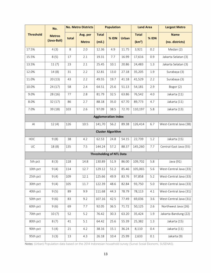
Table 1 summarizes key statistics for metro areas delineated by each of the four approaches. For

Duranton’s algorithm, we present statistics for commuting flow thresholds between 27 percent –

which is when the first metro area appears using this algorithm – and 7 percent. Although we

generated results for all commuting flow thresholds between these two values at 0.5 percent intervals,

we only show results for selected thresholds. Meanwhile, for the cluster algorithm, we show results

based on both the “Urban Cluster” (UC) set of thresholds (i.e. �̅�𝐷 = 300 people per km2, �̅�𝑃 = 5,000)

and the “High Density Cluster” (HDC) set of thresholds (�̅�𝐷 =1,500 people per km2 and �̅�𝑃 = 50,000).

Finally, for the NTL approach, we present selected results based on the thresholding of the lights data

at different points in the distribution of luminosity values.18 In presenting results, we include

information not only on the total number of metro areas, but also on the number of metro areas that

belong to the official island-region of Java-Bali, which is where the majority of Indonesia’s urban

population – approximately 70 percent in 2016 – resides and which, overall, is significantly more

urbanized and densely populated than Indonesia’s other island-regions.19

Table 1. Comparison of key statistics

Threshold

No.

Metros

(Java-Bali)

No. Metro Districts Population Land Area Largest Metro

total Avg. per

Metro

Total

(mil.) % IDN Urban

Total

(km2) % IDN

Name

(no. districts)

Duranton Algorithm

27.0% 1 (1) 2 2.0 3.05 1.2 3.05 191 0.0 Bandung (2)

23.0% 2 (2) 4 2.0 6.71 2.7 6.71 513 0.0 Jakarta Selatan (2)

21.0% 3 (2) 6 2.0 10.88 4.3 10.40 3,405 0.2 Medan (2)

18 For the NTL approach, we experimented with a total of 19 thresholds by breaking the national range of NTL intensity

values (from 0 to 1,340.44) at every 5th percentile. Despite the wide range, low values are prevalent in Indonesia and 95

percent of the values fall below 9.11. 19 In 2016, 60.8 percent of Indonesia’s population was classified as urban. For Indonesia’s other main island-regions, the

shares of the population classified as urban were as follows: Kalimantan (43.5 percent), Sumatra (40.2 percent), Sulawesi

(35.0 percent), Nusa Tenggara (31.6 percent), and Maluku-Papua (31.3 percent).

13

Threshold

No.

Metros

(Java-Bali)

No. Metro Districts Population Land Area Largest Metro

total Avg. per

Metro

Total

(mil.) % IDN Urban

Total

(km2) % IDN

Name

(no. districts)

17.5% 4 (3) 8 2.0 12.36 4.9 11.75 3,921 0.2 Medan (2)

15.5% 8 (5) 17 2.1 19.31 7.7 16.99 17,616 0.9 Jakarta Selatan (3)

13.5% 11 (7) 23 2.1 25.45 10.1 20.86 24,483 1.3 Jakarta Selatan (3)

12.0% 14 (8) 31 2.2 32.81 13.0 27.18 35,205 1.9 Surabaya (3)

11.0% 20 (13) 43 2.2 49.55 19.7 41.18 41,529 2.2 Surabaya (3)

10.0% 24 (17) 58 2.4 64.51 25.6 51.13 54,181 2.9 Bogor (2)

9.0% 28 (16) 77 2.8 81.79 32.5 63.86 76,542 4.0 Jakarta (11)

8.0% 32 (17) 86 2.7 88.18 35.0 67.70 89,773 4.7 Jakarta (11)

7.0% 39 (18) 103 2.6 97.09 38.5 72.70 110,197 5.8 Jakarta (13)

Agglomeration Index

AI 12 (4) 126 10.5 141,70 56.2 89.38 126,414 6.7 West-Central Java (38)

Cluster Algorithm

HDC 9 (8) 38 4.2 62.53 24.8 54.15 22,739 1.2 Jakarta (15)

UC 18 (8) 135 7.5 144.24 57.2 88.37 145,260 7.7 Central-East Java (55)

Thresholding of NTL Data

5th pct 8 (3) 118 14.8 130.89 51.9 86.00 109,702 5.8 Java (91)

10th pct 9 (4) 114 12.7 129.12 51.2 85.46 105,065 5.6 West-Central Java (33)

25th pct 9 (4) 109 12.1 125.66 49.9 83.76 97,858 5.2 West-Central Java (33)

30th pct 9 (4) 105 11.7 122.39 48.6 82.84 93,750 5.0 West-Central Java (33)

40th pct 9 (5) 89 9.9 111.68 44.3 78.79 78,113 4.1 West-Central Java (31)

50th pct 9 (6) 83 9.2 107.16 42.5 77.49 69,036 3.6 West-Central Java (31)

60th pct 9 (6) 69 7.7 92.05 36.5 71.72 50,125 2.6 Northwest Java (26)

70th pct 10 (7) 52 5.2 76.42 30.3 63.20 35,424 1.9 Jakarta-Bandung (22)

80th pct 8 (7) 41 5.1 64.42 25.6 55.39 25,382 1.3 Jakarta (15)

90th pct 5 (4) 21 4.2 38.16 15.1 36.24 8,110 0.4 Jakarta (11)

95th pct 3 (3) 13 4.3 26.18 10.4 25.99 2,633 0.1 Jakarta (9)

Notes: (Urban) Population data based on the 2014 Indonesian household survey (Survei Sosial Ekonomi, SUSENAS).

14

3.3.1 Duranton Algorithm

As expected, the number of metro areas, the total number of districts that compose those metro

areas, the total (urban) population living in metros, as well as the total land area covered by them, all

steadily increase as the commuting flow threshold is lowered from 27 percent to 7 percent. At a

threshold of 27 percent, we find a single metro area (Bandung) comprised of two districts that has an

entirely urban population of just over 3 million and an area of 191 km2. A second metro area (Jakarta

Selatan), also comprising two districts, then appears at a threshold of 23 percent, more than doubling

the overall urban population that lives in metro areas to 6.7 million and the total land area covered by

metro areas to 513 km2. By the time the threshold reaches 10 percent, which is Duranton’s preferred

threshold in his application to Colombia, the number of metro areas has increased to 24, 17 of which

are located on Java – Bali. The aggregate population of these metro areas is 64.5 million (25.6

percent of Indonesia’s population) with an urban population of 51.1 million. Together, the metro areas

cover just over 54,000 km2 or 2.2 percent of Indonesia’s total land area. At the lowest threshold of 7

percent, the number of metro areas has reached 39, 18 of which are on Java – Bali, with an aggregate

population of 97 million and an overall urban population of 72.7 million. These metro areas

collectively cover 110,197 km2.

Interestingly, regardless of the threshold used, the average number of districts per metro area

remains small, increasing steadily from two at a threshold of 27 percent to 2.8 at a threshold of 9

percent before subsequently declining to 2.6 at a threshold of 7 percent. This turns out to be a

defining feature of this approach: reducing the commuting threshold mainly has the effect of

increasing the number of metro areas rather than the spatial extent of those metro areas. Finally, it is

also notable that only as the threshold is lowered below 10 percent, more and more metros start

appearing outside of Java – Bali. Using the 10% threshold identifies 24 metro areas of which 17 are on

Java-Bali. Reducing the threshold further from 10 to 7 percent adds fifteen additional metro areas, of

which only 1 is on Java – Bali (see also Figure A2 in Appendix A). Also, it is not until a threshold of 9

percent that the five constituent districts of DKI Jakarta – which is the recognized core of Indonesia’s

capital city – aggregate into a single metro area. And, only at the lowest threshold of 7 percent does

15

Duranton’s algorithm aggregate the districts that belong to Jabodetabek, the official Jakarta

metropolitan area (see also Figure 1b).

3.3.2 The Agglomeration Index (AI)

The AI approach generates highly implausible results at the standard thresholds with which it has

become synonymous (i.e. a core population of 50,000, a travel time radius of 60 minutes, and a

population density threshold of 150 people per km2).20 It yields 12 metro areas with an aggregate

population of 141.6 million (equivalent to 56.2 percent of the Indonesian population), of which 89.4

million is urban. Out of these 12 metro areas, however, only four are located on Java – Bali. The small

number of metros on Java – Bali is a consequence of the low population and population density

thresholds associated with the AI, as well as the fact that cores that are within 60 minutes travel time

of each other merge together in extended metro areas. Given that Java – Bali, overall, is very densely

populated, this results in a small number of exceptionally large metro areas. The low population

density threshold results in the algorithm picking-up development along Indonesia’s major roads that

connect cities, contributing to the grouping together of large numbers of districts. As Figure 1c shows,

the largest metro generated by the AI covers much of West and Central Java and consists of 38

districts with a total aggregate population of 63 million, which is more than double the population of

the largest metro generated by Duranton’s algorithm at the 7 percent threshold, which corresponds

to the official Jabodetabek area and consists of only 13 districts.

3.3.3 The Cluster Algorithms

A similar story to that for the AI holds for the cluster algorithm under the Urban Cluster set of

thresholds (i.e. �̅�𝐷 = 300 people per km2, �̅�𝑃 = 5,000). With these thresholds we obtain an aggregate

metro population – 144.2 million (equivalent to 57.2 percent of Indonesia’s overall population) – that

is remarkably close to that generated by the AI. This population is spread over 135 districts which form

18 separate metro areas, eight of which are located on Java – Bali (Table 1). Again, the largest metro,

20 Of course, the approach may potentially yield more plausible results if different thresholds are applied or if delays due to

traffic congestion are incorporated into the travel time estimates.

16

which, in this case, covers much of East and Central Java, is implausibly large. Thus, it covers 38

districts with a total population of 53.7 million (Figure 1d).

When we turn, however, to the cluster algorithm with the High-Density Cluster set of thresholds (i.e.

�̅�𝐷 =1,500 people per km2 and �̅�𝑃 = 50,000), the results look more reasonable (Figure 1(e)). The most

populous metro area in this case corresponds, in a recognizable manner, to Jakarta; although, with 33

million people, it has a slightly larger population that the official Jabodetabek area that Duranton’s

algorithm successfully replicates when using a commuting threshold of 7 percent. Meanwhile, the

overall population that lives in metro areas is 62.5 million, which is close to Duranton’s algorithm at a

threshold of 10 percent (Table 1). Compared to Duranton’s algorithm at this threshold, however, the

total number of metro areas is far fewer (9 versus 24) and the average number of districts per metro

area correspondingly larger (4.2 versus 2.4).

Figure 1. Selected maps for metro areas defined by different approaches (Java – Bali only)

(a) Duranton’s algorithm – 10%

(b) Duranton’s algorithm – 7%

(c) Agglomeration Index (d) Cluster Algorithm – Urban Cluster

17

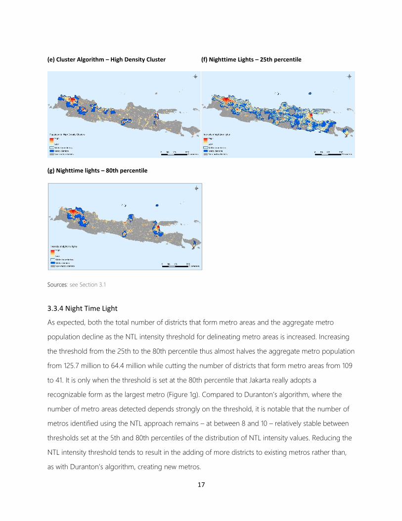
(e) Cluster Algorithm – High Density Cluster

(f) Nighttime Lights – 25th percentile

(g) Nighttime lights – 80th percentile

Sources: see Section 3.1

3.3.4 Night Time Light

As expected, both the total number of districts that form metro areas and the aggregate metro

population decline as the NTL intensity threshold for delineating metro areas is increased. Increasing

the threshold from the 25th to the 80th percentile thus almost halves the aggregate metro population

from 125.7 million to 64.4 million while cutting the number of districts that form metro areas from 109

to 41. It is only when the threshold is set at the 80th percentile that Jakarta really adopts a

recognizable form as the largest metro (Figure 1g). Compared to Duranton’s algorithm, where the

number of metro areas detected depends strongly on the threshold, it is notable that the number of

metros identified using the NTL approach remains – at between 8 and 10 – relatively stable between

thresholds set at the 5th and 80th percentiles of the distribution of NTL intensity values. Reducing the

NTL intensity threshold tends to result in the adding of more districts to existing metros rather than,

as with Duranton’s algorithm, creating new metros.

18

Summarizing, the different approaches to delineating metro areas generate often very different

results in terms of, inter alia, the number of metro areas, the aggregate population of those metro

areas, and the characteristics of the largest identified metro area. Both the AI and the cluster

algorithm under the urban cluster set of thresholds generate results that appear implausible. This is

because their low population density thresholds contribute to generating implausibly large metro

areas – in both cases, almost the entirety of Java – Bali is split into a small number of metros, as is

most evident from Figures 1c and 1d. Results look more reasonable under the other approaches. Most

notably, at a commuting flow threshold of 7 percent, Duranton’s algorithm – which represents an

example of a commuting data based approach to defining metro areas of the kind that economists

tend most to favor – successfully re-creates the official Jabodetabek metro area. The cluster algorithm

using the high-density cluster set of thresholds and the NTL approach with a threshold set at the 80th

percentile of the distribution of NTL intensity values generate an overall population living in metro

areas similarly to Duranton’s algorithm with a 10 percent commuting flow threshold. However, in both

these cases, this population lives in a much smaller number of metro areas.

In fact, a defining feature of using an O-D commuting flow based approach, at least in the case of

Indonesia, is that it generates a much larger number of separate metro areas, each consisting of only

a few districts. All the other “satellite data-based” approaches have a tendency to “overagglomerate”

a larger number of districts in a fewer number of metro areas.

3.4. Jaccard Indices and a Closer Look at Levels of Agreement

To provide further insights into the spatial level of agreement between the different approaches,

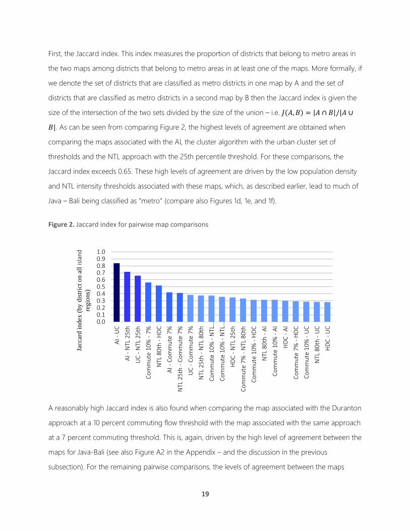
Figure 2 presents values of the Jaccard index for pairwise comparisons of the “metro maps” generated

by the different approaches. And, Figure 3 provides a visualization of the level of agreement between

the different approaches for four selected metro areas – namely, Jakarta, Surabaya, Denpasar, and

Makassar.

19

First, the Jaccard index. This index measures the proportion of districts that belong to metro areas in

the two maps among districts that belong to metro areas in at least one of the maps. More formally, if

we denote the set of districts that are classified as metro districts in one map by A and the set of

districts that are classified as metro districts in a second map by B then the Jaccard index is given the

size of the intersection of the two sets divided by the size of the union – i.e. 𝐽(𝐴, 𝐵) = |𝐴 ∩ 𝐵|/|𝐴 ∪

𝐵|. As can be seen from comparing Figure 2, the highest levels of agreement are obtained when

comparing the maps associated with the AI, the cluster algorithm with the urban cluster set of

thresholds and the NTL approach with the 25th percentile threshold. For these comparisons, the

Jaccard index exceeds 0.65. These high levels of agreement are driven by the low population density

and NTL intensity thresholds associated with these maps, which, as described earlier, lead to much of

Java – Bali being classified as “metro” (compare also Figures 1d, 1e, and 1f).

Figure 2. Jaccard index for pairwise map comparisons

A reasonably high Jaccard index is also found when comparing the map associated with the Duranton

approach at a 10 percent commuting flow threshold with the map associated with the same approach

at a 7 percent commuting threshold. This is, again, driven by the high level of agreement between the

maps for Java-Bali (see also Figure A2 in the Appendix – and the discussion in the previous

subsection). For the remaining pairwise comparisons, the levels of agreement between the maps

0.00.10.20.30.40.50.60.70.80.91.0

AI -

UC

AI -

NTL

25

th

UC

- N

TL 2

5th

Co

mm

ute

10

% -

7%

NTL

80

th -

HD

C

AI -

Co

mm

ute

7%

NTL

25

th -

Co

mm

ute

7%

UC

- C

om

mu

te 7

%

NTL

25

th -

NTL

80

th

Co

mm

ute

10

% -

NTL

…

Co

mm

ute

10

% -

NTL

…

HD

C -

NTL

25

th

Co

mm

ute

7%

- N

TL 8

0th

Co

mm

ute

10

% -

HD

C

NTL

80

th -

AI

Co

mm

ute

10

% -

AI

HD

C -

AI

Co

mm

ute

7%

- H

DC

Co

mm

ute

10

% -

UC

NTL

80

th -

UC

HD

C -

UC

Jacc

ard

ind

ex (

by d

istr

ict

on a

ll is

lan

dre

gio

ns)

20

associated with different approaches and thresholds are much lower. This is generally simply so

because these comparisons involve comparing one map with a strict set of thresholds, generating

only few metro districts, with another map that has a much more relaxed set of thresholds, generating

many metro districts.

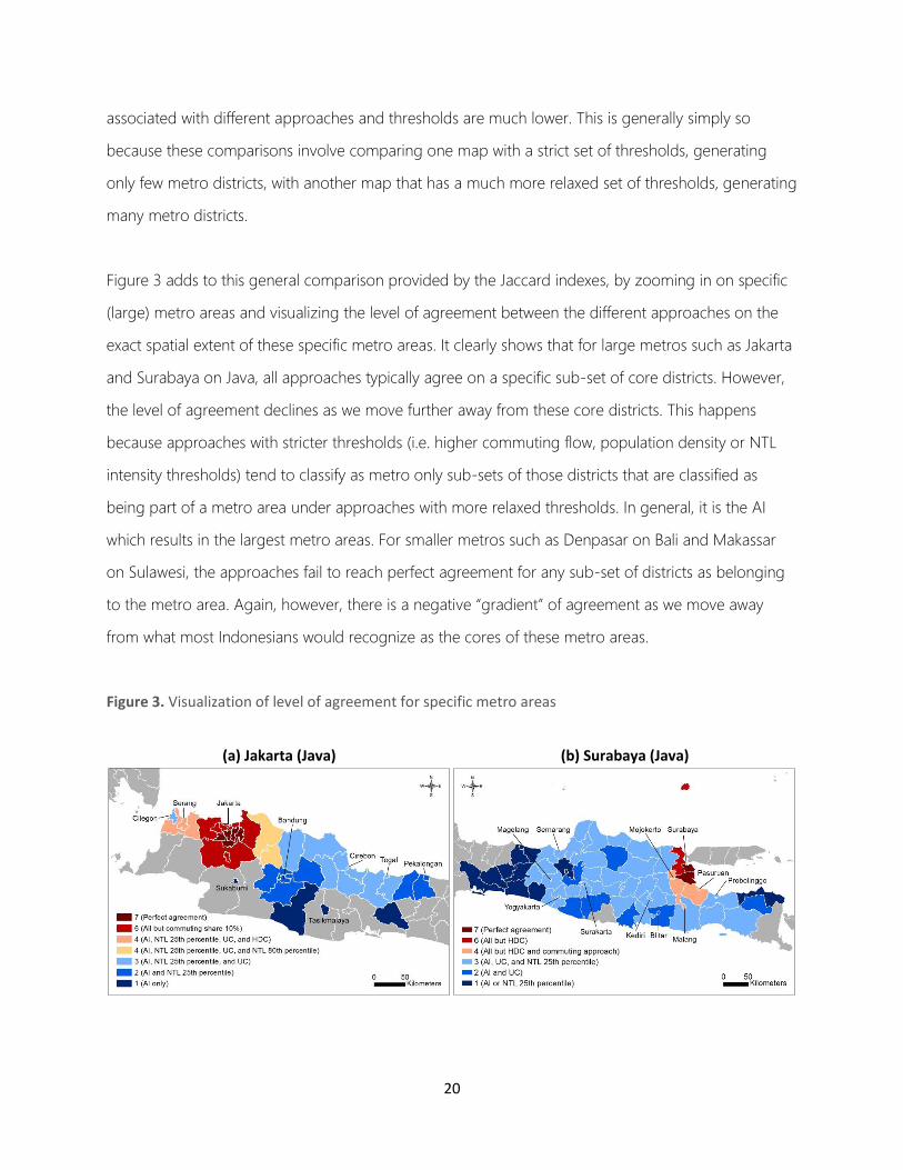
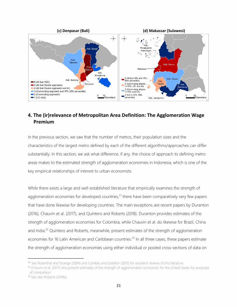
Figure 3 adds to this general comparison provided by the Jaccard indexes, by zooming in on specific

(large) metro areas and visualizing the level of agreement between the different approaches on the

exact spatial extent of these specific metro areas. It clearly shows that for large metros such as Jakarta

and Surabaya on Java, all approaches typically agree on a specific sub-set of core districts. However,

the level of agreement declines as we move further away from these core districts. This happens

because approaches with stricter thresholds (i.e. higher commuting flow, population density or NTL

intensity thresholds) tend to classify as metro only sub-sets of those districts that are classified as

being part of a metro area under approaches with more relaxed thresholds. In general, it is the AI

which results in the largest metro areas. For smaller metros such as Denpasar on Bali and Makassar

on Sulawesi, the approaches fail to reach perfect agreement for any sub-set of districts as belonging

to the metro area. Again, however, there is a negative “gradient” of agreement as we move away

from what most Indonesians would recognize as the cores of these metro areas.

Figure 3. Visualization of level of agreement for specific metro areas

(a) Jakarta (Java) (b) Surabaya (Java)

21

(c) Denpasar (Bali) (d) Makassar (Sulawesi)

4. The (ir)relevance of Metropolitan Area Definition: The Agglomeration Wage Premium

In the previous section, we saw that the number of metros, their population sizes and the

characteristics of the largest metro defined by each of the different algorithms/approaches can differ

substantially. In this section, we ask what difference, if any, the choice of approach to defining metro

areas makes to the estimated strength of agglomeration economies in Indonesia, which is one of the

key empirical relationships of interest to urban economists.

While there exists a large and well-established literature that empirically examines the strength of

agglomeration economies for developed countries,21 there have been comparatively very few papers

that have done likewise for developing countries. The main exceptions are recent papers by Duranton

(2016), Chauvin et al. (2017), and Quintero and Roberts (2018). Duranton provides estimates of the

strength of agglomeration economies for Colombia, while Chauvin et al. do likewise for Brazil, China

and India.22 Quintero and Roberts, meanwhile, present estimates of the strength of agglomeration

economies for 16 Latin American and Caribbean countries.23 In all three cases, these papers estimate

the strength of agglomeration economies using either individual or pooled cross-sections of data on

21 See Rosenthal and Strange (2004) and Combes and Gobillon (2015) for excellent reviews of this literature. 22 Chauvin et al. (2017) also present estimates of the strength of agglomeration economies for the United States for purposes

of comparison. 23 See also Roberts (2018a).

22

workers drawn from either household or labor force surveys. They estimate the strength of

agglomeration economies by regressing a worker’s nominal wage on a measure of either the size or

density of the city in which the worker lives while controlling for observable characteristics of the

worker, including, most notably, the worker’s level of education and workforce experience, as proxied

by the worker’s age.

In what follows below, we follow a similar approach to Duranton (2016), Chauvin et al. (2017) and

Quintero and Roberts (2018) in estimating the strength of agglomeration economies for Indonesia.24

Hence, we draw on micro-data for Indonesian workers from the same survey – SAKERNAS – that we

used to measure commuting flows, to estimate the size of the agglomeration wage premium in a

simple cross-sectional regression framework.25 Importantly, in doing so, we estimate the size of this

premium based on each of the different approaches – Duranton’s algorithm, the AI, the two cluster

algorithms, and the NTL approach – to defining metro areas.

4.1. Empirical Framework

4.1.1. Estimation Strategy

Similar to previous papers for other countries (Duranton, 2016; Chauvin et al., 2017; Quintero and

Roberts, 2018), we identify the strength of Indonesia’s agglomeration wage premium, using the

following basic regression:

ln 𝑤𝑖𝑜𝑗𝑑 = 𝛼𝑗 + 𝛼𝑜 + 𝑿𝒊𝜸𝟏 + 𝑿𝒅𝜸𝟐 + 𝛽 ln 𝑆𝑑𝑚 + 𝜀𝑖𝑜𝑗𝑑 [1]

24 We do not attempt to distinguish between the possible different underlying sources of agglomeration economies. These

sources include the various matching, sharing and learning mechanisms and are discussed in detail by e.g., Duranton and

Puga (2004). 25 Specifically, we use data from the August 2014 round of SAKERNAS. This data is representative for Indonesian districts.

This cross-sectional framework leaves us unable to control for sorting of workers based on time-invariant unobservable

characteristics as their ability (as distinct from their level of education) and motivation. In this sense, we fall short of the

standards of what researchers have been able to achieve in terms of the identification of agglomeration effects for

countries such as the United States (Glaeser and Mare, 2001), France (Combes et al., 2008), or Spain (De la Roca and Puga,

2017) where detailed panel data sets allow the researcher to control for time-invariant unobservable characteristics of

workers.

23

where our dependent variable ln 𝑤𝑜𝑗𝑑𝑖 denotes the hourly nominal wage of individual i, working in

occupation o, in industry j that is in district d.26 It is important to note that d denotes the district where

the job, and not necessarily the worker is located. 𝛼𝑗 denotes a full set of 186 3-digit industry

dummies (with industries as defined in the 2000 Indonesian Standard Industrial Classification, KBLI

2000), and 𝛼𝑜 a full set of 241 occupation dummies (with occupations as defined in the 1982

Indonesian Classification of Occupations, KJI 1982). 𝑿𝒊 denotes a vector of individual worker

characteristics that we can control for in our regressions. Specifically, we control for a worker’s age

and age2, which can (among others) be considered as an (imperfect) measure of his/her overall

workforce experience. We do not have information on the latter, but we always include a worker’s

experience on his/her current job and its square, which is measured as the number of years he/she

has been working on the job, as well as a dummy variable indicating whether he/she ever held a job

before his/her current job. Next, we control for a worker’s highest completed level of education,27 as

well as two dummy variables indicating whether he/she completed at least one, respectively two,

additional formal training courses for which he/she got a certificate. Finally, we include a dummy

variable indicating whether a worker is an “own account worker” or an employee.28 𝑿𝒅 is a set of

dummy variables for the 8 main Indonesian islands (groups) 29 that the district is located on, and 𝜀𝑖𝑜𝑗𝑑

captures all other unobserved nominal wage determinants.

Finally, 𝑆𝑑𝑚 denotes our main independent variable of interest. In our main specification, we follow De

la Roca and Puga (2017) in the specification of this variable. For all districts that belong to a metro

area, it is defined as “the number of people living within 10 km of the average person in the

26 SAKERNAS reports monthly income for sampled individuals. Based on this, and a person’s reported total working hours

during the last week, we calculate his/her hourly wage as: (monthly income / (365/12)) (7/hours worked last week).

SAKERNAS reports both monthly income earned in cash as well as in goods. In all results reported here, we use total

monthly income, i.e. total monthly income in cash and in goods combined. All our findings are robust to using only total

monthly income in cash (see e.g. Table A8 in Appendix A). This is not that surprising as the share of income earned in cash

is 0.981 (1.0) for the average (median) worker. Only for less than 0.75 percent of workers does non-cash income make-up

more than 50 percent of their total income. 27 SAKERNAS indicates a worker’s highest level of completed education in one of 13 different categories of (completed)

education. From lowest to highest level of education, these categories are: no schooling, incomplete primary school,

primary school, package A, general junior high school, vocational junior high school, package B, general senior high school,

vocational senior high school, package C, diploma I/II, diploma III, div/S1, and S2/S3 (university). 28 In our main sample, which we define below, the share of “own account workers” is about 30 percent. Our results are

robust to only considering employees in our regressions. See e.g. Table A7 in Appendix A. 29 These islands (groups) are: Bali, Java, Kalimantan, Maluku, Nusa Tenggara, Papua, Sulawesi, and Sumatera.

24

metropolitan area, m, to which district, d, belongs”, i.e. it takes the same value for all districts

belonging to the same metro area. For all districts that do not belong to a metro area, it is defined as

“the number of people living within 10 km of the average person in the district, d”. Crucially, this

variable varies depending on the algorithm/approach used to define metro areas. We use this

variable instead of a simpler density measure, as it is (see De la Roca and Puga, 2017, p.112) better

able to deal with the noise introduced by urban boundaries that vary across urban areas in their

tightness around built-up areas. We calculate this variable using the same Landscan-2012 gridded

population data that we used to define metro areas using the AI and cluster algorithms (see Section

3.1 above).

In extensions, we also use four other independent variables at the same “ 𝑑𝑚” level as our main city size

variable. First, we obtain the total urban population of each metro area / district from the 2014

Indonesian household survey (Survei Sosial Ekonomi, SUSENAS). Our main city size variable is

essentially a weighted density measure. Using total urban population instead we can assess how

sensitive our results are to the use of a simple overall population size measure. Second, we

constructed two other agglomeration variables from the information in SAKERNAS that measure: (i)

the sectoral specialization of the metro area/district, i.e. the share of a metro’s total employment in

the same sector as the worker him/herself; and (ii) the share of skilled workers in a metro/district’s

total employment, where we define skilled workers as those that have completed general senior high

school or higher. Note that, similar to our main size variable, these two variables, as well as the earlier

discussed “total urban population measure” are defined at the district level for all districts that are not

part of a metro area. Finally, we have calculated each district’s market access that captures a district’s

accessibility to the markets of all other districts within Indonesia taking estimated travel times into

account.30 Taking a metro/district’s sectoral specialization, share of skilled workers and access to other

30 Following, for example, Jedwab and Storeygard (2015), Blankespoor et al. (2017) and Berg et al. (2018), we measure market

access as 𝑀𝐴𝑖 = ∑ 𝑃𝑗𝜏𝑖𝑗−𝜃

𝑗≠𝑖 where 𝑀𝐴𝑖 is a district i’s level of market access, 𝑃𝑗 is the population of district j, and 𝜏𝑖,𝑗 is the

estimated road travel time between districts i and j. Population data is from the 2014 round of SUSENAS. To estimate road

travel time, we construct a road dataset by transferring the 2014 road categories on a paper map published by NELLES to a

geo-referenced network-enabled road dataset (DeLorme) and assume uniform travel time speeds by road category

identical to those assumed by Jedwab and Storeygard (2015) and Berg et al. (2018): expressway 105km/h, principal highway

100km/h, highway 90km/h, secondary road 75km/h, track 50km/h, 6 km/h for the unknown category and 5 km/h in the

absence of a road. For the elasticity of trade, θ, we assume 3.8 following Donaldson (2018).

25

districts’ markets into account, we can assess to what extent our findings are sensitive to taking explicit

account of alternative explanations for agglomeration economies.

In all our regressions, β is our main coefficient of interest. It measures the size of Indonesia’s

agglomeration wage premium. This coefficient is of interest in and of itself, but for the purposes of

this paper, we are particularly interested in seeing how the estimated size (and significance) of β

depends on the approach used to define metro areas. In establishing its significance, it is important to

note that we always cluster our standard errors at the metro or district level (depending on whether a

district belongs to a metro area or not), i.e. at the same level at which our main independent variable

of interest varies.

We estimate equation (1) using ordinary least squares (OLS) regression, so that we can interpret the

estimated β as a consistent estimate of Indonesia’s agglomeration wage premium under the

assumption that 𝜀𝑖𝑜𝑗𝑑 is uncorrelated with the included independent variables in the regression. But,

in an attempt to deal with the possible endogeneity of the metro/urban size measure (which, if

present, would clearly violate this assumption), we also employ a Two-stage Least Squares (2SLS)

regression strategy inspired by De la Roca and Puga (2017), Combes et al. (2010), and Saiz (2010),

where in the first stage, we instrument our size measure with several geographic and climate variables

that, historically, (may) have constrained urban development, but that, today, are unlikely to have an

important influence on workers’ wages. Hence, we use a district’s elevation, ruggedness, temperature

(both its monthly average as well as its standard deviation over the year) and rainfall (both total

monthly rainfall as well as its standard deviation over the year) as instruments.31 These variables are

31 We derived our temperature and rainfall measures from 2013 data produced by the University of East Anglia’s Climate

Research Unit (https://crudata.uea.ac.uk/cru/data/hrg/). Meanwhile, we derived out elevation and ruggedness variables

using data that was originally generated by NASA's Shuttle Radar Topography Mission (SRTM). Terrain ruggedness at the

central point of a grid cell is defined as the mean of the absolute differences in elevation of the central point between the

central grid cell and its eight adjacent grid cells, i.e., grid cells in the north, northeast, east, southeast, south, southwest,

west, and northwest of the central grid cell. That is, 𝑇𝑅𝐼𝑖 = ∑ |𝐸𝑖 − 𝐸𝑗|8𝑗=1 8⁄ , where TRIi denotes the ruggedness in the

central grid cell i, Ei and Ej represent the values of elevation in the central grid cell i and neighboring grid cell j, respectively

(Wilson et al., 2007). Using our elevation data, we ran the TRI command from a Python library (GDAL:

https://docs.qgis.org/2.8/en/docs/user_manual/processing_algs/gdalogr/gdal_analysis.html) and generated a single-band

output raster with the index values. The resultant raster was subsequently used as an input value layer for the zonal

statistics to obtain the mean terrain ruggedness for Indonesian district.

26

either related to a location’s agricultural potential and/or the constraints its geography poses on

urban expansion (ruggedness, elevation). Especially when focusing on the urban workers in our

sample only (see the next sub-section), these instruments should plausibly satisfy the exclusion

restriction.

4.1.2. Main Sample

In estimating equation (1), we follow De la Roca and Puga (2017) as closely as possible, and restrict

attention to working age (15 - 64) males that report a non-zero income in the August 2014 round of

SAKERNAS. This initial sample consists of 116,156 workers. Next, we further exclude workers employed

in agriculture, forestry, livestock and fishing, mining and quarrying, public administration and defense,

education, health and social work. These activities are typically rural or much more controlled /

regulated by the national and local governments in Indonesia. Also, we only focus on workers who

have worked at least 32 hours (four working days) during the last week. These restrictions reduce the

sample to 56,577 workers. In several robustness checks to these choices, we also show results when

extending the sample to females; workers who have worked at least 24 hours (3 working days) in the

previous week; workers in public administration and defense, education, health and social work;

and/or non-production occupations in agriculture, forestry, livestock, fishing and mining and

quarrying. We also perform robustness checks based on restricting the sample to employees or prime

age (25-54) males only, or measuring the hourly wage using cash income only.

4.2. Baseline Results

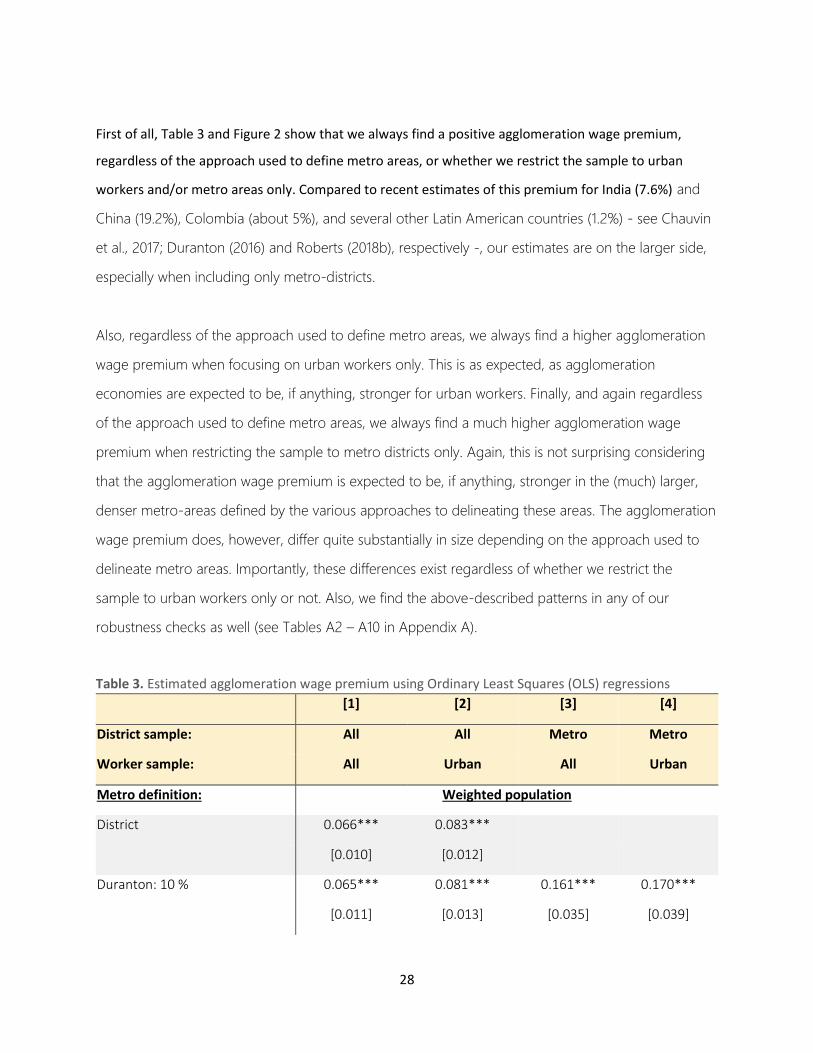
Table 3 and Figure 2 show our main results using De la Roca and Puga’s (2017) preferred measure of

metro/urban size as our main independent variable of interest – i.e. the number of people within 10 km

of the average person in the metro area or district. Table 3, as well as Tables A1 – A10 in Appendix A

that contain various robustness check to our main specification, show the estimated agglomeration

wage premia when relying on seven different ways to define Indonesia’s metro areas – namely,

Duranton’s algorithm based on commuting flow thresholds of 10 percent and 7 percent; the AI; the

cluster algorithm using both the UC (i.e. �̅�𝐷 = 300 people per km2; �̅�𝑃 = 5,000) and the HDC (�̅�𝐷 =

1,500 people per km2; �̅�𝑃 = 50,000) sets of thresholds; and the NTL approach using the 25th and 80th

27

percentile thresholds.32 We focus on these seven based on our discussion in Section 3.3. Besides this,

we also show results when using a “naïve” metro area definition, which simply takes each Indonesian

administrative district as its own metro area. Figure 2 complements these results by plotting the

estimated agglomeration wage premia for metro area definitions calculated using all the different

thresholds for Duranton’s algorithm and the NTL approach that were analyzed in Section 3.3.

For each of these definitions, we show results when estimating equation (1) on four different samples.

These samples become ever stricter in terms of what we consider as cities in our sample. In column [1],

we include all districts and all workers (i.e., both urban and rural) in the sample. As discussed before,

metro districts get assigned the relevant population size measure of the entire metro area that they

belong to, and non-metro districts simply the relevant population size measure of their own district. In

column [2], we again include all districts but restrict the sample to “urban workers” only. The SAKERNAS

classifies each worker as living in an urban or rural area.33 If anything, we expect the agglomeration

premium to be prevalent primarily in an urban context.34.In column [3], we drop non-metro districts and

only consider those districts that belong to a metro area. In these columns, however, we do include

both urban and rural workers. Effectively, we hereby focus entirely on the variation in the size of the

metro areas defined by each of the different approaches discussed in Sections 2 and 3. Finally, in

columns [4], we focus on the urban workers in metro-districts only.35

32 All tables and figures in this section, as well as the tables showing various robustness checks to our main results (see

Appendix A), only report the estimated agglomeration wage premium, β in equation (1). All regressions always include the

full set of controls discussed in Section 4.1.1. Table A1 in Appendix A shows the estimated effect of the various worker

characteristics that we include as controls. They all have the expected impact on nominal wages. These coefficients are very

stable and do not vary with the metro definition used, nor do they change substantially across the various robustness

checks we perform. 33 This classification is based on a composite scoring system which assesses Indonesian villages as either urban or rural based

on their possession of certain “urban characteristics” (BPS Regulation 37/2010). The urban characteristics assessed are: (i)

population density; (ii) the structure of the local economy (specifically, the share of agricultural households); (iii) the

percentage of households with certain types of infrastructure (i.e. electricity and telephone networks); and (iv) the

availability of urban facilities (those considered are schools, hospitals, a market, shops, a cinema, and, finally, recreational

facilities such as a hotel, a salon, a billiard hall, a disco-tec or a massage parlor). Each sub-national administrative unit in

Indonesia at the 4th level (i.e. each “village”) is assigned a score from 1 to 8 for (i) and (ii), respectively, while scoring 1 or 0

for each of eight infrastructure/urban facilities in (iii) and (iv) depending on the availability within a certain distance. If a

village’s total score is 10 or higher, it is classified as urban; and rural, otherwise. 34 Alternatively, we restrict the sample to those districts designated as “Kota”, or city. Districts are either coded as “Kota”, city,

or as “Kabupaten”, village. Results, which are available on request, are very similar to those where we focus on “urban

workers.” 35 When simply defining our population size measures for each separate district, we do not report results in columns [3] –

[4]. These results would simply be identical to those shown in columns [1] – [2].

28

First of all, Table 3 and Figure 2 show that we always find a positive agglomeration wage premium,

regardless of the approach used to define metro areas, or whether we restrict the sample to urban

workers and/or metro areas only. Compared to recent estimates of this premium for India (7.6%) and

China (19.2%), Colombia (about 5%), and several other Latin American countries (1.2%) - see Chauvin

et al., 2017; Duranton (2016) and Roberts (2018b), respectively -, our estimates are on the larger side,

especially when including only metro-districts.

Also, regardless of the approach used to define metro areas, we always find a higher agglomeration

wage premium when focusing on urban workers only. This is as expected, as agglomeration

economies are expected to be, if anything, stronger for urban workers. Finally, and again regardless

of the approach used to define metro areas, we always find a much higher agglomeration wage

premium when restricting the sample to metro districts only. Again, this is not surprising considering

that the agglomeration wage premium is expected to be, if anything, stronger in the (much) larger,

denser metro-areas defined by the various approaches to delineating these areas. The agglomeration

wage premium does, however, differ quite substantially in size depending on the approach used to

delineate metro areas. Importantly, these differences exist regardless of whether we restrict the

sample to urban workers only or not. Also, we find the above-described patterns in any of our

robustness checks as well (see Tables A2 – A10 in Appendix A).

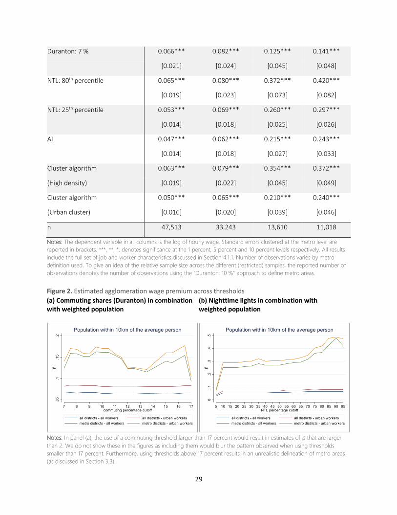
Table 3. Estimated agglomeration wage premium using Ordinary Least Squares (OLS) regressions

[1] [2] [3] [4]

District sample: All All Metro Metro

Worker sample: All Urban All Urban

Metro definition: Weighted population

District 0.066*** 0.083***

[0.010] [0.012]

Duranton: 10 % 0.065*** 0.081*** 0.161*** 0.170***

[0.011] [0.013] [0.035] [0.039]

29

Duranton: 7 % 0.066*** 0.082*** 0.125*** 0.141***

[0.021] [0.024] [0.045] [0.048]

NTL: 80th percentile 0.065*** 0.080*** 0.372*** 0.420***

[0.019] [0.023] [0.073] [0.082]

NTL: 25th percentile 0.053*** 0.069*** 0.260*** 0.297***

[0.014] [0.018] [0.025] [0.026]

AI 0.047*** 0.062*** 0.215*** 0.243***

[0.014] [0.018] [0.027] [0.033]

Cluster algorithm 0.063*** 0.079*** 0.354*** 0.372***

(High density) [0.019] [0.022] [0.045] [0.049]

Cluster algorithm 0.050*** 0.065*** 0.210*** 0.240***

(Urban cluster) [0.016] [0.020] [0.039] [0.046]

n 47,513 33,243 13,610 11,018

Notes: The dependent variable in all columns is the log of hourly wage. Standard errors clustered at the metro level are

reported in brackets. ***, **, *, denotes significance at the 1 percent, 5 percent and 10 percent levels respectively. All results

include the full set of job and worker characteristics discussed in Section 4.1.1. Number of observations varies by metro

definition used. To give an idea of the relative sample size across the different (restricted) samples, the reported number of

observations denotes the number of observations using the “Duranton: 10 %” approach to define metro areas.

Figure 2. Estimated agglomeration wage premium across thresholds

(a) Commuting shares (Duranton) in combination with weighted population

(b) Nighttime lights in combination with weighted population

Notes: In panel (a), the use of a commuting threshold larger than 17 percent would result in estimates of β that are larger

than 2. We do not show these in the figures as including them would blur the pattern observed when using thresholds

smaller than 17 percent. Furthermore, using thresholds above 17 percent results in an unrealistic delineation of metro areas

(as discussed in Section 3.3).

30

4.2.1 Including All Districts in the Sample

Interestingly, the differences in the estimated agglomeration wage premium, i.e. the estimate of ,

across approaches and thresholds are smallest when including all districts in the sample (see columns

[1] – [2] in Table 3). Furthermore, the estimated agglomeration premium is always smaller than that

estimated using a naïve district-based metro area definition (i.e. where we simply define each district

as a metro). The largest differences can be found across the different approaches to delineating

metro areas. Within approaches, i.e. for the different commuting share or NTL thresholds used, results

are very stable when including all districts in the sample (see the blue and red lines in Figure 2). The

estimated agglomeration wage premium is smallest when using the AI or the cluster algorithm with

the UC set of thresholds to define metro areas, followed by the NTL approach using below median

intensity (up to the 50th percentile). Using Duranton’s algorithm with a commuting threshold lower

than 17 percent, the NTL approach using above median percentile of intensity, and the cluster

algorithm with the HDC thresholds to delineate metro areas all give us estimated agglomeration

wage premia that are only slightly smaller than that obtained using a naïve district-based metro area

definition.

Of course, it may not be that surprising that the estimated agglomeration wage premia using the

different approaches to delineating metro areas is not that different from that obtained when simply

taking each district for a metro area. The number of metro-districts is at most 135 (when using the

cluster algorithm with the UC thresholds) and can be as small as 38 (when using the cluster algorithm

with the HDC thresholds). The total number of districts in our sample is 497, so that, at most, 27

percent of all districts get assigned a different “city size variable” than when using the naïve district-

based metro area definition. Moreover, for the metro-districts, a district’s own “city size variable” is

typically not very different from that defined for the entire metro area that the district is part of. Table

4 below illustrates this by reporting the correlation between the “city size variable” at the district level

and that at each of the seven main metro area levels for which we also show results in Table 3. It

shows these correlations for each of the two main city size variables (i.e. weighted population and

31

urban population) used in our analysis, as well as when including all, or only urban, workers in the

sample.

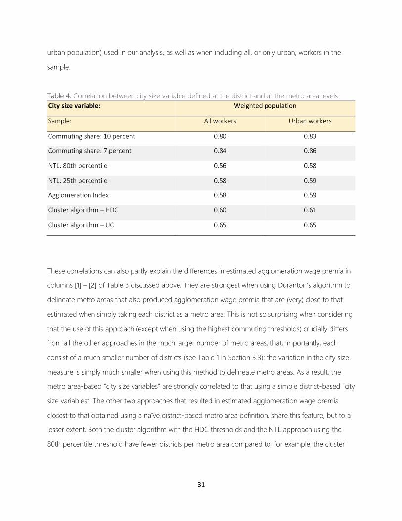
Table 4. Correlation between city size variable defined at the district and at the metro area levels

City size variable: Weighted population

Sample: All workers Urban workers

Commuting share: 10 percent 0.80 0.83

Commuting share: 7 percent 0.84 0.86

NTL: 80th percentile 0.56 0.58

NTL: 25th percentile 0.58 0.59

Agglomeration Index 0.58 0.59

Cluster algorithm – HDC 0.60 0.61

Cluster algorithm – UC 0.65 0.65

These correlations can also partly explain the differences in estimated agglomeration wage premia in

columns [1] – [2] of Table 3 discussed above. They are strongest when using Duranton’s algorithm to

delineate metro areas that also produced agglomeration wage premia that are (very) close to that

estimated when simply taking each district as a metro area. This is not so surprising when considering

that the use of this approach (except when using the highest commuting thresholds) crucially differs

from all the other approaches in the much larger number of metro areas, that, importantly, each

consist of a much smaller number of districts (see Table 1 in Section 3.3): the variation in the city size

measure is simply much smaller when using this method to delineate metro areas. As a result, the

metro area-based “city size variables” are strongly correlated to that using a simple district-based “city

size variables”. The other two approaches that resulted in estimated agglomeration wage premia

closest to that obtained using a naïve district-based metro area definition, share this feature, but to a

lesser extent. Both the cluster algorithm with the HDC thresholds and the NTL approach using the

80th percentile threshold have fewer districts per metro area compared to, for example, the cluster

32

algorithm with the UC thresholds or the AI (but far fewer metro areas overall compared to Duranton’s

algorithm using a 10 percent or 7 percent commuting threshold).

4.2.2 Including only Metro Districts

We observe much more variation in the estimated agglomeration wage premium when we restrict the

sample to metro districts only. This can be explained by the fact that now we do not only change the

“city size variable” for each of the metro districts from its own to that of the metro area it is part of,

but we now also run our regressions on often very different samples. These samples range from all

workers in the 138 metro districts based on the UC algorithm, to those in only about 40 metro districts

based on the HDC algorithm or the 80th percentile of NTL intensity (and even fewer when

considering some of the results in Figure 2).

Interestingly, the variation in the estimated agglomeration wage premium appears to be (at least

partly) related to both the total number of metro districts identified by the approach used, as well as

the average number of metro districts per metro area. It is largest when using either the cluster

algorithm with the HDC thresholds or the 80th percentile of NTL intensity. These are exactly the

approaches resulting in the fewest metro districts (see Table 1 and Figure 1 in Section 3.3). The cluster

algorithm with the UC thresholds and the AI, as well as the NTL approach using a 25th percentile

threshold identify many more districts as metro-districts, and result in a smaller estimated

agglomeration wage premium.36 However, the number of metro districts per metro area identified

also appears to play an important role in explaining the variation in results shown in columns [3] and

[4] of Table 3: the agglomeration wage premium is smallest when using Duranton’s algorithm, which

is characterized by fewer districts per metro area than any of the other approaches.

4.3. Accounting for Potential Endogeneity of Our Main City Size Variables

36 When using the NTL approach to delineate metro areas, the estimated agglomeration wage premium also decreases with

the number of metro districts identified (i.e. it increases with the NTL intensity threshold). See Figure 2(b).

33

All results discussed so far were obtained by estimating equation (1) using OLS regressions. This

section aims to mitigate any remaining endogeneity concerns that one may have regarding these

results. These concerns include the omission of other important determinants of nominal wages that

are correlated with any of the included regressors in equation (1), or reverse causality issues, i.e.

higher nominal wages attracting workers/people instead of larger/denser cities generating

agglomeration rents.

To do this, we instead estimate equation (1) using 2SLS, where, in the first stage, we instrument our

city size measure with several geographic and climate variables that, historically, (may) have

constrained urban development, but that, today, are unlikely to have an important influence on

workers’ wages. These variables are either related to a location’s agricultural potential (temperature,

rainfall) and/or the constraints its geography poses on urban expansion (ruggedness, elevation) - see

the discussion at the end of Section 4.2.1 for the exact variables used. Especially when focusing on the

particular (urban) workers in our sample (see the next subsection), these instruments should plausibly

satisfy the exclusion restriction.

Table 5 below shows the resulting estimated agglomeration wage premia using the same approaches

to delineating metro areas for which we showed results in Table 3. Figure A3 in Appendix A further

complements Table 5 by showing the estimated agglomeration wage premiums across different

thresholds both for Duranton’s algorithm (panels (a) and (b)) and for the NTL approach (panels (c)

and (d)) to delineating metro areas. The estimated agglomeration wage premium is typically (much)

larger when using this IV-approach.37 However, most important for our purposes, our main findings

as to how this estimated wage premium differs depending on the approach used to define

metropolitan areas, hold up.

Table 5. Estimated agglomeration wage premium using 2-Stage Least Squares Regressions

[1] [2] [3] [4]

District sample: All All Metro Metro

37 A potential explanation for OLS underestimating the agglomeration wage premium would be sorting on unobservables

that are negatively (positively) related to wages and positively (negatively) to urban density.

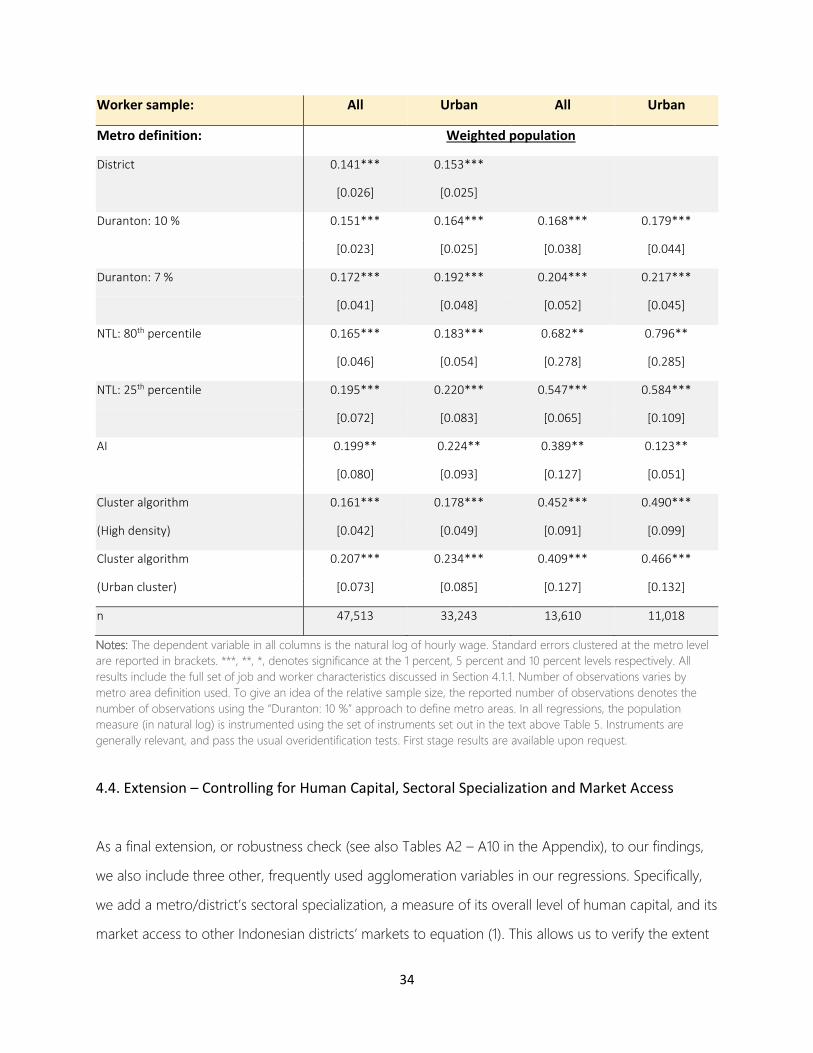
34

Worker sample: All Urban All Urban

Metro definition: Weighted population

District 0.141*** 0.153***

[0.026] [0.025]

Duranton: 10 % 0.151*** 0.164*** 0.168*** 0.179***

[0.023] [0.025] [0.038] [0.044]

Duranton: 7 % 0.172*** 0.192*** 0.204*** 0.217***

[0.041] [0.048] [0.052] [0.045]

NTL: 80th percentile 0.165*** 0.183*** 0.682** 0.796**

[0.046] [0.054] [0.278] [0.285]

NTL: 25th percentile 0.195*** 0.220*** 0.547*** 0.584***

[0.072] [0.083] [0.065] [0.109]

AI 0.199** 0.224** 0.389** 0.123**

[0.080] [0.093] [0.127] [0.051]

Cluster algorithm 0.161*** 0.178*** 0.452*** 0.490***

(High density) [0.042] [0.049] [0.091] [0.099]

Cluster algorithm 0.207*** 0.234*** 0.409*** 0.466***

(Urban cluster) [0.073] [0.085] [0.127] [0.132]

n 47,513 33,243 13,610 11,018

Notes: The dependent variable in all columns is the natural log of hourly wage. Standard errors clustered at the metro level

are reported in brackets. ***, **, *, denotes significance at the 1 percent, 5 percent and 10 percent levels respectively. All

results include the full set of job and worker characteristics discussed in Section 4.1.1. Number of observations varies by

metro area definition used. To give an idea of the relative sample size, the reported number of observations denotes the

number of observations using the “Duranton: 10 %” approach to define metro areas. In all regressions, the population

measure (in natural log) is instrumented using the set of instruments set out in the text above Table 5. Instruments are

generally relevant, and pass the usual overidentification tests. First stage results are available upon request.

4.4. Extension – Controlling for Human Capital, Sectoral Specialization and Market Access

As a final extension, or robustness check (see also Tables A2 – A10 in the Appendix), to our findings,

we also include three other, frequently used agglomeration variables in our regressions. Specifically,

we add a metro/district’s sectoral specialization, a measure of its overall level of human capital, and its

market access to other Indonesian districts’ markets to equation (1). This allows us to verify the extent

35

to which our findings are sensitive to taking explicit account of these alternative explanations for

agglomeration economies.

Table 6 below shows the resulting estimated agglomeration wage premiums using the same

approaches to delineating metro areas for which we showed results in Table 3.38 Columns [1] – [4]

show that all results for our main city size measure, i.e., the population within 10 km of the average

person in the metro area/district, are close to those we found before. The main difference with our

baseline results in Table 3 is a generally slightly smaller estimated agglomeration wage premium.

Table 6. Estimated agglomeration wage premium using Ordinary Least Squares regressions after controlling for overall human capital, sectoral specialization, and market access

[1] [2] [3] [4]

District sample: All All Metro Metro

Worker sample: All Urban All Urban

Metro definition: Weighted population

District 0.039*** 0.051***

[0.013] [0.017]

Duranton: 10 % 0.036*** 0.045*** 0.156*** 0.164***

[0.013] [0.016] [0.048] [0.054]

Duranton: 7 % 0.034** 0.043** 0.065 0.068

[0.017] [0.021] [0.054] [0.057]

NTL: 80th percentile 0.048** 0.060** 0.308** 0.345***

[0.019] [0.023] [0.095] [0.097]

NTL: 25th percentile 0.046** 0.054** 0.132* 0.154*

[0.018] [0.022] [0.069] [0.073]

AI 0.038** 0.046** 0.128*** 0.123***

[0.018] [0.022] [0.034] [0.033]

38 Results for the three additionally included agglomeration variables are available upon request. Generally, we find that a

district’s market access to other Indonesian districts, if significant, negatively affects nominal wages, and, if significant, a

positive effect of a metro area’s share of skilled people in the workforce, and a mostly insignificant negative effect of a

metro area’s degree of sectoral specialization.

36

Cluster algorithm 0.040** 0.052** 0.337*** 0.364***

(High density) [0.019] [0.023] [0.068] [0.074]

Cluster algorithm 0.039* 0.047* 0.180** 0.206*

(Urban cluster) [0.020] [0.025] [0.082] [0.098]

n 47,513 33,243 13,610 11,018

Notes: The dependent variable in all columns is the natural log of hourly wage. Standard errors clustered at the metro level

are reported in brackets. ***, **, *, denotes significance at the 1 percent, 5 percent and 10 percent levels respectively. All

results include the full set of job and worker characteristics discussed in Section 4.1.1, as well as the share of skilled workers in

the metro area’s workforce, the share of workers in the metro area’s workforce employed in the same sector as the worker

him/herself, as well as the natural log of a district’s market access to all other Indonesian districts. See Section 4.1.1 for a

detailed definition of these variables. The number of observations varies by metro area definition used. To give an idea of

the relative sample size, the reported number of observations denotes the number of observations using the “Duranton:

10 %” approach to define metro areas.

5. Conclusion

While a variety of approaches have been developed in the literature for the delineation of metro

areas, there has been little effort to compare these approaches and to assess how the choice of

approach affects key empirical insights on the forces that determine the productivity and growth of

urban areas. In this paper, we have attempted to fill this gap by focusing on Indonesia. Because

Indonesia has a national labor force survey from which an origin – destination commuting flow matrix

can be derived, this allows the implementation of an algorithm attributable to Duranton (2015b) that

allows for the delineation of metro areas based on these flows. Such an algorithm represents an

example of what most economists would consider a “first best” approach to defining metro areas. We

compare results obtained from Duranton’s algorithm with those obtained using other prominent

“satellite-data based” approaches that have been developed for delineating metro areas in the

absence of commuting flow data. These approaches are the Agglomeration Index, the cluster

algorithm, and the thresholding of nighttime lights data.

Overall, we find that definition matters. This is true both in terms of the basic description of

Indonesia’s urban landscape that the adoption of a given definition gives rise to and the estimated

size of the agglomeration wage premium. A defining feature of Duranton’s algorithm using

commuting flow thresholds of 10 percent and 7 percent is that it generates a relatively large number

37

of metro areas, each of which is typically comprised of a small number of districts. The other “satellite-

data based” approaches tend to generate much smaller numbers of much larger metro areas. Given

the country’s high average population density, both the Agglomeration Index and the cluster

algorithm with the urban cluster set of thresholds even produce results that look implausible for

Indonesia. The cluster algorithm with the high-density cluster set of thresholds and the nighttime

lights approach with a threshold set at the 80th percentile of the distribution of luminosity values

produce descriptions that look more reasonable, but which, nevertheless, differ significantly from

those generated by algorithm based on O-D commuting flows. Similarly, the estimated

agglomeration wage premium, while always positive, sizeable and significant, varies substantially with

the exact approach used to define metro areas. This is especially true, when estimating this premium

based on districts belonging to the metro areas defined by the different algorithms only.

If a commuting flow based approach to delineating metro areas is indeed to be preferred, one

important implication of our findings is that one should not necessarily assume that, in the absence of

commuting flow data, alternative approaches to defining metro areas should be preferred over the

simple use of sub-national administrative units as defined by national statistical offices. Hence, the

biases that result from choosing the “wrong” approach to delineating metro areas may well be worse

than those associated with the simple use of sub-national admin units in the estimation of the

agglomeration wage premium and other key empirical relationships in urban economics.

38

References

Berg, C. N., B. Blankespoor, Li, and H. Selod. 2017. Global travel time to major cities, circa 2010. Unpublished

manuscript under preparation. Washington, D.C.: The World Bank.

Berg, C.N., Blankespoor, B. and Selod, H., 2018. “Roads and rural development in Sub-Saharan Africa.” The

Journal of Development Studies, 1-19.

Blankespoor, B., Bougna, T., Garduno Rivera, R. and Selod, H., 2017. Roads and the geography of economic

activities in Mexico. Policy Research Working Paper 8226.

CAF (Development Bank of Latin America). 2017. Urban Growth and Access to Opportunities: A Challenge for

Latin America. 2017 Report on Economic Development (RED). Caracas.

Chauvin, J. P., E. Glaeser, Y. Ma, and K. Tobio. 2017. “What is different about urbanization in rich and poor

countries? Cities in Brazil, China, India and the United States.” Journal of Urban Economics 98 (C): 17-49.

Combes, P-P., G. Duranton, and L. Gobillon. 2008. “Spatial Wage Disparities: Sorting Matters!” Journal of Urban

Economics 63 (2): 723-42.

Combes, P-P., G. Duranton, L. Gobillon, and S. Roux. 2010. “Estimating Agglomeration Effects with History,

Geology, and Worker Fixed-Effects”, in Glaeser, E. L. (ed.) Agglomeration Economics, Chicago, IL: Chigago

University, 15-65.

Combes, P-P., and L. Gobillon. 2015. “The Empirics of Agglomeration Economies.” In Handbook of Regional and

Urban Economics, Volume 5, edited by G. Duranton, J. V. Henderson, and W. Strange, 247-348. Amsterdam:

Elsevier.

Danko, D.M. 1992. “The digital chart of the world project.” Photogrammetric Engineering & Remote Sensing 58:

1125-1128.

De La Roca, J. and D. Puga. 2017. “Learning by Working in Big Cities.” Review of Economic Studies, 84: 106-142.

Dijkstra, L., and H. Poelman. 2014. “A harmonised definition of cities and rural areas: The new degree of

urbanization.” Regional Working Paper, Directorate-General for Regional and Urban Policy, European

Commission, Brussels.

Doll, C. N. H., ed. 2008. CIESIN Thematic Guide to Night-Time Light Remote Sensing and Its Applications.

Palisades, NY: Center for International Earth Science Information Network of Columbia University.

Donaldson, D. 2018. “Railroads and the Raj: Estimating the impact of transportation infrastructure.” American

Economic Review, in press.

Duranton, G. 2015a. “Growing through cities in developing countries.” The World Bank Research Observer 30 (1):

39-73.

Duranton, G. 2015b. “A Proposal to Delineate Metropolitan Areas in Colombia.” Desarrollo y Sociedad 15: 223-

64.

Duranton, G. 2016. “Agglomeration Effects in Colombia.” Journal of Regional Science 56 (2): 210-38.

Duranton, G., and D. Puga. 2004. “Micro-Foundations of Urban Agglomeration Economies.” In Handbook of

Regional and Urban Economics, Volume 4: Cities and Geography, edited by J. V. Henderson and J.-F. Thisse,

2063-2117. Amsterdam: Elsevier.

Ellis, P., and M. Roberts. 2016. Leveraging Urbanization in South Asia: Managing Spatial Transformation for

Prosperity and Livability. World Bank. Washington, DC: World Bank.

Elvidge, C. D., K. E. Kihn, and E. R. Davis. 1996. “Mapping city lights with nighttime data from the DMSP-OLS

operational linescan system.” Photogrammetric Engineering & Remote Sensing 63: 727-734.

Glaeser, E. L., and J. V. Henderson. 2017. “Urban Economics for the Developing World: An Introduction.” Journal

of Urban Economics, 98: 1-5.

Glaeser, E. L., and D. C. Mare. 2001. “Cities and Skills.” Journal of Labor Economics 19 (2): 316-342.

Henderson, J. V., D. Nigmatulina, and S. Kriticos. 2018. “Measuring Urban Economic Density.” Unpublished,

London School of Economics and Political Science, London.

39

Imhoff, M. L., W. T. Lawrence, D. C. Stutzer, and C. D. Elvidge. 1997. “A Technique for Using Composite

Dmsp/Ols “City Lights” Satellite Data to Map Urban Area.” Remote Sensing of Environment 61 (3): 361-370.

Jedwab, R., and A. Storeygard. 2015. The Heterogeneous Effects of Transportation Investments: Evidence from

sub-Sub-Saharan Africa. mimeo, presented at the GWU/World Bank 3rd Urbanization and Poverty

Reduction Research Conference (February 1, 2016).

Overman, H. G., and A. J. Venables. 2005. “Cities in the developing world.” Center for Economic Performance

Discussion Paper 695, London School of Economics and Political Science, London.

Pinkovskiy, M. L. 2013. “Economic Discont inuit ies at Borders: Evidence from Satellite Data on Lights at Night.”

Unpublished, Massachusetts Institute of Technology, Cambridge, MA.

Quintero, L., and M. Roberts. 2018. “Explaining Spatial Variations in Productivity: Evidence from 16 Latin

American and Caribbean Countries.” Policy Research Working Paper, World Bank, Washington, DC.

Roberts, M. 2018a. “The Empirical Determinants of City Productivity.” In Raising the Bar for Productive Cities in

Latin America and the Caribbean, edited by M.M. Ferreyra and M. Roberts, 89-115. Washington, D.C.: The

World Bank.

Roberts, M. 2018b. “The Many Dimensions of Urbanization and the Productivity of Cities in Latin America and

the Caribbean.” In Raising the Bar for Productive Cities in Latin America and the Caribbean, edited by M.M.

Ferreyra and M. Roberts, 49-85. Washington, D.C.: The World Bank.

Roberts, M., B. Blankespoor, C. Deuskar, and B. Stewart. 2017. “Urbanization and Development. Is Latin America

and the Caribbean Different from the Rest of the World?” Policy Research Working Paper 8019, World Bank,

Washington, DC.

Rosenthal, S. S., and W. C. Strange. 2004. “Evidence on the Nature and Sources of Agglomeration Economies.”

In Handbook of Urban and Regional Economics, Volume 4, edited by J. V. Henderson and J.-F. Thisse, 2119-

71. New York: North Holland.

Rozenfeld, H. D., D. Rybski, X. Gabaix, and H. A. Makse. 2011. “The area and population of cities: New insights

from a different perspective on cities.” American Economic Review 101: 2205-2225.

Saiz, A. 2010. “The Geographic Determinants of Housing Supply”, Quarterly Journal of Economics, 125: 1253-

1296.

Small, C., F. Pozzi, and C. D. Elvidge. 2005. “Spatial Analysis of Global Urban Extent from Dmsp-Ols Night

Lights.” Remote Sensing of Environment 96 (3–4): 277-291.

Sutton, P. C. 2003. “A scale-adjusted measure of "urban sprawl" using nighttime satellite imagery.” Remote

Sensing of Environment 86: 353-363.

Uchida, H., and A. Nelson. 2009. Agglomeration Index: Towards a New Measure of Urban Concentration.

Washington, DC: World Bank.

Wilson, M. F. J., B. O’Connell, C. Brown, J. C. Guinan, and A. J. Grehan. 2007. “Multiscale Terrain Analysis of

Multibeam Bathymetry Data for Habitat Mapping on the Continental Slope.” Marine Geodesy 30: 3-35.

Available from: https://www2.unil.ch/biomapper/Download/Wilson-MarGeo-2007.pdf

World Bank. 2008. World Development Report, 2009: Reshaping economic geography. Washington, DC: World

Bank.

World Bank. 2018. Indonesia Economic Quarterly. September 2018 edition. Forthcoming.

World Bank & IMF. 2013. Global Monitoring Report 2013: Rural-Urban Dynamics and the Millennium

Development Goals. Washington, DC: World Bank.

Zhang, Q., and K. C. Seto. 2011. “Mapping Urbanization Dynamics at Regional and Global Scales Using Multi-

Temporal DMSP/OLS Nighttime Light Data.” Remote Sensing of Environment 115 (9): 2320–29.

Zhou, N., K. Hubacek, and M. Roberts. 2015. “Analysis of Spatial Patterns of Urban Growth across South Asia

Using DMSP-OLS Nighttime Lights Data.” Applied Geography 63: 292-303.

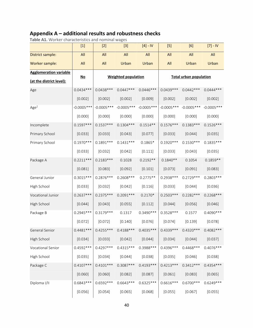
40

Appendix A – additional results and robustness checks Table A1. Worker characteristics and nominal wages

[1] [2] [3] [4] - IV [5] [6] [7] - IV

District sample: All All All All All All All

Worker sample: All All Urban Urban All Urban Urban

Agglomeration variable

(at the district level): No Weighted population Total urban population

Age 0.0434*** 0.0438*** 0.0447*** 0.0446*** 0.0439*** 0.0442*** 0.0444***

[0.002] [0.002] [0.002] [0.009] [0.002] [0.002] [0.002]

Age2 -0.0005*** -0.0005*** -0.0005*** -0.0005*** -0.0005*** -0.0005*** -0.0005***

[0.000] [0.000] [0.000] [0.000] [0.000] [0.000] [0.000]

Incomplete 0.1597*** 0.1537*** 0.1304*** 0.1514** 0.1576*** 0.1383*** 0.1526***

Primary School [0.033] [0.033] [0.043] [0.077] [0.033] [0.044] [0.035]

Primary School 0.1970*** 0.1891*** 0.1431*** 0.1865* 0.1920*** 0.1530*** 0.1835***

[0.033] [0.032] [0.042] [0.111] [0.033] [0.043] [0.035]

Package A 0.2211*** 0.2183*** 0.1028 0.2192** 0.1840** 0.1054 0.1859**

[0.081] [0.083] [0.092] [0.101] [0.073] [0.091] [0.083]

General Junior 0.3015*** 0.2876*** 0.2608*** 0.2775** 0.2938*** 0.2729*** 0.2803***

High School [0.033] [0.032] [0.042] [0.116] [0.033] [0.044] [0.036]

Vocational Junior 0.2637*** 0.2375*** 0.2091*** 0.2170* 0.2503*** 0.2282*** 0.2268***

High School [0.044] [0.043] [0.055] [0.112] [0.044] [0.056] [0.046]

Package B 0.2945*** 0.3179*** 0.1317 0.3490*** 0.3528*** 0.1577 0.4090***

[0.072] [0.072] [0.140] [0.076] [0.074] [0.139] [0.078]

General Senior 0.4481*** 0.4255*** 0.4188*** 0.4035*** 0.4339*** 0.4320*** 0.4082***

High School [0.034] [0.033] [0.042] [0.044] [0.034] [0.044] [0.037]

Vocational Senior 0.4592*** 0.4297*** 0.4315*** 0.3988*** 0.4396*** 0.4468*** 0.4076***

High School [0.035] [0.034] [0.044] [0.038] [0.035] [0.046] [0.038]

Package C 0.4107*** 0.4101*** 0.3087*** 0.4193*** 0.4213*** 0.3412*** 0.4354***

[0.060] [0.060] [0.082] [0.087] [0.061] [0.083] [0.065]

Diploma I/II 0.6843*** 0.6592*** 0.6643*** 0.6325*** 0.6616*** 0.6700*** 0.6249***

[0.056] [0.054] [0.065] [0.068] [0.055] [0.067] [0.055]

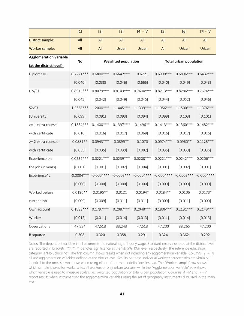
41

[1] [2] [3] [4] - IV [5] [6] [7] - IV

District sample: All All All All All All All

Worker sample: All All Urban Urban All Urban Urban

Agglomeration variable

(at the district level): No Weighted population Total urban population

Diploma III 0.7221*** 0.6800*** 0.6642*** 0.6221 0.6909*** 0.6806*** 0.6432***

[0.040] [0.038] [0.046] [0.665] [0.040] [0.049] [0.043]

Div/S1 0.8515*** 0.8079*** 0.8143*** 0.7604*** 0.8213*** 0.8286*** 0.7674***

[0.045] [0.042] [0.049] [0.045] [0.044] [0.052] [0.046]

S2/S3 1.2358*** 1.2000*** 1.1445*** 1.1339*** 1.1956*** 1.1500*** 1.1376***

(University) [0.099] [0.091] [0.093] [0.094] [0.099] [0.103] [0.101]

>= 1 extra course 0.1334*** 0.1400*** 0.1397*** 0.1496** 0.1413*** 0.1360*** 0.1482***

with certificate [0.016] [0.016] [0.017] [0.069] [0.016] [0.017] [0.016]

>= 2 extra courses 0.0881** 0.0943*** 0.0899** 0.1070 0.0974*** 0.0960** 0.1125***

with certificate [0.035] [0.035] [0.039] [0.082] [0.035] [0.039] [0.036]

Experience on 0.0232*** 0.0221*** 0.0239*** 0.0208*** 0.0221*** 0.0242*** 0.0206***

the job (in years) [0.001] [0.001] [0.002] [0.004] [0.001] [0.002] [0.001]

Experience^2 -0.0004*** -0.0004*** -0.0005*** -0.0004*** -0.0004*** -0.0005*** -0.0004***

[0.000] [0.000] [0.000] [0.000] [0.000] [0.000] [0.000]

Worked before 0.0196** 0.0195** 0.0121 0.0194* 0.0184** 0.0106 0.0173*

current job [0.009] [0.009] [0.011] [0.011] [0.009] [0.011] [0.009]

Own account 0.1583*** 0.1797*** 0.2087*** 0.2048*** 0.1806*** 0.2131*** 0.2143***

Worker [0.012] [0.011] [0.014] [0.013] [0.011] [0.014] [0.013]

Observations 47,554 47,513 33,243 47,513 47,200 33,265 47,200

R-squared 0.308 0.320 0.358 0.291 0.324 0.362 0.292

Notes: The dependent variable in all columns is the natural log of hourly wage. Standard errors clustered at the district level

are reported in brackets. ***, **, *, denotes significance at the 1%, 5%, 10% level, respectively. The reference education

category is “No Schooling”. The first column shows results when not including any agglomeration variable. Columns [2] – [7]

all use agglomeration variables defined at the district level. Results on these individual worker characteristics are virtually

identical to the ones shown above when using either of our metro-definitions instead. The “Worker sample” row shows

which sample is used for workers, i.e., all workers or only urban workers, while the “Agglomeration variable” row shows

which variable is used to measure scales, i.e., weighted population or total urban population. Columns [4]-IV and [7]-IV

report results when instrumenting the agglomeration variables using the set of geography instruments discussed in the main

text.

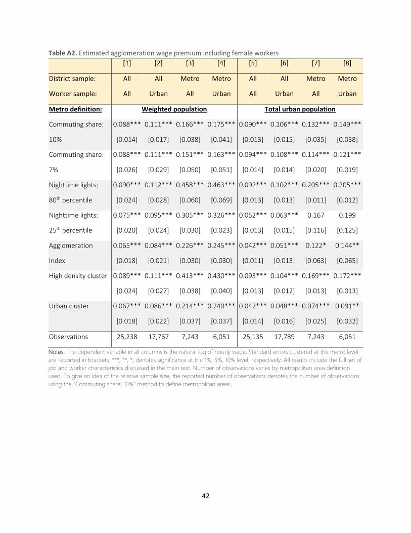
42

Table A2. Estimated agglomeration wage premium including female workers

[1] [2] [3] [4] [5] [6] [7] [8]

District sample: All All Metro Metro All All Metro Metro

Worker sample: All Urban All Urban All Urban All Urban

Metro definition: Weighted population Total urban population

Commuting share: 0.088*** 0.111*** 0.166*** 0.175*** 0.090*** 0.106*** 0.132*** 0.149***

10% [0.014] [0.017] [0.038] [0.041] [0.013] [0.015] [0.035] [0.038]

Commuting share: 0.088*** 0.111*** 0.151*** 0.163*** 0.094*** 0.108*** 0.114*** 0.121***

7% [0.026] [0.029] [0.050] [0.051] [0.014] [0.014] [0.020] [0.019]

Nighttime lights: 0.090*** 0.112*** 0.458*** 0.463*** 0.092*** 0.102*** 0.205*** 0.205***

80th percentile [0.024] [0.028] [0.060] [0.069] [0.013] [0.013] [0.011] [0.012]

Nighttime lights: 0.075*** 0.095*** 0.305*** 0.326*** 0.052*** 0.063*** 0.167 0.199

25th percentile [0.020] [0.024] [0.030] [0.023] [0.013] [0.015] [0.116] [0.125]

Agglomeration 0.065*** 0.084*** 0.226*** 0.245*** 0.042*** 0.051*** 0.122* 0.144**

Index [0.018] [0.021] [0.030] [0.030] [0.011] [0.013] [0.063] [0.065]

High density cluster 0.089*** 0.111*** 0.413*** 0.430*** 0.093*** 0.104*** 0.169*** 0.172***

[0.024] [0.027] [0.038] [0.040] [0.013] [0.012] [0.013] [0.013]

Urban cluster 0.067*** 0.086*** 0.214*** 0.240*** 0.042*** 0.048*** 0.074*** 0.091**

[0.018] [0.022] [0.037] [0.037] [0.014] [0.016] [0.025] [0.032]

Observations 25,238 17,767 7,243 6,051 25,135 17,789 7,243 6,051

Notes: The dependent variable in all columns is the natural log of hourly wage. Standard errors clustered at the metro level

are reported in brackets. ***, **, *, denotes significance at the 1%, 5%, 10% level, respectively. All results include the full set of

job and worker characteristics discussed in the main text. Number of observations varies by metropolitan area definition

used. To give an idea of the relative sample size, the reported number of observations denotes the number of observations

using the “Commuting share: 10%” method to define metropolitan areas.

43

Table A3. Estimated agglomeration wage premium using worker sample of prime-age (25-54) males

[1] [2] [3] [4] [5] [6] [7] [8]

District sample: All All Metro Metro All All Metro Metro

Worker sample: All Urban All Urban All Urban All Urban

Metro definition: Weighted population Total urban population

Commuting share: 0.061*** 0.077*** 0.160*** 0.170*** 0.067*** 0.083*** 0.144*** 0.161***

10% [0.011] [0.013] [0.033] [0.036] [0.011] [0.014] [0.028] [0.031]

Commuting share: 0.061*** 0.077*** 0.125*** 0.141*** 0.072*** 0.086*** 0.102*** 0.114***

7% [0.020] [0.023] [0.043] [0.046] [0.013] [0.014] [0.016] [0.016]

Nighttime lights: 0.061*** 0.076*** 0.349*** 0.391*** 0.073*** 0.085*** 0.165*** 0.182***

80th percentile [0.019] [0.022] [0.073] [0.079] [0.012] [0.013] [0.020] [0.023]

Nighttime lights: 0.049*** 0.064*** 0.262*** 0.298*** 0.046*** 0.057*** 0.168 0.202

25th percentile [0.015] [0.018] [0.028] [0.027] [0.010] [0.012] [0.111] [0.128]

Agglomeration 0.044*** 0.059*** 0.213*** 0.243*** 0.037*** 0.048*** 0.128** 0.155**

Index [0.014] [0.018] [0.030] [0.034] [0.008] [0.010] [0.058] [0.064]

High density cluster 0.059*** 0.075*** 0.345*** 0.360*** 0.071*** 0.084*** 0.141*** 0.147***

[0.019] [0.021] [0.041] [0.045] [0.012] [0.012] [0.020] [0.020]

Urban cluster 0.047*** 0.062*** 0.209*** 0.242*** 0.041*** 0.051*** 0.102*** 0.122***

[0.016] [0.020] [0.040] [0.044] [0.012] [0.014] [0.027] [0.032]

Observations 36,754 25,697 10,467 8,479 36,513 25,714 10,467 8,479

Notes: The dependent variable in all columns is the natural log of hourly wage. Standard errors clustered at the metro level

are reported in brackets. ***, **, *, denotes significance at the 1%, 5%, 10% level, respectively. All results include the full set of

job and worker characteristics discussed in the main text. Number of observations varies by metropolitan area definition

used. To give an idea of the relative sample size, the reported number of observations denotes the number of observations

using the “Commuting share: 10%” method to define metropolitan areas.

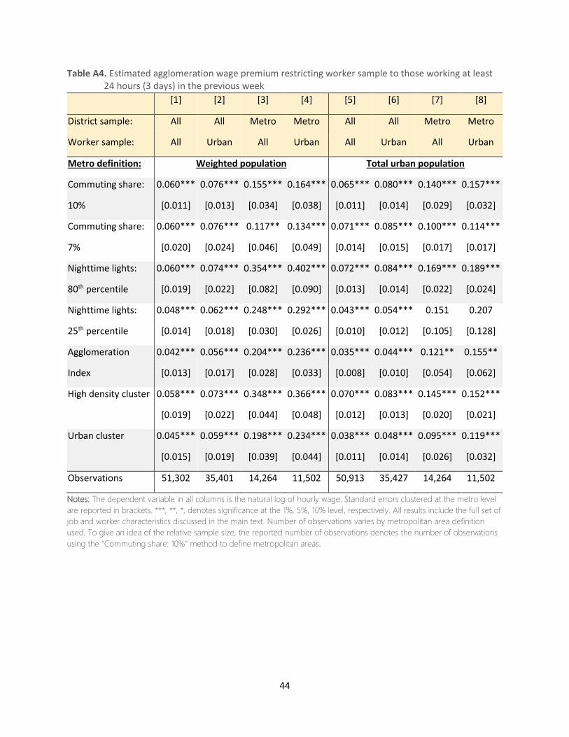
44

Table A4. Estimated agglomeration wage premium restricting worker sample to those working at least 24 hours (3 days) in the previous week

[1] [2] [3] [4] [5] [6] [7] [8]

District sample: All All Metro Metro All All Metro Metro

Worker sample: All Urban All Urban All Urban All Urban

Metro definition: Weighted population Total urban population

Commuting share: 0.060*** 0.076*** 0.155*** 0.164*** 0.065*** 0.080*** 0.140*** 0.157***

10% [0.011] [0.013] [0.034] [0.038] [0.011] [0.014] [0.029] [0.032]

Commuting share: 0.060*** 0.076*** 0.117** 0.134*** 0.071*** 0.085*** 0.100*** 0.114***

7% [0.020] [0.024] [0.046] [0.049] [0.014] [0.015] [0.017] [0.017]

Nighttime lights: 0.060*** 0.074*** 0.354*** 0.402*** 0.072*** 0.084*** 0.169*** 0.189***

80th percentile [0.019] [0.022] [0.082] [0.090] [0.013] [0.014] [0.022] [0.024]

Nighttime lights: 0.048*** 0.062*** 0.248*** 0.292*** 0.043*** 0.054*** 0.151 0.207

25th percentile [0.014] [0.018] [0.030] [0.026] [0.010] [0.012] [0.105] [0.128]

Agglomeration 0.042*** 0.056*** 0.204*** 0.236*** 0.035*** 0.044*** 0.121** 0.155**

Index [0.013] [0.017] [0.028] [0.033] [0.008] [0.010] [0.054] [0.062]

High density cluster 0.058*** 0.073*** 0.348*** 0.366*** 0.070*** 0.083*** 0.145*** 0.152***

[0.019] [0.022] [0.044] [0.048] [0.012] [0.013] [0.020] [0.021]

Urban cluster 0.045*** 0.059*** 0.198*** 0.234*** 0.038*** 0.048*** 0.095*** 0.119***

[0.015] [0.019] [0.039] [0.044] [0.011] [0.014] [0.026] [0.032]

Observations 51,302 35,401 14,264 11,502 50,913 35,427 14,264 11,502

Notes: The dependent variable in all columns is the natural log of hourly wage. Standard errors clustered at the metro level

are reported in brackets. ***, **, *, denotes significance at the 1%, 5%, 10% level, respectively. All results include the full set of

job and worker characteristics discussed in the main text. Number of observations varies by metropolitan area definition

used. To give an idea of the relative sample size, the reported number of observations denotes the number of observations

using the “Commuting share: 10%” method to define metropolitan areas.

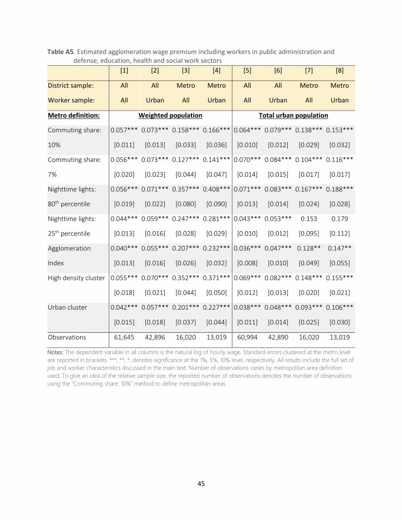
45

Table A5. Estimated agglomeration wage premium including workers in public administration and defense, education, health and social work sectors

[1] [2] [3] [4] [5] [6] [7] [8]

District sample: All All Metro Metro All All Metro Metro

Worker sample: All Urban All Urban All Urban All Urban

Metro definition: Weighted population Total urban population

Commuting share: 0.057*** 0.073*** 0.158*** 0.166*** 0.064*** 0.079*** 0.138*** 0.153***

10% [0.011] [0.013] [0.033] [0.036] [0.010] [0.012] [0.029] [0.032]

Commuting share: 0.056*** 0.073*** 0.127*** 0.141*** 0.070*** 0.084*** 0.104*** 0.116***

7% [0.020] [0.023] [0.044] [0.047] [0.014] [0.015] [0.017] [0.017]

Nighttime lights: 0.056*** 0.071*** 0.357*** 0.408*** 0.071*** 0.083*** 0.167*** 0.188***

80th percentile [0.019] [0.022] [0.080] [0.090] [0.013] [0.014] [0.024] [0.028]

Nighttime lights: 0.044*** 0.059*** 0.247*** 0.281*** 0.043*** 0.053*** 0.153 0.179

25th percentile [0.013] [0.016] [0.028] [0.029] [0.010] [0.012] [0.095] [0.112]

Agglomeration 0.040*** 0.055*** 0.207*** 0.232*** 0.036*** 0.047*** 0.128** 0.147**

Index [0.013] [0.016] [0.026] [0.032] [0.008] [0.010] [0.049] [0.055]

High density cluster 0.055*** 0.070*** 0.352*** 0.371*** 0.069*** 0.082*** 0.148*** 0.155***

[0.018] [0.021] [0.044] [0.050] [0.012] [0.013] [0.020] [0.021]

Urban cluster 0.042*** 0.057*** 0.201*** 0.227*** 0.038*** 0.048*** 0.093*** 0.106***

[0.015] [0.018] [0.037] [0.044] [0.011] [0.014] [0.025] [0.030]

Observations 61,645 42,896 16,020 13,019 60,994 42,890 16,020 13,019

Notes: The dependent variable in all columns is the natural log of hourly wage. Standard errors clustered at the metro level

are reported in brackets. ***, **, *, denotes significance at the 1%, 5%, 10% level, respectively. All results include the full set of

job and worker characteristics discussed in the main text. Number of observations varies by metropolitan area definition

used. To give an idea of the relative sample size, the reported number of observations denotes the number of observations

using the “Commuting share: 10%” method to define metropolitan areas.

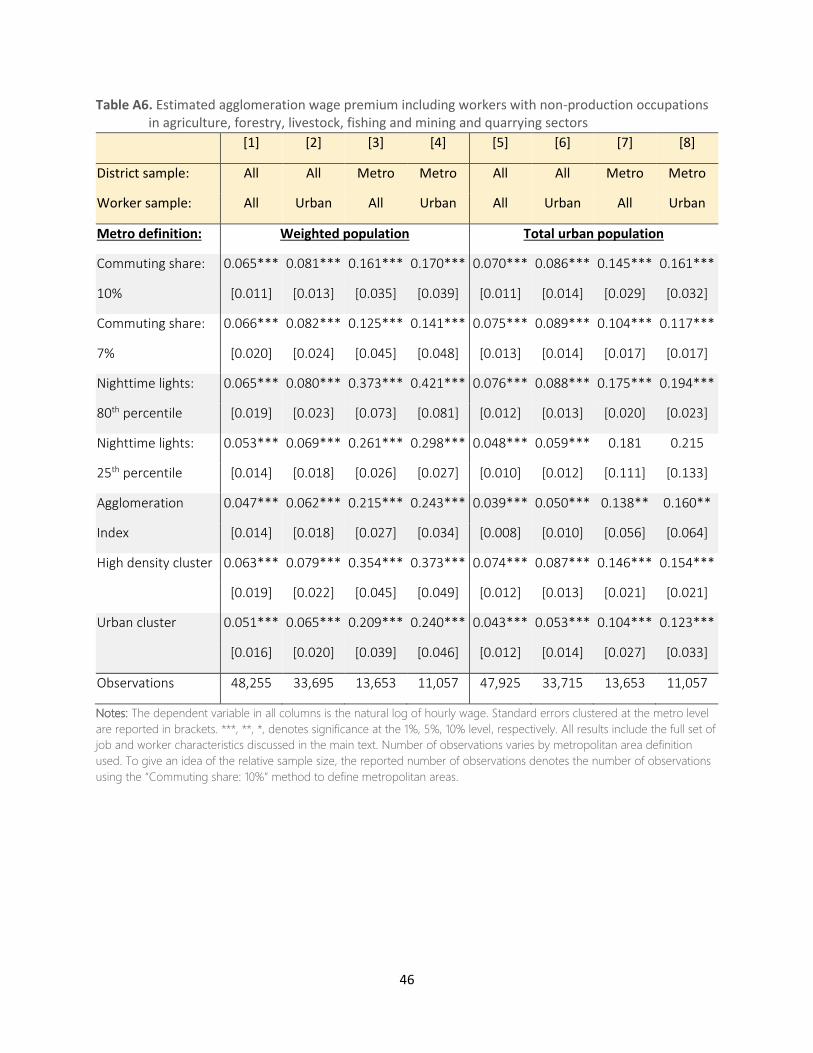
46

Table A6. Estimated agglomeration wage premium including workers with non-production occupations in agriculture, forestry, livestock, fishing and mining and quarrying sectors

[1] [2] [3] [4] [5] [6] [7] [8]

District sample: All All Metro Metro All All Metro Metro

Worker sample: All Urban All Urban All Urban All Urban

Metro definition: Weighted population Total urban population

Commuting share: 0.065*** 0.081*** 0.161*** 0.170*** 0.070*** 0.086*** 0.145*** 0.161***

10% [0.011] [0.013] [0.035] [0.039] [0.011] [0.014] [0.029] [0.032]

Commuting share: 0.066*** 0.082*** 0.125*** 0.141*** 0.075*** 0.089*** 0.104*** 0.117***

7% [0.020] [0.024] [0.045] [0.048] [0.013] [0.014] [0.017] [0.017]

Nighttime lights: 0.065*** 0.080*** 0.373*** 0.421*** 0.076*** 0.088*** 0.175*** 0.194***

80th percentile [0.019] [0.023] [0.073] [0.081] [0.012] [0.013] [0.020] [0.023]

Nighttime lights: 0.053*** 0.069*** 0.261*** 0.298*** 0.048*** 0.059*** 0.181 0.215

25th percentile [0.014] [0.018] [0.026] [0.027] [0.010] [0.012] [0.111] [0.133]

Agglomeration 0.047*** 0.062*** 0.215*** 0.243*** 0.039*** 0.050*** 0.138** 0.160**

Index [0.014] [0.018] [0.027] [0.034] [0.008] [0.010] [0.056] [0.064]

High density cluster 0.063*** 0.079*** 0.354*** 0.373*** 0.074*** 0.087*** 0.146*** 0.154***

[0.019] [0.022] [0.045] [0.049] [0.012] [0.013] [0.021] [0.021]

Urban cluster 0.051*** 0.065*** 0.209*** 0.240*** 0.043*** 0.053*** 0.104*** 0.123***

[0.016] [0.020] [0.039] [0.046] [0.012] [0.014] [0.027] [0.033]

Observations 48,255 33,695 13,653 11,057 47,925 33,715 13,653 11,057

Notes: The dependent variable in all columns is the natural log of hourly wage. Standard errors clustered at the metro level

are reported in brackets. ***, **, *, denotes significance at the 1%, 5%, 10% level, respectively. All results include the full set of

job and worker characteristics discussed in the main text. Number of observations varies by metropolitan area definition

used. To give an idea of the relative sample size, the reported number of observations denotes the number of observations

using the “Commuting share: 10%” method to define metropolitan areas.

47

Table A7. Estimated agglomeration wage premium restricting worker sample to employees (i.e., excluding own account workers)

[1] [2] [3] [4] [5] [6] [7] [8]

District sample: All All Metro Metro All All Metro Metro

Worker sample: All Urban All Urban All Urban All Urban

Metro definition: Weighted population Total urban population

Commuting share: 0.076*** 0.092*** 0.179*** 0.188*** 0.079*** 0.096*** 0.158*** 0.175***

10% [0.013] [0.016] [0.040] [0.044] [0.013] [0.017] [0.033] [0.037]

Commuting share: 0.077*** 0.092*** 0.144*** 0.158*** 0.085*** 0.100*** 0.117*** 0.130***

7% [0.024] [0.028] [0.051] [0.055] [0.015] [0.017] [0.019] [0.020]

Nighttime lights: 0.075*** 0.090*** 0.403*** 0.447*** 0.086*** 0.099*** 0.189*** 0.208***

80th percentile [0.023] [0.027] [0.075] [0.089] [0.014] [0.016] [0.026] [0.030]

Nighttime lights: 0.064*** 0.079*** 0.300*** 0.332*** 0.058*** 0.073*** 0.251* 0.291*

25th percentile [0.017] [0.021] [0.024] [0.023] [0.011] [0.014] [0.126] [0.145]

Agglomeration 0.057*** 0.071*** 0.242*** 0.268*** 0.049*** 0.062*** 0.178** 0.201**

Index [0.016] [0.020] [0.029] [0.035] [0.009] [0.012] [0.061] [0.071]

High density cluster 0.072*** 0.088*** 0.407*** 0.427*** 0.084*** 0.098*** 0.169*** 0.177***

[0.022] [0.026] [0.057] [0.062] [0.014] [0.015] [0.023] [0.024]

Urban cluster 0.060*** 0.074*** 0.242*** 0.272*** 0.053*** 0.065*** 0.129*** 0.152***

[0.019] [0.024] [0.046] [0.053] [0.014] [0.017] [0.034] [0.041]

Observations 33,027 23,923 10,603 8,679 32,835 23,930 10,603 8,679

Notes: The dependent variable in all columns is the natural log of hourly wage. Standard errors clustered at the metro level

are reported in brackets. ***, **, *, denotes significance at the 1%, 5%, 10% level, respectively. All results include the full set of

job and worker characteristics discussed in the main text. Number of observations varies by metropolitan area definition

used. To give an idea of the relative sample size, the reported number of observations denotes the number of observations

using the “Commuting share: 10%” method to define metropolitan areas.

48

Table A8. Estimated agglomeration wage premium measuring hourly wage using cash income only

[1] [2] [3] [4] [5] [6] [7] [8]

District sample: All All Metro Metro All All Metro Metro

Worker sample: All Urban All Urban All Urban All Urban

Metro definition: Weighted population Total urban population

Commuting share: 0.068*** 0.084*** 0.170*** 0.181*** 0.072*** 0.088*** 0.154*** 0.173***

10% [0.011] [0.014] [0.035] [0.039] [0.011] [0.014] [0.029] [0.032]

Commuting share: 0.068*** 0.084*** 0.130*** 0.147*** 0.077*** 0.091*** 0.108*** 0.121***

7% [0.021] [0.024] [0.046] [0.049] [0.014] [0.014] [0.017] [0.017]

Nighttime lights: 0.067*** 0.082*** 0.374*** 0.420*** 0.078*** 0.090*** 0.176*** 0.195***

80th percentile [0.020] [0.023] [0.077] [0.086] [0.012] [0.014] [0.020] [0.023]

Nighttime lights: 0.054*** 0.069*** 0.264*** 0.301*** 0.049*** 0.061*** 0.182 0.216

25th percentile [0.014] [0.018] [0.026] [0.027] [0.010] [0.012] [0.113] [0.135]

Agglomeration 0.048*** 0.062*** 0.218*** 0.245*** 0.040*** 0.051*** 0.139** 0.161**

Index [0.014] [0.018] [0.027] [0.034] [0.008] [0.010] [0.057] [0.065]

High density cluster 0.065*** 0.080*** 0.364*** 0.382*** 0.076*** 0.089*** 0.149*** 0.156***

[0.020] [0.023] [0.044] [0.048] [0.012] [0.013] [0.021] [0.021]

Urban cluster 0.051*** 0.065*** 0.211*** 0.242*** 0.043*** 0.053*** 0.104*** 0.123***

[0.016] [0.020] [0.040] [0.046] [0.012] [0.015] [0.027] [0.033]

Observations 47,498 33,237 13,607 11,015 47,185 33,259 13,607 11,015

Notes: The dependent variable in all columns is the natural log of hourly wage in cash. Standard errors clustered at the

metro level are reported in brackets. ***, **, *, denotes significance at the 1%, 5%, 10% level, respectively. All results include

the full set of job and worker characteristics discussed in the main text. Number of observations varies by metropolitan area

definition used. To give an idea of the relative sample size, the reported number of observations denotes the number of

observations using the “Commuting share: 10%” method to define metropolitan areas.

49

Table A9. Total Urban Population instead of De La Roca and Puga (2017)’s weighted population

[1] [2] [3] [4] [5] [6] [7] [8]

District sample: All All Metro Metro All All Metro Metro

Worker sample: All Urban All Urban All Urban All Urban

Metro definition: OLS 2SLS

District 0.079*** 0.100*** 0.193*** 0.228***

[0.010] [0.013] [0.035] [0.046]

Duranton: 10 % 0.070*** 0.086*** 0.145*** 0.161*** 0.152*** 0.176*** 0.201*** 0.222***

[0.011] [0.014] [0.029] [0.032] [0.028] [0.035] [0.038] [0.042]

Duranton: 7 % 0.075*** 0.089*** 0.103*** 0.116*** 0.122*** 0.135*** 0.151*** 0.162***

[0.013] [0.014] [0.017] [0.017] [0.017] [0.020] [0.026] [0.027]

NTL: 80th percentile 0.076*** 0.088*** 0.174*** 0.194*** 0.122*** 0.136*** 0.336** 1.737

[0.012] [0.013] [0.020] [0.023] [0.017] [0.021] [0.101] [12.277]

NTL: 25th percentile 0.048*** 0.059*** 0.18 0.214 0.146** 0.175** 0.825* 0.366***

[0.010] [0.012] [0.111] [0.133] [0.057] [0.075] [0.421] [0.099]

AI 0.039*** 0.050*** 0.138** 0.160** 0.149** 0.177** 0.35 0.092*

[0.008] [0.010] [0.056] [0.064] [0.066] [0.085] [0.230] [0.049]

Cluster algorithm 0.074*** 0.087*** 0.146*** 0.153*** 0.122*** 0.133*** 0.155*** 0.162***

(High density) [0.012] [0.013] [0.021] [0.021] [0.016] [0.018] [0.028] [0.030]

Cluster algorithm 0.043*** 0.053*** 0.104*** 0.123*** 0.145*** 0.172*** 0.237** 0.285**

(Urban cluster) [0.012] [0.014] [0.027] [0.033] [0.050] [0.063] [0.094] [0.113]

n 47,200 33,265 13,610 11,018 47,200 33,265 13,610 11,018

Notes: The dependent variable in all columns is the log of hourly wage. Standard errors clustered at the metro level are

reported in brackets. ***, **, *, denotes significance at the 1 percent, 5 percent and 10 percent levels respectively. All results

include the full set of job and worker characteristics discussed in Section 4.1.1. Number of observations varies by metro

definition used. To give an idea of the relative sample size across the different (restricted) samples, the reported number of

observations denotes the number of observations using the “Duranton: 10 %” approach to define metro areas. In columns

[5] – [8], the urban population measure (in natural log) is instrumented using the set of instruments set out in the text above

Table 5. Instruments are generally relevant, and pass the usual overidentification test(s). First stage results are available upon

request.

50

Table A10. Estimated agglomeration wage premium using different population thresholds to match administrative districts to the urban extents identified by the different “satellite-data based” algorithms.

[1] [2] [3] [4]

District sample: All All Metro Metro

Worker sample: All Urban All Urban

Metro definition: Population threshold Weighted population

NTL: 80th percentile 60% 0.062*** 0.078*** 0.476*** 0.526***

[0.020] [0.023] [0.093] [0.103]

NTL: 80th percentile 70% 0.066*** 0.082*** 0.424*** 0.445***

[0.021] [0.024] [0.082] [0.081]

NTL: 80th percentile 80% 0.066*** 0.082*** 0.474*** 0.484***

[0.020] [0.023] [0.048] [0.047]

NTL: 25th percentile 60% 0.053*** 0.069*** 0.237*** 0.275***

[0.013] [0.016] [0.043] [0.050]

NTL: 25th percentile 70% 0.059*** 0.075*** 0.229*** 0.266***

[0.014] [0.017] [0.045] [0.049]

NTL: 25th percentile 80% 0.061*** 0.076*** 0.339*** 0.383***

[0.018] [0.021] [0.048] [0.052]

Agglomeration Index 60% 0.049*** 0.063*** 0.213*** 0.239***

[0.013] [0.017] [0.030] [0.037]

Agglomeration Index 70% 0.049*** 0.064*** 0.233*** 0.256***

[0.013] [0.017] [0.037] [0.047]

Agglomeration Index 80% 0.050*** 0.063*** 0.252*** 0.277***

[0.012] [0.015] [0.053] [0.065]

High Density Cluster 60% 0.063*** 0.079*** 0.359*** 0.379***

[0.019] [0.022] [0.048] [0.052]

High Density Cluster 70% 0.062*** 0.078*** 0.347*** 0.366***

[0.019] [0.022] [0.062] [0.067]

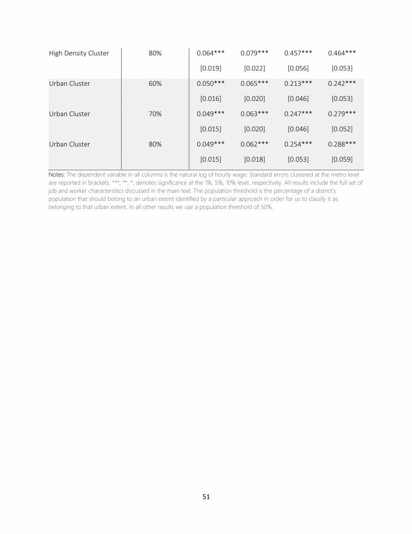
51

High Density Cluster 80% 0.064*** 0.079*** 0.457*** 0.464***

[0.019] [0.022] [0.056] [0.053]

Urban Cluster 60% 0.050*** 0.065*** 0.213*** 0.242***

[0.016] [0.020] [0.046] [0.053]

Urban Cluster 70% 0.049*** 0.063*** 0.247*** 0.279***

[0.015] [0.020] [0.046] [0.052]

Urban Cluster 80% 0.049*** 0.062*** 0.254*** 0.288***

[0.015] [0.018] [0.053] [0.059]

Notes: The dependent variable in all columns is the natural log of hourly wage. Standard errors clustered at the metro level

are reported in brackets. ***, **, *, denotes significance at the 1%, 5%, 10% level, respectively. All results include the full set of

job and worker characteristics discussed in the main text. The population threshold is the percentage of a district’s

population that should belong to an urban extent identified by a particular approach in order for us to classify it as

belonging to that urban extent. In all other results we use a population threshold of 50%.

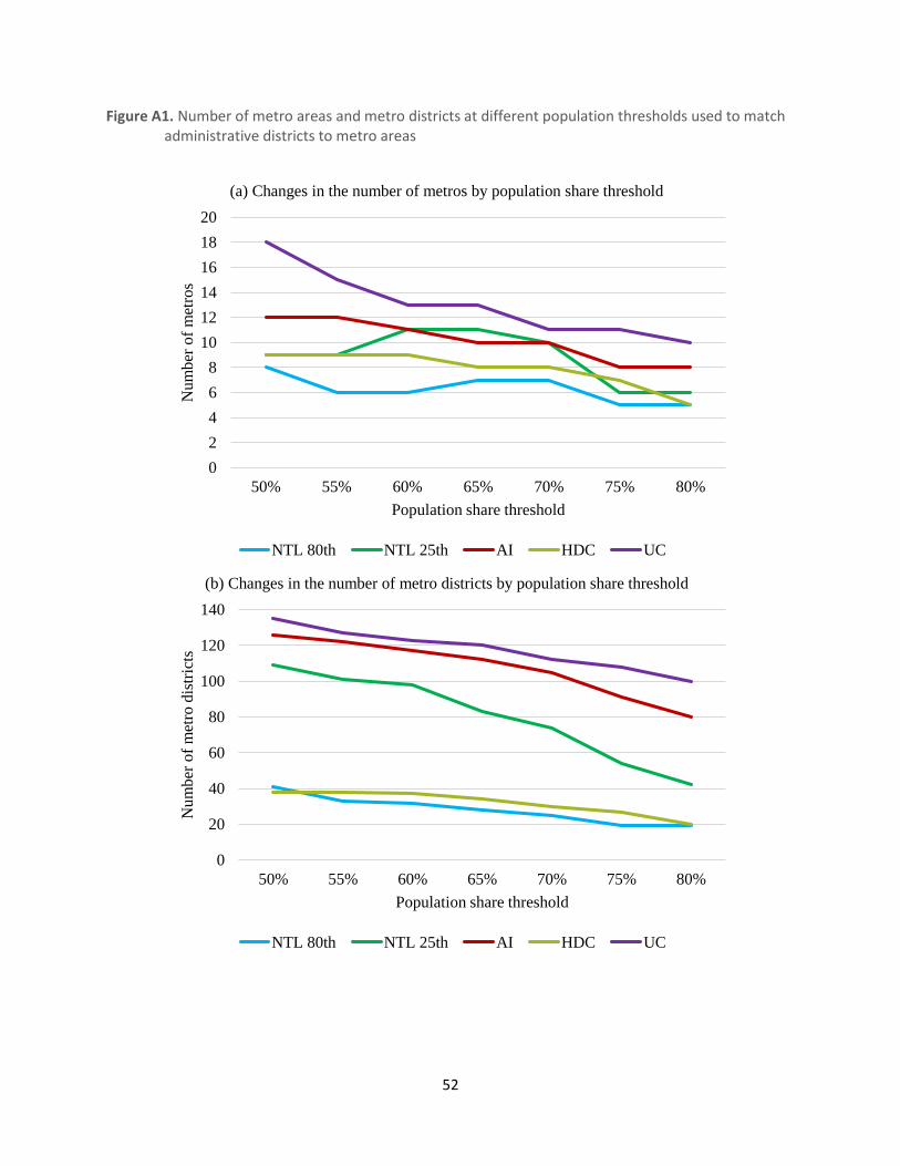
52

Figure A1. Number of metro areas and metro districts at different population thresholds used to match administrative districts to metro areas

(a) Changes in the number of metros by population share threshold

(b) Changes in the number of metro districts by population share threshold

0

2

4

6

8

10

12

14

16

18

20

50% 55% 60% 65% 70% 75% 80%

Nu

mb

er o

f m

etro

s

Population share threshold

NTL 80th NTL 25th AI HDC UC

0

20

40

60

80

100

120

140

50% 55% 60% 65% 70% 75% 80%

Nu

mber

of

met

ro d

istr

icts

Population share threshold

NTL 80th NTL 25th AI HDC UC

53

Figure A2. Evolution of metro areas from 10% to 7% cross-district commuting share

Figure A3. 2SLS estimates of the agglomeration wage premium across different thresholds (IVs: elevation, ruggedness, temperature, and rainfall)

(a) Commuting shares in combination with weighted population

(b) Nighttime lights in combination with weighted population

Notes: In panel (a), the use of a commuting threshold larger than 17% results in estimates of β that are larger than 2. We do

not show these in the figures as including them would blur the pattern observed when using thresholds smaller than 17%.

Furthermore, using thresholds above 17% results in an unrealistic definition of metropolitan areas (as discussed in Section

2.2). These figures are based on running 2SLS regressions, where our weighted population measure (in natural log) is

instrumented using the set of instruments set out in the text above Table 5. Instruments are generally relevant, and pass the

usual overidentification test(s). First stage results are available upon request.