Deformation Analysis of Large Diameter Monopiles of

applied sciences

Article

Deformation Analysis of Large Diameter Monopilesof Offshore Wind Turbines under Scour

Zhaoyao Wang 1, Ruigeng Hu 1, Hao Leng 1, Hongjun Liu 1,2,*, Yifan Bai 3 and Wenyan Lu 3

1 College of Environmental Science and Engineering, Ocean University of China, Qingdao 266100, China;[email protected] (Z.W.); [email protected] (R.H.); [email protected] (H.L.)

2 Shandong Provincial Key Laboratory of Marine Environment and Geological Engineering,Qingdao 266100, China

3 School of Civil Engineering, Shandong Jianzhu University, Jinan 250101, China;[email protected] (Y.B.); [email protected] (W.L.)

* Correspondence: [email protected]; Tel.: +86-532-66782571

Received: 27 July 2020; Accepted: 7 September 2020; Published: 28 October 2020

Abstract: The displacement of monopile supporting offshore wind turbines needs to be strictlycontrolled, and the influence of local scour can not be ignored. Using p–y curves to simulate thepile–soil interaction and the finite difference method to calculate iteratively, a numerical frame foranalysis of lateral loaded pile was discussed and then verified. On the basis of the field data fromDafeng Offshore Wind Farm in Jiangsu Province, the local scour characteristics of large diametermonopile were concluded, and a new method of considering scour effect applicable to large diametermonopile was put forward. The results show that, for scour of large diameter monopiles, there was noobvious scour pit, but local erosion and deposition. Under the test conditions, the displacement errorsbetween the proposed and traditional method were 46.4%. By the proposed method, the p–y curvesof monopile considering the scour effect were obtained through ABAQUS, and the deformation oflarge diameter monopile under scour was analyzed by the proposed frame. The results show that,with the increase of scour depth, the horizontal displacement of the pile head increases nonlinearly,the depth of rotation point moves downward, and both of the changes are related to the load level.Under the test conditions, the horizontal displacement of the pile head after scour could reach 1.4~3.6times of that before scour. Finally, for different pile parameters, the pile head displacement wascompared, and further, the susceptibility to scour was quantified by a proposed concept of scoursensitivity. The analysis indicates that increasing pile length is a more reasonable way than pilediameter and wall thickness to limit the scour effect on the displacement of large diameter pile.

Keywords: pile foundations; offshore wind turbines; scour; p–y curve; finite difference method;horizontal displacement

1. Introduction

In offshore wind power projects, the foundation design accounts for about 25% of the totalcost [1], and the foundation serviceability is of importance for the normal operation of wind turbines.Large diameter monopile (Figure 1) is widely used in practical engineering, with its advantages ofsuperior economy and reliability [2].

Under the environmental loading from waves and currents, the displacement of monopile can notexceed 0.5 of rotation at the mudline, or another similar value suggested by the turbine manufacturers,so it is necessary to study the deformation characteristics of large diameter monopile under horizontalloads. Owing to the harsh environmental conditions and high cost, the field test of large diametermonopile is difficult to carry out, hence the numerical analysis is more commonly used. Bouzid et al. [3]

Appl. Sci. 2020, 10, 7579; doi:10.3390/app10217579 www.mdpi.com/journal/applsci

http://www.mdpi.com/journal/applsci

http://www.mdpi.com

http://www.mdpi.com/2076-3417/10/21/7579?type=check_update&version=1

http://dx.doi.org/10.3390/app10217579

http://www.mdpi.com/journal/applsci

Appl. Sci. 2020, 10, 7579 2 of 18

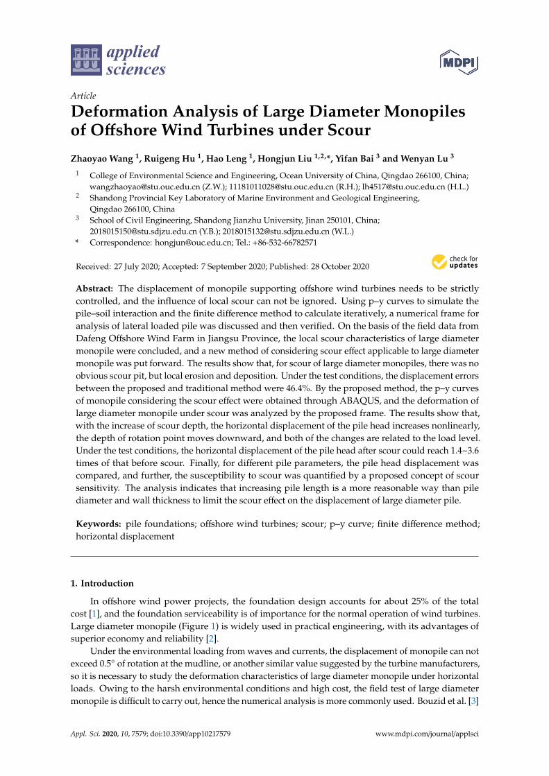
pointed out that the finite element method is effective for the assessment of lateral loaded monopileand the conventional p–y curve method derived from field tests of a small diameter is not suitablefor large diameter monopile. Achmus et al. [4] evaluated the effect of pile diameter on p–y curves.Zhang et al. [5] proposed a p–y curve construction method for large diameter monopile, and takesthe roughness of the pile–soil interface into account. Lee et al. [6] studied the cyclic effects on the p–ycurve by centrifugal model test. Under the coupled waves and currents, local scour occurs around thepile foundation, which affects the static and dynamic response of monopile [7–9]. Therefore, the scoureffect must be considered in the deformation analysis. He et al. [10] and Carswell et al. [11] reducedthe buried depth of pile foundation by removing a certain depth of soil layer (Figure 2). Dai et al. [12]considered the scour pit features and introduced a wedge-shaped failure mechanism to express theinfluence of local scour.Appl. Sci. 2020, 10, x FOR PEER REVIEW 2 of 19

0 1 2 3 4 5 6 7 8 9 100

10

20

30

40

50

60

70

80

90

100

D=3

pile

leng

th L

/ m

pile diameter D / m

L/D=10

large diameter monopile

Figure 1. Generally accepted concept of large diameter monopile.

Under the environmental loading from waves and currents, the displacement of monopile can not exceed 0.5° of rotation at the mudline, or another similar value suggested by the turbine manufacturers, so it is necessary to study the deformation characteristics of large diameter monopile under horizontal loads. Owing to the harsh environmental conditions and high cost, the field test of large diameter monopile is difficult to carry out, hence the numerical analysis is more commonly used. Bouzid et al. [3] pointed out that the finite element method is effective for the assessment of lateral loaded monopile and the conventional p–y curve method derived from field tests of a small diameter is not suitable for large diameter monopile. Achmus et al. [4] evaluated the effect of pile diameter on p–y curves. Zhang et al. [5] proposed a p–y curve construction method for large diameter monopile, and takes the roughness of the pile–soil interface into account. Lee et al. [6] studied the cyclic effects on the p–y curve by centrifugal model test. Under the coupled waves and currents, local scour occurs around the pile foundation, which affects the static and dynamic response of monopile [7–9]. Therefore, the scour effect must be considered in the deformation analysis. He et al. [10] and Carswell et al. [11] reduced the buried depth of pile foundation by removing a certain depth of soil layer (Figure 2). Dai et al. [12] considered the scour pit features and introduced a wedge-shaped failure mechanism to express the influence of local scour.

Figure 2. Embedment reduction diagram.

It can be seen that, for the analysis of large diameter monopile of offshore wind turbines, horizontal deformation characteristic is of significance, and appropriate methods should be selected. The p–y curve method is widely used and it is crucial to obtain the p–y curve suitable for large diameter monopile. Secondly, as for local scour, both the scour characteristic and scour effect consideration method lack the support of field data, as they only took the maximum scour depth into consideration instead of the scour pattern, and whether they are applicable to large diameter monopile remains uncertain. To quantitatively summarize the scour characteristics and the effect of large diameter monopile is helpful for offshore wind power construction and subsequent load and


Appl. Sci. 2020, 10, x FOR PEER REVIEW 2 of 19

0 1 2 3 4 5 6 7 8 9 100

10

20

30

40

50

60

70

80

90

100

D=3

pile

leng

th L

/ m

pile diameter D / m

L/D=10

large diameter monopile


Under the environmental loading from waves and currents, the displacement of monopile can not exceed 0.5° of rotation at the mudline, or another similar value suggested by the turbine manufacturers, so it is necessary to study the deformation characteristics of large diameter monopile under horizontal loads. Owing to the harsh environmental conditions and high cost, the field test of large diameter monopile is difficult to carry out, hence the numerical analysis is more commonly used. Bouzid et al. [3] pointed out that the finite element method is effective for the assessment of lateral loaded monopile and the conventional p–y curve method derived from field tests of a small diameter is not suitable for large diameter monopile. Achmus et al. [4] evaluated the effect of pile diameter on p–y curves. Zhang et al. [5] proposed a p–y curve construction method for large diameter monopile, and takes the roughness of the pile–soil interface into account. Lee et al. [6] studied the cyclic effects on the p–y curve by centrifugal model test. Under the coupled waves and currents, local scour occurs around the pile foundation, which affects the static and dynamic response of monopile [7–9]. Therefore, the scour effect must be considered in the deformation analysis. He et al. [10] and Carswell et al. [11] reduced the buried depth of pile foundation by removing a certain depth of soil layer (Figure 2). Dai et al. [12] considered the scour pit features and introduced a wedge-shaped failure mechanism to express the influence of local scour.


It can be seen that, for the analysis of large diameter monopile of offshore wind turbines, horizontal deformation characteristic is of significance, and appropriate methods should be selected. The p–y curve method is widely used and it is crucial to obtain the p–y curve suitable for large diameter monopile. Secondly, as for local scour, both the scour characteristic and scour effect consideration method lack the support of field data, as they only took the maximum scour depth into consideration instead of the scour pattern, and whether they are applicable to large diameter monopile remains uncertain. To quantitatively summarize the scour characteristics and the effect of large diameter monopile is helpful for offshore wind power construction and subsequent load and


It can be seen that, for the analysis of large diameter monopile of offshore wind turbines, horizontaldeformation characteristic is of significance, and appropriate methods should be selected. The p–ycurve method is widely used and it is crucial to obtain the p–y curve suitable for large diametermonopile. Secondly, as for local scour, both the scour characteristic and scour effect considerationmethod lack the support of field data, as they only took the maximum scour depth into considerationinstead of the scour pattern, and whether they are applicable to large diameter monopile remainsuncertain. To quantitatively summarize the scour characteristics and the effect of large diametermonopile is helpful for offshore wind power construction and subsequent load and displacementanalysis. In addition, few studies have focused on the displacement sensitivity of monopile under scour.

Therefore, this paper introduces the p–y curve method and the iterative procedure of finitedifference method, and verifies the accuracy of the horizontal displacement analysis frame by modeltest and field test. Then, on the basis of the scour monitoring data from Dafeng offshore wind farm

Appl. Sci. 2020, 10, 7579 3 of 18

in Jiangsu Province, we conclude the scour characteristics of large diameter monopile and propose amethod of considering the scour effect applicable to large diameter monopile. Finally, by the proposedmethod, we extract p–y curves of monopile considering the scour effect through ABAQUS, and analyzethe deformation characteristics of large diameter monopile under scour. The sensitivity of pile headdisplacement under scour is studied by analyzing the relationship among scour depth, pile headdisplacement, and pile parameters, and the concept of scouring sensitivity is proposed, which mayprovide ideas for practical engineering.

2. Deformation Analysis Method

2.1. p–y Curve

In the analysis of lateral loaded pile foundations, the soil is modeled as a system of uncoupledsprings distributed along the depth, and the pile response can be obtained from the differentialequation:

EIdy4

dx4+ p(x) = 0 (1)

where EI: pile bending stiffness, y: pile displacement, p: soil resistance, and X: length along the pile.The key to solving the differential equation is the soil resistance function p(x), which includes

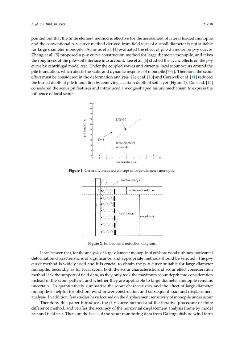
linear and nonlinear assumptions. The linear method assumes that the soil resistance p is proportionalto the pile displacement y at any depth, which means the stiffness of soil spring could be representedby a constant. The other solution assumes that the soil resistance function p(x) is non-linear, and thestiffness of soil spring could be described by p–y curves. Through field test or lab element test [13],the p–y curve at any depth under the mudline (Figure 3) could be constructed.


displacement analysis. In addition, few studies have focused on the displacement sensitivity of monopile under scour.

Therefore, this paper introduces the p–y curve method and the iterative procedure of finite difference method, and verifies the accuracy of the horizontal displacement analysis frame by model test and field test. Then, on the basis of the scour monitoring data from Dafeng offshore wind farm in Jiangsu Province, we conclude the scour characteristics of large diameter monopile and propose a method of considering the scour effect applicable to large diameter monopile. Finally, by the proposed method, we extract p–y curves of monopile considering the scour effect through ABAQUS, and analyze the deformation characteristics of large diameter monopile under scour. The sensitivity of pile head displacement under scour is studied by analyzing the relationship among scour depth, pile head displacement, and pile parameters, and the concept of scouring sensitivity is proposed, which may provide ideas for practical engineering.

2. Deformation Analysis Method

2.1. p–y Curve

In the analysis of lateral loaded pile foundations, the soil is modeled as a system of uncoupled springs distributed along the depth, and the pile response can be obtained from the differential equation:

4

4 ( ) 0dyEI p xdx

+ = (1)

where EI: pile bending stiffness, y: pile displacement, p: soil resistance, and X: length along the pile. The key to solving the differential equation is the soil resistance function p(x), which includes

linear and nonlinear assumptions. The linear method assumes that the soil resistance p is proportional to the pile displacement y at any depth, which means the stiffness of soil spring could be represented by a constant. The other solution assumes that the soil resistance function p(x) is non-linear, and the stiffness of soil spring could be described by p–y curves. Through field test or lab element test [13], the p–y curve at any depth under the mudline (Figure 3) could be constructed.

Figure 3. P–y curve at different depths and calculation diagram.

h

h

h

h ym-2

ym-1

ym

ym+1

ym+2

-2-10

123

456

n - 2n - 1

nn + 1n + 2 M0

Q0

y

x

y

y

p

py

p

Figure 3. P–y curve at different depths and calculation diagram.

Matlock [14] and Reese et al. [15] proposed p–y curves for soft clay and stiff clay, respectively,and Reese et al. [16] gave the expression of p–y curves in sand. American Petroleum Institute’srecommendations [17] are widely used in practical engineering. Wang et al. [18] proposed a methodapplicable to both soft and stiff clay. Table 1 lists several p–y curve models, and Wang et al. [19] madea review on the p–y curve for monotonic and cyclic and discussed problems in existing studies.

Appl. Sci. 2020, 10, 7579 4 of 18

Table 1. P–y curve empirical formula.

Soil Type Expression Notes

Soft clay(Matlock [14])

ppu

= 0.5( yy50

)1/3

, y ≤ 8

y50ppu

= 1, y > 8y50

pu: ultimate soil resistance; y50: displacement at half ofthe ultimate resistance

Clay(Wang et al. [18])

ppu

= (y/y50

a+by/y50), y ≤ β

y50ppu

= 1, y > βy50

A, b, β: parameter obtained from triaxial test

Sand (API [17]) p = Aputanh( KApu

y) A: empirical factor; K: subgrade modulus, K = kx (k isinitial subgrade modulus; x is the distance to mudline)

2.2. Iterative Solution of Finite Difference Equations

Once the p–y curve is obtained, it is difficult to solve the differential equations by the analyticalmethod. This paper solves the equations by finite difference iterative calculation [20]. The pile isdivided into n segments (Figure 3), and the derivative deflection equation could be replaced by thedifference equation:

ym−2 − 4ym−1 + (6 +Esh4

EI)ym − 4ym+1 + ym+2 = 0 (2)

After the process above, n + 1 difference equations would be obtained.The shear force and moment of pile tip is 0, so the boundary conditions at pile tip is as follows:

y−2 − 2y−1 + 2y1 − y2 = 0 (3)

y1 − 2y0 + y−1 = 0 (4)

The shear force and moment of pile head are given as Q0 and M0, so the boundary conditions atpile head are as follows:

yn−2 − 2yn−1 + 2yn+1 − yn+2 =2Q0h3

EI(5)

yn−1 − 2yn + yn+1 =M0h2

EI(6)

With n + 1 equations along the pile length, 2 equations at the pile tip, 2 equations at the pile head,a total of n + 5 equations are obtained and then solved according to the matrix. Before solving theequations, a value of soil modulus Esm should be pre-assumed and input to the iterative program, so thatthe pile displacement y could be output by solving the matrix, and thus the soil resistance p would begenerated according to the corresponding p–y curves. Thus, the calculated soil modulus Esc is obtainedfrom the known p and y, and compared with Esm. When the tolerance is small enough, the iterationstops and the calculation ends. Figure 4 shows the iteration flows and calculation algorithm.

2.3. Verification with Model Test

A model test was designed and then carried out to verify the accuracy of the method mentionedabove. In the experiment, the deformation response of monopile in silt was obtained, and then it wascompared with the result calculated by the p–y curve method.

2.3.1. Experiment Materials

The test chamber is a rectangle made of glass fiber reinforced plastics, and its size is annotatedin Figure 5. The external walls are supported by three layers of steel angle to prevent deformationcaused by excessive pressure in the chamber, and cardboard is padded between the steel angle and thetest chamber.

Appl. Sci. 2020, 10, 7579 5 of 18


Assume initial Esm

Start

Solve the matrix

Obtain y

Look up corresponding p-y curve

Calculate p/y

Obtain p

Obtain Esc

Esc-Esm≤tolerance?

Output y

End

Yes

No

Figure 4. Iteration flow of the finite difference method.


A model test was designed and then carried out to verify the accuracy of the method mentioned above. In the experiment, the deformation response of monopile in silt was obtained, and then it was compared with the result calculated by the p–y curve method.


The test chamber is a rectangle made of glass fiber reinforced plastics, and its size is annotated in Figure 5. The external walls are supported by three layers of steel angle to prevent deformation caused by excessive pressure in the chamber, and cardboard is padded between the steel angle and the test chamber.

(a)

(b)



Assume initial Esm

Start

Solve the matrix

Obtain y

Look up corresponding p-y curve

Calculate p/y

Obtain p

Obtain Esc

Esc-Esm≤tolerance?

Output y

End

Yes

No



A model test was designed and then carried out to verify the accuracy of the method mentioned above. In the experiment, the deformation response of monopile in silt was obtained, and then it was compared with the result calculated by the p–y curve method.


The test chamber is a rectangle made of glass fiber reinforced plastics, and its size is annotated in Figure 5. The external walls are supported by three layers of steel angle to prevent deformation caused by excessive pressure in the chamber, and cardboard is padded between the steel angle and the test chamber.

(a)

(b)


(c)

Figure 5. Model test: (a) photo of model pile and protection of strain gauges; (b) pore pressure monitoring system; (c) sketch of model test.

The model pile is made of stainless steel pipe with an outer diameter of 32 mm, an inner diameter of 30.6 mm, and a length of 1.5 m. The bending stiffness of the model pile is 1510 N·m2. Thirteen pairs of strain gauges of 120 Ω resistance were symmetrically set along both sides of the pile shaft and waterproofing was guaranteed. Eight pore pressure sensors were used to observe the dissipation of pore pressure in order to determine the degree of consolidation. The arrangement of strain gauges and pore pressure meters is shown in Figure 5.

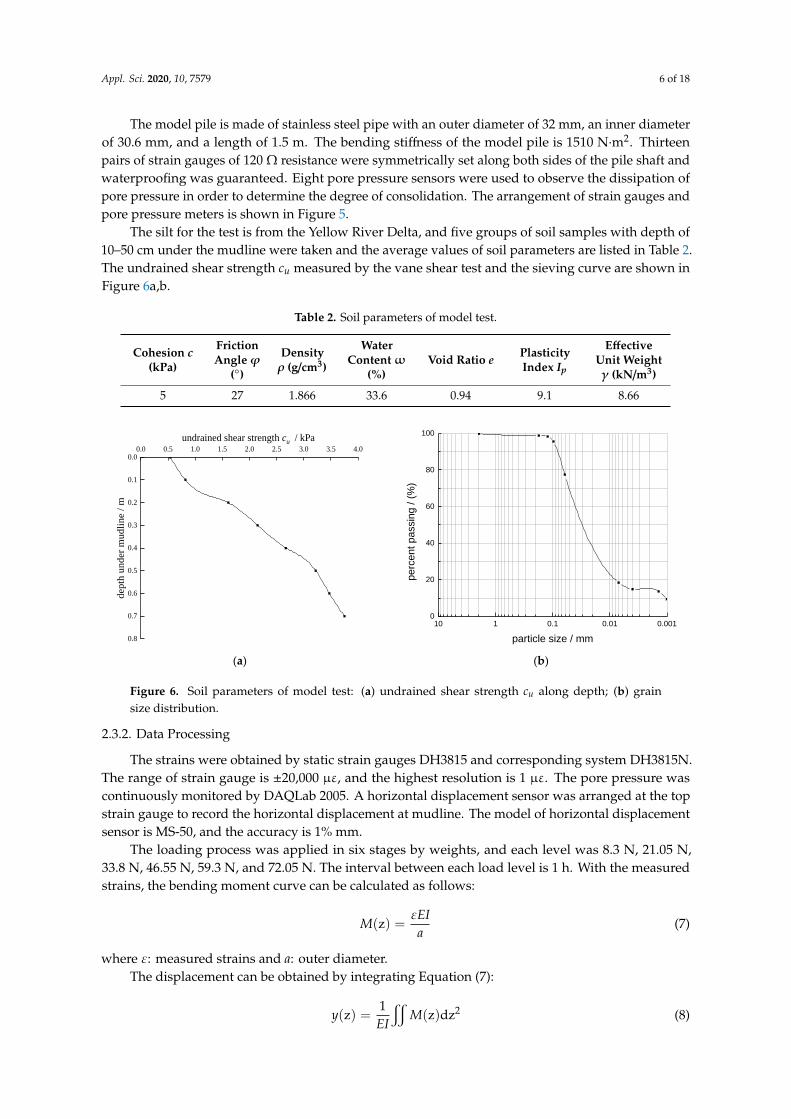
The silt for the test is from the Yellow River Delta, and five groups of soil samples with depth of 10–50 cm under the mudline were taken and the average values of soil parameters are listed in Table 2. The undrained shear strength cu measured by the vane shear test and the sieving curve are shown in Figure 6a,b.

Table 2. Soil parameters of model test.

Cohesionc (kPa)

Friction Angle φ

(°)

Density ρ (g/cm3)

Water Content ω (%)

Void Ratio e

Plasticity Index Ip

Effective Unit Weight γ (kN/m3)

5 27 1.866 33.6 0.94 9.1 8.66

(a) (b)

Figure 6. Soil parameters of model test: (a) undrained shear strength cu along depth; (b) grain size distribution.

Figure 5. Model test: (a) photo of model pile and protection of strain gauges; (b) pore pressuremonitoring system; (c) sketch of model test.

Appl. Sci. 2020, 10, 7579 6 of 18

The model pile is made of stainless steel pipe with an outer diameter of 32 mm, an inner diameterof 30.6 mm, and a length of 1.5 m. The bending stiffness of the model pile is 1510 N·m2. Thirteenpairs of strain gauges of 120 Ω resistance were symmetrically set along both sides of the pile shaft andwaterproofing was guaranteed. Eight pore pressure sensors were used to observe the dissipation ofpore pressure in order to determine the degree of consolidation. The arrangement of strain gauges andpore pressure meters is shown in Figure 5.

The silt for the test is from the Yellow River Delta, and five groups of soil samples with depth of10–50 cm under the mudline were taken and the average values of soil parameters are listed in Table 2.The undrained shear strength cu measured by the vane shear test and the sieving curve are shown inFigure 6a,b.


Cohesion c(kPa)

FrictionAngleϕ

()

Densityρ (g/cm3)

WaterContent ω

(%)Void Ratio e Plasticity

Index Ip

EffectiveUnit Weightγ (kN/m3)

5 27 1.866 33.6 0.94 9.1 8.66


(c)

Figure 5. Model test: (a) photo of model pile and protection of strain gauges; (b) pore pressure

monitoring system; (c) sketch of model test.

The model pile is made of stainless steel pipe with an outer diameter of 32 mm, an inner

diameter of 30.6 mm, and a length of 1.5 m. The bending stiffness of the model pile is 1510 N·m2.

Thirteen pairs of strain gauges of 120 Ω resistance were symmetrically set along both sides of the

pile shaft and waterproofing was guaranteed. Eight pore pressure sensors were used to observe the

dissipation of pore pressure in order to determine the degree of consolidation. The arrangement of

strain gauges and pore pressure meters is shown in Figure 5.

The silt for the test is from the Yellow River Delta, and five groups of soil samples with depth of

10–50 cm under the mudline were taken and the average values of soil parameters are listed in Table

2. The undrained shear strength cu measured by the vane shear test and the sieving curve are shown

in Figure 6a,b.


Cohesion

c (kPa)

Friction

Angle φ

(°)

Density ρ

(g/cm3)

Water

Content

ω (%)

Void

Ratio e

Plasticity

Index Ip

Effective

Unit Weight

γ (kN/m3)

5 27 1.866 33.6 0.94 9.1 8.66

0.0 0.5 1.0 1.5 2.0 2.5 3.0 3.5 4.0

0.8

0.7

0.6

0.5

0.4

0.3

0.2

0.1

0.0

undrained shear strength cu / kPa

depth

under

mudli

ne /

m

10 1 0.1 0.01 0.0010

20

40

60

80

100

perc

ent passin

g / (

%)

particle size / mm

(a) (b)

Figure 6. Soil parameters of model test: (a) undrained shear strength cu along depth; (b) grain size

distribution. Figure 6. Soil parameters of model test: (a) undrained shear strength cu along depth; (b) grainsize distribution.

2.3.2. Data Processing

The strains were obtained by static strain gauges DH3815 and corresponding system DH3815N.The range of strain gauge is ±20,000 µε, and the highest resolution is 1 µε. The pore pressure wascontinuously monitored by DAQLab 2005. A horizontal displacement sensor was arranged at the topstrain gauge to record the horizontal displacement at mudline. The model of horizontal displacementsensor is MS-50, and the accuracy is 1% mm.

The loading process was applied in six stages by weights, and each level was 8.3 N, 21.05 N,33.8 N, 46.55 N, 59.3 N, and 72.05 N. The interval between each load level is 1 h. With the measuredstrains, the bending moment curve can be calculated as follows:

M(z) =εEI

a(7)

where ε: measured strains and a: outer diameter.The displacement can be obtained by integrating Equation (7):

y(z) =1EI

xM(z)dz2 (8)

Appl. Sci. 2020, 10, 7579 7 of 18

2.3.3. Result Analysis

The p–y curve for silt was given by Wang et al. [21]:

p = Aputanh(Kpu

y) (9)

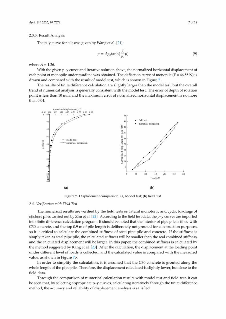
where A = 1.26.With the given p–y curve and iterative solution above, the normalized horizontal displacement of

each point of monopile under mudline was obtained. The deflection curve of monopile (F = 46.55 N) isdrawn and compared with the result of model test, which is shown in Figure 7.

The results of finite difference calculation are slightly larger than the model test, but the overalltrend of numerical analysis is generally consistent with the model test. The error of depth of rotationpoint is less than 10 mm, and the maximum error of normalized horizontal displacement is no morethan 0.04.


2.3.2. Data Processing

The strains were obtained by static strain gauges DH3815 and corresponding system DH3815N. The range of strain gauge is ±20,000 με, and the highest resolution is 1 με. The pore pressure was continuously monitored by DAQLab 2005. A horizontal displacement sensor was arranged at the top strain gauge to record the horizontal displacement at mudline. The model of horizontal displacement sensor is MS-50, and the accuracy is 1% mm.

The loading process was applied in six stages by weights, and each level was 8.3 N, 21.05 N, 33.8 N, 46.55 N, 59.3 N, and 72.05 N. The interval between each load level is 1 h. With the measured strains, the bending moment curve can be calculated as follows:

(z) EIMa

ε=

(7)

where ε: measured strains and a: outer diameter. The displacement can be obtained by integrating Equation (7):

21(z) (z) dzy MEI

= (8)

2.3.3. Result Analysis

The p–y curve for silt was given by Wang et al. [21]:

tanh( )uu

Kp Ap yp

=

(9)

where A = 1.26. With the given p–y curve and iterative solution above, the normalized horizontal displacement

of each point of monopile under mudline was obtained. The deflection curve of monopile (F = 46.55 N) is drawn and compared with the result of model test, which is shown in Figure 7.

The results of finite difference calculation are slightly larger than the model test, but the overall trend of numerical analysis is generally consistent with the model test. The error of depth of rotation point is less than 10 mm, and the maximum error of normalized horizontal displacement is no more than 0.04.

(a) (b)

Figure 7. Displacement comparison. (a) Model test; (b) field test.

0.9

0.8

0.7

0.6

0.5

0.4

0.3

0.2

0.1

0.0-0.05 0.00 0.05 0.10 0.15 0.20 0.25 0.30 0.35

normalized displacement y/D

dept

h /m

model test numerical calculation

0 50 100 150 200 250 300

5

10

15

20

25

30

35

40

45

50

norm

aliz

ed d

ispla

cem

ent y

/D /1

0-3

Load /kN

field test numerical calculation

Figure 7. Displacement comparison. (a) Model test; (b) field test.

2.4. Verification with Field Test

The numerical results are verified by the field tests on lateral monotonic and cyclic loadings ofoffshore piles carried out by Zhu et al. [22]. According to the field test data, the p–y curves are importedinto finite difference calculation program. It should be noted that the interior of pipe pile is filled withC30 concrete, and the top 0.9 m of pile length is deliberately not grouted for construction purposes,so it is critical to calculate the combined stiffness of steel pipe pile and concrete. If the stiffness issimply taken as steel pipe pile, the calculated stiffness will be smaller than the real combined stiffness,and the calculated displacement will be larger. In this paper, the combined stiffness is calculated bythe method suggested by Kang et al. [23]. After the calculation, the displacement at the loading pointunder different level of loads is collected, and the calculated value is compared with the measuredvalue, as shown in Figure 7b.

In order to simplify the calculation, it is assumed that the C30 concrete is grouted along thewhole length of the pipe pile. Therefore, the displacement calculated is slightly lower, but close to thefield data.

Through the comparison of numerical calculation results with model test and field test, it canbe seen that, by selecting appropriate p–y curves, calculating iteratively through the finite differencemethod, the accuracy and reliability of displacement analysis is satisfied.

Appl. Sci. 2020, 10, 7579 8 of 18

3. Consideration of Local Scour

To study the influence of local scour on monopile, the scour characteristic must be clarified,which is the basis and reference for the scour effect. On the basis of the Dafeng Offshore Wind Farm inJiangsu Province, scour around large diameter monopile was surveyed and data including mudlinealtitude, erosion or deposition volume, maximum scour depth, and topographic fluctuation changeswere collected. The water depth is 8~14 m, the wave height is 1~2 m, and designed pile outer diameteris 5.5 m. Besides pile 49#~52#, which were not investigated owing to weather conditions, a total of 68sets of data were obtained.

3.1. Investigation Equipment

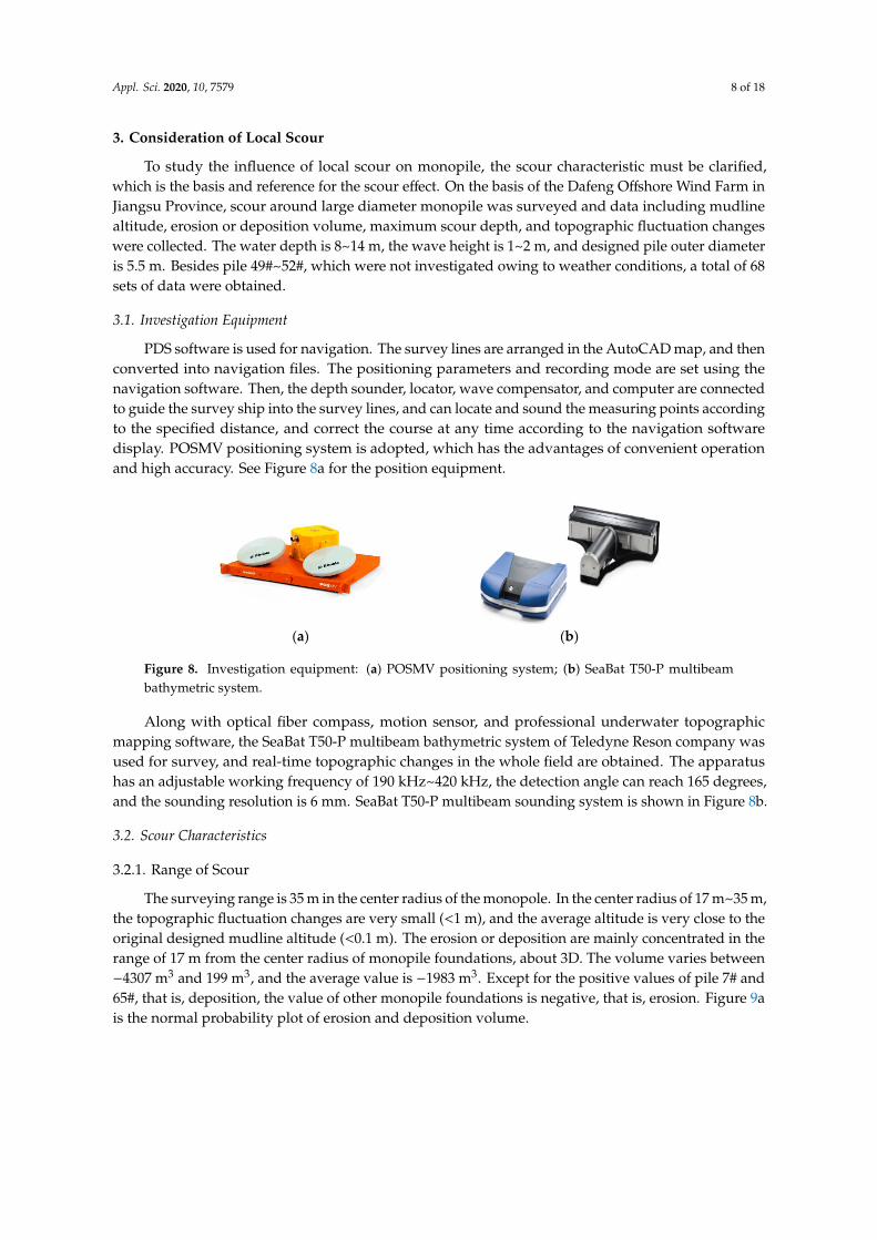
PDS software is used for navigation. The survey lines are arranged in the AutoCAD map, and thenconverted into navigation files. The positioning parameters and recording mode are set using thenavigation software. Then, the depth sounder, locator, wave compensator, and computer are connectedto guide the survey ship into the survey lines, and can locate and sound the measuring points accordingto the specified distance, and correct the course at any time according to the navigation softwaredisplay. POSMV positioning system is adopted, which has the advantages of convenient operationand high accuracy. See Figure 8a for the position equipment.


2.4. Verification with Field Test

The numerical results are verified by the field tests on lateral monotonic and cyclic loadings of offshore piles carried out by Zhu et al. [22]. According to the field test data, the p–y curves are imported into finite difference calculation program. It should be noted that the interior of pipe pile is filled with C30 concrete, and the top 0.9 m of pile length is deliberately not grouted for construction purposes, so it is critical to calculate the combined stiffness of steel pipe pile and concrete. If the stiffness is simply taken as steel pipe pile, the calculated stiffness will be smaller than the real combined stiffness, and the calculated displacement will be larger. In this paper, the combined stiffness is calculated by the method suggested by Kang et al. [23]. After the calculation, the displacement at the loading point under different level of loads is collected, and the calculated value is compared with the measured value, as shown in Figure 7b.

In order to simplify the calculation, it is assumed that the C30 concrete is grouted along the whole length of the pipe pile. Therefore, the displacement calculated is slightly lower, but close to the field data.

Through the comparison of numerical calculation results with model test and field test, it can be seen that, by selecting appropriate p–y curves, calculating iteratively through the finite difference method, the accuracy and reliability of displacement analysis is satisfied.

3. Consideration of Local Scour

To study the influence of local scour on monopile, the scour characteristic must be clarified, which is the basis and reference for the scour effect. On the basis of the Dafeng Offshore Wind Farm in Jiangsu Province, scour around large diameter monopile was surveyed and data including mudline altitude, erosion or deposition volume, maximum scour depth, and topographic fluctuation changes were collected. The water depth is 8~14 m, the wave height is 1~2 m, and designed pile outer diameter is 5.5 m. Besides pile 49#~52#, which were not investigated owing to weather conditions, a total of 68 sets of data were obtained.

3.1. Investigation Equipment

PDS software is used for navigation. The survey lines are arranged in the AutoCAD map, and then converted into navigation files. The positioning parameters and recording mode are set using the navigation software. Then, the depth sounder, locator, wave compensator, and computer are connected to guide the survey ship into the survey lines, and can locate and sound the measuring points according to the specified distance, and correct the course at any time according to the navigation software display. POSMV positioning system is adopted, which has the advantages of convenient operation and high accuracy. See Figure 8a for the position equipment.

(a) (b)

Figure 8. Investigation equipment: (a) POSMV positioning system; (b) SeaBat T50-P multibeam bathymetric system.

Along with optical fiber compass, motion sensor, and professional underwater topographic mapping software, the SeaBat T50-P multibeam bathymetric system of Teledyne Reson company was used for survey, and real-time topographic changes in the whole field are obtained. The apparatus has an adjustable working frequency of 190 kHz~420 kHz, the detection angle can reach

Figure 8. Investigation equipment: (a) POSMV positioning system; (b) SeaBat T50-P multibeambathymetric system.

Along with optical fiber compass, motion sensor, and professional underwater topographicmapping software, the SeaBat T50-P multibeam bathymetric system of Teledyne Reson company wasused for survey, and real-time topographic changes in the whole field are obtained. The apparatushas an adjustable working frequency of 190 kHz~420 kHz, the detection angle can reach 165 degrees,and the sounding resolution is 6 mm. SeaBat T50-P multibeam sounding system is shown in Figure 8b.

3.2. Scour Characteristics

3.2.1. Range of Scour

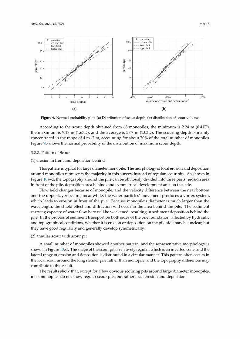
The surveying range is 35 m in the center radius of the monopole. In the center radius of 17 m~35 m,the topographic fluctuation changes are very small (<1 m), and the average altitude is very close to theoriginal designed mudline altitude (<0.1 m). The erosion or deposition are mainly concentrated in therange of 17 m from the center radius of monopile foundations, about 3D. The volume varies between−4307 m3 and 199 m3, and the average value is −1983 m3. Except for the positive values of pile 7# and65#, that is, deposition, the value of other monopile foundations is negative, that is, erosion. Figure 9ais the normal probability plot of erosion and deposition volume.

Appl. Sci. 2020, 10, 7579 9 of 18


165 degrees, and the sounding resolution is 6 mm. SeaBat T50-P multibeam sounding system is

shown in Figure 8b.

3.2. Scour Characteristics

3.2.1. Range of Scour

The surveying range is 35 m in the center radius of the monopole. In the center radius of 17

m~35 m, the topographic fluctuation changes are very small (<1 m), and the average altitude is very

close to the original designed mudline altitude (<0.1 m). The erosion or deposition are mainly

concentrated in the range of 17 m from the center radius of monopile foundations, about 3D. The

volume varies between −4307 m3 and 199 m3, and the average value is −1983 m3. Except for the

positive values of pile 7# and 65#, that is, deposition, the value of other monopile foundations is

negative, that is, erosion. Figure 9a is the normal probability plot of erosion and deposition volume.

1 2 3 4 5 6 7 8 9 10

1

10

40

70

95

99.5

perc

enta

ge

scour depth/m

percentile

reference line

lowerlimit

higher limit

-6000 -4000 -2000 0 2000

1

10

40

70

95

99.5

volume of erosion and deposition/m3

per

cen

tag

e

percentile

reference line

lower limit

upper limit

(a) (b)

Figure 9. Normal probability plot. (a) Distribution of scour depth; (b) distribution of scour volume.

According to the scour depth obtained from 68 monopiles, the minimum is 2.24 m (0.41D), the

maximum is 9.18 m (1.67D), and the average is 5.67 m (1.03D). The scouring depth is mainly

concentrated in the range of 4 m~7 m, accounting for about 70% of the total number of monopiles.

Figure 9b shows the normal probability of the distribution of maximum scour depth.

3.2.2. Pattern of Scour

(1) erosion in front and deposition behind

This pattern is typical for large diameter monopile. The morphology of local erosion and

deposition around monopiles represents the majority in this survey, instead of regular scour pits.

As shown in Figure 10a–d, the topography around the pile can be obviously divided into three

parts: erosion area in front of the pile, deposition area behind, and symmetrical development area

on the side.

Figure 9. Normal probability plot. (a) Distribution of scour depth; (b) distribution of scour volume.

According to the scour depth obtained from 68 monopiles, the minimum is 2.24 m (0.41D),the maximum is 9.18 m (1.67D), and the average is 5.67 m (1.03D). The scouring depth is mainlyconcentrated in the range of 4 m~7 m, accounting for about 70% of the total number of monopiles.Figure 9b shows the normal probability of the distribution of maximum scour depth.

3.2.2. Pattern of Scour

(1) erosion in front and deposition behind

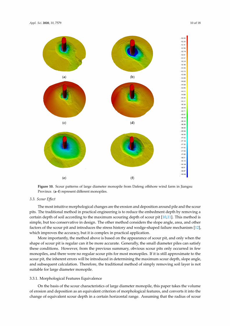
This pattern is typical for large diameter monopile. The morphology of local erosion and depositionaround monopiles represents the majority in this survey, instead of regular scour pits. As shown inFigure 10a–d, the topography around the pile can be obviously divided into three parts: erosion areain front of the pile, deposition area behind, and symmetrical development area on the side.

Flow field changes because of monopile, and the velocity difference between the near bottomand the upper layer occurs; meanwhile, the water particles’ movement produces a vortex system,which leads to erosion in front of the pile. Because monopile’s diameter is much larger than thewavelength, the shield effect and diffraction will occur in the area behind the pile. The sedimentcarrying capacity of water flow here will be weakened, resulting in sediment deposition behind thepile. In the process of sediment transport on both sides of the pile foundation, affected by hydraulicand topographical conditions, whether it is erosion or deposition on the pile side may be unclear, butthey have good regularity and generally develop symmetrically.

(2) annular scour with scour pit

A small number of monopiles showed another pattern, and the representative morphology isshown in Figure 10e,f. The shape of the scour pit is relatively regular, which is an inverted cone, and thelateral range of erosion and deposition is distributed in a circular manner. This pattern often occurs inthe local scour around the long slender pile rather than monopile, and the topography differences maycontribute to this result.

The results show that, except for a few obvious scouring pits around large diameter monopiles,most monopiles do not show regular scour pits, but rather local erosion and deposition.

Appl. Sci. 2020, 10, 7579 10 of 18Appl. Sci. 2020, 10, x FOR PEER REVIEW 10 of 19

(a) (b)

(c) (d)

(e) (f)

Figure 10. Scour patterns of large diameter monopile from Dafeng offshore wind farm in Jiangsu Province. (a–f) represent different monopiles.

Flow field changes because of monopile, and the velocity difference between the near bottom and the upper layer occurs; meanwhile, the water particles’ movement produces a vortex system, which leads to erosion in front of the pile. Because monopile’s diameter is much larger than the wavelength, the shield effect and diffraction will occur in the area behind the pile. The sediment carrying capacity of water flow here will be weakened, resulting in sediment deposition behind the pile. In the process of sediment transport on both sides of the pile foundation, affected by hydraulic and topographical conditions, whether it is erosion or deposition on the pile side may be unclear, but they have good regularity and generally develop symmetrically.

(2) annular scour with scour pit

A small number of monopiles showed another pattern, and the representative morphology is shown in Figure 10e,f. The shape of the scour pit is relatively regular, which is an inverted cone, and the lateral range of erosion and deposition is distributed in a circular manner. This pattern often occurs in the local scour around the long slender pile rather than monopile, and the topography differences may contribute to this result.

The results show that, except for a few obvious scouring pits around large diameter monopiles, most monopiles do not show regular scour pits, but rather local erosion and deposition.

3.3. Scour Effect

The most intuitive morphological changes are the erosion and deposition around pile and the scour pits. The traditional method in practical engineering is to reduce the embedment depth by

Figure 10. Scour patterns of large diameter monopile from Dafeng offshore wind farm in JiangsuProvince. (a–f) represent different monopiles.

3.3. Scour Effect

The most intuitive morphological changes are the erosion and deposition around pile and the scourpits. The traditional method in practical engineering is to reduce the embedment depth by removing acertain depth of soil according to the maximum scouring depth of scour pit [10,11]. This method issimple, but too conservative in design. The other method considers the slope angle, area, and otherfactors of the scour pit and introduces the stress history and wedge-shaped failure mechanism [12],which improves the accuracy, but it is complex in practical application.

More importantly, the method above is based on the appearance of scour pit, and only when theshape of scour pit is regular can it be more accurate. Generally, the small diameter piles can satisfythese conditions. However, from the previous summary, obvious scour pits only occurred in fewmonopiles, and there were no regular scour pits for most monopiles. If it is still approximate to thescour pit, the inherent errors will be introduced in determining the maximum scour depth, slope angle,and subsequent calculation. Therefore, the traditional method of simply removing soil layer is notsuitable for large diameter monopile.

3.3.1. Morphological Features Equivalence

On the basis of the scour characteristics of large diameter monopile, this paper takes the volumeof erosion and deposition as an equivalent criterion of morphological features, and converts it into thechange of equivalent scour depth in a certain horizontal range. Assuming that the radius of scour

Appl. Sci. 2020, 10, 7579 11 of 18

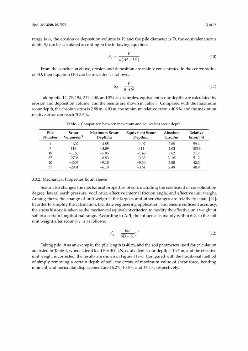
range is A, the erosion or deposition volume is V, and the pile diameter is D, the equivalent scourdepth Sd can be calculated according to the following equation:

Sd =V

π(A2 −D2)(10)

From the conclusion above, erosion and deposition are mainly concentrated in the center radiusof 3D, then Equation (10) can be rewritten as follows:

Sd =V

8πD2 (11)

Taking pile 1#, 7#, 19#, 37#, 40#, and 57# as examples, equivalent scour depths are calculated byerosion and deposition volume, and the results are shown in Table 3. Compared with the maximumscour depth, the absolute error is 2.88 m~4.03 m, the minimum relative error is 40.9%, and the maximumrelative error can reach 103.6%.

Table 3. Comparison between maximum and equivalent scour depth.

PileNumber

ScourVolume/m3

Maximum ScourDepth/m

Equivalent ScourDepth/m

AbsoluteError/m

RelativeError/(%)

1 −1602 −4.85 −1.97 2.88 59.47 113 −3.89 0.14 4.03 103.6

19 −1163 −5.05 −1.48 3.62 71.737 −2708 −6.83 −3.33 3. 05 51.240 −4307 −9.18 −5.30 3.88 42.357 −2931 −6.10 −3.61 2.49 40.9

3.3.2. Mechanical Properties Equivalence

Scour also changes the mechanical properties of soil, including the coefficient of consolidationdegree, lateral earth pressure, void ratio, effective internal friction angle, and effective unit weight.Among them, the change of unit weigh is the largest, and other changes are relatively small [24].In order to simplify the calculation, facilitate engineering application, and ensure sufficient accuracy,the stress history is taken as the mechanical equivalent criterion to modify the effective unit weight ofsoil in a certain longitudinal range. According to API, the influence is mainly within 6D, so the soilunit weight after scour γ′sc is as follows:

γ′sc =6D

6D− Sdγ′ (12)

Taking pile 1# as an example, the pile length is 40 m, and the soil parameters used for calculationare listed in Table 4, where lateral load F = 400 kN, equivalent scour depth is 1.97 m, and the effectiveunit weight is corrected; the results are shown in Figure 11a–c. Compared with the traditional methodof simply removing a certain depth of soil, the errors of maximum value of shear force, bendingmoment, and horizontal displacement are 16.2%, 10.6%, and 46.4%, respectively.

Appl. Sci. 2020, 10, 7579 12 of 18

Table 4. Soil parameters of the construction site.

Soil LayerNumber Soil Name Depth/m Effective Unit

Weight/(kN/m2)Friction

Angle/() Cohesion/kPa

1 Clay 0–2.4 7.6 2.3 4.52 Medium sand 2.4–6.1 8.1 23 03 Clay 6.1–15.9 7.8 3.5 9.74 Medium coarse sand 15.9–19.8 8.5 23 05 Sandy clay 19.8–21.4 9.3 13 306 Silty clay 21.4- 10.5 26 25


6' '6sc

d

DD S

γ γ=−

(12)

Taking pile 1# as an example, the pile length is 40 m, and the soil parameters used for calculation are listed in Table 4, where lateral load F = 400 kN, equivalent scour depth is 1.97 m, and the effective unit weight is corrected; the results are shown in Figure 11a–c. Compared with the traditional method of simply removing a certain depth of soil, the errors of maximum value of shear force, bending moment, and horizontal displacement are 16.2%, 10.6%, and 46.4%, respectively.

Table 4. Soil parameters of the construction site.

Soil Layer Number

Soil Name Depth/m Effective Unit Weight/(kN/m2)

Friction Angle/(°)

Cohesion/kPa

1 Clay 0–2.4 7.6 2.3 4.5 2 Medium sand 2.4–6.1 8.1 23 0 3 Clay 6.1–15.9 7.8 3.5 9.7

4 Medium coarse sand 15.9–19.8 8.5 23 0

5 Sandy clay 19.8–21.4 9.3 13 30 6 Silty clay 21.4- 10.5 26 25

40

35

30

25

20

15

10

5

0-1200 -1000 -800 -600 -400 -200 0 200 400

shear /kN

dept

h/m

without scour traditional method method in this paper

40

35

30

25

20

15

10

5

00 2000 4000 6000 8000


moment/kN•mde

pth/

m

40

35

30

25

20

15

10

5

0-4 -2 0 2 4 6 8 10 12 14 16 18 20


horizontal displacement/mm

dept

h/m

(a) (b) (c)

Figure 11. Deformation response calculated by different methods. (a) Shear force; (b) bending moment. (c) horizontal displacement.

4. Displacement of Large Diameter Monopile under Scour

The numerical analysis was verified in Section 2, and the scour effect was quantified in Section 3. By the proposed frame, on the basis of the data below, a finite element model was established in ABAQUS. The p–y curves for large diameter monopiles considering scour effect were obtained and then used to displacement analysis on large diameter monopiles under scour.

4.1. Model Parameters

The soil parameters in the construction site are shown in Table 4. The total length of the pile shaft is 40 m, and the embedment depth is 30 m. The outside diameter is 4 m and the wall thickness is 100 mm [25].

Zhang et al. [5] have verified that the isotropic hardening model can accurately predict the stress–strain behavior of saturated soil, so the Mises yield criterion and isotropic hardening model are adopted in this study. The initial and limiting yield stress were obtained by tri-axial CU test, and 15 sets of subsequent yield stress and corresponding strain were imported to ABAQUS to

Figure 11. Deformation response calculated by different methods. (a) Shear force; (b) bending moment.(c) horizontal displacement.

4. Displacement of Large Diameter Monopile under Scour

The numerical analysis was verified in Section 2, and the scour effect was quantified in Section 3.By the proposed frame, on the basis of the data below, a finite element model was established inABAQUS. The p–y curves for large diameter monopiles considering scour effect were obtained andthen used to displacement analysis on large diameter monopiles under scour.

4.1. Model Parameters

The soil parameters in the construction site are shown in Table 4. The total length of the pile shaftis 40 m, and the embedment depth is 30 m. The outside diameter is 4 m and the wall thickness is100 mm [25].

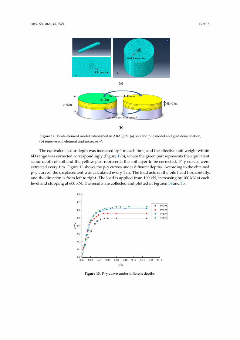
Zhang et al. [5] have verified that the isotropic hardening model can accurately predict thestress–strain behavior of saturated soil, so the Mises yield criterion and isotropic hardening modelare adopted in this study. The initial and limiting yield stress were obtained by tri-axial CU test,and 15 sets of subsequent yield stress and corresponding strain were imported to ABAQUS to describethe strain-hardening in the stage of plastic. The three-dimensional model is meshed by eight-nodehexahedron element and reduced integration and hourglass control is used in the analysis. A surfaceto surface interaction is created to simulate the pile–soil interaction. To avoid the boundary conditioneffect, the soil is 160 m in diameter and 60 m in height. The soil and pile interaction surface wasidealized as frictionless. The grid within 24 m of monopile foundation is densified. The finite elementmodel is shown in Figure 12a.

Appl. Sci. 2020, 10, 7579 13 of 18


describe the strain-hardening in the stage of plastic. The three-dimensional model is meshed by eight-node hexahedron element and reduced integration and hourglass control is used in the analysis. A surface to surface interaction is created to simulate the pile–soil interaction. To avoid the boundary condition effect, the soil is 160 m in diameter and 60 m in height. The soil and pile interaction surface was idealized as frictionless. The grid within 24 m of monopile foundation is densified. The finite element model is shown in Figure 12a.

(a)

(b)

Figure 12. Finite element model established in ABAQUS. (a) Soil and pile model and grid densification; (b) remove soil element and increase γ’.

The equivalent scour depth was increased by 1 m each time, and the effective unit weight within 6D range was corrected correspondingly (Figure 12b), where the green part represents the equivalent scour depth of soil and the yellow part represents the soil layer to be corrected. P–y curves were extracted every 1 m. Figure 13 shows the p–y curves under different depths. According to the obtained p–y curves, the displacement was calculated every 1 m. The load acts on the pile head horizontally, and the direction is from left to right. The load is applied from 100 kN, increasing by 100 kN at each level and stopping at 600 kN. The results are collected and plotted in Figures 14 and 15.

Figure 12. Finite element model established in ABAQUS. (a) Soil and pile model and grid densification;(b) remove soil element and increase γ’.

The equivalent scour depth was increased by 1 m each time, and the effective unit weight within6D range was corrected correspondingly (Figure 12b), where the green part represents the equivalentscour depth of soil and the yellow part represents the soil layer to be corrected. P–y curves wereextracted every 1 m. Figure 13 shows the p–y curves under different depths. According to the obtainedp–y curves, the displacement was calculated every 1 m. The load acts on the pile head horizontally,and the direction is from left to right. The load is applied from 100 kN, increasing by 100 kN at eachlevel and stopping at 600 kN. The results are collected and plotted in Figures 14 and 15.


Figure 13. P–y curve under different depths.

0 100 200 300 400 500 6000

2

4

6

8

10

12

14

16

18

20

norm

aliz

ed p

ile h

ead

disp

lace

men

t y/D

/10-3

load /kN

without scour Sd=0.5D Sd=1D Sd=1.5D

(a) (b)

Figure 14. Pile head displacement of monopile under scour. (a) Scour depth–displacement under different load levels; (b) load–displacement under different scour depths.

Figure 15. Scour depth–apparent fixity depth under different load levels.

4.2. Discussion

0.00 0.02 0.04 0.06 0.08 0.10 0.12 0.14 0.16 0.180.0

0.1

0.2

0.3

0.4

0.5

0.6

0.7

0.8

p/p u

y/D

z=2m z=4m z=6m z=8m

0.0 0.5 1.0 1.5 2.0 2.50

2

4

6

8

10

12

14

16

norm

aliz

ed d

ispla

cem

ent y

/D /1

0-3

scour depth Sd/D

F=100kN F=200kN F=300kN F=400kN

0.0 0.5 1.0 1.5 2.0 2.58.1

8.2

8.3

8.4

8.5

8.6

8.7

8.8

dept

h of

app

aren

t fix

ity p

oint

z/D

scour depth y/D

200 kN 400 kN 600 kN


Appl. Sci. 2020, 10, 7579 14 of 18



0 100 200 300 400 500 6000

2

4

6

8

10

12

14

16

18

20

norm

aliz

ed p

ile h

ead

disp

lace

men

t y/D

/10-3

load /kN


(a) (b)



4.2. Discussion

0.00 0.02 0.04 0.06 0.08 0.10 0.12 0.14 0.16 0.180.0

0.1

0.2

0.3

0.4

0.5

0.6

0.7

0.8

p/p u

y/D

z=2m z=4m z=6m z=8m

0.0 0.5 1.0 1.5 2.0 2.50

2

4

6

8

10

12

14

16

norm

aliz

ed d

ispla

cem

ent y

/D /1

0-3

scour depth Sd/D

F=100kN F=200kN F=300kN F=400kN

0.0 0.5 1.0 1.5 2.0 2.58.1

8.2

8.3

8.4

8.5

8.6

8.7

8.8

dept

h of

app

aren

t fix

ity p

oint

z/D

scour depth y/D

200 kN 400 kN 600 kN

Figure 14. Pile head displacement of monopile under scour. (a) Scour depth–displacement underdifferent load levels; (b) load–displacement under different scour depths.



0 100 200 300 400 500 6000

2

4

6

8

10

12

14

16

18

20

norm

aliz

ed p

ile h

ead

disp

lace

men

t y/D

/10-3

load /kN


(a) (b)



4.2. Discussion

0.00 0.02 0.04 0.06 0.08 0.10 0.12 0.14 0.16 0.180.0

0.1

0.2

0.3

0.4

0.5

0.6

0.7

0.8

p/p u

y/D

z=2m z=4m z=6m z=8m

0.0 0.5 1.0 1.5 2.0 2.50

2

4

6

8

10

12

14

16

norm

aliz

ed d

ispla

cem

ent y

/D /1

0-3

scour depth Sd/D

F=100kN F=200kN F=300kN F=400kN

0.0 0.5 1.0 1.5 2.0 2.58.1

8.2

8.3

8.4

8.5

8.6

8.7

8.8

dept

h of

app

aren

t fix

ity p

oint

z/D

scour depth y/D

200 kN 400 kN 600 kN


4.2. Discussion

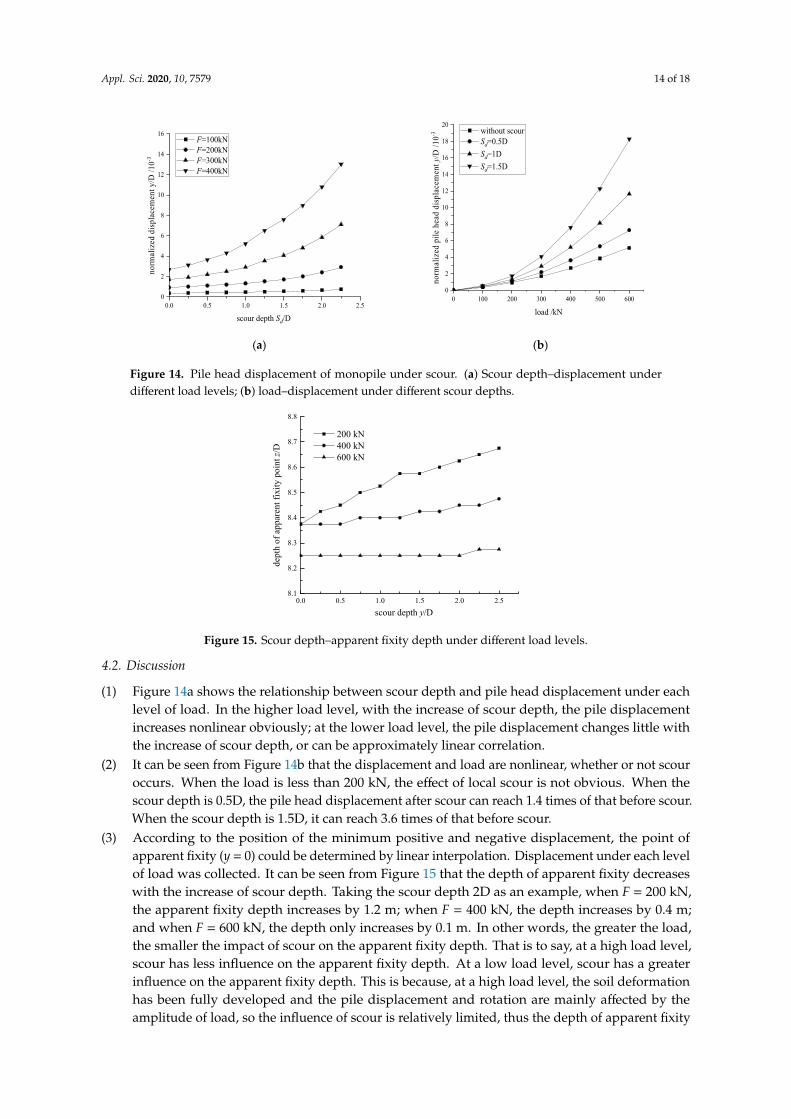
(1) Figure 14a shows the relationship between scour depth and pile head displacement under eachlevel of load. In the higher load level, with the increase of scour depth, the pile displacementincreases nonlinear obviously; at the lower load level, the pile displacement changes little withthe increase of scour depth, or can be approximately linear correlation.

(2) It can be seen from Figure 14b that the displacement and load are nonlinear, whether or not scouroccurs. When the load is less than 200 kN, the effect of local scour is not obvious. When thescour depth is 0.5D, the pile head displacement after scour can reach 1.4 times of that before scour.When the scour depth is 1.5D, it can reach 3.6 times of that before scour.

(3) According to the position of the minimum positive and negative displacement, the point ofapparent fixity (y = 0) could be determined by linear interpolation. Displacement under each levelof load was collected. It can be seen from Figure 15 that the depth of apparent fixity decreaseswith the increase of scour depth. Taking the scour depth 2D as an example, when F = 200 kN,the apparent fixity depth increases by 1.2 m; when F = 400 kN, the depth increases by 0.4 m;and when F = 600 kN, the depth only increases by 0.1 m. In other words, the greater the load,the smaller the impact of scour on the apparent fixity depth. That is to say, at a high load level,scour has less influence on the apparent fixity depth. At a low load level, scour has a greaterinfluence on the apparent fixity depth. This is because, at a high load level, the soil deformationhas been fully developed and the pile displacement and rotation are mainly affected by theamplitude of load, so the influence of scour is relatively limited, thus the depth of apparent fixity

Appl. Sci. 2020, 10, 7579 15 of 18

has no obvious change under scour. Meanwhile, at a low load level, the soil deformation is small,and scour deteriorates the soil conditions and reduces the embedment depth; thus, comparedwith load amplitude, scour also has a great influence on the depth of the apparent fixity.

5. Sensitivity of Pile Head Displacement under Scour

The increase of pile diameter, embedment length, and wall thickness can reduce the displacementof monopiles, but the variation characteristics under scour are not clear. For example, the horizontaldisplacement can be reduced by altering a certain pile parameter, but its effect may be greatly reducedunder scour, which decreases the economy and safety of monopile foundations. Therefore, in thissection, by discussing the relationships between pile head displacement, pile parameters, and scourdepth, the sensitivity of displacement under scour is studied. This is how the analysis is realized:keeping the scour depth fixed to study the relationship between pile head displacement and pileparameters; and keeping the pile parameters fixed to study the displacement before and after scouring.To quantify the variation extent of horizontal displacement before and after scouring, the concept ofscour sensitivity S is defined, which takes displacement as reference:

S =dt

d0(13)

The value of S represents the susceptibility to scour. A higher value of S indicates a larger ratio ofdisplacement after scour than that before scour, and that the parameter studied is more susceptible toscour. In the same way, a lower value of S indicates a smaller ratio of displacement after scour to thatbefore scour, and that the parameter studied is less susceptible to scour.

According to Section 3, the average scour depth is 1.03D, and in order to facilitate the comparison,all scour depths in this section are taken as 1D. The initial pile diameter, embedment length, and wallthickness are 4 m, 40 m, and 100 mm, respectively. The value of pile parameters increases by 50% fromthe initial value, and the changes of displacement and scour sensitivity of pile head are compared.The load is applied to the top of the pile, with the amplitude of 600 kN and the direction from leftto right.

5.1. Pile Diameter

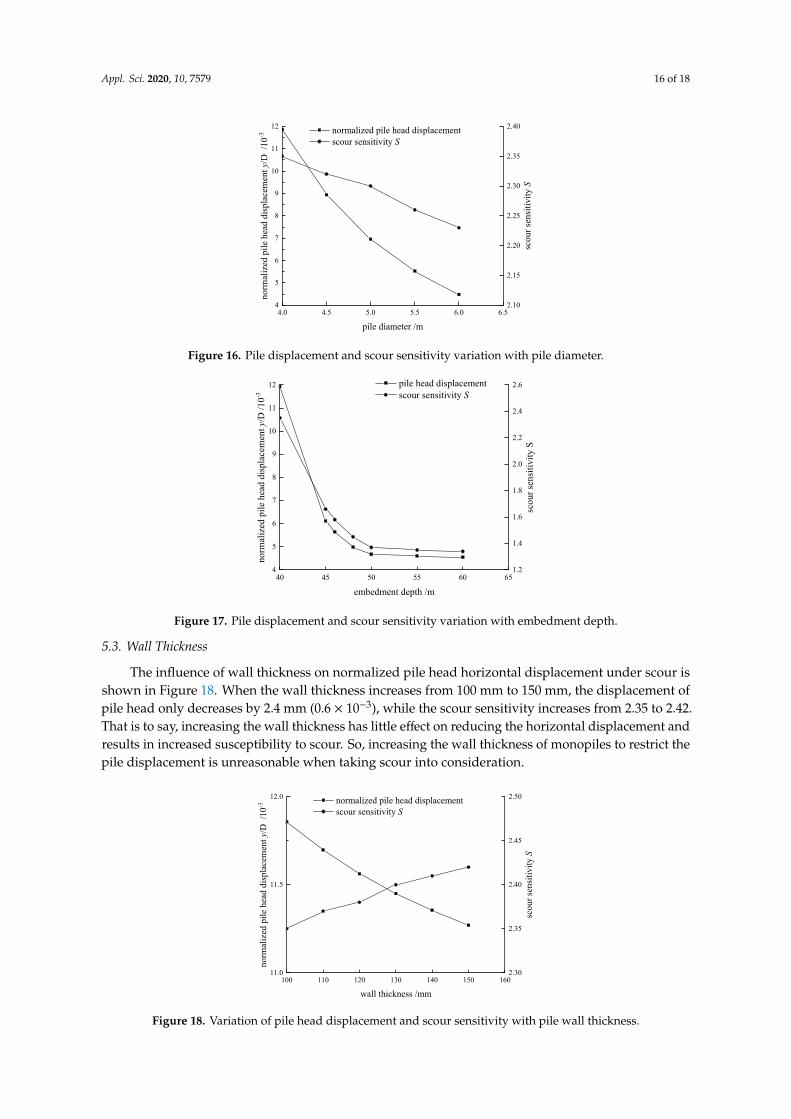
The pile length and wall thickness of large diameter monopile is fixed, and the pile diametersof 4, 4.5, 5, 5.5, and 6 m are input in sequence. When the pile diameter increases from 4 m to 6 m,the horizontal displacement of pile head decreases from 47.7 mm (11.925 × 10−3) to 26.9 mm (6.725 ×10−3), which is 58% of the original value. The scour sensitivity decreased slightly from 2.35 to 2.23.The normalized displacement and sensitivity of pile head calculated under different pile diameters areshown in Figure 16. This illustrates that increasing the pile diameter will reduce the pile displacement,and the susceptibility to scour decreases slightly.

5.2. Pile Length

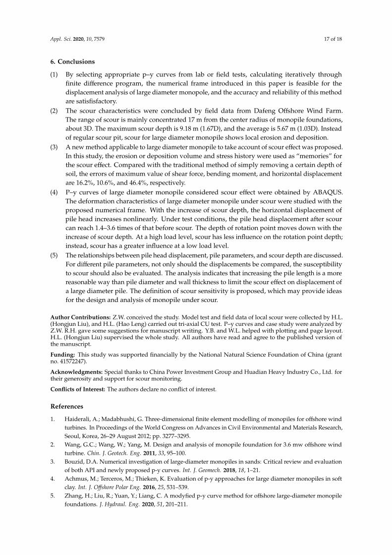
Figure 17 shows the normalized horizontal displacement and scour sensitivity of pile head underdifferent pile lengths. The length of pile increases from 40 m to 60 m; the normalized horizontaldisplacement of pile head decreases from 11.925 × 10−3 (47.7 mm) to 4.55 × 10−3 (18.2 mm), becoming38% of the original; and the scour sensitivity decreases from 2.35 to 1.34. It can be seen that increasingthe pile length can significantly reduce the horizontal displacement of the pile body, and at the sametime, the scouring sensitivity is also greatly reduced, which means the displacements are affected byscour to a lesser extent.

When the pile length reaches 50 m, the pile head displacement is 4.675 × 10−3, and the scoursensitivity S is 1.37. After that, increasing the pile length will not lead to an obvious change of horizontaldisplacement and scour sensitivity, so it could be considered as a critical value.

Appl. Sci. 2020, 10, 7579 16 of 18


the horizontal displacement of pile head decreases from 47.7 mm (11.925 × 10−3) to 26.9 mm (6.725 × 10−3), which is 58% of the original value. The scour sensitivity decreased slightly from 2.35 to 2.23. The normalized displacement and sensitivity of pile head calculated under different pile diameters are shown in Figure 16. This illustrates that increasing the pile diameter will reduce the pile displacement, and the susceptibility to scour decreases slightly.

Figure 16. Pile displacement and scour sensitivity variation with pile diameter.

5.2. Pile Length

Figure 17 shows the normalized horizontal displacement and scour sensitivity of pile head under different pile lengths. The length of pile increases from 40 m to 60 m; the normalized horizontal displacement of pile head decreases from 11.925 × 10−3 (47.7 mm) to 4.55 × 10−3 (18.2 mm), becoming 38% of the original; and the scour sensitivity decreases from 2.35 to 1.34. It can be seen that increasing the pile length can significantly reduce the horizontal displacement of the pile body, and at the same time, the scouring sensitivity is also greatly reduced, which means the displacements are affected by scour to a lesser extent.

Figure 17. Pile displacement and scour sensitivity variation with embedment depth.

When the pile length reaches 50 m, the pile head displacement is 4.675 × 10−3, and the scour sensitivity S is 1.37. After that, increasing the pile length will not lead to an obvious change of horizontal displacement and scour sensitivity, so it could be considered as a critical value.

5.3. Wall Thickness

4.0 4.5 5.0 5.5 6.0 6.54

5

6

7

8

9

10

11

12

norm

aliz

ed p

ile h

ead

disp

lace

men

t y/D

/10

-3

pile diameter /m

normalized pile head displacement scour sensitivity S

2.10

2.15

2.20

2.25

2.30

2.35

2.40

scou

r sen

sitiv

ity S

40 45 50 55 60 654

5

6

7

8

9

10

11

12

norm

aliz

ed p

ile h

ead

disp

lace

men

t y/D

/10-3

embedment depth /m

pile head displacement scour sensitivity S

1.2

1.4

1.6

1.8

2.0

2.2

2.4

2.6

scou

r sen

sitiv

ity S



the horizontal displacement of pile head decreases from 47.7 mm (11.925 × 10−3) to 26.9 mm (6.725 × 10−3), which is 58% of the original value. The scour sensitivity decreased slightly from 2.35 to 2.23. The normalized displacement and sensitivity of pile head calculated under different pile diameters are shown in Figure 16. This illustrates that increasing the pile diameter will reduce the pile displacement, and the susceptibility to scour decreases slightly.


5.2. Pile Length

Figure 17 shows the normalized horizontal displacement and scour sensitivity of pile head under different pile lengths. The length of pile increases from 40 m to 60 m; the normalized horizontal displacement of pile head decreases from 11.925 × 10−3 (47.7 mm) to 4.55 × 10−3 (18.2 mm), becoming 38% of the original; and the scour sensitivity decreases from 2.35 to 1.34. It can be seen that increasing the pile length can significantly reduce the horizontal displacement of the pile body, and at the same time, the scouring sensitivity is also greatly reduced, which means the displacements are affected by scour to a lesser extent.


When the pile length reaches 50 m, the pile head displacement is 4.675 × 10−3, and the scour sensitivity S is 1.37. After that, increasing the pile length will not lead to an obvious change of horizontal displacement and scour sensitivity, so it could be considered as a critical value.

5.3. Wall Thickness

4.0 4.5 5.0 5.5 6.0 6.54

5

6

7

8

9

10

11

12

norm

aliz

ed p

ile h

ead

disp

lace

men

t y/D

/10

-3

pile diameter /m


2.10

2.15

2.20

2.25

2.30

2.35

2.40

scou

r sen

sitiv

ity S

40 45 50 55 60 654

5

6

7

8

9

10

11

12

norm

aliz

ed p

ile h

ead

disp

lace

men

t y/D

/10-3

embedment depth /m

pile head displacement scour sensitivity S

1.2

1.4

1.6

1.8

2.0

2.2

2.4

2.6

scou

r sen

sitiv

ity S


5.3. Wall Thickness

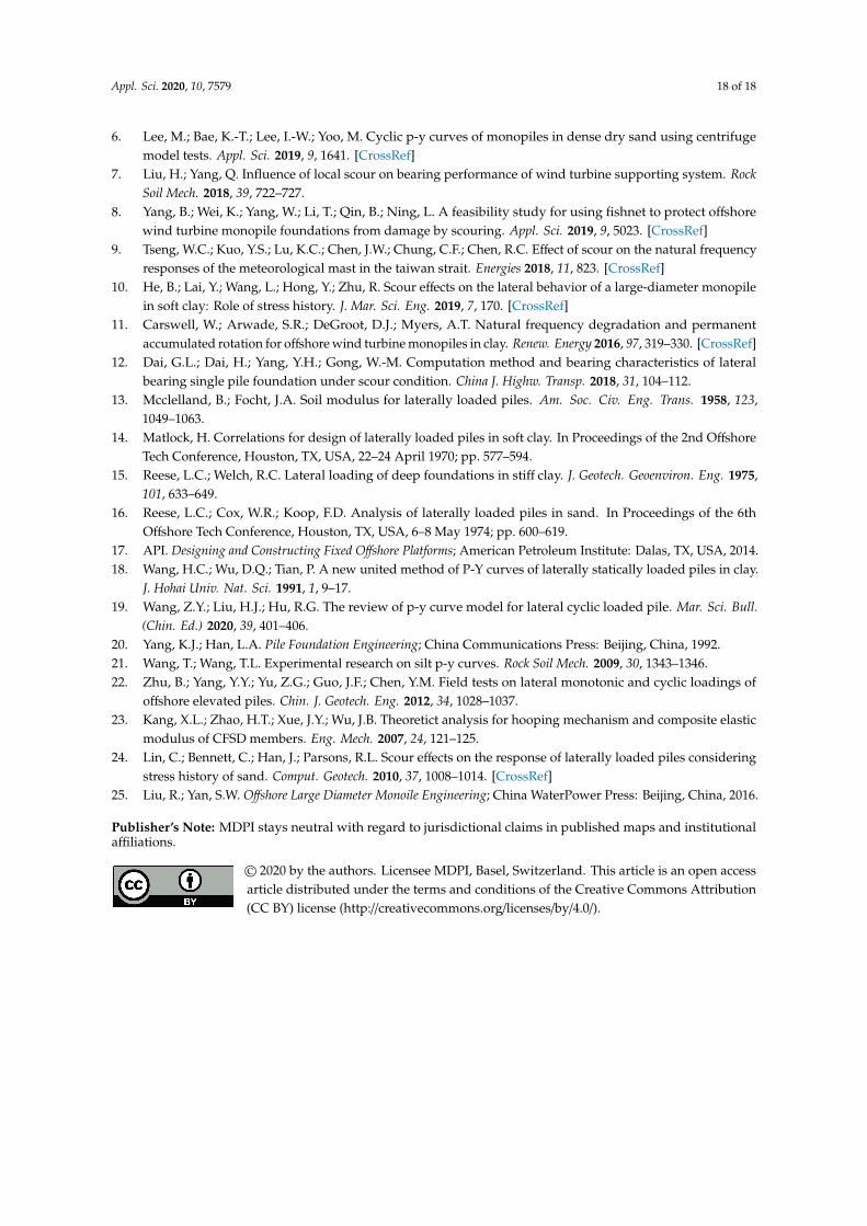
The influence of wall thickness on normalized pile head horizontal displacement under scour isshown in Figure 18. When the wall thickness increases from 100 mm to 150 mm, the displacement ofpile head only decreases by 2.4 mm (0.6 × 10−3), while the scour sensitivity increases from 2.35 to 2.42.That is to say, increasing the wall thickness has little effect on reducing the horizontal displacement andresults in increased susceptibility to scour. So, increasing the wall thickness of monopiles to restrict thepile displacement is unreasonable when taking scour into consideration.


The influence of wall thickness on normalized pile head horizontal displacement under scour is shown in Figure 18. When the wall thickness increases from 100 mm to 150 mm, the displacement of pile head only decreases by 2.4 mm (0.6 × 10−3), while the scour sensitivity increases from 2.35 to 2.42. That is to say, increasing the wall thickness has little effect on reducing the horizontal displacement and results in increased susceptibility to scour. So, increasing the wall thickness of monopiles to restrict the pile displacement is unreasonable when taking scour into consideration.

Figure 18. Variation of pile head displacement and scour sensitivity with pile wall thickness.

6. Conclusions

(1) By selecting appropriate p–y curves from lab or field tests, calculating iteratively through finite difference program, the numerical frame introduced in this paper is feasible for the displacement analysis of large diameter monopole, and the accuracy and reliability of this method are satisfisfactory.

(2) The scour characteristics were concluded by field data from Dafeng Offshore Wind Farm. The range of scour is mainly concentrated 17 m from the center radius of monopile foundations, about 3D. The maximum scour depth is 9.18 m (1.67D), and the average is 5.67 m (1.03D). Instead of regular scour pit, scour for large diameter monopile shows local erosion and deposition.

(3) A new method applicable to large diameter monopile to take account of scour effect was proposed. In this study, the erosion or deposition volume and stress history were used as “memories” for the scour effect. Compared with the traditional method of simply removing a certain depth of soil, the errors of maximum value of shear force, bending moment, and horizontal displacement are 16.2%, 10.6%, and 46.4%, respectively.

(4) P–y curves of large diameter monopile considered scour effect were obtained by ABAQUS. The deformation characteristics of large diameter monopile under scour were studied with the proposed numerical frame. With the increase of scour depth, the horizontal displacement of pile head increases nonlinearly. Under test conditions, the pile head displacement after scour can reach 1.4–3.6 times of that before scour. The depth of rotation point moves down with the increase of scour depth. At a high load level, scour has less influence on the rotation point depth; instead, scour has a greater influence at a low load level.

(5) The relationships between pile head displacement, pile parameters, and scour depth are discussed. For different pile parameters, not only should the displacements be compared, the susceptibility to scour should also be evaluated. The analysis indicates that increasing the pile length is a more reasonable way than pile diameter and wall thickness to limit the scour effect on displacement of a large diameter pile. The definition of scour sensitivity is proposed, which may provide ideas for the design and analysis of monopile under scour.

Author Contributions: Z.W. conceived the study. Model test and field data of local scour were collected by H.L. (Hongjun Liu), and H.L. (Hao Leng) carried out tri-axial CU test. P–y curves and case study were

100 110 120 130 140 150 16011.0

11.5

12.0

norm

aliz

ed p

ile h

ead

disp

lace

men

t y/D

/10

-3

wall thickness /mm


2.30

2.35

2.40

2.45

2.50

scou

r sen

sitiv

ity S

Figure 18. Variation of pile head displacement and scour sensitivity with pile wall thickness.

Appl. Sci. 2020, 10, 7579 17 of 18

6. Conclusions

(1) By selecting appropriate p–y curves from lab or field tests, calculating iteratively throughfinite difference program, the numerical frame introduced in this paper is feasible for thedisplacement analysis of large diameter monopole, and the accuracy and reliability of this methodare satisfisfactory.

(2) The scour characteristics were concluded by field data from Dafeng Offshore Wind Farm.The range of scour is mainly concentrated 17 m from the center radius of monopile foundations,about 3D. The maximum scour depth is 9.18 m (1.67D), and the average is 5.67 m (1.03D). Insteadof regular scour pit, scour for large diameter monopile shows local erosion and deposition.

(3) A new method applicable to large diameter monopile to take account of scour effect was proposed.In this study, the erosion or deposition volume and stress history were used as “memories” forthe scour effect. Compared with the traditional method of simply removing a certain depth ofsoil, the errors of maximum value of shear force, bending moment, and horizontal displacementare 16.2%, 10.6%, and 46.4%, respectively.

(4) P–y curves of large diameter monopile considered scour effect were obtained by ABAQUS.The deformation characteristics of large diameter monopile under scour were studied with theproposed numerical frame. With the increase of scour depth, the horizontal displacement ofpile head increases nonlinearly. Under test conditions, the pile head displacement after scourcan reach 1.4–3.6 times of that before scour. The depth of rotation point moves down with theincrease of scour depth. At a high load level, scour has less influence on the rotation point depth;instead, scour has a greater influence at a low load level.

(5) The relationships between pile head displacement, pile parameters, and scour depth are discussed.For different pile parameters, not only should the displacements be compared, the susceptibilityto scour should also be evaluated. The analysis indicates that increasing the pile length is a morereasonable way than pile diameter and wall thickness to limit the scour effect on displacement ofa large diameter pile. The definition of scour sensitivity is proposed, which may provide ideasfor the design and analysis of monopile under scour.

Author Contributions: Z.W. conceived the study. Model test and field data of local scour were collected by H.L.(Hongjun Liu), and H.L. (Hao Leng) carried out tri-axial CU test. P–y curves and case study were analyzed byZ.W. R.H. gave some suggestions for manuscript writing. Y.B. and W.L. helped with plotting and page layout.H.L. (Hongjun Liu) supervised the whole study. All authors have read and agree to the published version ofthe manuscript.

Funding: This study was supported financially by the National Natural Science Foundation of China (grantno. 41572247).

Acknowledgments: Special thanks to China Power Investment Group and Huadian Heavy Industry Co., Ltd. fortheir generosity and support for scour monitoring.

Conflicts of Interest: The authors declare no conflict of interest.

References

1. Haiderali, A.; Madabhushi, G. Three-dimensional finite element modelling of monopiles for offshore windturbines. In Proceedings of the World Congress on Advances in Civil Environmental and Materials Research,Seoul, Korea, 26–29 August 2012; pp. 3277–3295.

2. Wang, G.C.; Wang, W.; Yang, M. Design and analysis of monopile foundation for 3.6 mw offshore windturbine. Chin. J. Geotech. Eng. 2011, 33, 95–100.

3. Bouzid, D.A. Numerical investigation of large-diameter monopiles in sands: Critical review and evaluationof both API and newly proposed p-y curves. Int. J. Geomech. 2018, 18, 1–21.

4. Achmus, M.; Terceros, M.; Thieken, K. Evaluation of p-y approaches for large diameter monopiles in softclay. Int. J. Offshore Polar Eng. 2016, 25, 531–539.

5. Zhang, H.; Liu, R.; Yuan, Y.; Liang, C. A modyfied p-y curve method for offshore large-diameter monopilefoundations. J. Hydraul. Eng. 2020, 51, 201–211.

Appl. Sci. 2020, 10, 7579 18 of 18

6. Lee, M.; Bae, K.-T.; Lee, I.-W.; Yoo, M. Cyclic p-y curves of monopiles in dense dry sand using centrifugemodel tests. Appl. Sci. 2019, 9, 1641. [CrossRef]

7. Liu, H.; Yang, Q. Influence of local scour on bearing performance of wind turbine supporting system. RockSoil Mech. 2018, 39, 722–727.

8. Yang, B.; Wei, K.; Yang, W.; Li, T.; Qin, B.; Ning, L. A feasibility study for using fishnet to protect offshorewind turbine monopile foundations from damage by scouring. Appl. Sci. 2019, 9, 5023. [CrossRef]

9. Tseng, W.C.; Kuo, Y.S.; Lu, K.C.; Chen, J.W.; Chung, C.F.; Chen, R.C. Effect of scour on the natural frequencyresponses of the meteorological mast in the taiwan strait. Energies 2018, 11, 823. [CrossRef]

10. He, B.; Lai, Y.; Wang, L.; Hong, Y.; Zhu, R. Scour effects on the lateral behavior of a large-diameter monopilein soft clay: Role of stress history. J. Mar. Sci. Eng. 2019, 7, 170. [CrossRef]

11. Carswell, W.; Arwade, S.R.; DeGroot, D.J.; Myers, A.T. Natural frequency degradation and permanentaccumulated rotation for offshore wind turbine monopiles in clay. Renew. Energy 2016, 97, 319–330. [CrossRef]

12. Dai, G.L.; Dai, H.; Yang, Y.H.; Gong, W.-M. Computation method and bearing characteristics of lateralbearing single pile foundation under scour condition. China J. Highw. Transp. 2018, 31, 104–112.

13. Mcclelland, B.; Focht, J.A. Soil modulus for laterally loaded piles. Am. Soc. Civ. Eng. Trans. 1958, 123,1049–1063.

14. Matlock, H. Correlations for design of laterally loaded piles in soft clay. In Proceedings of the 2nd OffshoreTech Conference, Houston, TX, USA, 22–24 April 1970; pp. 577–594.

15. Reese, L.C.; Welch, R.C. Lateral loading of deep foundations in stiff clay. J. Geotech. Geoenviron. Eng. 1975,101, 633–649.

16. Reese, L.C.; Cox, W.R.; Koop, F.D. Analysis of laterally loaded piles in sand. In Proceedings of the 6thOffshore Tech Conference, Houston, TX, USA, 6–8 May 1974; pp. 600–619.

17. API. Designing and Constructing Fixed Offshore Platforms; American Petroleum Institute: Dalas, TX, USA, 2014.18. Wang, H.C.; Wu, D.Q.; Tian, P. A new united method of P-Y curves of laterally statically loaded piles in clay.

J. Hohai Univ. Nat. Sci. 1991, 1, 9–17.19. Wang, Z.Y.; Liu, H.J.; Hu, R.G. The review of p-y curve model for lateral cyclic loaded pile. Mar. Sci. Bull.

(Chin. Ed.) 2020, 39, 401–406.20. Yang, K.J.; Han, L.A. Pile Foundation Engineering; China Communications Press: Beijing, China, 1992.21. Wang, T.; Wang, T.L. Experimental research on silt p-y curves. Rock Soil Mech. 2009, 30, 1343–1346.22. Zhu, B.; Yang, Y.Y.; Yu, Z.G.; Guo, J.F.; Chen, Y.M. Field tests on lateral monotonic and cyclic loadings of

offshore elevated piles. Chin. J. Geotech. Eng. 2012, 34, 1028–1037.23. Kang, X.L.; Zhao, H.T.; Xue, J.Y.; Wu, J.B. Theoretict analysis for hooping mechanism and composite elastic

modulus of CFSD members. Eng. Mech. 2007, 24, 121–125.24. Lin, C.; Bennett, C.; Han, J.; Parsons, R.L. Scour effects on the response of laterally loaded piles considering

stress history of sand. Comput. Geotech. 2010, 37, 1008–1014. [CrossRef]25. Liu, R.; Yan, S.W. Offshore Large Diameter Monoile Engineering; China WaterPower Press: Beijing, China, 2016.

Publisher’s Note: MDPI stays neutral with regard to jurisdictional claims in published maps and institutionalaffiliations.

© 2020 by the authors. Licensee MDPI, Basel, Switzerland. This article is an open accessarticle distributed under the terms and conditions of the Creative Commons Attribution(CC BY) license (http://creativecommons.org/licenses/by/4.0/).



http://dx.doi.org/10.3390/en11040823

http://dx.doi.org/10.3390/jmse7060170

http://dx.doi.org/10.1016/j.renene.2016.05.080

http://dx.doi.org/10.1016/j.compgeo.2010.08.009

http://creativecommons.org/

http://creativecommons.org/licenses/by/4.0/.

Documents

Deformation Analysis of Large Diameter Monopiles of