Embed Size (px)
Citation preview
university-logo
Deforming Gravity
L. Pilo1
1Department of PhysicsUniversity of L’Aquila
Cargese 2012
Comelli-Crisostomi-Nesti-LP arXiv:1204.1027 [hep-th]
1 / 22

university-logo
Einstein’s GR
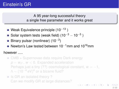
A 95 year-long successful theorya single free parameter and it works great
Weak Equivalence principle (10�13 )Solar system tests (weak field) (10�3 � 10�5 )Binary pulsar (nonlinear) (10�3)Newton’s Law tested between 10�1mm and 1016mm
however .....CMB + Supernovae data require Dark energyp = w⇢ , w < 0. Expanded accelerationPerhaps just a tiny (??) cosmological constant, w = �1,⇤ ⇠ (10�4 eV)4 or a bizarre fluid?Is GR an isolated theory ?Can we modify GR at large distances?
2 / 22

university-logo
Einstein’s GR
A 95 year-long successful theorya single free parameter and it works great
Weak Equivalence principle (10�13 )Solar system tests (weak field) (10�3 � 10�5 )Binary pulsar (nonlinear) (10�3)Newton’s Law tested between 10�1mm and 1016mm
however .....CMB + Supernovae data require Dark energyp = w⇢ , w < 0. Expanded accelerationPerhaps just a tiny (??) cosmological constant, w = �1,⇤ ⇠ (10�4 eV)4 or a bizarre fluid?Is GR an isolated theory ?Can we modify GR at large distances?
2 / 22

university-logo
Massive Deformed GR
Add to GR an extra piece such that when gµ⌫ = ⌘µ⌫ + hµ⌫
(p
g R + Ldef ) = Lspin 2 + m2⇣
a hµ⌫hµ⌫ + b h2⌘
+ · · ·To build a mass term we need an extra tensor field: with gµ⌫ andgµ⌫ there is no non-trivial polynomial of g with no derivativeIntroduce a new tensor field Gµ⌫ , then scalar objects can beconstructed from the metric using
Xµ⌫ = gµ↵G↵⌫ ⌧n = Tr(X n)
Example: G↵⌫ = ⌘↵⌫
gµ⌫Gµ⌫ = 4� hµ⌫⌘µ⌫ + hµ⌫hµ⌫ + · · ·a (⌧1 � 4)2 + b (⌧2 � 2⌧1 + 4) =
⇣a hµ⌫hµ⌫ + b h2
⌘+ · · ·
The metric Gµ⌫ can be dynamical or a priori given: two differentformulations of massive gravity
3 / 22

university-logo
The Stuckelberg Trick in Massive GR
The extra metric is non-dynamical flat given metric
To recover diff (gauge) invariance introduce 4 (Stuckelberg)scalars to recast the fixed metric as
Gµ⌫ =@�A
@xµ
@�B
@x⌫⌘AB
Minimal set of DOF to recover diff invarianceGµ⌫ and Xµ
⌫ transform as tensors and ⌧n = Tr(X n) as scalarsGeometrically �A are coordinates of some fictitious flat space Mpoint-wise identified with the physical spacetime with a tetradbasis eA = d�A
One can chose coordinates such that (Unitary gauge)
@�A
@xµ= �A
µ ) Gµ⌫ = ⌘µ⌫
4 / 22

university-logo
Actions for Massive Gravity
Stuckelberg Formulation
SmGR =
Zd4x
pg M2
pl
hR(g)� 4m2 V (X )
i
Bigravity Formulation
The extra metric Gµ⌫ = gµ⌫ is dynamical
SMGR =
Zd4x M2
pl
hpg R(g) +
pg R(g)� 4 m2pg V (X )
i
When !1, gµ⌫ gets non-dynamical: gµ⌫ = eAµ eB
⌫ ⌘AB
eA = d�A and gµ⌫ = @µ�A@⌫�A ⌘AB
making contact with the Stuckelberg formulation5 / 22

university-logo
Stuckelberg vs Bigravity
The Stuckelberg formulation is minimal, sort of EFT ,The Stuckelberg formulation contains absolute objectsit is an æther-like theory /Fixed flat second metric prevents a spatially flat FRW massivegravity cosmology /Similar troubles with Black Hole (horizon) solutions /Bigravity formulation: all objects are dynamical determined ,No problems with horizons and flat FRW solutions ,The bigravity formulation is more complicated /
From now on we will focus on the Stuckelberg formulation in theunitary gauge
6 / 22

university-logo
Degrees of Freedom: Linear Level
GR M2pl E (1)
µ⌫ = T (1)µ⌫ , gµ⌫ = ⌘µ⌫ + hµ⌫
DOF 10� 2⇥ 4 = 2 4 gauge modes �hµ⌫ = @µ⇠⌫ + @⌫⇠µ
Massive gravitons (Minkowski) have 5 DOF, more DOF neededGive up gauge symmetry. Fierz-Pauli theory (1939)
LFP = M2pl L(2)
spin2 + M2plm
2 �a hµ⌫hµ⌫ + b h2�
E (1)µ⌫ � 1
4m2 (a hµ⌫ + b h ⌘µ⌫) = M�2pl T (1)
µ⌫ @⌫E (1)µ⌫ = 0
4 constraints DOF 10� 4 = 6 = 5 + 1The sixth mode is a ghost (Boulware-Deser).Absent in flat space when a + b = 0 (FP theory)present in curved space and at the non-linear levelWhen the ghost is projected out, light bending badly contradictsexperiments (van Dam, Veltman, Zakharov) vdVZ discontinuity
7 / 22
university-logo
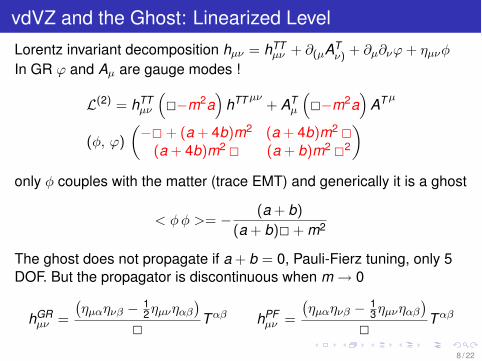
vdVZ and the Ghost: Linearized LevelLorentz invariant decomposition hµ⌫ = hTT
µ⌫ + @(µAT⌫) + @µ@⌫' + ⌘µ⌫�
In GR ' and Aµ are gauge modes !
L(2) = hTTµ⌫
⇣2�m2a
⌘hTT µ⌫
+ ATµ
⇣2�m2a
⌘AT µ
(�, ')
✓�2 + (a + 4b)m2 (a + 4b)m2 2(a + 4b)m2 2 (a + b)m2 22
◆
only � couples with the matter (trace EMT) and generically it is a ghost
< �� >= � (a + b)
(a + b)2 + m2
The ghost does not propagate if a + b = 0, Pauli-Fierz tuning, only 5DOF. But the propagator is discontinuous when m ! 0
hGRµ⌫ =
�⌘µ↵⌘⌫� � 1
2⌘µ⌫⌘↵�
�
2 T ↵� hPFµ⌫ =
�⌘µ↵⌘⌫� � 1
3⌘µ⌫⌘↵�
�
2 T ↵�
8 / 22
university-logo
vdVZ and the ghost: Linearized Level
vdVZ) 25% deviation from GR for light bending from the sunExperimentally GR prediction are well verified, deviations < 10�4
If the weak field expansion applies, PF theory is ruled out by solarsystem testsCheck the validity of the weak field expansion in the solar systemCheck what happens to the linearized PF tuning at the non-linearlevel
9 / 22

university-logo
Hamiltonian Analysis
ADM decompositions
gµ⌫ =
✓�N2 + NiNjhij NiNi �ij
◆
Hamiltonian of GR and mGR in the unitary gauge
H = M2pl
Zd3x
hNAHA + m2 N
p� V
iHA = (H, Hi)
⇧ij ! Conj. momenta of �ij
PA = (P0, Pi) Conjugate momenta of NA = (N, Ni)
Hi = �2�ijDk⇧jk , H = ��1/2 R(3) + ��1/2✓
⇧ij⇧ij � 1
2(⇧i
i)2◆
No time derivatives of NA ! PA = 0 Constrained theory !
10 / 22

university-logo
Constrained Theory: Dirac treatment in a nutshell
1 Momenta are not all independent! introduce Lagrangemultipliers (LMs) to enforce the constraints
2 Time evolution us generated by the the total Hamiltonian:canonical + constraints + LMs
HT = H +
Zd3x �A⇧A ,
EoMs: dynamical + time evolution of primary (PA = 0) constraints3 enforcing the consistency of constrs. with time evolution produces
new constraints or determine some of the LMs
The a set of constraints {Cs , i = 1, 2, · · · c} is conserved in time thatreduces the number of DoF from 10 down to (10 + 10� c)/2If some of the LMs are not determined! gauge invariance
11 / 22

university-logo
Example: GR
Time evolution of PA = 0 via Poisson brackets are just the Eqs. ofNA, being H linear in NA
{PA(t , x), HT (t)} = {PA(t , x), H} = HA = 0
Thanks to the GR algebra the four secondary constraints areconserved and no LM is determined (Diff invariance)
{H(x), H(y) = Hi (x) @(x)i �(3)(x � y)�Hi (y) @
(y)i �(3)(x � y)
{H(x), Hj (y)} = H(y) @(x)j �(3)(x � y)
{Hi (x), Hj (y)} = Hj (x) @(x)i �(3)(x � y)�Hi (y) @
(x)j �(3)(x � y)
In GR four diffs have to be gauge fixed adding 4 additionalconstraints
DoF = (6 + 6� 4� 4)/2 = 2
The analysis is nonpertutbative and background independent
12 / 22

university-logo
mGR
When V deforming potential is turned on, the time evolution ofPA = 0 still gives NA Eqs
{PA(t , x), HT (t)} = SA = HA + VA 4 new secondary constraints
V = m2 N �1/2 V@V@NA = VA
Is time evolution consistent with SA ?VAB ⌘ V,AB =
@2V/@NA@NB
TA ⌘ {SA, HT} = {SA, H}� VAB �B = 0
If the r = Rank(VAB) = 4: deforming pot. has non degenerateHessianall LMs �A are determined and we are doneDoF=10 - (4 + 4)/2 = 6 = 5 + 1Around Minkowski: massive spin 2 (5) plus a ghost scalar (1)Boulware-Deser mode
13 / 22

university-logo
mGR
The Hessian matrix of V has a single zero mode �A, r = 3
VAB �B = 0 , VAB EBn = n EA
n
�A = z �A +3X
n=1
dn EAn
def⌘ z �A + �A .
If det(Vij) 6= 0, then �A = (1,�V�1ij V0j)
Projection of TA = 0 along �A is a single new constraintProjection on the remaining eigenvectors gives Three out (�A) of thefour LMs
�A{SA, H} = TA�A0 = T = 0
EAn {SA, H}� dn n z = 0 No sum in n
14 / 22

university-logo
mGRTime evolution of T
Q(x) = {T (x), HT}= {T (x), H}+
Zd3y {T (x), �A(y)⇧A(y)} = 0
1 If Q does not depend on z, the last LM, we have a new constraint
z is determinate by the time evolution of Q. We are done.
Total # of constraints 4 (PA) + 4 (SA) + 1 (T ) + 1 (Q) = 10
DoF: 10� 10/2 = 5
2 If Q = 0 determines z we are done and there is no additionalconstraintsTotal # of constraints 4 (PA) + 4 (SA) + 1 (T ) = 8 + 1
DoF: 10� 9/2 = 5 + 1/2
15 / 22

university-logo
mGR
{T , �A · ⇧A} = terms z indep.�Z
d3y ⇥(x , y) z(y) = · · ·� I[z]
⇥(x , y) = �A(x) {SA(x), SB(y)}�A(y) = Ai(x , y)@i�(3)(x � y)
A(x , y) = A(y , x)
Only in field theory ⇥ can be non zero !
I[z] = � 12z(x)
@i
hz(x)2Ai(x , x)
i
Q is free from z if Ai(x , x) = 0, which consists in the following condition
�02 Vi + 2 �A�j @VA
@� ij = 0 , V = �1/2V
16 / 22

university-logo
mGR: Summary of the Canonical Analysis
Necessary and sufficient conditions for having 5 DoF in mGR
Rank(VAB) = 3) V00 � V0i(Vij)�1Vj0 = 0 (1)
�02 Vi + 2 �A�j @VA
@� ij = 0 �A = (1,�V�1ij V0j) (2)
Notice: If only (1) holds 5+1/2 DoF propagate
A theory with 5+1/2 DoF is physically acceptable ?
5+1/2 DoF found also in a class of Horava-Lifshitz modified gravitytheory(1) is a homogeneous Monge-Ampere equationmany solutions are know(2) is much more restrictive
17 / 22

university-logo
Solutions
Strategy
1 Find a solution of Monge-Ampere equation (rank(V) = 32 Check that the candidate satisfies the additional equation to get
rid of 1/2 DoF
Rank(VAB) = 3) V00 � V0i(Vij)�1Vj0 = 0
�02 Vi + 2 �A�j @VA
@� ij = 0 �A = (1,�V�1ij V0j)
18 / 22

university-logo
2D Lorentz Invariant caseTo simplify things: Eqs in 2D where V(N, N1, �) and �11 ⌘ �Lorentz Invariant case: V depends on the eiegenvalues �1, �2, · · · ofX = g�1⌘
After expressing N, N1 in terms of �1/2, det VAB must hold for any � !The resulting equation is cubic and splits into two branches of threedifferential equations
V(2,0) = � 32 �1
V(1,0) , V(0,2) = � 32 �2
V(0,1) ,
V(1,1) = ��3/21 V(1,0) ± �3/2
2 V(0,1)
2 �1 �2 (�1/21 ± �1/2
2 ).
Solutions, (all !)
VI,II =↵1p
�1�2 + ↵2 (p
�1 ±p
�2) + ↵3p�1�2
,
with ↵1,2,3 integration constants.19 / 22

university-logo
2D: Lorentz Invariant case
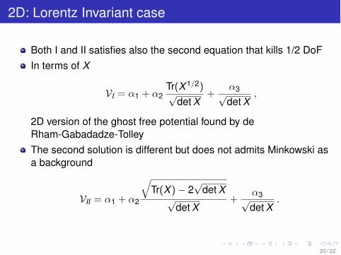
Both I and II satisfies also the second equation that kills 1/2 DoFIn terms of X
VI = ↵1 + ↵2Tr(X 1/2)p
det X+
↵3pdet X
,
2D version of the ghost free potential found by deRham-Gabadadze-TolleyThe second solution is different but does not admits Minkowski asa background
VII = ↵1 + ↵2
qTr(X )� 2
pdet X
pdet X
+↵3pdet X
.
20 / 22

university-logo
2D: Lorentz Invariant case
Both I and II satisfies also the second equation that kills 1/2 DoFIn terms of X
VI = ↵1 + ↵2Tr(X 1/2)p
det X+
↵3pdet X
,
2D version of the ghost free potential found by deRham-Gabadadze-TolleyThe second solution is different but does not admits Minkowski asa background
VII = ↵1 + ↵2
qTr(X )� 2
pdet X
pdet X
+↵3pdet X
.
20 / 22

university-logo
2D: Loentz Breaking Case
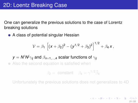
One can generalize the previous solutions to the case of Lorentzbreaking solutions
A class of potential singular Hessian
V = �1
h(x + �2)
2 � (y1/2 + �3)2i1/2
+ �4 x ,
y = NiNj�ij and �n=1,...,4 scalar functions of �ij
Also the second equation is satisfied when
�2 = constant �4 = �1/2�4
Unfortunately the previous solutions does not generalizes to 4D
21 / 22
university-logo
2D: Loentz Breaking Case
One can generalize the previous solutions to the case of Lorentzbreaking solutions
A class of potential singular Hessian
V = �1
h(x + �2)
2 � (y1/2 + �3)2i1/2
+ �4 x ,
y = NiNj�ij and �n=1,...,4 scalar functions of �ij
Also the second equation is satisfied when
�2 = constant �4 = �1/2�4
Unfortunately the previous solutions does not generalizes to 4D
21 / 22

university-logo
Conclusions
Deforming GR is very difficultA randomly picked deforming potential propagates 5+1 DOF;one is a ghost around Minkowski spaceThe condition for having 5 DoF can can be encoded in a setdifferential equationsIn 2D, for the the Lorentz invariant case the solutions is uniqueThere is no known underlying symmetry to get the very specialform of V required for having 5 DoFV is likely to be destabilized by matter’s quantum correctionsPhenomenology (original motivation) is difficult
22 / 22


![Neutrino pathways to cosmology - ffp14.cpt.univ-mrs.frffp14.cpt.univ-mrs.fr/DOCUMENTS/SLIDES/VALLE_Jose_W.F.pdf · RENO: 800 days [talk by Seon-Hee Seo@ICHEP2014] Daya Bay: 621 days](https://img.pdfslide.net/doc/110x75/6009857d021d252e1a074234/neutrino-pathways-to-cosmology-ffp14cptuniv-mrs-reno-800-days-talk-by-seon-hee.jpg)


![Constructive Identities for Physicsffp14.cpt.univ-mrs.fr/DOCUMENTS/SLIDES/RODIN_Andrei.pdf · topos theory to higher topos theory viz. homotopy type theory [viz. Univalent Foundations]](https://img.pdfslide.net/doc/110x75/5edc799fad6a402d666725b9/constructive-identities-for-topos-theory-to-higher-topos-theory-viz-homotopy-type.jpg)