Embed Size (px)
Citation preview

Title: A web scraping framework for stock price modelling using deep learning methods. Author: Aleix Fibla Salgado Advisor: Salvador Torra Porras Department: Econometrics, Statistics and Spanish Economy Academic year: 2018/2019
Degree in Statistics

i
Declaration of Authorship
I, Aleix FIBLA SALGADO, declare that this thesis titled, “A web scraping frameworkfor stock price modelling using deep learning methods.” and the work presented init are my own. I confirm that:
• This work was done wholly or mainly while in candidature for a research de-gree at this University.
• Where any part of this thesis has previously been submitted for a degree orany other qualification at this University or any other institution, this has beenclearly stated.
• Where I have consulted the published work of others, this is always clearlyattributed.
• Where I have quoted from the work of others, the source is always given. Withthe exception of such quotations, this thesis is entirely my own work.
• I have acknowledged all main sources of help.
• Where the thesis is based on work done by myself jointly with others, I havemade clear exactly what was done by others and what I have contributed my-self.
Signed:
Date: 28/06/2019

ii
Abstract
Aleix FIBLA SALGADO
A web scraping framework for stock price modelling using deeplearning methods.
This work aims to shed light to the process of web scraping, emphasizing its im-portance in the new ’Big Data’ era with an illustrative application of such methodsin financial markets. The work essentially focuses on different scraping methodolo-gies that can be used to obtain large quantities of heterogenous data in real time.Automatization of data extraction systems is one of the main objectives pursued inthis work, immediately followed by the development of a framework for predic-tive modelling. applying neural networks and deep learning methods to the dataobtained through web scraping. The goal pursued is to provide the reader withsome remarkable notes on how these models work while allowing room for furtherresearch and improvements on the models presented.
Key words: Big data, neural networks, deep learning, web scraping, stock pricemodelling, time series.
AMS classification: 82C32 - Neural Nets.

iii
Acknowledgements
Foremost, I should like to express my sincere gratitude to my advisor, Dr. SalvadorTorra Porras. This work would not have been possible unless his continuous sup-port, patience, motivation and tremendous knowledge in the field of neural net-works and financial markets.
Besides my advisor, I also owe my deepest gratitude to Dra. Manuela AlcañizZanón, who encouraged me for initiating my studies in Statistics, and guided methrough my entire academic career to become a statistician with her invaluable ad-vice.
Last but not least, I express my deepest appreciation to Pau Casas Bonet andSilvia Sardà Rovira for assisting me with their expertise and insightful suggestionsin financial matters.
iv
Contents
Declaration of Authorship i
Abstract ii
Acknowledgements iii
1 The Big Data era 11.1 Introduction to Big Data . . . . . . . . . . . . . . . . . . . . . . . . . . . 11.2 A new programming paradigm . . . . . . . . . . . . . . . . . . . . . . . 3
1.2.1 How do machines learn? . . . . . . . . . . . . . . . . . . . . . . . 41.2.2 Machine Learning tasks . . . . . . . . . . . . . . . . . . . . . . . 51.2.3 Training Data and test data . . . . . . . . . . . . . . . . . . . . . 61.2.4 Assessing the outcome of learning . . . . . . . . . . . . . . . . . 71.2.5 A primer in Deep Learning . . . . . . . . . . . . . . . . . . . . . 8
1.3 Machine Learning in Finance . . . . . . . . . . . . . . . . . . . . . . . . 9
2 Web scraping Tools in Finance 112.1 The Net as a data source . . . . . . . . . . . . . . . . . . . . . . . . . . . 112.2 Net interactions and networked programs . . . . . . . . . . . . . . . . . 132.3 Overview of alternative data . . . . . . . . . . . . . . . . . . . . . . . . . 14
3 Data Acquisition 163.1 Web Data Extraction . . . . . . . . . . . . . . . . . . . . . . . . . . . . . 16
3.1.1 Geting data from yahoo finance . . . . . . . . . . . . . . . . . . . 203.1.2 Geting news data from reuters . . . . . . . . . . . . . . . . . . . 22
3.2 Variables . . . . . . . . . . . . . . . . . . . . . . . . . . . . . . . . . . . . 263.3 Exploratory Data Analysis . . . . . . . . . . . . . . . . . . . . . . . . . . 27
3.3.1 Company pricing data . . . . . . . . . . . . . . . . . . . . . . . . 273.3.2 News data . . . . . . . . . . . . . . . . . . . . . . . . . . . . . . . 35
4 Methods 404.1 Theoretical considerations . . . . . . . . . . . . . . . . . . . . . . . . . . 41
4.1.1 Universal approximation theorem . . . . . . . . . . . . . . . . . 414.1.2 Activation functions . . . . . . . . . . . . . . . . . . . . . . . . . 424.1.3 Optimization . . . . . . . . . . . . . . . . . . . . . . . . . . . . . 44
4.2 VADER Sentiment analysis . . . . . . . . . . . . . . . . . . . . . . . . . 464.3 LSTM for time series prediction . . . . . . . . . . . . . . . . . . . . . . . 50
5 Results 545.1 Unidimensional LSTM prediction . . . . . . . . . . . . . . . . . . . . . . 555.2 Multidimensional LSTM prediction . . . . . . . . . . . . . . . . . . . . . 59
6 Concluding remarks 64

v
A Python class objects 66A.1 Reuters news crawler . . . . . . . . . . . . . . . . . . . . . . . . . . . . . 66A.2 LSTM data processor . . . . . . . . . . . . . . . . . . . . . . . . . . . . . 69A.3 LSTM model definition . . . . . . . . . . . . . . . . . . . . . . . . . . . . 71
B Natural Language Processing 74B.1 Stop Words . . . . . . . . . . . . . . . . . . . . . . . . . . . . . . . . . . . 74B.2 Punctuation List . . . . . . . . . . . . . . . . . . . . . . . . . . . . . . . . 84B.3 Negate List . . . . . . . . . . . . . . . . . . . . . . . . . . . . . . . . . . . 84B.4 Booster Dictionary . . . . . . . . . . . . . . . . . . . . . . . . . . . . . . 85B.5 Special case idioms . . . . . . . . . . . . . . . . . . . . . . . . . . . . . . 87
Bibliography 88

vi
List of Figures
3.1 Example of DOM . . . . . . . . . . . . . . . . . . . . . . . . . . . . . . . 183.2 Evolution of Adjusted Close Prices . . . . . . . . . . . . . . . . . . . . . 283.3 Volume traded (in hundreds of millions) . . . . . . . . . . . . . . . . . . 293.4 Distribution of stock returns . . . . . . . . . . . . . . . . . . . . . . . . . 303.5 Distribution of stock returns in 2018 . . . . . . . . . . . . . . . . . . . . 333.6 SMA, 2012/01/01 - 2019/06/10 . . . . . . . . . . . . . . . . . . . . . . . 343.7 Stock returns cluster map . . . . . . . . . . . . . . . . . . . . . . . . . . 353.8 Adj close price cluster map . . . . . . . . . . . . . . . . . . . . . . . . . 363.9 Candlestick chart MSFT . . . . . . . . . . . . . . . . . . . . . . . . . . . 373.10 Candlestick chart JNJ . . . . . . . . . . . . . . . . . . . . . . . . . . . . . 373.11 Candlestick chart JPM . . . . . . . . . . . . . . . . . . . . . . . . . . . . 383.12 Top words in headlines . . . . . . . . . . . . . . . . . . . . . . . . . . . . 393.13 Top words in news . . . . . . . . . . . . . . . . . . . . . . . . . . . . . . 39
4.1 Correlation between headlines and normal news sentiment scores . . . 494.2 An unrolled RNN . . . . . . . . . . . . . . . . . . . . . . . . . . . . . . . 514.3 LSTM architecture diagram . . . . . . . . . . . . . . . . . . . . . . . . . 52
5.1 Unidimensional point-by-point prediction . . . . . . . . . . . . . . . . . 565.2 Unidimensional multi-sequence prediction . . . . . . . . . . . . . . . . 585.3 Multidimensional multi-sequence prediction (compound) . . . . . . . 605.4 Multidimensional multi-sequence prediction ( volume) . . . . . . . . . 615.5 Multi-sequence prediction on complete stock data . . . . . . . . . . . . 625.6 Full-sequence prediction on complete stock data . . . . . . . . . . . . . 63

vii
List of Tables
3.1 Stock data: Variables . . . . . . . . . . . . . . . . . . . . . . . . . . . . . 263.2 Highest stock returns . . . . . . . . . . . . . . . . . . . . . . . . . . . . . 313.3 Lowest stock returns . . . . . . . . . . . . . . . . . . . . . . . . . . . . . 313.4 News from the day before abnormal returns . . . . . . . . . . . . . . . 313.5 Stock returns standard deviation . . . . . . . . . . . . . . . . . . . . . . 323.6 Stock returns standard deviation in 2018 . . . . . . . . . . . . . . . . . . 323.7 Number of news retrieved from Reuters . . . . . . . . . . . . . . . . . . 363.8 Average wordcount of headlines and news . . . . . . . . . . . . . . . . 37

viii
List of Abbreviations
ACM Association for Computing MachineryAI Artificial IntelligenceAPI Application Programming InterfaceBDA Big Data AnalyticsCSS Cascading Style SheetsDNA Deoxyribonucleic acidDOM Document Object ModelEDA Exploratory Data AnalysisGDP Gross Domestic ProductHTML HyperText Markup LanguageHTTP HyperText Transport ProtocolICA Independent Component AnalysisIT Information technologyLOOCV Leave-one-out cross validationLSTM Long-short term memoryNLP Natural Language ProcessingNN Neural Network, typically an Artificial Neural NetworkPCA Principal Component AnalysisSMA Simple Moving AveragesSVM Support Vector MachinesTCP/IP Transmission Control Protocol / Internet ProtocolVADER Valence Aware Dictionary and sEntiment ReasonerW3C World Wide Web Consortium
1
Chapter 1
The Big Data era
1.1 Introduction to Big Data
The last decade has seen the birth of what some call ’the industrial revolution ofdata’. With advent of Web 2.0, the amount of published information and data col-lected is raising exponentially, up to the point that experts believe 90% of today’sdata has been generated in merely the last two years 1. The aforementioned revo-lution encompasses, not only increments in the amount of data generated but alsoprominent advances in other drivers of the data process such as the pace at whichdata is coming in or the diversification of data sources.
The term ’Big Data’ was first used in an ACM paper by Michael Cox and DavidEllsworth in 1997 (Cox and Ellsworth, 1997). Despite this first reference, it was JohnMashey, a year after, the one credited for coming up with the term Big data, endow-ing it with its modern meaning. These first voices noticed enormous incrementsin the amount of data that was generated year after year. By that time, the Big Dataphenomenon was perceived as an incredible boost in the quantity and availability ofpotentially rellevant data, sometimes referred to as an ‘information explosion’. Mr.Cox and Mr. Ellsworth defined the term ’big data’ as follows: “Visualization pro-vides an interesting challenge for computer systems: data sets are generally quitelarge, taxing the capacities of main memory, local disk, and even remote disk. Wecall this the problem of big data. When data sets do not fit in main memory (in core),or when they do not fit even on local disk, the most common solution is to acquiremore resources.” A noticeable remark from their terminology is that big data wasinitially perceived as a challenge, in the form of a misalignment between data gen-eration and data processing capabilities available by that time. Experts in the fieldalike (Denning, 1990; Lesk, 1997; Crane, 1997) were highly concerned about the realnecessity of finding new ways of both data storage and processing, seeing a wholeuniverse of opportunities in front of their eyes. The combination of this growing tor-rent of data and further advances in computing systems such as cloud computing,Handoop or the rise of machine learning have largely contributed to the launch ofthe big data era.
Unfortunately, there is still huge controversy about the precise definition of BigData, as it is a broad concept, related to many disciplines and encompassing differ-ent types of data. However, even though lacking a formal definition, it goes withoutsaying that, in the last few years, Big Data has become a buzz word. The term gainedpopularity roughly across every field of study, creating applied disciplines of a widevariety of subjects. In general, the term Big Data is used to refer to any collection ofdata so massive and complex that exceeds the processing capabilities of traditionaldata management systems and techniques. Regarding the purposes of this paper,
1 source IBM: Bringing Big Data to the enterprise.
Chapter 1. The Big Data era 2
(Jothimani, Shankar, and Yadav, 2018) provide an accurate description of what BigData is. Authors argue that the term refers to large data being generated continu-ously in the form of unstructured data produced by heterogeneous groups of ap-plications. The prior definition entitles three prominent characteristics, commonlyused to give meaning to the term Big Data (see Laney, 2001).
Volume, Velocity and Variety, sometimes referred to as the three Vs, are the di-mensions frequently used to characterize Big Data. Volume has probably the moststraightforward connotation as it refers to the massive amount of data generated,collected and stored through records, transactions, files, tables, etc. The total num-ber of bytes of data out there is truly mind-boggling and continually increasing atan accelerated pace 2. Experts have already coined the term ’astronomical scale’ todescribe the size of Big Data and there are numerous challenges related to dealingwith this massive amount of information and the necessity to store it efficiently. Ad-ditional challenges arise in data processing due to volume, as more volume usuallyimplies a higher cost and a worse performance.
Velocity indicates the speed at which data is flowing in or out. Contrary to tra-ditional data collection techniques such as probability-based surveys, what we havenow is a torrent of data flowing in continuously. It is even possible to say that nowa-days data is “harvested” rather than explicitly collected, providing data scientistswith real time data and automatic updates. However, data processing systems donot always match its production rate and opportunities are dismissed as sometimesit is extraordinarily challenging to deal with huge volumes of real time data.
Finally, Variety refers to the increase in the amount and heterogeneity of datasources. The time when only public institutions were responsible for dealing withdata issues has come to an end; today trillions of data are generated from a wide va-riety of applications, devices, sensors, etc. Heterogeneity has usually a direct impacton the complexity of data generated. Even though tabular structured data is stillpredominant and relevant for data scientists, today a much wider variety of datastructures are being used to solve problems. Images, text or geolocations are exam-ples of more unstructured data which has created a world of opportunities but alsomade the analysis more complex to handle.
Recently, new Vs have been introduced to the Big Data community as new chal-lenges and opportunities have been emerging. The first of these late Vs is Veracity.Big Data heterogeneity sometimes implies noisy, biased, uncertain or even volatiledata. Veracity refers to the quality of the data and it is vital to make it operational aslow quality data will inevitably lead to a poor analysis. Capitalizing on big data op-portunities might offer a great advantage in decision making but, at the same time,data based decisions will be valuabluable only if data, the raw material of the wholeprocess, is of a satisfactory quality and consistent over time. Reliability of the datasource, accuracy, consistency of formats or relevance are aspects that definetely haveto be taken into consideration when working with Big Data.
Together with Veracity, another V has recently come to the Big Data scenario andthis one is Valence. Alike Valence in chemistry, a higher Valence means greater dataconnectivity. It measures the ratio of directly or indirectly connected data items thatcould occur within the connectivity potential of the collection. Holding this defini-tion, it is clear that the Valence of a collection of data is dynamic and, apparently,it will increase over time enriching the information embeeded and capturing data
2 In the sixth edition of DOMO’s report it is estimated that by 2020, every person on earth willgenerate 1.7MB of data per second.
Chapter 1. The Big Data era 3
from other networks. In a hypothetical universe of data, Valence might be seen asdensities that measure the extent to which data is concentrated.
Nevertheless, what is at the heart of the Big Data challenge, is the capacity ofturning all the previous Vs into truly useful business value. Conversations aroundBig Data take place everywhere whilst organizations keep on exploring new ways toeffectively deploy these big volumes aiming to capture value for their stakeholders.The previously mentioned ’astronomical scale’ has made experts skeptical about theprevalent imperative of always finding new appraches to deal with Volume. Thefocus now is shifting from size to value as for some ’big’ is no longer the definingparameter, but rather how ’valuable’ the data is. Accordingly, the term ’Smart Data’has come into play referring to feasible volumes that provide a reasonable numberof insights.
In light of the above, it is possible to argue that Big Data has contributed to therise of a data-driven era, where BDA are used in every sector and its possibilitiesappear to be endless. The growing of available data is a trend recognized world-wide and value is arising from this new resource. In fact, the list of opportunitiesthat Big Data presents knows no boundaries. It can uncover hidden behavioural pat-terns and shed light on people’s interests and intentions, in a way that makes evenpossible to anticipate events. Everyday, we all unconciously leave behind our digi-tal footprints and this data can yield extremely useful information. In the scientificsphere, BDA revealed the genetic origin of diseases, which ultimately led to person-alized patient care, proved neutrinos have non-zero masses3 and even increased theunderstanding of our galaxy, bringing light to topics such as dark matter and darkenergy. Regarding potential challenges or risks surrounding BDA, someone couldthink about how much data to store, how much this will cost, whether the data willbe secure or how long it must be maintained (Michael and Miller, 2013). In addition,Big Data also presents new ethical challenges involving the preservation of privacylikewise needed to be adressed.
Overall, Big Data is changing our lifes in both small and large ways. It delvesdeep into our understanding of fundamental issues and has already shifted our fo-cus to experimenting rather than formulating hypothesis. Some may argue Big Datais even changing the scientific method as we have more data available and, conse-quently, testing becomes cheaper. This idea of experimenting and finding statisticalevidence is closely related with the next section and, although improved powers ofdiscenrment and a better understanding of the real opportunities and risks involvingBig Data are still needed, this phenomenon will unquestionably become an essentialpart of our lifes.
1.2 A new programming paradigm
Troughout the last decade, Big Data has become a reality in more and more fields ofresearch. However, it is also well-known that the ratio of data volume increase hassurpassed the increase in processing power. In addition, data-collection technolo-gies are becoming more and more efficient and advances like sensor networks, theInternet of Things, and others, foresee that this volume will continue to increase (Tri-funovic et al., 2015). Today’s major challenge for data scientists is to get real valuefrom such quantities of data and, to achieve this goal, being capable of processingthis huge amount of information is a must. In view of the limitations that traditional
3 This achievement came from the SDSS project, a major multi-spectral imaging and spectroscopicredshift survey using a dedicated 2.5-m wide-angle optical telescope.
Chapter 1. The Big Data era 4
processing units had when facing Big Data problems, added to the necessity of lever-aging these cutting-edge resources, developers opted for shifting the programmingparadigm to a more data oriented approach.
In general, programming consists in creating applications by breaking down re-quirements into composable problems that can be coded against. Before the Big Dataera, developers used to figure out the rules behind the data, then write a code capa-ble of making the calculations to finally output a result. However, with Big Dataproblems it is many times more reasonable to focus on the data rather than on theprocess, as both the bulk of data and its nature makes impossible to even think aboutany process behind it. This new paradigm consists in getting lots of examples of bothinputs and outputs and use the machine to infer the rules between the data and theanswers. Contrary to traditional programming, where rules and data were the in-puts to the machine, Machine Learning rearranges this diagram by putting data andanswers into the machine to get the rules out. Broadly speaking, Machine learning isall about feeding the machine with lots and lots of examples so that, regardless of therelationship behind the data and the answers, the computer is capable of learningsuch patterns and distinguish things. Its mathematical analogous would be findinga formula that maps X to Y.
1.2.1 How do machines learn?
Machine Learning originated in an enivornment where, although not at the samepace, the availability of data and computing power were rapidly evolving. Thesetwo drivers, fostered the development of new statistical methods and disciplines fordealing with large datasets as much of the information is valuable, only if there wasa systematic way of making sense from it all.
Arthur Samuel, a pioneer in the study of artificial intelligence in 1950s and 1960s,said that machine learning is "the design and study of software artifacts that givescomputers the ability to learn without being explicitly programmed". This initialgrasp of what "learning" really meant to computers stressed the fact that, to bealigned with the volume of data flowing in, computers should learn from experienceeither with or without human supervision. A few years later, Tom M. Mitchell, asoftware engineer from Carnegie Mellon University, purposed a more formal defin-tion: " A program can be said to learn from experience E with respect to some classof tasks T and performance measure P, if its performance at tasks in T, as measuredby P, improves with experience E. Mitchell’s rationale was based on the fact thatlearning must ultimately lead to better actions. Accordingly, computers can only besaid to learn if they are capable of using experience to improve their performance onsimilar experiences in the future.
This conception of learning is remarkably similar to the human learning process.It starts with some data input (observation, recall, feel, memory storage etc.) fol-lowed by an abstraction process to translate the data into broader representationsand finally generalize this abstraction to form a basis of action (Lantz, 2015). No-tice these steps do follow the scientific method, with the difference that the machineknow is responsible for the abstraction process which, in other words, implies for-mulating an hypothesis using events observed as the benchmark. The last stageinvolves testing the previously forged hypothesis to determine if it is stable andconsistent enough to be generalized.
Likewise, The fundamental goal of machine learning relies on inducing unknownrules from examples of the rule’s application to finally transform data into intelligentactions. In machine learning, data is no longer a set of Xs to be fitted in some model,
Chapter 1. The Big Data era 5
but instead, it has to be treated in a more abstract way focusing on the informationencoded in it. Furthermore, to built efficient algorithms it is also important to makean intelligent use of all the information present in the data and try to maximize itsuse because Big Data rapidly turns problems infeasible. As an example, think abouta university exam in which the professor provides students with a set of ten thou-sand questions and tells them the exam will be fifty of them. Instead of memorizingten thousand answers, it appears more reasonable to study a bunch of questions, geta general notion of the topics covered and then use this knowledge in the exam.
1.2.2 Machine Learning tasks
In line with the idea of learning presented in previous section, machine learningtasks and methods can be decomposed in two major types; supervised and unsu-pervised learning. They both profess the idea of utilizing experience to improvefuture performance but, at the same time, can be thought of as occupying oppositeends of the machine learning spectrum.
On the one hand, supervised learning is based on predicting an outcome using aground truth as input or, in other words, having prior knowledge of the output val-ues for the sample data. Supervised learning is usually adopted for problems wherethe program learns from a pair of labeled inputs and outputs, namely examples withthe right answers. On the other hand, unsupervised learning aims to learn the inher-ent structure of the data without using explicitly labeled inputs. Since the groundtruth is missing, it is sometimes difficult to assess the model’s performance in un-supervised learning. However, these last machine learning systems might be hihglyuseful in exploratory analysis, as they automatically identify structures in the data,and for dimensionality reduction. Some types of problems require semi-supervisedlearning methods, a collection of data and techniques located on the spectrum be-tween supervised and unsupervised learning 4.
By and large, the vast majority of supervised learning algorithms perform ei-ther classification or regression tasks. In both cases, the objective is to find struc-tures or specific relationships in the input data that make possible to attain correctoutput results. Classification problems consist on predicting discrete values (labels,classes, categories) for one or more explanatory variables. On the contrary, in regres-sion problems the programm predicts a continuous value for the response variable.Examples of algorithms employed in supervised learning are SVM, Naive Bayes,Logistic Regression, Artificial Neural Networks and Random Forests, also namedDecision Trees.
In the other side of the coin, clustering and dimensionality reduction are two ofthe most common tasks performed in unsupervised learning problems. Clusteringassigns observation to different groups or clusters based on a similarity measure ina way that observations within a cluster are similar to each other but different fromthe ones in other groups. It is an extremely useful technique for exploring a dataset.Dimensionality reduction is another common unsupervised learning problem usedwhen the number of explanatory variables is too large to work with. This method isbased on detecting the explanatory variables that account for the greatest variabil-ity in the response and, consequently, remove from the analysis the ones capturingnoise as their relevance will be lower. Among the most popular algorithms in unsu-pervised learning, we might encounter the wide range of clustering algorithms (seeAggarwal, 2014), PCA or ICA.
4See Zhu and Goldberg, 2009 for more information on semi-supervised learning techniques.
Chapter 1. The Big Data era 6
Depending on the user needs and the characteristics of the data available, oneor other of these analysis is more advisable. In the case of labeled data, both super-vised and unsupervised learning are plausible alternatives, whereas the last one isthe only possible option in the abscence of labels. Furthermore, supervised learningis generally used in predictive analytics while unsupervised learning can be em-ployed in earlier stages of the data process for exploratory purposes like clustering,density estimation or representation learning. The majority of methods employed inthis paper fall under the umbrella of supervised learning as "right answers" will bealways available.
1.2.3 Training Data and test data
The collection of examples that comprise the learning experience in supervised learn-ing is called the training set. Similarly, the set of examples used to assess the per-formance of the trained model is called the test set. Broadly speaking, the generalprocedure in machine learning is to fit the model on the training set, learn about datarelationships and finally make predictions on data that was not trained. It seems rea-sonable not to include any training data in the test set because it will be difficult toevaluate whether the algorithm has learned to generalize from the training set or hassimply memorized the outputs. The purpose of machine learning is to generalize re-lationships from the training dataset and infer them when dealing with new exam-ples. A program that memorizes "too well" the training data by learning an overlycomplex model will output accurate predictions for the training set, but probablyfail to predict response values for new examples. Memorizing the training set ex-cessively accurately but not succeding in test data predictions is called over-fitting,a problem that will be discussed in later sections.
Without regard to the algorithm used, traning and test datasets are the two basicelements needed in Machine Learning and depending on th nature and structure ofthe data, both can be obtained in different ways. Most of the time, data is collectedand stored in a single unit containing all the observations 5 and the classic approachis to split this data into training and test datasets.
Theory does not provide specific requirements for the sizes of the partitions andthey may vary depending on the data available and the speed at which the algorithmis capable of learning the underlying data structure. Indeed, there are a lot of factorsinfluencing the previously mentioned speed rate like the algorithm’s performance,the heterogeneity of the information or the amount of noise in the training dataset.As an example, think about an algorithm trained on a large collection of noisy, biasedand sometimes incorrectly labeled data. Even with extra computing power and along learning process, it is very likely the algorithm will not perform better thananother one trained on a smaller but more representative dataset.
Some experts argue a third set of observations, called a validation or hold-outset, is sometimes required (Hackeling, 2017). Splitting the dataset into training andtest data has its dangers. Although not a big concern in Big Data, the partiton has tobe random, in a way both subsets are small representations of the population. Forinstance, in classification problems all labels/classes/states must be present in bothtraining and test data. The opposite will inevitably result in overfitting and crossvalidation is a good option to avoid it, particularly when training is scarce. Cross-validation is a deep topic, there are several methods and applications, also outside
5 each observation consistñs of an observed response variable and a set of observed explanatoryvariables.
Chapter 1. The Big Data era 7
Machine Learning (Arlot and Celisse, 2010). On the whole, the rational behind cross-validation is closely related to bootstrap and resampling principles; estimates yieldfrom different train/test splits should not be statistically significant assuming bothobjects are independent and observations are i.i.d. Therefore, it is a good way ofverifying that the split is, indeed, random.
K-Folds and LOOCV are two popular methods used in cross-validation. Thefirst one divides the training dataset in k partitions (or folds) and the algorithm istrained using all but one of them, which is left for testing purposes. Subsequentiterations rotate partitions so that, in the end, the algorithm is trained and assessedon all the training data. On the other hand, LOOCV treats each observation as onefold and builds the model using averages 6. Leaving LOOCV aside, the number offolds considered represents a tradeoff between bias and variance errors, in additionto higher computational costs when more folds are added.
1.2.4 Assessing the outcome of learning
Recall, any learning process is characterized by turning abstracted knowledge ob-tained from inputs into a form that can be utilized for future action and improveperformance on similar tasks. The term generalization is more than often used torefer to this idea of getting real knowledge out of observational inputs. However, inBig Data problems it is not feasible to examine one-by-one all the potential conceptsbehind the ocean of data flowing in thus, machines employ heuristics to make edu-cated guesses about which are the most important concepts to be taken into consid-eration for further predictions. These heuristics necessarily generate imperfectionsin machine learning tasks, which are noticed when confronting the trained modelwith the validation set. The final step in machine learning problems is to determinethe success of learning in spite of its prediction errors.
Unexplained variations in the data result in prediction errors which mainly fallunder the umbrella of the model’s bias and variance. The first one is associatedwith systematic sources of variability so that the model produces similar but biasedresults for an input regardless of the training set it was trained with. On the contrary,variance is more related to random variations derived from sampling the trainingdata. Ideally, the objective would be to tackle both causes of prediction errors butusually decreasing one implies increasing the other. For this reason, this phenomeonis usually referred to as the bias-variance- trade-off and depending on the context,the optimal balance may vary. Models with high variance are inflexible but errorsare easier to tackle while models with high variability often overfit the training dataand much more difficult to generalize well to new cases. Solutions to overfittingare spefific to different machine learning and most of the time rely upon intrinsiccharacteristics of the algorithm employed (Hawkins, 2004).
Indentifying and understanding errors in prediction outputs is extremely im-portant for model diagnosis and a first step through improvements. In the field ofstatistics, metrics are necessary since any decision should be supported with datafacts and machine learning is not an exception. Metrics are extremely important toquantify the outcome of learning. In supervised learning, many performance mea-sures are based on prediction errors whereas, unsupervised learning problems eval-uate some attributes of the data structures discovered as error signals are missing.Finally, although somehow aligned, most performance measures are only valid for a
6 Notice how computationally expensive is LOOCV; the number of training sets resulting from allthe combinations will equal the number of observations.
Chapter 1. The Big Data era 8
specific machine learning task and each problem should be evaluated using metricsthat represent the costs associated with making errors in the real world.
1.2.5 A primer in Deep Learning
The term Deep Learning, refers to training neural networks, an artificial creation in-spired by human neural networks. A regular NN consists of a bunch of processingunits, usually named neurons, each one producing a sequence of valued activationsof some process. These neurons can be activated with external stimulus or throughconnections with other active neurons, depending on the relative position of the neu-ron to the network and how connections are configured. Of course, this is how ourbrains work and throughout the last decade, the relationship between these neuralnetworks and models used in mathematics and computational sciencies have drawnthe attention of a number experts in both fields.
By definition, Deep Learning is a sub-category of Machine Learning and they areboth ought to fall inside the scope of AI. In its broadest definition, Machine Learninginvolves the design and implementation of algorithms than can learn from data.Deep learning is just one possible way of doing it, preaching the learning throughexamples and unveiling an outperformance in finiding patterns out of raw data.
Neural Networks are the heart of Deep Learning and they are nothing but ap-proximations of functions arranged in multiple layers, which when multiplied bythe input return an output close to the real value. As said before, a Neural Networkis made of neurons, little nodes where the learning takes place. Each neuron takesa data input, computes a function and outputs new data. At the same time, theseneurons are stacked together to compose the different layers.
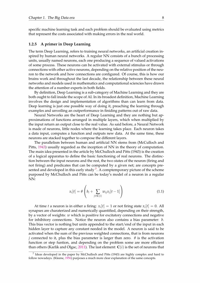
The parallelism between human and artificial NN stems from (McCulloch andPitts, 1943) usually regarded as the inception of NN in the theory of computation.The main idea presented in the article by McChulloch and Pitts (1943) is the creationof a logical apparatus to define the basic functioning of real neurons. The distinc-tion between the input neurons and the rest, the two states of the neuron (firing andnot firing) and predicates that can be computed by a given net; are concepts pre-sented and developed in this early study 7. A comptemporary picture of the schemepurposed by McChulloch and Pitts can be today’s model of a neuron in a regularNN:
xi[t] = q
0
@bi + Âj2C(i)
wijxj[t � 1]
1
A (1.1)
At time t a neuron is in either a firing: xi[t] = 1 or not firing state xi[t] = 0. Allsynapses are charaterized and numerically quantified, depending on their strength,by a vector of weights: w which is positive for excitatory connections and negativefor inhibitory connections. Notice the neuron also contains a bias parameter: b.This bias vector is nothing but units appended to the start/end of the input in eachhidden layer to capture any constant needed in the model. A neuron is said to beactivated when the sum of the previous weighted connections, that is from neuronsj connected to it, plus the bias parameter is larger than zero. q is the activationfunction or step funtion, and depending on the problem some are more efficientthan others (Karlik and Olgac, 2011). The last element: C(i) is the set of neurons that
7 Ideas developed in the paper by McChulloch and Pitts (1943) are highly complex and hard tofollow nowadays. (Kleene, 1956) purposes a much more clear explanation of the same concepts.
Chapter 1. The Big Data era 9
impige on neuron i. Accordingly, the state of neuron i will be determined trough theweighted addition of values from previous neurons in C.
Arranging multiple processing layers with different activations allows compu-tational models to learn representations of data with multiple levels of abstraction.Starting with the raw data, each layer transforms previous level representation intoa new one at a higher, more abstract level. With enough transormations, very com-plex data patterns can be learned and irrelevant information is discriminated at eachlevel. A deep-learning architecture is a multilayer stack of different modules, all (ormost) of them subject to learning and many of which compute non-linear input-output mappings (LeCun, Bengio, and Hinton, 2015). These mappings are drivenby a loss function that measures the error between the hypothetical layer outputscores when compared to the real values. Each layer adjusts the weights by meansof a gradient vector which indicates the marginal increment or decrement in the lossfunction if the weights were increased by a small amount. Finally, before moving onto the next layer, the weights are modified in the opposite direction to the gradientvector and this output will be the input to the new module. Repeating this proce-dure a number of times allows the machine to obtain a very precise X-Y mappingwhich can be applied to new input data and continue with the learning process.
The major success of Deep Learning is that layers of features are not designedby humans, contrary to classical inference. Machines are empowered with total free-dom to determine the optimal mapping from whatever function of data and weightsusing a general-purpose learning procedure. The field is making major advances insolving previously unfeasible problems with enormous contributions in many do-mains. Image and speech recognition might be the most popular applications ofDeep Learning techniques but do not forget, predictive modelling in DNA codingand gene expression, particle acceleration or natural language understanding usingmethods such as sentiment analysis or topic classification (LeCun, Bengio, and Hin-ton, 2015).
In the near future, Deep Learning is expected to have even a greater successbecause it requires very little human intervention and due to its high flexibility andmachine oriented approach it can be applied to almost any discipline and can takeadvantage of the tremendous increase in the amount of data available in this new BigData era. New architectures and algorithms are continually being developed andmachines have proven to become better year after year at prediction tasks thanks toDeep Learning, a fact that will undoubtedly accelearate its expansion.
1.3 Machine Learning in Finance
Economic and financial prediction models are of great relevance and general interest.Just imagine the possibilities that might offer being able to anticipate an increasein the price of a commodity, foresee GDP growth rate for next semester or predictfuture returns from a company’s shares. Having read previous sections, someonemight think that Machine Learning is the key to succeed in all these predictive tasksbut, wihout being false, the financial world is sometimes quite daunting. Economictheory is more than often unclear about the variables that influence a certain outputand it suggests that many of them are spread throughout different types of datafor instance economic, social or political. Dealing with such disparate data sourcesis not easy and if reasearchers pursue to capture all factors that might impact somefinancial magnitude, the collection of potentially relevant data will probably becometoo large to handle. In addition, the way these sources interact is extremely complex,
Chapter 1. The Big Data era 10
presumably non-linear functions, which are not properly specified by the theory. Asa consequence, a number of predictive models in finance are build via trial and errorwith little theoretical justification and sometimes accuracy is adversely affected.
In the world of finance, artificial intelligence could be helpful in a lot of differentareas and the value of machine learning is becoming more apparent by the day. Overthe past few years, the big players in the industry have witnessed profound changeswith the entry of new joiners adopting quantitative investment methods to competein the marketplace. The so-called Fintech companies have experienced great successin brining financial services to a new level where machine learning plays a key role.In response, big firms had to adopt an AI approach in some of their services, becauseif not they would have been left behind in not many years. The flow of informationin financial markets is now quicker than ever and machine learning seems to be thekey for investors to chase these fleeting opportunities and keep up with a highlysensitive environment.
The applications of machine in the financial sector are huge and diverse. Bothregression and classification methods are extremely useful in areas such as fraudprevention, risk management, investment prediction, customer service, loan under-writing, document interpretation or algorithmic trading; among others. This pa-per focuses on the uses and functionalities that big data and machine learning canbring to stock prediction with emphasis on its advantages against traditional analy-sis methods.
Stock prices are ought to be very volatile, dynamic and susceptible to quickchanges as they are supposedly influenced by multiple factors both within the finan-cial domain of companies and outside the scope of financial markets. With properinformation about stock prices with a suitable level of accuracy, the overall loss oninvestments might be reduced and the whole society can benefit from it through abetter allocation of resources, avoiding wastes and promoting a healthy expansionof financial markets where people can invest more confidently. Transparency is de-finetely an issue in investment for all the stakeholders involved in the process andmachine learning provides a framework where truthful informed financial decisionsare about to be a reality. However, as said before, lots of unknown factors surroundstock prices and the expertise from professional trades is hard to replace. In addi-tion, famous theorems like the efficient market hypothesis or the random walk hy-pothesis come to say that future stock prices are completely unpredictable and theydo not depend on past data, henceforth there are not patterns to be exploited sincetrends do not exist (Shah, 2007). Machine learning and Deep Learning methods arenow challenging these theorems and it might be still early but investors willing toadapt these state-of-the-art technologies will likely have an edge in the new financialsector.
Following sections introduce a stock price forecasting framework where NN areused to predict future stock movements and alternative data is also feeded into themodel in an attempt to capture potentially relevant unknown factors and enhancethe accuracy of the model, ultimately seeking to avoid blind investment behaviours.Webscraping methods are used in data acquisition stages since their vision is per-fectly aligned with the Big Data train of thought posed in this chapter. Next sectionpresents a detailed outline of webscraping techniques together with the reason whyautomatizing data acquisition and even pre-processing is necessary to exploit all theopportunies that stem from Big Data.
11
Chapter 2
Web scraping Tools in Finance
2.1 The Net as a data source
It is a well-known fact that the World Wide Web is immense and growing at an ex-traordinary fast pace every second. Its exact size, however, is difficult to determineas it is hard for a counter to tackle small IT sites and a large portion of the Web, pop-ularly known as the Deep Web, is hidden and not easy to access. Without forgettingthe above considerations what we can say is that, in terms of weight, the World WideWeb is measured in zettabytes (1 zettabyte = 1021 bytes) and so forth, such a gigan-tic universe of data presents a major opportunity to turn it into valuable insights.The scope and potential of the abundance of data in the network sounds excitingbut it can be both blessing and curse. As probably the biggest source of informationavailable in the world, the World Wide Web is an optimal illustration of the Big Dataframework discussed in previous chapter. Lots of relevant information, as hiddentreasures in a vast sea of data; along with variety, velocity and veracity issues.
The data growth rate on the internet is soaring every year and, as a consequence,data comes predominantly in an unstructured form (Chaulagain et al., 2017). Sincethis data is not prepared neither to be fitted in any model nor to be analyzed in anyway, information churning might become a problem. Furthermore, the data on theweb is a constant state of flux; it is continously updated and modified. Therefore,web-based data collection techniques must be fast and flexible enough to keep pacewith this constant change. Ultimately, due to the voluntary and often anonymousnature of user interactions with the Web, added to the lack of a body responsible forassessing the quality and availability of the data, some of this information is alwayssurounded with uncertainity. In light of the above, and with the irruption of BigData technologies, it is becoming more and more crucial for both researchers andpractitioners to find efficient ways of exploring the network and retrieving relevantinformation. Harnessing such volumes of heterogenous data from the web often re-quires a highly customizable programmatic approach (Krotov and Tennyson, 2018a)although, for those not familiar with programming languages, todays’ web is be-coming overwhelmed with handy resources that most of the time will do the workfor you.
Data acquisition is the starting point of any data science project and the inputscan be obtained from either private sources like company’s internal data or pub-lic sources, and it is here where a world of possibilities opens up. Public sourcescomprise official data from government institutions, journals or, more generally, anydata that can be found on the web regardless of whether it is open data or you haveto purchase it. All the data employed in this paper falls under the umbrella of opendata and it is obtained from the net through webscraping. At odds with what mostpeople think, open data not only refers to tidy and structured data published on theweb by some entity. The concept is more general and, in fact, it does not conlfict
Chapter 2. Web scraping Tools in Finance 12
with how data is structured, presented or shared. Open data merely refers to thebelief that some data should be freely available to everybody and all players shouldbe able to use and republish it without any copyright restrictions, patents or othermechanisms of control (Berners-Lee, Hendler, and Lassila, 2001). Therefore, no mat-ter how the data looks like or where it comes from, every byte of information free touse, reuse and redistribute is considered open data.
In addition, this paper seeks to exemplify previous arguments regarding theWorld Wide Web and reinforce the idea that the network is vast and messy but,with the proper tools, is possible to extract real value out of this universe of infor-mation. As said before, there are different ways of gathering data from the web;some users may interact with an API, others may use data mining or text miningand the ones lacking programming skills will simply click on the download link of adata provider website. Troughout the last decade, different terms have been coinedto refer to this act of extracting data from websites: web scraping, web harvesting,web crawling or web data extraction; are just a few examples. However, the defini-tion of this terminology is still vague and more than often leads to confusions andcontroversies. As an example, for many authors alike (Krotov and Tennyson, 2018a,Boeing and Waddell, 2017), althought the term typically refers to automated pro-cesses, web scraping is solely the act of extracting data from websites. Accordingly,manually downloading data from a website could be considered web scraping in themost user-friendly level. Others understand web scraping from a standpoint closeto parsing text files formatted in HTML and XPath (Krotov and Tennyson, 2018b).In theory, web scraping is the practice of gathering data through any means otherthan a program interacting with an API or a human using a browser. A text min-ing approach does not seem wrongheaded as the previous interpretation is typicallyacomplished by a program that queries a web server, requests data (usually html)and parses the code obtained to extract the useful information. However, recentstudies (Lawson, 2015) put the emphasis on the web exploration step arguing thatthe real added value that webscraping offers is the possibility of gathering and pro-cessing large amounts of data rather than viewing one page at a time which is whata browser can attain. Therefore, with convenient scrapers, one can access databasesspanning thousands of webpages at once. Again, this can be attained through dif-ferent methods and one more time text mining is an option since changing dates ina web link is usually enough to access historical data. In the absence of consensusregarding the boundaries of webscraping and in line with the purposes of this work,any retrieval of information from the web entailing some sort of automatization to-gether with an organized approach will be considered webscraping.
Likewise analysis where the data is obtained in the form of a table from an officialdata provider website or by quering a database, here the source is the net itself andthe goal pursued is to find efficient ways of exploring it, downloading the desiredinformation and clean it so the final output from this intial data acquisition step isa tidy dataset ready for futher modelling. This objective is achieved through web-scraping and in this respect, it involves not only retrieving the data from the webbut also, when required, turn unstructured data into a tidy and properly arrangeddataset. Finally, as said before, the whole process should be fully automatized andreproducible capturing updates and outputting real time results.
Chapter 2. Web scraping Tools in Finance 13
2.2 Net interactions and networked programs
Contrary to what most people think, the World Wide Web and the Internet are notsynonyms. The first, refers to a descentralized interconnection of different devicesby means of a set of protocols known as TCP/IP protocols, while the World WideWeb is a system that manages the information shared over the Internet through theso-called HyperText Transport Protocol or HTTP. This network protocol is actuallyquite simple and there are multiple built-in supports in almost all progamming lan-guages that make it relatively easy to create network connections and retrieve dataover them. These modules are like files, except that they provide a two-way con-nection between the network and the device in which they are executed. Therefore,both sides can read and write to the same program and the protocol sets the rulesthat regulate this user network interaction 1.
In today’s world, almost every person in developed countries navigates the net-work everyday but, for the vast majority, its mechanisms still seem quite mysterious.Computer interfaces have progressed to the point where the net can be extremelyvaluable for users even though they do not have any idea about how it works. In-ternet browsers are the main responsibles of this and, although it is not necessaryto understand what the network is doing in all our interactions to succeed at web-scraping, web data extraction techniques usually require to connect to the newtorkat a lower level. In fact, the exchange of information between a user and the networktakes place without the intervention of a browser. Broadly speaking, the Internet isonly the mean to request some action from a web server and the browser is merelycode that interprets the server response and gets the user back the same data in moreattractive formats such as images, videos, music, formatted text etc 2. As said before,capabilities of web browsers are also present in almost all programming languagesand the value that own-built webscrapers can bring to the analysis is the opportunityto interepret server responses in the most convenient way.
The main output of the previously mentioned request/response mechanism reg-ulated by the HTTP protocol is an hypertext document, commonly known as a web-page. HTML is the predominant language for encoding web architectures and it islargely supported by W3C consortium. HTML pages can be thought of a form ofsemi-structured data following a nested structure where information is stored andaccessed using tags. Each HTML element is associated with a speficic tag, repre-sented with angled brackets, and typically coming in pairs for both opening andclosing the element. These tags can be be also thought as element insertions in awebpage they can be progitably used in the design of suitable scrapers. The listof elements in a webpage and their corresponding tags is lengthy, including hy-perlinks, images, paragraphs or videos, among others. However, although most ofthe webpage content is found in the HTML code, it is also important to acknowl-edge that webpages might also include other items such as CSS or Javascript objects.These extra features are not particularly relevant for the purposes of this paper butdefinetely a factor to be taken into cosnideration from a programmatic perspectivesince languages are different and they can be misleading.
1 See a description of the HyperText Transport Protocol in the following document: HypertextTransfer Protocol – HTTP/1.1
2 Internet browsers are relatively new compared to the Internet, first ones were released in thenineties, and, as any other piece of code, they can be re-written, re-used or re-formated (Lawson,2015).
Chapter 2. Web scraping Tools in Finance 14
Literature provides a number of different strategies and techniques adopted inthe field of Web Data Extraction (Ferrara et al., 2014) and most of the time human ex-pertise is required to define the rules of the data extraction process. The challenge isto stablish a high degree of automatization to reduce human efforts as much as pos-sible and this often goes hand in hand with having a good knowledge of the domain.(Krotov and Tennyson, 2018b) purpose a general three-step process to characterizeweb-data extraction strategies:
• The initial phase involves examining the website architecture using a web in-spector to understand how the data is stored at a technical level. The objectiveis to get a general idea of how the information is encoded, likely HTML lan-guage, and feed the scraper with these inputs. Ideally, the underlying structureof the website captured by the scraper should be extrapolated to others of sim-ilar nature.
• Second phase concerns running a previously developed piece of code that au-tomatically browses the web and retrieves the desired information. The under-standing of the domain comes to play in this stage as it will guide the scraperto fetch the needed data.
• Finally, there is also a "Data Organization" step which involves cleaning thedata retrieved, sometimes coming in an unstructured form, and arrange it in adataset. This last stage makes the data ready for further analysis.
Even though the previous sequence is coherent, the three stages are often inter-twined. Many times, the programer will have to go back and forward until the finaltidy dataset is obtained since the process might have to be applied, for instance, tosmaller data units like rows or individual chuncks of information retrieved fromdifferent websites. One more time, the common note along all stages is human su-pervision, particularly when analyzing the website architecture. It is probably themost tedious part and where more innefficiencies are concentrated since some do-mains often require to be examined individually.
Over the last decade, various strategies have been developed in the field of webscraping to deal with previously mentioned concerns and reduce the commitment ofhuman domain experts. A possible way forward involves the adoption of MachineLearning algorithms capable of identifying the structure of webpages and extractingthe useful information. Some of these systems are discussed in further research sec-tions but the basic outline consists of training a program with numerous examples ofweb architectures so that after the tranining it becomes competent in autonomouslyextracting data from similar, or even different, domains.
2.3 Overview of alternative data
In general, and particularly in whe world of finance, the idea of bringing to the stageall the Big Data culture is to empower businesses with new insights and foster thedevelopment of data driven models for decision making to ultimately create value.Recent advances in web data extraction techniques enable a more efficient searchand retrieval of information from different sources and allow traditional datasets tobe enriched with new data. In line with previous discussion about the factors thatmight have an impact on some financial indicator, more than often traditional dataused in finance or economics fail to capture enough inputs to conduct accurate fore-casts 1. One of the contributions of Big Data in this field involves the possibility of
Chapter 2. Web scraping Tools in Finance 15
enriching traditional datasets like production rates, historical financial results fromfirms or GDP series with other types of data that will hopefully seize external vari-ables that might impact a certain output but have not been contemplated before. Theinformational advantage provided by these new sources of data can be in the formof uncovering new relevant information not included in traditional datasets, or an-ticipating it before traditional sources do. This new information is popularly knownas alternative data and, although veracity issues are not the major concern as manytimes the model itself will deploy innacurate information, the three Vs are more thanvalid to characterize these new sources. The term alternative data is chiefly used infinance with little visibility in other fields of research and it refers to all the infor-mation gathered from non-traditional data sources which can provide new insightsbeyond those which traditional data is capable of providing.
The concreteness of what does alternative data include varies from industry toindustry. In finance, the market of alternative data is quite fragmented but recently,JP Morgan developed a framework to classify alternative data into three main cate-gories based on the manner in which data was generated:
• Individuals: Information collected at an individual level that will provide in-sights about market trends, consumer behaviour, public opinion, etc.
• Business Processes: Data from agents in the market with a new higher level ofdetail.
• Sensors: This category includes data from satellites or geolocations.
More often than not, it is not easy to evaluate the relevance that a specific type ofalternative data might have on a financial magnitude. In addition, there is little stan-darization for most alternative data offerings whereby most of the time the data willcome in an ustructured or semi-structured form. Accordingly, pre-processing is usu-ally a must before getting this data ready and compatible with traditional datasets.For this reason, webscraping is usually the mean to gather alternative data since aprogrammatic approach and an automatized pre-processing is required to make thewhole process feasible.
There are lots of success stories related to the use of alternative data sourcesto improve financial processes, specially in predictive modelling matters. A fewexamples are the use of consumer transaction data to trade individual stocks, twittersentiment data to trade the broad equity market or geolocation data to estimate realactivity in some area. In this paper, the power of alternative data is put to test usingsentiment data from news’ headlines to make stock price predictions more accurate.The idea is that news data will provide the model with insights about market trendsand expectations so that the program will learn how to anticipate future changesand outscore stock markets in reaction time.
16
Chapter 3
Data Acquisition
First step in any data science project involves the acquisition and pre-processing ofthe data required for further analysis and modelling. In line with the idea devel-oped in previous sections, the underlying principle behind the obtention of the datais strongly based on webscraping, attempting to reduce human efforts as much aspossible, and offering a user-friendly approach with a higher degree of automati-zation. These procedures will most likely be reproducible with a ’manually’ dataobtention process but, and this is one of the main justifications for using webscrap-ing, in a context as dynamic as financial markets, velocity of data is a sucess factorand the optimization of processes is essential. Furthermore, when deciding whichdata to use in a project its cost is an important consideration. As said before, all thedata employed is open data hence there are not any direct costs associated with itspurchase. Nevertheless, the oppotunity cost of time invested in acquiring and ana-lyzing the data is also relevant and webscraping pursues to generate savings here.
The Big Data universe is changing the foundations of the entire data science pro-cess and state-of-the-art methods are a valid patch when resources are scarce or sim-ply when the researcher does not have any theoretical input behind the phenomenonstudied. Today’s world requires more flexible, adaptative and faster methods to dealwith problems that most of the time demand a prompt response and theoretical con-siderations are limited. Machine Learning, deep learning and all these new analysistools might be the most widely recognized exponent of old methods in data sciencebeing replaced with modern techniques. However, not only the analysis step hassuffered changes, innovations in data acquisition or preprocessing are also remark-able, largely due to webscraping. In the not too distant future, data storage will bea serious concern for computer manufacturers and the current trend is in the direc-tion of web resources and interconnected servers, trying to minimize the amount ofinformation locally stored. Therefore, in data extraction, a webscraper, designed ad-hoc for a specific problem, seems to be the most efficient way to obtain the desiredinformation while optimizing the capacity of memory resources.
3.1 Web Data Extraction
The majority of approaches to extracting data from the Web are designed ad-hocto operate on a specific domain 1. Accordingly and, although most of the time pro-gramming languages provide users with built-in modules that ease the work, certainprogramming skills and a good knowledge of html language and data structres aredesirable to built efficient scrapers.
1 (Ferrara et al., 2014) discusses the potential of cross-fertilization methods and the possibility of re-using Web Data Extraction techniques originally developed in a given application to multiple domains.
Chapter 3. Data Acquisition 17
Programming languages like Python or R have utilities called sockets which arenothing more than regular files with the peculiarity that they provide a two-wayconnection between two programs thus the user can both read and write to thesame socket. These sockets use the HTTP protocol to emulate a browser and makenetwork connections and data retrieval very easy to handle.
1 import socket2
3 mysock = socket . socket ( socket . AF_INET , socket .SOCK_STREAM)4 mysock . connect ( ( ’ data . pr4e . org ’ , 80) )5 cmd = ’GET http :// data . pr4e . org HTTP/1.0\ r\n\r\n ’ . encode ( )6 mysock . send (cmd)7
8 while True :9 data = mysock . recv ( 1 0 2 4 )
10 i f ( len ( data ) < 1) :11 break12 p r i n t ( data . decode ( ) )13
14 mysock . c l o s e ( )
LISTING (3.1) A simple socket
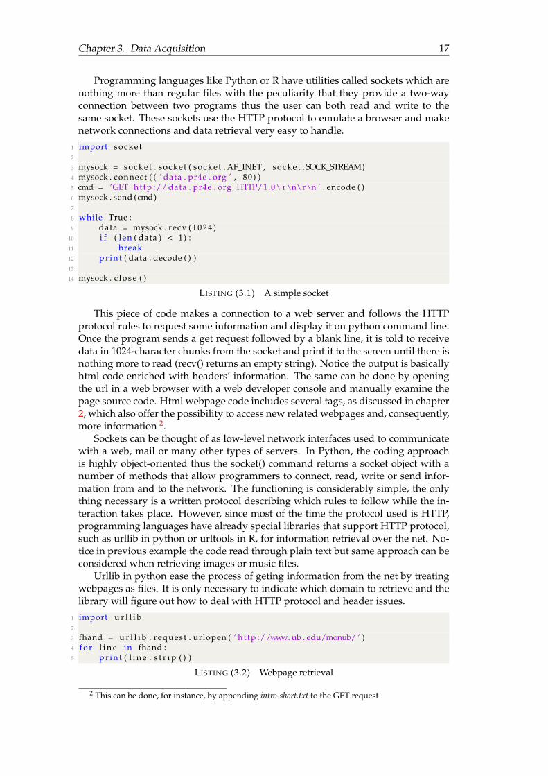
This piece of code makes a connection to a web server and follows the HTTPprotocol rules to request some information and display it on python command line.Once the program sends a get request followed by a blank line, it is told to receivedata in 1024-character chunks from the socket and print it to the screen until there isnothing more to read (recv() returns an empty string). Notice the output is basicallyhtml code enriched with headers’ information. The same can be done by openingthe url in a web browser with a web developer console and manually examine thepage source code. Html webpage code includes several tags, as discussed in chapter2, which also offer the possibility to access new related webpages and, consequently,more information 2.
Sockets can be thought of as low-level network interfaces used to communicatewith a web, mail or many other types of servers. In Python, the coding approachis highly object-oriented thus the socket() command returns a socket object with anumber of methods that allow programmers to connect, read, write or send infor-mation from and to the network. The functioning is considerably simple, the onlything necessary is a written protocol describing which rules to follow while the in-teraction takes place. However, since most of the time the protocol used is HTTP,programming languages have already special libraries that support HTTP protocol,such as urllib in python or urltools in R, for information retrieval over the net. No-tice in previous example the code read through plain text but same approach can beconsidered when retrieving images or music files.
Urllib in python ease the process of geting information from the net by treatingwebpages as files. It is only necessary to indicate which domain to retrieve and thelibrary will figure out how to deal with HTTP protocol and header issues.
1 import u r l l i b2
3 fhand = u r l l i b . request . urlopen ( ’ ht tp ://www. ub . edu/monub/ ’ )4 f o r l i n e in fhand :5 p r i n t ( l i n e . s t r i p ( ) )
LISTING (3.2) Webpage retrieval
2 This can be done, for instance, by appending intro-short.txt to the GET request
Chapter 3. Data Acquisition 18
The output object is the html contents of the webpage and it can be treated assort of a text file (although still byte literal) and, accordingly, read through it using afor loop. This level of interaction is higher than using a socket as the information isready to be deployed and, up to this point, it is even possible to perform simple taskssuch as word counts or tackle specific tags that might provide the desired informa-tion. As an example, differences aside, the google search engine works at this levelof abstraction; it looks at the source code of one webpage, extract links to other re-lated pages, retrieve them, and finally use its famous page rank algorithm to displaythe most relevant finds in response to a user search. Web spiders use this principleto navigate the web, as it quite straightforward since links within a webpage aredefined with an ’a’ tag in html thus not even complicated regular expressions areneeded to find them 3.
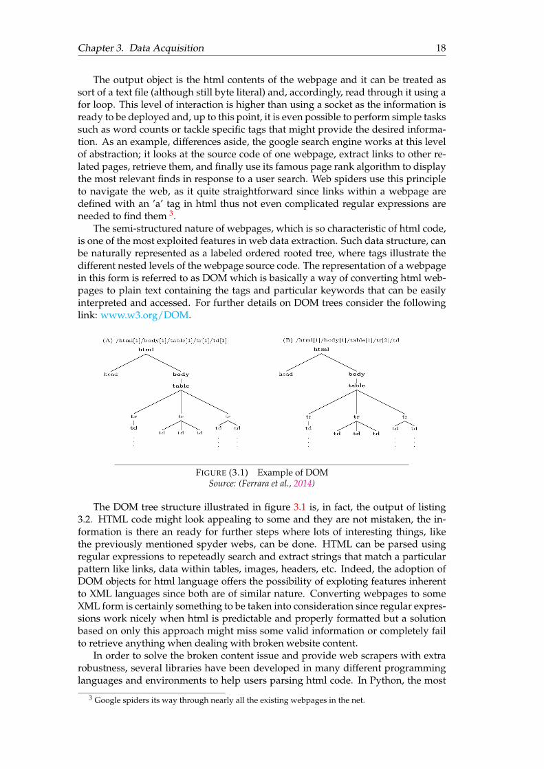
The semi-structured nature of webpages, which is so characteristic of html code,is one of the most exploited features in web data extraction. Such data structure, canbe naturally represented as a labeled ordered rooted tree, where tags illustrate thedifferent nested levels of the webpage source code. The representation of a webpagein this form is referred to as DOM which is basically a way of converting html web-pages to plain text containing the tags and particular keywords that can be easilyinterpreted and accessed. For further details on DOM trees consider the followinglink: www.w3.org/DOM.
FIGURE (3.1) Example of DOMSource: (Ferrara et al., 2014)
The DOM tree structure illustrated in figure 3.1 is, in fact, the output of listing3.2. HTML code might look appealing to some and they are not mistaken, the in-formation is there an ready for further steps where lots of interesting things, likethe previously mentioned spyder webs, can be done. HTML can be parsed usingregular expressions to repeteadly search and extract strings that match a particularpattern like links, data within tables, images, headers, etc. Indeed, the adoption ofDOM objects for html language offers the possibility of exploting features inherentto XML languages since both are of similar nature. Converting webpages to someXML form is certainly something to be taken into consideration since regular expres-sions work nicely when html is predictable and properly formatted but a solutionbased on only this approach might miss some valid information or completely failto retrieve anything when dealing with broken website content.
In order to solve the broken content issue and provide web scrapers with extrarobustness, several libraries have been developed in many different programminglanguages and environments to help users parsing html code. In Python, the most
3 Google spiders its way through nearly all the existing webpages in the net.
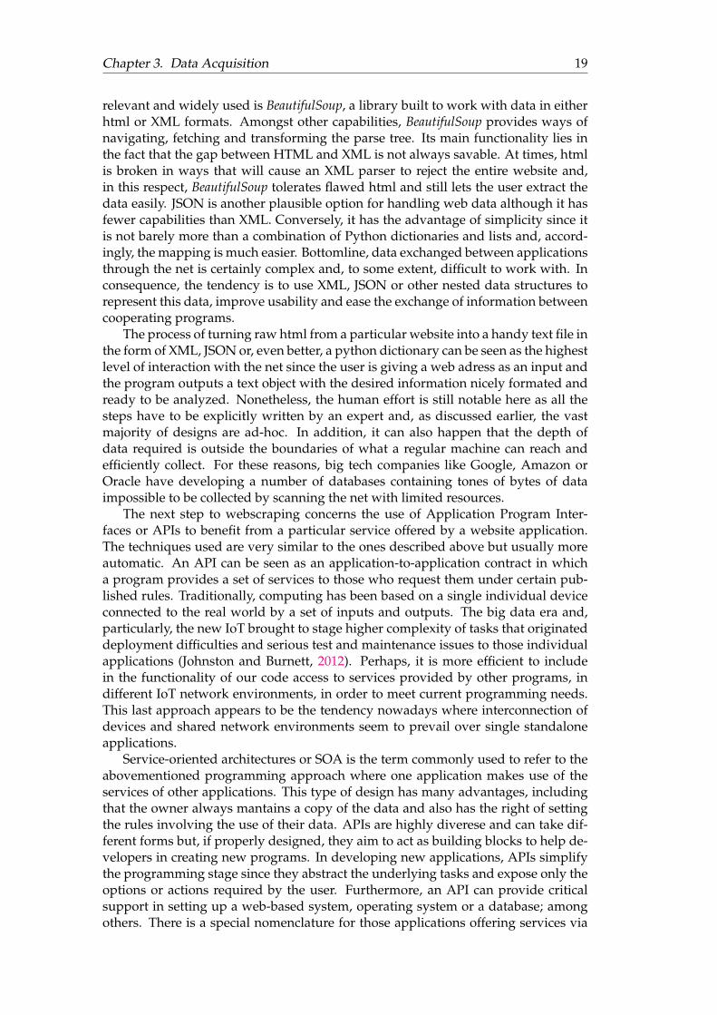
Chapter 3. Data Acquisition 19
relevant and widely used is BeautifulSoup, a library built to work with data in eitherhtml or XML formats. Amongst other capabilities, BeautifulSoup provides ways ofnavigating, fetching and transforming the parse tree. Its main functionality lies inthe fact that the gap between HTML and XML is not always savable. At times, htmlis broken in ways that will cause an XML parser to reject the entire website and,in this respect, BeautifulSoup tolerates flawed html and still lets the user extract thedata easily. JSON is another plausible option for handling web data although it hasfewer capabilities than XML. Conversely, it has the advantage of simplicity since itis not barely more than a combination of Python dictionaries and lists and, accord-ingly, the mapping is much easier. Bottomline, data exchanged between applicationsthrough the net is certainly complex and, to some extent, difficult to work with. Inconsequence, the tendency is to use XML, JSON or other nested data structures torepresent this data, improve usability and ease the exchange of information betweencooperating programs.
The process of turning raw html from a particular website into a handy text file inthe form of XML, JSON or, even better, a python dictionary can be seen as the highestlevel of interaction with the net since the user is giving a web adress as an input andthe program outputs a text object with the desired information nicely formated andready to be analyzed. Nonetheless, the human effort is still notable here as all thesteps have to be explicitly written by an expert and, as discussed earlier, the vastmajority of designs are ad-hoc. In addition, it can also happen that the depth ofdata required is outside the boundaries of what a regular machine can reach andefficiently collect. For these reasons, big tech companies like Google, Amazon orOracle have developing a number of databases containing tones of bytes of dataimpossible to be collected by scanning the net with limited resources.
The next step to webscraping concerns the use of Application Program Inter-faces or APIs to benefit from a particular service offered by a website application.The techniques used are very similar to the ones described above but usually moreautomatic. An API can be seen as an application-to-application contract in whicha program provides a set of services to those who request them under certain pub-lished rules. Traditionally, computing has been based on a single individual deviceconnected to the real world by a set of inputs and outputs. The big data era and,particularly, the new IoT brought to stage higher complexity of tasks that originateddeployment difficulties and serious test and maintenance issues to those individualapplications (Johnston and Burnett, 2012). Perhaps, it is more efficient to includein the functionality of our code access to services provided by other programs, indifferent IoT network environments, in order to meet current programming needs.This last approach appears to be the tendency nowadays where interconnection ofdevices and shared network environments seem to prevail over single standaloneapplications.
Service-oriented architectures or SOA is the term commonly used to refer to theabovementioned programming approach where one application makes use of theservices of other applications. This type of design has many advantages, includingthat the owner always mantains a copy of the data and also has the right of settingthe rules involving the use of their data. APIs are highly diverese and can take dif-ferent forms but, if properly designed, they aim to act as building blocks to help de-velopers in creating new programs. In developing new applications, APIs simplifythe programming stage since they abstract the underlying tasks and expose only theoptions or actions required by the user. Furthermore, an API can provide criticalsupport in setting up a web-based system, operating system or a database; amongothers. There is a special nomenclature for those applications offering services via
Chapter 3. Data Acquisition 20
their APIs over the web, they are popularly known as web services.Data acquisition by means of one or many APIs is probably the highest level of
interaction with the network since most of underlying implementations, which wereclearly visible and explicitly programmed in the socket case, are no longer neededto be set but, instead, driven by the same API. All the previous net interactions, withtheir respective abstraction levels, ought to fall within the sphere of webscrapingalthough, as seen, the way the code is written is totally different.
Subsequent sections and subsections present the two types of data used in fur-ther models. In both cases, the major bulk of work is conducted by different APIs de-spite basic knowledge about network interaction and html language will be neededat some point. The core data for the experiment is mainly stock data retrieved fromyahoo finance by means of the pandas-datareader, a Python library that offers upto date remote data access for pandas, another open source library (BSD licensed)used for handling data structures and basic analysis in Python. If familiar withpandas data structures, the pandas-datareader is an optimal option since it extractsdata from different Internet domains such as Google Finance, Enigma, Morningstar,Eurostat or the World Bank 4via their respective APIs, and turns it into a pandasdataframe. Similarly, a news scraper is designed to get data from Reuters, an inter-national news agency with a web portal very suitable for scraping purposes.
The abovementioned data sets are the raw materials needed in the analysis goingon in this paper. The first and core, a collection of financial data from stock listedfirms. Second, an assortment of news that will enrich the information provided byfinancial markets. Complementarily, webscraping offers a systematic approach tothe obtention of data and object-oriented programming, so characteristic of Python,will be present in both scenarios.
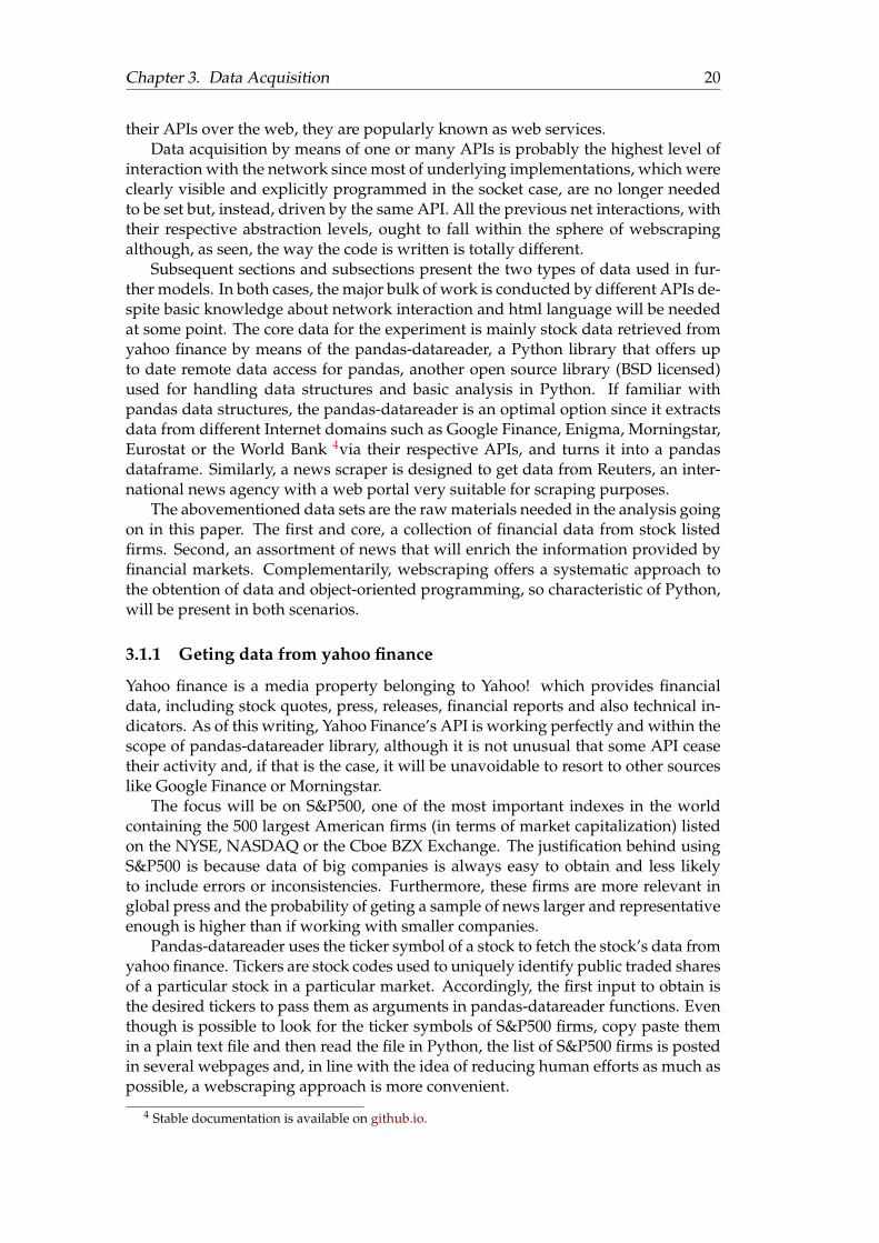
3.1.1 Geting data from yahoo finance
Yahoo finance is a media property belonging to Yahoo! which provides financialdata, including stock quotes, press, releases, financial reports and also technical in-dicators. As of this writing, Yahoo Finance’s API is working perfectly and within thescope of pandas-datareader library, although it is not unusual that some API ceasetheir activity and, if that is the case, it will be unavoidable to resort to other sourceslike Google Finance or Morningstar.
The focus will be on S&P500, one of the most important indexes in the worldcontaining the 500 largest American firms (in terms of market capitalization) listedon the NYSE, NASDAQ or the Cboe BZX Exchange. The justification behind usingS&P500 is because data of big companies is always easy to obtain and less likelyto include errors or inconsistencies. Furthermore, these firms are more relevant inglobal press and the probability of geting a sample of news larger and representativeenough is higher than if working with smaller companies.
Pandas-datareader uses the ticker symbol of a stock to fetch the stock’s data fromyahoo finance. Tickers are stock codes used to uniquely identify public traded sharesof a particular stock in a particular market. Accordingly, the first input to obtain isthe desired tickers to pass them as arguments in pandas-datareader functions. Eventhough is possible to look for the ticker symbols of S&P500 firms, copy paste themin a plain text file and then read the file in Python, the list of S&P500 firms is postedin several webpages and, in line with the idea of reducing human efforts as much aspossible, a webscraping approach is more convenient.
4 Stable documentation is available on github.io.
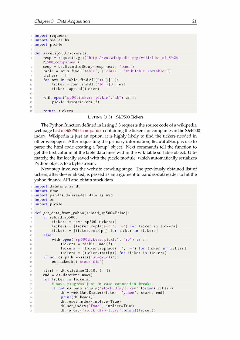
Chapter 3. Data Acquisition 21
1 import reques ts2 import bs4 as bs3 import p i c k l e4
5 def s a ve _ s p 5 0 0 _ t i c k e r s ( ) :6 resp = reques t s . get ( ’ ht tp :// en . wikipedia . org/wiki/ L i s t _ o f _ S%26
P_500_companies ’ )7 soup = bs . Beauti fulSoup ( resp . t e x t , ’ lxml ’ )8 t a b l e = soup . f ind ( ’ t a b l e ’ , { ’ c l a s s ’ : ’ w i k i t a b l e s o r t a b l e ’ } )9 t i c k e r s = [ ]
10 f o r row in t a b l e . f i n d A l l ( ’ t r ’ ) [ 1 : ] :11 t i c k e r = row . f i n d A l l ( ’ td ’ ) [ 0 ] . t e x t12 t i c k e r s . append ( t i c k e r )13
14 with open ( " s p 5 0 0 t i c k e r s . p i c k l e " , "wb" ) as f :15 p i c k l e .dump( t i c k e r s , f )16
17 re turn t i c k e r s
LISTING (3.3) S&P500 Tickers
The Python function defined in listing 3.3 requests the source code of a wikipediawebpage List of S&P500 companies containing the tickers for companies in the S&P500index. Wikipedia is just an option, it is highly likely to find the tickers needed inother webpages. After requesting the primary information, BeautifulSoup is use toparse the html code creating a "soup" object. Next commands tell the function toget the first column of the table data lines within the wikitable sortable object. Ulti-mately, the list locally saved with the pickle module, which automatically serializesPython objects to a byte stream.
Next step involves the website crawling stage. The previously obtained list oftickers, after de-serialized, is passed as an argument to pandas-datareader to hit theyahoo finance API and obtain stock data.
1 import datetime as dt2 import time3 import pandas_datareader . data as web4 import os5 import p i c k l e6
7 def get_data_from_yahoo ( reload_sp500=Fa lse ) :8 i f reload_sp500 :9 t i c k e r s = s a v e _ s p 5 00 _ t i c k e r s ( )
10 t i c k e r s = [ t i c k e r . r e p l a c e ( ’ . ’ , ’� ’ ) f o r t i c k e r in t i c k e r s ]11 t i c k e r s = [ t i c k e r . r s t r i p ( ) f o r t i c k e r in t i c k e r s ]12 e l s e :13 with open ( " s p 5 0 0 t i c k e r s . p i c k l e " , " rb " ) as f :14 t i c k e r s = p i c k l e . load ( f )15 t i c k e r s = [ t i c k e r . r e p l a c e ( ’ . ’ , ’� ’ ) f o r t i c k e r in t i c k e r s ]16 t i c k e r s = [ t i c k e r . r s t r i p ( ) f o r t i c k e r in t i c k e r s ]17 i f not os . path . e x i s t s ( ’ s tock_dfs ’ ) :18 os . makedirs ( ’ s tock_dfs ’ )19
20 s t a r t = dt . datetime ( 2 0 1 0 , 1 , 1 )21 end = dt . datetime . now ( )22 f o r t i c k e r in t i c k e r s :23 # save progress j u s t in case connect ion breaks24 i f not os . path . e x i s t s ( ’ s tock_dfs / { } . csv ’ . format ( t i c k e r ) ) :25 df = web . DataReader ( t i c k e r , ’ yahoo ’ , s t a r t , end )26 p r i n t ( df . head ( ) )27 df . r e s e t _ i n d e x ( i n p l a c e=True )28 df . se t_ index ( " Date " , i n p l a c e=True )29 df . to_csv ( ’ s tock_dfs / { } . csv ’ . format ( t i c k e r ) )
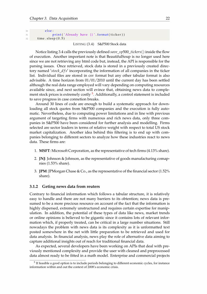
Chapter 3. Data Acquisition 22
30 e l s e :31 p r i n t ( ’ Already have { } ’ . format ( t i c k e r ) )32 time . s leep ( 0 . 5 )
LISTING (3.4) S&P500 Stock data
Notice listing 3.4 calls the previously defined save_sp500_tickers() inside the flowof execution. Another important note is that BeautifulSoup is no longer used heresince we are not retrieving any html code but, instead, the API is responsible for theparsing issues. Once retrieved, stock data is stored in a previously created direc-tory named 0stock_d f s0 incorporating the information of all companies in the tickerlist. Individual files are stored in csv format but any other tabular format is alsoadvisable. A time horizon from 01/01/2010 until the current day has been settledalthough the real data range employed will vary depending on computing resourcesavailable since, and next section will evince that, obtaining news data to comple-ment stock prices is extremely costly 5. Additionally, a control statement is includedto save progress in case connetion breaks.
Around 30 lines of code are enough to build a systematic approach for down-loading all stock quotes from S&P500 companies and the execution is fully auto-matic. Nevertheless, due to computing power limitations and in line with previousargument of targeting firms with numerous and rich news data, only three com-panies in S&P500 have been considered for further analysis and modelling. Firmsselected are sector leaders in terms of relative weight with respect to total US stockmarket capitalization. Another idea behind this filtering is to end up with com-panies belonging to different sectors to analyze how these industries react to newsdata. These firms are:
1. MSFT: Microsoft Corporation, as the representative of tech firms (4.13% share).
2. JNJ: Johnson & Johnson, as the representative of goods manufacturing comap-nies (1.53% share).
3. JPM: JPMorgan Chase & Co., as the representative of the financial sector (1.52%share).
3.1.2 Geting news data from reuters
Contrary to financial information which follows a tabular structure, it is relativelyeasy to handle and there are not many barriers to its obtention; news data is pre-sumed to be a more precious resource on account of the fact that the information ishighly dispersed, extremely unstructured and requires certain expertise for manip-ulation. In addition, the potential of these types of data like news, market trendsor online opinions is believed to be gigantic since it contains lots of relevant infor-mation which, if properly treated, can be critical in a large number situations. Stillnowadays the problem with news data is its complexity as it is unformatted textposted somewhere in the net with little preparation to be retrieved and used fordata analysis. In financial analysis, news play the role of alternative data aiming tocapture additional insights out of reach for traditional financial data.
As expected, several developers have been working on APIs that deal with pre-viously mentioned complexity and provide the user with cleaned and preprocesseddata almost ready to be fitted in a math model. Enterprise and commercial projects
5 If feasible a good option is to include periods belonging to different economic cycles, for instanceinformation within and out the context of 2008’s economic crisis.
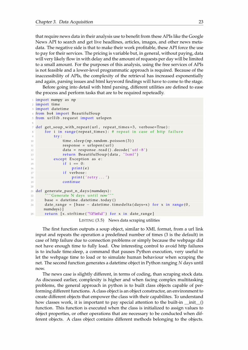
Chapter 3. Data Acquisition 23
that require news data in their analysis use to benefit from these APIs like the GoogleNews API to search and get live headlines, articles, images, and other news meta-data. The negative side is that to make their work profitable, these API force the useto pay for their services. The pricing is variable but, in general, without paying, datawill very likely flow in with delay and the amount of requests per day will be limitedto a small amount. For the purposes of this analysis, using the free services of APIsis not feasible and a lower-level programmatic approach is required. Because of theinaccessibility of APIs, the complexity of the retrieval has increased exponentiallyand again, parsing issues and html keyword findings will have to come to the stage.
Before going into detail with html parsing, different utilities are defined to easethe process and perform tasks that are to be required repeteadly.
1 import numpy as np2 import time3 import datetime4 from bs4 import Beauti fulSoup5 from u r l l i b . request import urlopen6
7 def get_soup_with_repeat ( url , repeat_t imes =3 , verbose=True ) :8 f o r i in range ( repeat_t imes ) : # repeat in case of ht tp f a i l u r e9 t r y :
10 time . s leep ( np . random . poisson ( 3 ) )11 response = urlopen ( u r l )12 data = response . read ( ) . decode ( ’ utf�8 ’ )13 re turn Beauti fulSoup ( data , " lxml " )14 except Exception as e :15 i f i == 0 :16 p r i n t ( e )17 i f verbose :18 p r i n t ( ’ r e t r y . . . ’ )19 continue20
21 def generate_past_n_days ( numdays ) :22 " " " Generate N days u n t i l now " " "23 base = datetime . datetime . today ( )24 date_range = [ base � datetime . t imedel ta ( days=x ) f o r x in range ( 0 ,
numdays ) ]25 re turn [ x . s t r f t i m e ( "%Y%m%d" ) f o r x in date_range ]
LISTING (3.5) News data scraping utilities
The first function outputs a soup object, similar to XML format, from a url linkinput and repeats the operation a predefined number of times (3 is the default) incase of http failure due to connection problems or simply because the webpage didnot have enough time to fully load. One interesting control to avoid http failuresis to include time.sleep, a command that pauses Python execution, very useful tolet the webpage time to load or to simulate human behaviour when scraping thenet. The second function generates a datetime object in Python ranging N days untilnow.
The news case is slightly different, in terms of coding, than scraping stock data.As discussed earlier, complexity is higher and when facing complex multitaskingproblems, the general approach in python is to built class objects capable of per-forming different functions. A class object is an object constructor, an environment tocreate different objects that empower the class with their capabilites. To understandhow classes work, it is important to pay special attention to the built-in __init__()function. This function is executed when the class is initialized to assign values toobject properties, or other operations that are necessary to be conducted when dif-ferent objects. A class object contains different methods belonging to the objects.
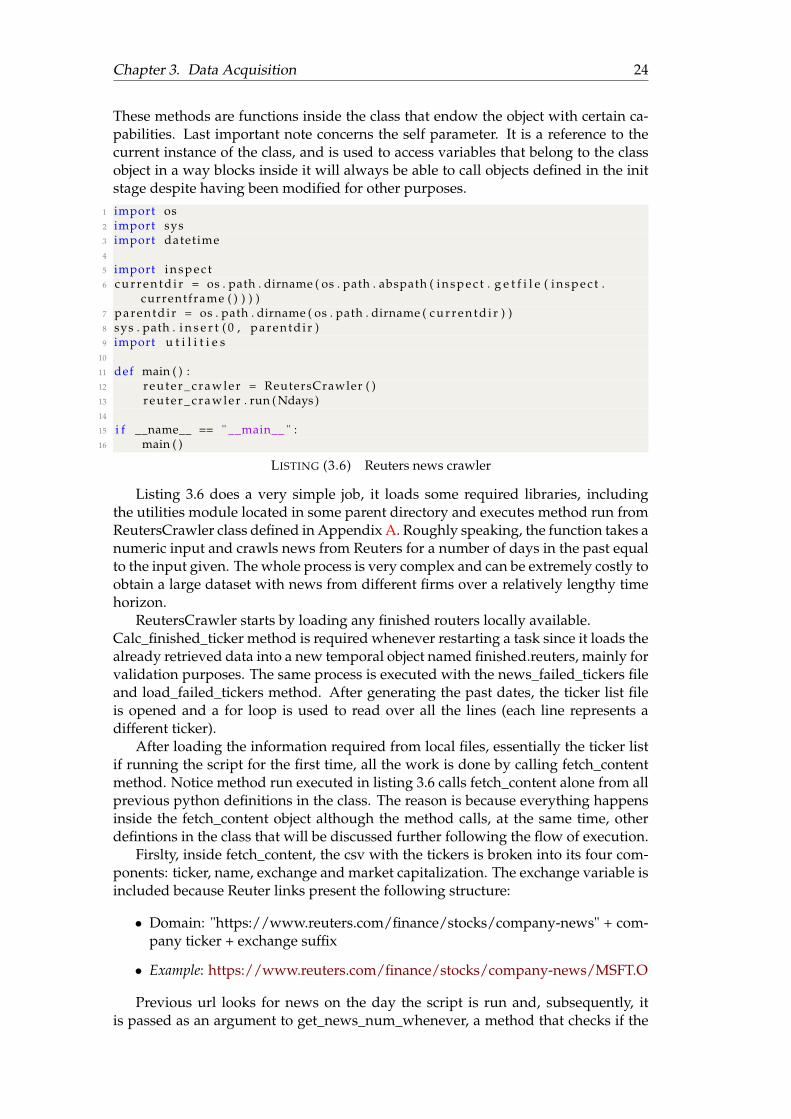
Chapter 3. Data Acquisition 24
These methods are functions inside the class that endow the object with certain ca-pabilities. Last important note concerns the self parameter. It is a reference to thecurrent instance of the class, and is used to access variables that belong to the classobject in a way blocks inside it will always be able to call objects defined in the initstage despite having been modified for other purposes.
1 import os2 import sys3 import datetime4
5 import i n s p e c t6 c u r r e n t d i r = os . path . dirname ( os . path . abspath ( i n s p e c t . g e t f i l e ( i n s p e c t .
currentframe ( ) ) ) )7 parentd i r = os . path . dirname ( os . path . dirname ( c u r r e n t d i r ) )8 sys . path . i n s e r t ( 0 , parentd i r )9 import u t i l i t i e s
10
11 def main ( ) :12 r eu t er _ cr a wl e r = ReutersCrawler ( )13 r eu t er _ cr a wl e r . run ( Ndays )14
15 i f __name__ == " __main__ " :16 main ( )
LISTING (3.6) Reuters news crawler
Listing 3.6 does a very simple job, it loads some required libraries, includingthe utilities module located in some parent directory and executes method run fromReutersCrawler class defined in Appendix A. Roughly speaking, the function takes anumeric input and crawls news from Reuters for a number of days in the past equalto the input given. The whole process is very complex and can be extremely costly toobtain a large dataset with news from different firms over a relatively lengthy timehorizon.
ReutersCrawler starts by loading any finished routers locally available.Calc_finished_ticker method is required whenever restarting a task since it loads thealready retrieved data into a new temporal object named finished.reuters, mainly forvalidation purposes. The same process is executed with the news_failed_tickers fileand load_failed_tickers method. After generating the past dates, the ticker list fileis opened and a for loop is used to read over all the lines (each line represents adifferent ticker).
After loading the information required from local files, essentially the ticker listif running the script for the first time, all the work is done by calling fetch_contentmethod. Notice method run executed in listing 3.6 calls fetch_content alone from allprevious python definitions in the class. The reason is because everything happensinside the fetch_content object although the method calls, at the same time, otherdefintions in the class that will be discussed further following the flow of execution.
Firslty, inside fetch_content, the csv with the tickers is broken into its four com-ponents: ticker, name, exchange and market capitalization. The exchange variable isincluded because Reuter links present the following structure:
• Domain: "https://www.reuters.com/finance/stocks/company-news" + com-pany ticker + exchange suffix
• Example: https://www.reuters.com/finance/stocks/company-news/MSFT.O
Previous url looks for news on the day the script is run and, subsequently, itis passed as an argument to get_news_num_whenever, a method that checks if the
Chapter 3. Data Acquisition 25
ticker has any news and, if true, returns the count. The output is stored in news_numand represents the number of news available on Reuters the day the script is beingrun. However, the goal is to retrieve past news for a given date range, and noticefetch_content method has a date_range argument hence the scraper should be ca-pable of accessing Reuters drop down menu and look for news in the past. Besidesfurther date concerns, up to this point, there are three different paths to follow de-pending on the value of news_num:
• If news_num 6= 0, fetch_within_date_range method is called. This object per-forms 5 tasks:
– Keeps track of the number of days with missing content, initializing thevalue at zero and resetting it every time news are obtained (variable miss-ing_days).
– Controls for whether a retrieved html code has content or not, initializingthe value at False and turning it into True every time news are obtained(variable has_content).
– Loops over the date range and appends "?date=", followed by new_time(date index over date_range), to previous dateless url. This final url takesdates into consideration, the final structure of a Reuters’ link for any pastdate is the following: https://www.reuters.com/finance/stocks/company-news/MSFT.O?date=mmddaaaa
– Retrieves html associated to the previously defined url and stores it as asoup object.
– Calls parse_and_save_news, a method which takes the previous soupobject as input and returns the top story and the new text displayed inReuters.
The corresponding outputs are all automatically converted to csv format andstored in files finished.reuters, news_failed_tickers and news_reuters.
• If the company has news (news_num 6= 0) on the current day, but none ofthem found within the given date range, the ticker is set as LOW priority andsaved in a separate file to be used later, if desired. Variable no_news_daystakes account of the consecutive number of days with no news found and it isrestarted whenver a new is fetched.
• If the company has no news, even with no date range specified, the ticker isadded to the LOWEST priority list.
Overall, all the methotology is oriented towards optimizing the process by firsttargeting webpages in which the program knows in advance that they contain use-ful data. Furthermore, fetch_within_date_range stops the crawler if a company hasno news for a number of consecutive days in the past. The stop crawling limit iscalculated using the number of news found in the current day, thus proportional toan indicator of news frequency. The higher the news count, the longer willigness towait for new data to appear on Reuters. If a forced stop occurs, it is probably dueto some kind of systematic error and the scraper will very rarely find more newsin previous days hence the effort of trying is not worth. Finally, a company mayhave multiple news in a single day but as the information within a day should behighly correlated and, to simplify the process, it is perfectly valid to consider onlytop stories for prediction purposes.
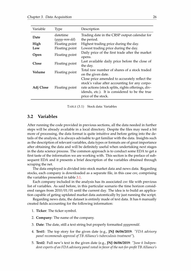
Chapter 3. Data Acquisition 26
Variable Type Description
Date datetime(yyyy-mm-dd)
Trading date in the CRSP output calendar forthe period.
High Floating point Highest trading price during the day.Low Floating point Lowest trading price during the day.
Open Floating point Daily price of the first trade after the marketopens.
Close Floating point Last available daily price before the close ofthe day.
Volume Floating point Total raw number of shares of a stock tradedon the given date.
Adj Close Floating point
Close price amended to accurately reflect thestock’s value after accounting for any corpo-rate actions (stock splits, rights offerings, div-idends, etc.). It is considered to be the trueprice of the stock.
TABLE (3.1) Stock data: Variables
3.2 Variables
After running the code provided in previous sections, all the data needed in furthersteps will be already available in a local directory. Despite the files may need a bitmore of processing, the data format is quite intuitive and before geting into the de-tails of the analysis, it is always advisable to get familiar with the data. Insights suchas the description of relevant variables, data types or formats are of great importanceafter obtaining the data and will be definitely useful when undertaking next stagesin the data science process. The common approach is to conduct some EDA to get afirst taste of the information we are working with. This section is the preface of sub-sequent EDA and it presents a brief description of the variables obtained throughscraping the net.
The data employed is divided into stock market data and news data. Regardingstocks, each company is downloaded as a separate file, in this case csv, comprisingthe variables presented in table 3.1.
Each company included in the analysis has its associated csv file with previouslist of variables. As said before, in this particular scenario the time horizon consid-ered ranges from 2010/01/01 until the current day. The idea is to build an applica-tion capable of geting uptdated market data automtically by just running the script.
Regarding news data, the dataset is entirely made of text data. It has 6 manuallycreated fields accounting for the following information:
1. Ticker: The ticker symbol.
2. Company: The name of the company.
3. Date: The date, still a text string but properly formatted yyyymmdd.
4. Text1: The top story for the given date (e.g., JNJ 06/06/2019: "FDA advisorypanel recommends approval of TB Alliance’s tuberculosis treatment").
5. Text2: Full new’s text in the given date (e.g., JNJ 06/06/2019: "June 6 Indepen-dent experts of an FDA advisory panel voted in favor of the not-for-profit TB Alliance’s
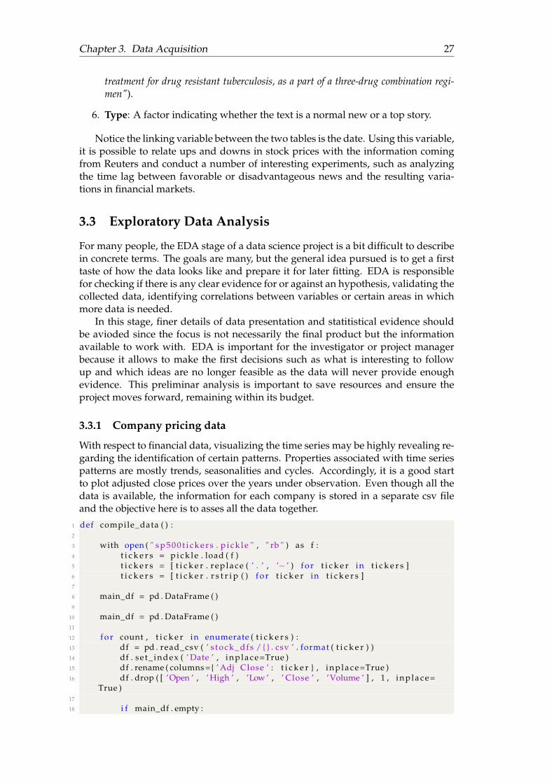
Chapter 3. Data Acquisition 27
treatment for drug resistant tuberculosis, as a part of a three-drug combination regi-men").
6. Type: A factor indicating whether the text is a normal new or a top story.
Notice the linking variable between the two tables is the date. Using this variable,it is possible to relate ups and downs in stock prices with the information comingfrom Reuters and conduct a number of interesting experiments, such as analyzingthe time lag between favorable or disadvantageous news and the resulting varia-tions in financial markets.
3.3 Exploratory Data Analysis
For many people, the EDA stage of a data science project is a bit difficult to describein concrete terms. The goals are many, but the general idea pursued is to get a firsttaste of how the data looks like and prepare it for later fitting. EDA is responsiblefor checking if there is any clear evidence for or against an hypothesis, validating thecollected data, identifying correlations between variables or certain areas in whichmore data is needed.
In this stage, finer details of data presentation and statitistical evidence shouldbe avioded since the focus is not necessarily the final product but the informationavailable to work with. EDA is important for the investigator or project managerbecause it allows to make the first decisions such as what is interesting to followup and which ideas are no longer feasible as the data will never provide enoughevidence. This preliminar analysis is important to save resources and ensure theproject moves forward, remaining within its budget.
3.3.1 Company pricing data
With respect to financial data, visualizing the time series may be highly revealing re-garding the identification of certain patterns. Properties associated with time seriespatterns are mostly trends, seasonalities and cycles. Accordingly, it is a good startto plot adjusted close prices over the years under observation. Even though all thedata is available, the information for each company is stored in a separate csv fileand the objective here is to asses all the data together.
1 def compile_data ( ) :2
3 with open ( " s p 5 0 0 t i c k e r s . p i c k l e " , " rb " ) as f :4 t i c k e r s = p i c k l e . load ( f )5 t i c k e r s = [ t i c k e r . r e p l a c e ( ’ . ’ , ’� ’ ) f o r t i c k e r in t i c k e r s ]6 t i c k e r s = [ t i c k e r . r s t r i p ( ) f o r t i c k e r in t i c k e r s ]7
8 main_df = pd . DataFrame ( )9
10 main_df = pd . DataFrame ( )11
12 f o r count , t i c k e r in enumerate ( t i c k e r s ) :13 df = pd . read_csv ( ’ s tock_dfs / { } . csv ’ . format ( t i c k e r ) )14 df . se t_ index ( ’ Date ’ , i n p l a c e=True )15 df . rename ( columns ={ ’ Adj Close ’ : t i c k e r } , i n p l a c e=True )16 df . drop ( [ ’Open ’ , ’ High ’ , ’Low ’ , ’ Close ’ , ’Volume ’ ] , 1 , i n p l a c e=
True )17
18 i f main_df . empty :
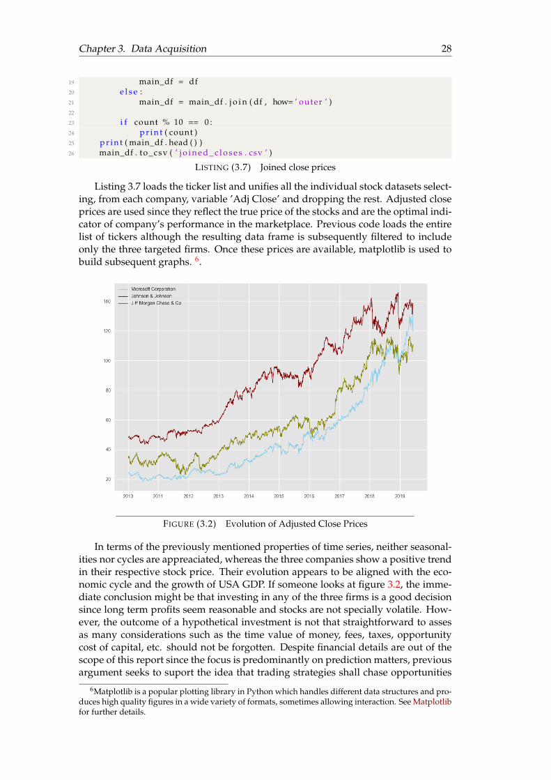
Chapter 3. Data Acquisition 28
19 main_df = df20 e l s e :21 main_df = main_df . j o i n ( df , how= ’ outer ’ )22
23 i f count % 10 == 0 :24 p r i n t ( count )25 p r i n t ( main_df . head ( ) )26 main_df . to_csv ( ’ j o i n e d _ c l o s e s . csv ’ )
LISTING (3.7) Joined close prices
Listing 3.7 loads the ticker list and unifies all the individual stock datasets select-ing, from each company, variable ’Adj Close’ and dropping the rest. Adjusted closeprices are used since they reflect the true price of the stocks and are the optimal indi-cator of company’s performance in the marketplace. Previous code loads the entirelist of tickers although the resulting data frame is subsequently filtered to includeonly the three targeted firms. Once these prices are available, matplotlib is used tobuild subsequent graphs. 6.
FIGURE (3.2) Evolution of Adjusted Close Prices
In terms of the previously mentioned properties of time series, neither seasonal-ities nor cycles are appreaciated, whereas the three companies show a positive trendin their respective stock price. Their evolution appears to be aligned with the eco-nomic cycle and the growth of USA GDP. If someone looks at figure 3.2, the imme-diate conclusion might be that investing in any of the three firms is a good decisionsince long term profits seem reasonable and stocks are not specially volatile. How-ever, the outcome of a hypothetical investment is not that straightforward to assesas many considerations such as the time value of money, fees, taxes, opportunitycost of capital, etc. should not be forgotten. Despite financial details are out of thescope of this report since the focus is predominantly on prediction matters, previousargument seeks to suport the idea that trading strategies shall chase opportunities
6Matplotlib is a popular plotting library in Python which handles different data structures and pro-duces high quality figures in a wide variety of formats, sometimes allowing interaction. See Matplotlibfor further details.
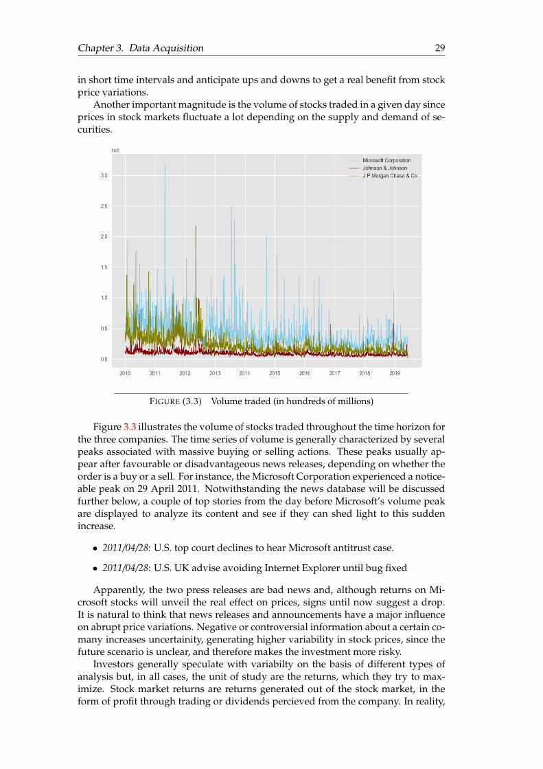
Chapter 3. Data Acquisition 29
in short time intervals and anticipate ups and downs to get a real benefit from stockprice variations.
Another important magnitude is the volume of stocks traded in a given day sinceprices in stock markets fluctuate a lot depending on the supply and demand of se-curities.
FIGURE (3.3) Volume traded (in hundreds of millions)
Figure 3.3 illustrates the volume of stocks traded throughout the time horizon forthe three companies. The time series of volume is generally characterized by severalpeaks associated with massive buying or selling actions. These peaks usually ap-pear after favourable or disadvantageous news releases, depending on whether theorder is a buy or a sell. For instance, the Microsoft Corporation experienced a notice-able peak on 29 April 2011. Notwithstanding the news database will be discussedfurther below, a couple of top stories from the day before Microsoft’s volume peakare displayed to analyze its content and see if they can shed light to this suddenincrease.
• 2011/04/28: U.S. top court declines to hear Microsoft antitrust case.
• 2011/04/28: U.S. UK advise avoiding Internet Explorer until bug fixed
Apparently, the two press releases are bad news and, although returns on Mi-crosoft stocks will unveil the real effect on prices, signs until now suggest a drop.It is natural to think that news releases and announcements have a major influenceon abrupt price variations. Negative or controversial information about a certain co-many increases uncertainity, generating higher variability in stock prices, since thefuture scenario is unclear, and therefore makes the investment more risky.
Investors generally speculate with variabilty on the basis of different types ofanalysis but, in all cases, the unit of study are the returns, which they try to max-imize. Stock market returns are returns generated out of the stock market, in theform of profit through trading or dividends percieved from the company. In reality,
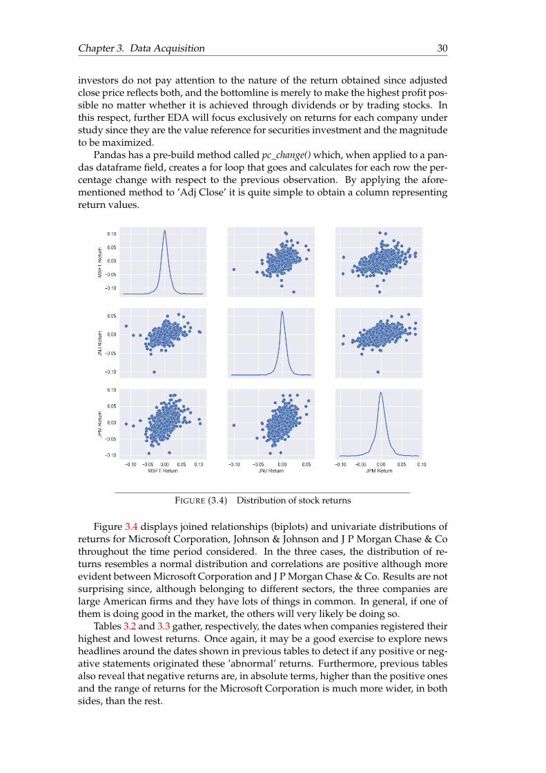
Chapter 3. Data Acquisition 30
investors do not pay attention to the nature of the return obtained since adjustedclose price reflects both, and the bottomline is merely to make the highest profit pos-sible no matter whether it is achieved through dividends or by trading stocks. Inthis respect, further EDA will focus exclusively on returns for each company understudy since they are the value reference for securities investment and the magnitudeto be maximized.
Pandas has a pre-build method called pc_change() which, when applied to a pan-das dataframe field, creates a for loop that goes and calculates for each row the per-centage change with respect to the previous observation. By applying the afore-mentioned method to ’Adj Close’ it is quite simple to obtain a column representingreturn values.
FIGURE (3.4) Distribution of stock returns
Figure 3.4 displays joined relationships (biplots) and univariate distributions ofreturns for Microsoft Corporation, Johnson & Johnson and J P Morgan Chase & Cothroughout the time period considered. In the three cases, the distribution of re-turns resembles a normal distribution and correlations are positive although moreevident between Microsoft Corporation and J P Morgan Chase & Co. Results are notsurprising since, although belonging to different sectors, the three companies arelarge American firms and they have lots of things in common. In general, if one ofthem is doing good in the market, the others will very likely be doing so.
Tables 3.2 and 3.3 gather, respectively, the dates when companies registered theirhighest and lowest returns. Once again, it may be a good exercise to explore newsheadlines around the dates shown in previous tables to detect if any positive or neg-ative statements originated these ’abnormal’ returns. Furthermore, previous tablesalso reveal that negative returns are, in absolute terms, higher than the positive onesand the range of returns for the Microsoft Corporation is much more wider, in bothsides, than the rest.
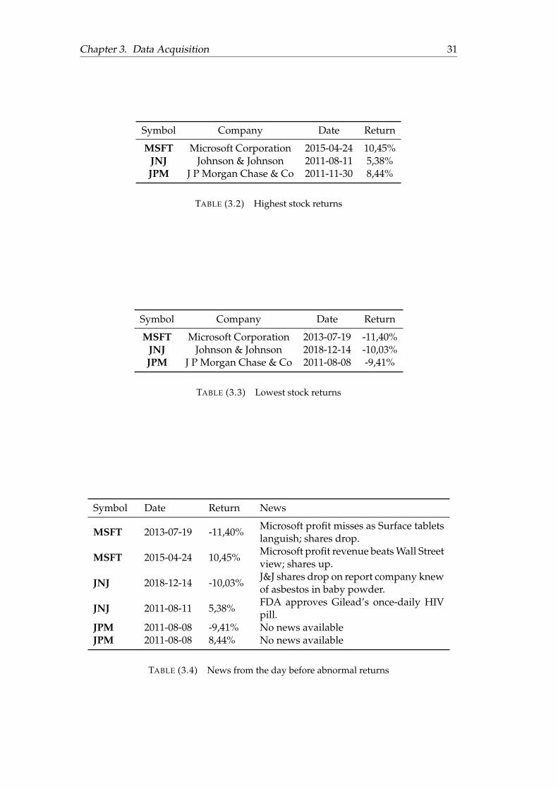
Chapter 3. Data Acquisition 31
Symbol Company Date Return
MSFT Microsoft Corporation 2015-04-24 10,45%JNJ Johnson & Johnson 2011-08-11 5,38%JPM J P Morgan Chase & Co 2011-11-30 8,44%
TABLE (3.2) Highest stock returns
Symbol Company Date Return
MSFT Microsoft Corporation 2013-07-19 -11,40%JNJ Johnson & Johnson 2018-12-14 -10,03%JPM J P Morgan Chase & Co 2011-08-08 -9,41%
TABLE (3.3) Lowest stock returns
Symbol Date Return News
MSFT 2013-07-19 -11,40% Microsoft profit misses as Surface tabletslanguish; shares drop.
MSFT 2015-04-24 10,45% Microsoft profit revenue beats Wall Streetview; shares up.
JNJ 2018-12-14 -10,03% J&J shares drop on report company knewof asbestos in baby powder.
JNJ 2011-08-11 5,38% FDA approves Gilead’s once-daily HIVpill.
JPM 2011-08-08 -9,41% No news availableJPM 2011-08-08 8,44% No news available
TABLE (3.4) News from the day before abnormal returns
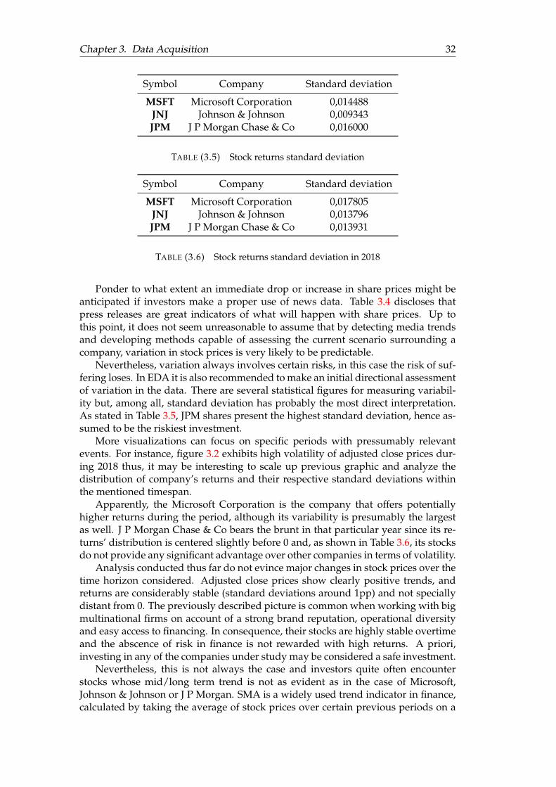
Chapter 3. Data Acquisition 32
Symbol Company Standard deviation
MSFT Microsoft Corporation 0,014488JNJ Johnson & Johnson 0,009343JPM J P Morgan Chase & Co 0,016000
TABLE (3.5) Stock returns standard deviation
Symbol Company Standard deviation
MSFT Microsoft Corporation 0,017805JNJ Johnson & Johnson 0,013796JPM J P Morgan Chase & Co 0,013931
TABLE (3.6) Stock returns standard deviation in 2018
Ponder to what extent an immediate drop or increase in share prices might beanticipated if investors make a proper use of news data. Table 3.4 discloses thatpress releases are great indicators of what will happen with share prices. Up tothis point, it does not seem unreasonable to assume that by detecting media trendsand developing methods capable of assessing the current scenario surrounding acompany, variation in stock prices is very likely to be predictable.
Nevertheless, variation always involves certain risks, in this case the risk of suf-fering loses. In EDA it is also recommended to make an initial directional assessmentof variation in the data. There are several statistical figures for measuring variabil-ity but, among all, standard deviation has probably the most direct interpretation.As stated in Table 3.5, JPM shares present the highest standard deviation, hence as-sumed to be the riskiest investment.
More visualizations can focus on specific periods with pressumably relevantevents. For instance, figure 3.2 exhibits high volatility of adjusted close prices dur-ing 2018 thus, it may be interesting to scale up previous graphic and analyze thedistribution of company’s returns and their respective standard deviations withinthe mentioned timespan.
Apparently, the Microsoft Corporation is the company that offers potentiallyhigher returns during the period, although its variability is presumably the largestas well. J P Morgan Chase & Co bears the brunt in that particular year since its re-turns’ distribution is centered slightly before 0 and, as shown in Table 3.6, its stocksdo not provide any significant advantage over other companies in terms of volatility.
Analysis conducted thus far do not evince major changes in stock prices over thetime horizon considered. Adjusted close prices show clearly positive trends, andreturns are considerably stable (standard deviations around 1pp) and not speciallydistant from 0. The previously described picture is common when working with bigmultinational firms on account of a strong brand reputation, operational diversityand easy access to financing. In consequence, their stocks are highly stable overtimeand the abscence of risk in finance is not rewarded with high returns. A priori,investing in any of the companies under study may be considered a safe investment.
Nevertheless, this is not always the case and investors quite often encounterstocks whose mid/long term trend is not as evident as in the case of Microsoft,Johnson & Johnson or J P Morgan. SMA is a widely used trend indicator in finance,calculated by taking the average of stock prices over certain previous periods on a
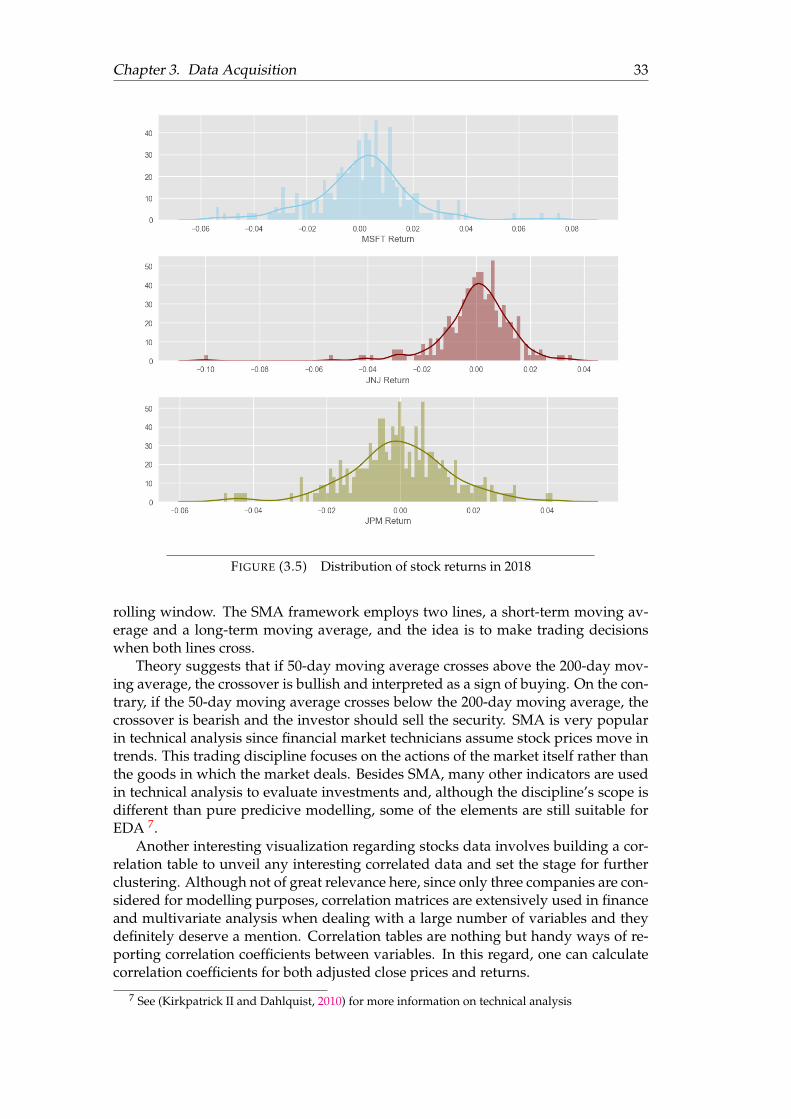
Chapter 3. Data Acquisition 33
FIGURE (3.5) Distribution of stock returns in 2018
rolling window. The SMA framework employs two lines, a short-term moving av-erage and a long-term moving average, and the idea is to make trading decisionswhen both lines cross.
Theory suggests that if 50-day moving average crosses above the 200-day mov-ing average, the crossover is bullish and interpreted as a sign of buying. On the con-trary, if the 50-day moving average crosses below the 200-day moving average, thecrossover is bearish and the investor should sell the security. SMA is very popularin technical analysis since financial market technicians assume stock prices move intrends. This trading discipline focuses on the actions of the market itself rather thanthe goods in which the market deals. Besides SMA, many other indicators are usedin technical analysis to evaluate investments and, although the discipline’s scope isdifferent than pure predicive modelling, some of the elements are still suitable forEDA 7.
Another interesting visualization regarding stocks data involves building a cor-relation table to unveil any interesting correlated data and set the stage for furtherclustering. Although not of great relevance here, since only three companies are con-sidered for modelling purposes, correlation matrices are extensively used in financeand multivariate analysis when dealing with a large number of variables and theydefinitely deserve a mention. Correlation tables are nothing but handy ways of re-porting correlation coefficients between variables. In this regard, one can calculatecorrelation coefficients for both adjusted close prices and returns.
7 See (Kirkpatrick II and Dahlquist, 2010) for more information on technical analysis
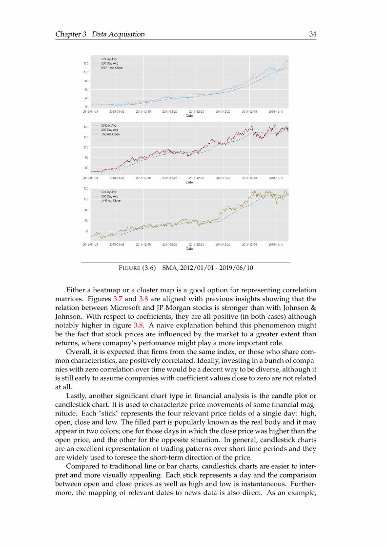
Chapter 3. Data Acquisition 34
FIGURE (3.6) SMA, 2012/01/01 - 2019/06/10
Either a heatmap or a cluster map is a good option for representing correlationmatrices. Figures 3.7 and 3.8 are aligned with previous insights showing that therelation between Microsoft and JP Morgan stocks is stronger than with Johnson &Johnson. With respect to coefficients, they are all positive (in both cases) althoughnotably higher in figure 3.8. A naive explanation behind this phenomenon mightbe the fact that stock prices are influenced by the market to a greater extent thanreturns, where comapny’s perfomance might play a more important role.
Overall, it is expected that firms from the same index, or those who share com-mon characteristics, are positively correlated. Ideally, investing in a bunch of compa-nies with zero correlation over time would be a decent way to be diverse, although itis still early to assume companies with coefficient values close to zero are not relatedat all.
Lastly, another significant chart type in financial analysis is the candle plot orcandlestick chart. It is used to characterize price movements of some financial mag-nitude. Each "stick" represents the four relevant price fields of a single day: high,open, close and low. The filled part is popularly known as the real body and it mayappear in two colors; one for those days in which the close price was higher than theopen price, and the other for the opposite situation. In general, candlestick chartsare an excellent representation of trading patterns over short time periods and theyare widely used to foresee the short-term direction of the price.
Compared to traditional line or bar charts, candlestick charts are easier to inter-pret and more visually appealing. Each stick represents a day and the comparisonbetween open and close prices as well as high and low is instantaneous. Further-more, the mapping of relevant dates to news data is also direct. As an example,
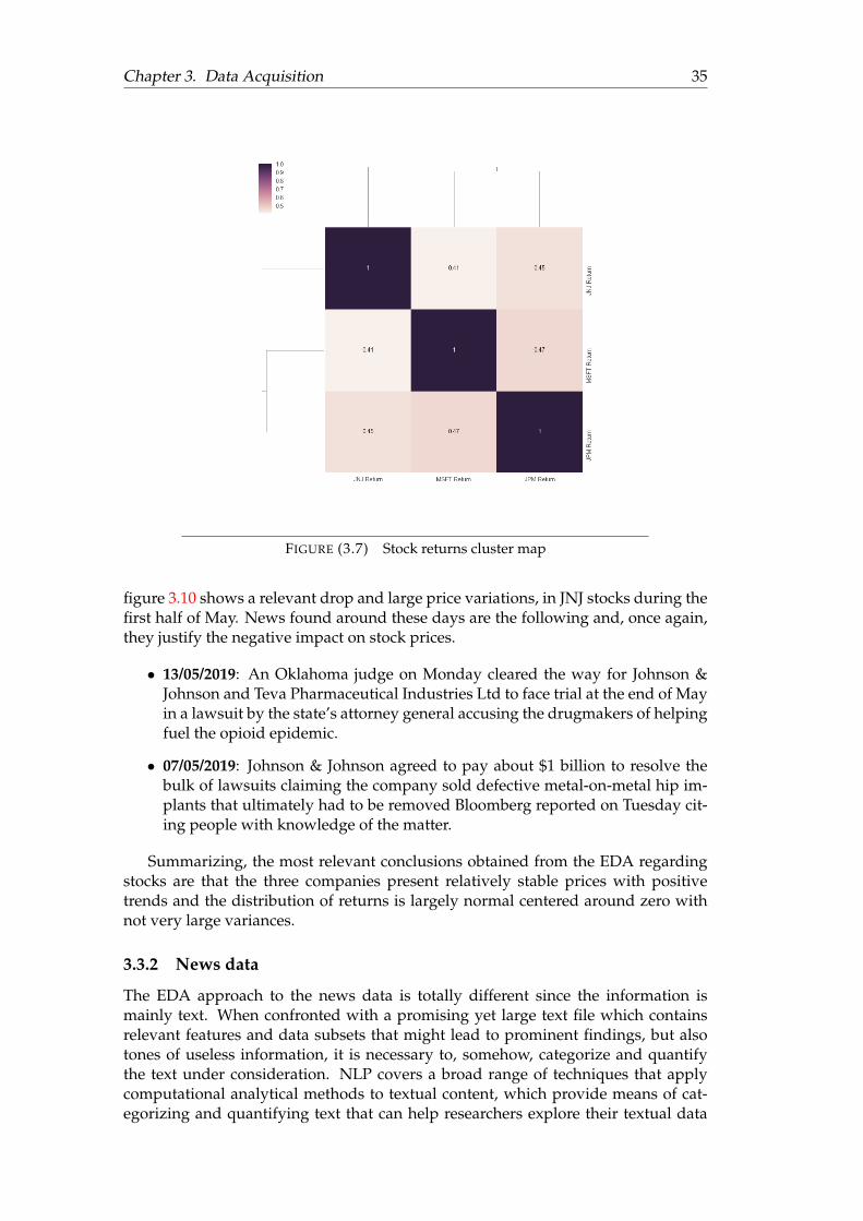
Chapter 3. Data Acquisition 35
FIGURE (3.7) Stock returns cluster map
figure 3.10 shows a relevant drop and large price variations, in JNJ stocks during thefirst half of May. News found around these days are the following and, once again,they justify the negative impact on stock prices.
• 13/05/2019: An Oklahoma judge on Monday cleared the way for Johnson &Johnson and Teva Pharmaceutical Industries Ltd to face trial at the end of Mayin a lawsuit by the state’s attorney general accusing the drugmakers of helpingfuel the opioid epidemic.
• 07/05/2019: Johnson & Johnson agreed to pay about $1 billion to resolve thebulk of lawsuits claiming the company sold defective metal-on-metal hip im-plants that ultimately had to be removed Bloomberg reported on Tuesday cit-ing people with knowledge of the matter.
Summarizing, the most relevant conclusions obtained from the EDA regardingstocks are that the three companies present relatively stable prices with positivetrends and the distribution of returns is largely normal centered around zero withnot very large variances.
3.3.2 News data
The EDA approach to the news data is totally different since the information ismainly text. When confronted with a promising yet large text file which containsrelevant features and data subsets that might lead to prominent findings, but alsotones of useless information, it is necessary to, somehow, categorize and quantifythe text under consideration. NLP covers a broad range of techniques that applycomputational analytical methods to textual content, which provide means of cat-egorizing and quantifying text that can help researchers explore their textual data
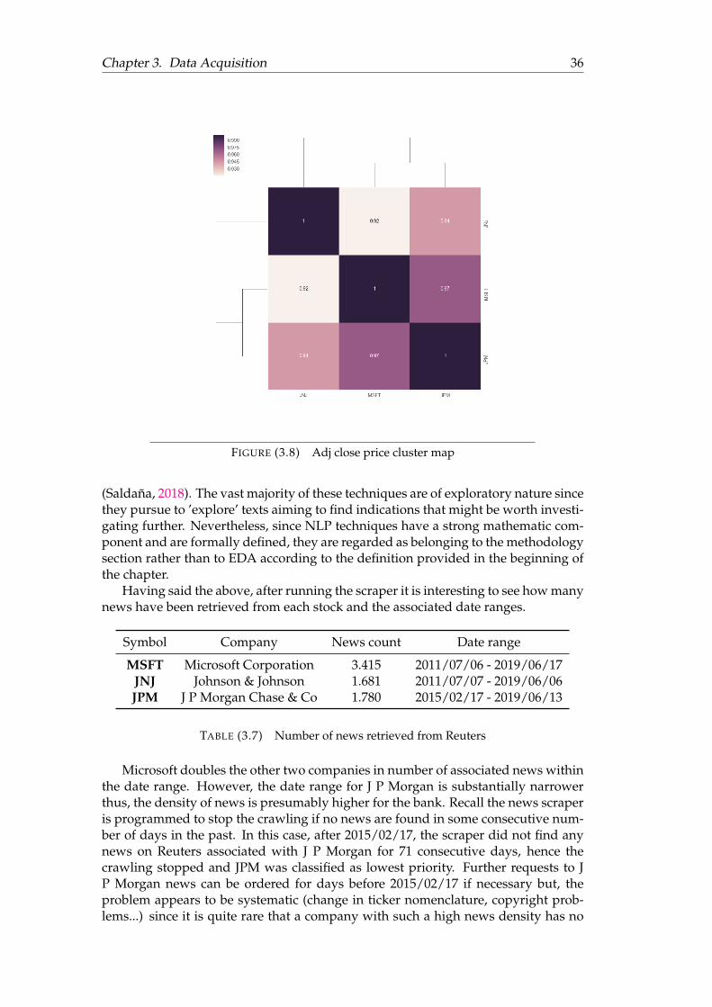
Chapter 3. Data Acquisition 36
FIGURE (3.8) Adj close price cluster map
(Saldaña, 2018). The vast majority of these techniques are of exploratory nature sincethey pursue to ’explore’ texts aiming to find indications that might be worth investi-gating further. Nevertheless, since NLP techniques have a strong mathematic com-ponent and are formally defined, they are regarded as belonging to the methodologysection rather than to EDA according to the definition provided in the beginning ofthe chapter.
Having said the above, after running the scraper it is interesting to see how manynews have been retrieved from each stock and the associated date ranges.
Symbol Company News count Date range
MSFT Microsoft Corporation 3.415 2011/07/06 - 2019/06/17JNJ Johnson & Johnson 1.681 2011/07/07 - 2019/06/06JPM J P Morgan Chase & Co 1.780 2015/02/17 - 2019/06/13
TABLE (3.7) Number of news retrieved from Reuters
Microsoft doubles the other two companies in number of associated news withinthe date range. However, the date range for J P Morgan is substantially narrowerthus, the density of news is presumably higher for the bank. Recall the news scraperis programmed to stop the crawling if no news are found in some consecutive num-ber of days in the past. In this case, after 2015/02/17, the scraper did not find anynews on Reuters associated with J P Morgan for 71 consecutive days, hence thecrawling stopped and JPM was classified as lowest priority. Further requests to JP Morgan news can be ordered for days before 2015/02/17 if necessary but, theproblem appears to be systematic (change in ticker nomenclature, copyright prob-lems...) since it is quite rare that a company with such a high news density has no
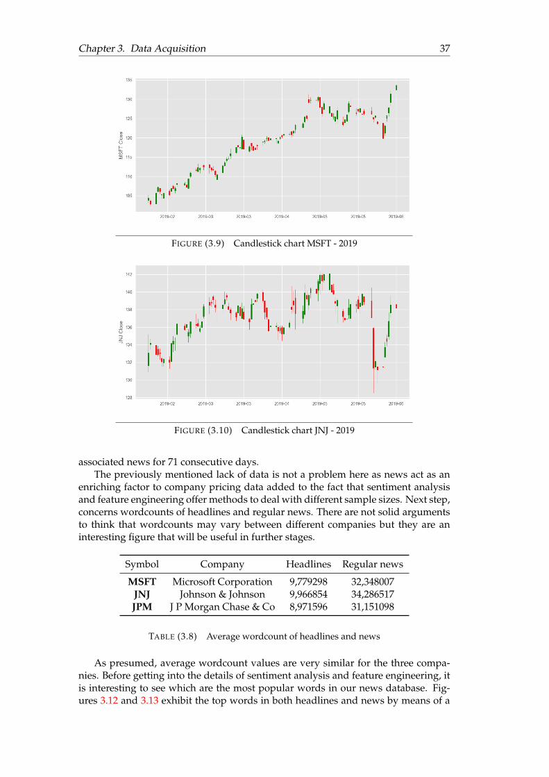
Chapter 3. Data Acquisition 37
FIGURE (3.9) Candlestick chart MSFT - 2019
FIGURE (3.10) Candlestick chart JNJ - 2019
associated news for 71 consecutive days.The previously mentioned lack of data is not a problem here as news act as an
enriching factor to company pricing data added to the fact that sentiment analysisand feature engineering offer methods to deal with different sample sizes. Next step,concerns wordcounts of headlines and regular news. There are not solid argumentsto think that wordcounts may vary between different companies but they are aninteresting figure that will be useful in further stages.
Symbol Company Headlines Regular news
MSFT Microsoft Corporation 9,779298 32,348007JNJ Johnson & Johnson 9,966854 34,286517JPM J P Morgan Chase & Co 8,971596 31,151098
TABLE (3.8) Average wordcount of headlines and news
As presumed, average wordcount values are very similar for the three compa-nies. Before getting into the details of sentiment analysis and feature engineering, itis interesting to see which are the most popular words in our news database. Fig-ures 3.12 and 3.13 exhibit the top words in both headlines and news by means of a
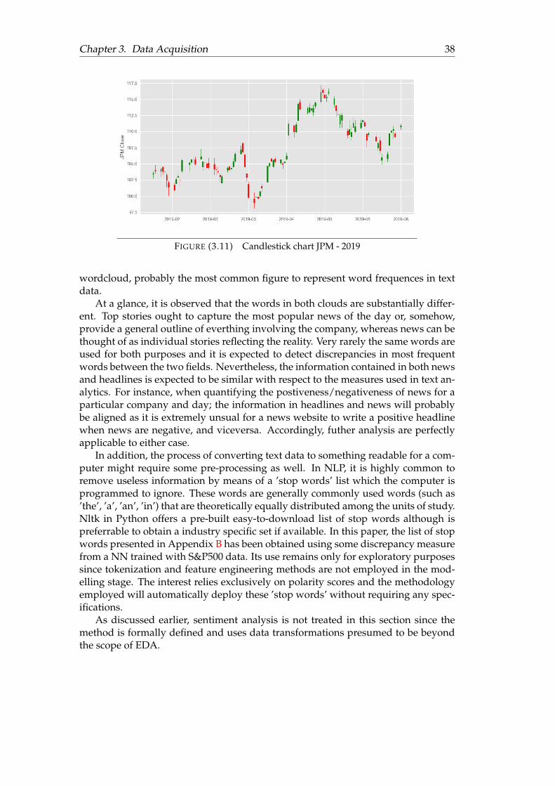
Chapter 3. Data Acquisition 38
FIGURE (3.11) Candlestick chart JPM - 2019
wordcloud, probably the most common figure to represent word frequences in textdata.
At a glance, it is observed that the words in both clouds are substantially differ-ent. Top stories ought to capture the most popular news of the day or, somehow,provide a general outline of everthing involving the company, whereas news can bethought of as individual stories reflecting the reality. Very rarely the same words areused for both purposes and it is expected to detect discrepancies in most frequentwords between the two fields. Nevertheless, the information contained in both newsand headlines is expected to be similar with respect to the measures used in text an-alytics. For instance, when quantifying the postiveness/negativeness of news for aparticular company and day; the information in headlines and news will probablybe aligned as it is extremely unsual for a news website to write a positive headlinewhen news are negative, and viceversa. Accordingly, futher analysis are perfectlyapplicable to either case.
In addition, the process of converting text data to something readable for a com-puter might require some pre-processing as well. In NLP, it is highly common toremove useless information by means of a ’stop words’ list which the computer isprogrammed to ignore. These words are generally commonly used words (such as’the’, ’a’, ’an’, ’in’) that are theoretically equally distributed among the units of study.Nltk in Python offers a pre-built easy-to-download list of stop words although ispreferrable to obtain a industry specific set if available. In this paper, the list of stopwords presented in Appendix B has been obtained using some discrepancy measurefrom a NN trained with S&P500 data. Its use remains only for exploratory purposessince tokenization and feature engineering methods are not employed in the mod-elling stage. The interest relies exclusively on polarity scores and the methodologyemployed will automatically deploy these ’stop words’ without requiring any spec-ifications.
As discussed earlier, sentiment analysis is not treated in this section since themethod is formally defined and uses data transformations presumed to be beyondthe scope of EDA.
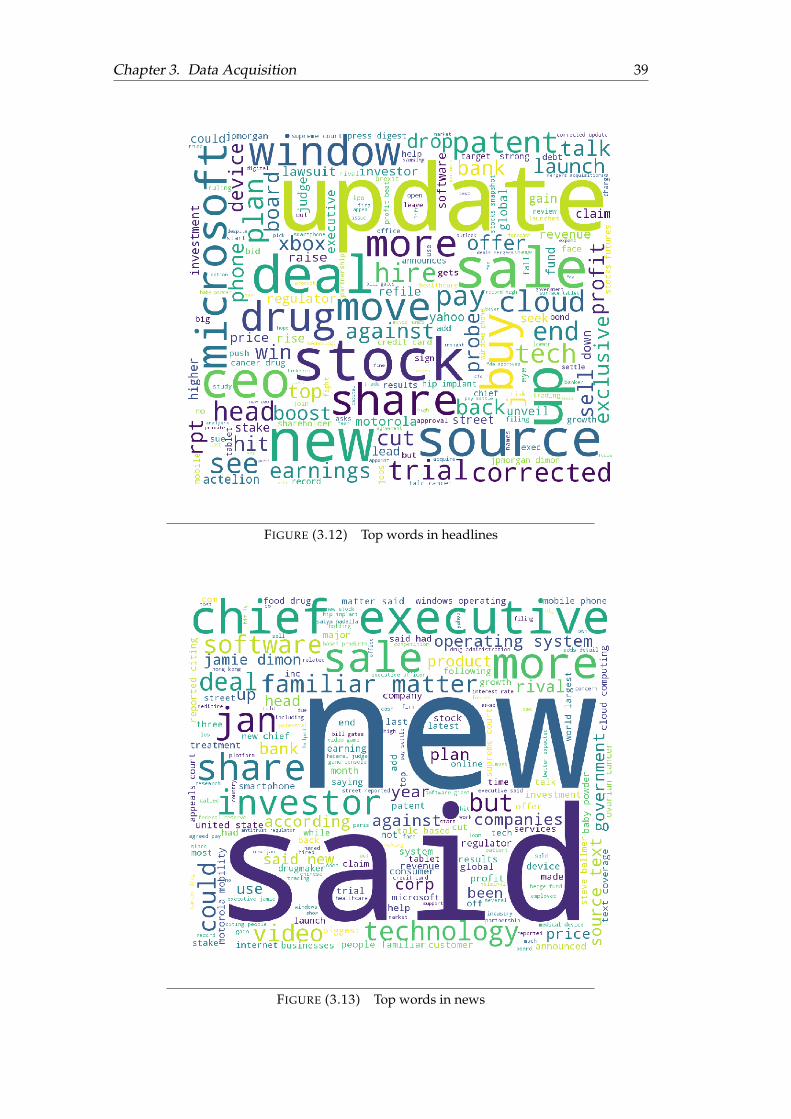
Chapter 3. Data Acquisition 39
FIGURE (3.12) Top words in headlines
FIGURE (3.13) Top words in news
40
Chapter 4
Methods
The question raised in this paper is mainly of predictive nature. One of the major ob-jectives pursued, besides automating the data obtenion process, involves being ableto cast future stock prices of companies using time series of financial data and infor-mation from news on Reuters. Notwithstanding the theoretical nature of the study,the capacity of anticipating future ups and downs in securities’ price is a preciousresource that many companies use to get profits in stock markets or make businesswith it.
Traditionally, financial analysis has been highly based on a large list of financialindicators and data taken from financial statements. Accounting ratios, percentageof inter-firm comparison, intra-firm comparison, common size statement, etc., werevery popular figures employed to ascertain relationships between internal account-ing magnitudes and what was happening in the market. Even though these methodsallow some space for certain mathematical modelling, the approach was still highlytheoretical-based and strongly rooted in economic theory.
In recent years though, Machine learning and Deep leaning have proven to beeffective strategies to maximize profits in financial markets. The approach is com-pletely different since financial statements are no longer contemplated and the focusnow is on the alternative sources of information which provide additional insightsto capture drivers outside the scope of economic theory but still influential in stockmarkets. Finance is highly nonlinear and some theorists even believe price move-ments are completely random. In 1973 professor Burton Gordon Malkiel publishedhis famous ’Random Walk Down Wall Street’, one of the most famous experimentsabout the reliability of investments made by stock market analysts. In his book,Malkiel compared an investment guided by professionals with another made com-pletely at random, precisely, he used as a figure of speech, a blinded monkey throw-ing darts to a wall street newspaper with stock names. Surprisingly, the monkey’sportfolio got higher returns than 85% of professional investors in addition to exceed-ing returns achieved by the main indexes. By that time, traditional time series meth-ods like ARIMA or GARCH models were the dominant note in the industry, andthese methods are effective only when the series is stationary. Stationarity of timeseries is a restricting assumption that requires data to be preprocessed by taking logreturns (or other transformations). Furthermore, even if the data shows certain sta-tionarity, in a live trading system there is no guarantee of stationarity as new datais added. Neural Networks partially resolve the stationarity problem as they do notrequire any data assumptions and, as discussed in chapter 1, they are also very goodat finding patterns out of raw data.
Flexibility and non-linearity are probably the most powerful characteristics ofneural networks. They do not require any data assumption and are capable of ap-proximating practically anything that can be turned into a number. Another im-portant feature of neural networks is their adaptive feature/basis structure which
Chapter 4. Methods 41
enables them to face problems with many inputs and high dimensionality, such asimages. Futhermore, even though the training can be tedious, once finished, pre-dictions are instantaneous. On the other hand, likelihood functions are no longer aconvex function of the model parameters hence the problem might become to expen-sive and time consuming to train with traditional CPUs. In addition, overfitting andgeneralization problems are very likely to appear, specially in data scarce scenarios.
The methodology employed in this paper is strongly based on Deep Learningand Neural Networks seeking to turn a financial/economic problem into pure pre-dictive modelling and forget about any data assumption which is out of our control.The hypothesis raised pretends to test if time series modelling of financial data canbe enriched using news’ sentiments. Some neural networks achieved significant re-sults in time series prediction of financial data, although the methods employed areextension of regression algorithms that can only handle quantitative variables. Ac-cordingly, the inclusion of any kind of sentiment magnitude in these models hasbeen a real challenge still unresolved. The common approach to stock price predic-tion using news data is slightly different as it generally uses classification algorithmson labelled data and the predictions are predominantly buy or sell signals. On theoccasion of the recent emergence of VADER sentiment analysis, a method capable ofassigning quantifiable sentiment scores to text data, this study aims to test whetherthe VADER methodology has practical applications on the modelling of financialtime series from a regression perspective, essentially acting as an enriching factor toother quantitative magnitudes considered.
Firstly, to turn news data into something a computer can understand and usewhen training the network, VADER sentiment analysis is conducted to assign a sen-timent score to each new in the dataset. Subsequently, company price data is mergedwith the previously obtained scores by date, and different models are fitted. There isstill litte theory behind deep learning models hence highly difficult to find answersto questions like: which NN architecture is the best for this problem, what is theoptimal number of epochs/layers or which activation functions should be consid-ered. Sometimes NN design is more an art than a science, with trial and error as thebest option to assess a model’s performance. Accordingly, the models built seek toprovide the reader with certain educated guesses that might be of practical utility inthe industry based on previous empirical evidence.
4.1 Theoretical considerations
Neural Networks are a relatively new instrument in scientific computing and theyoffer many advantages over traditional inferential methods, some of them alreadydiscussed. However, it is also important to be concerned about their limitations andthe theoretical basis behind. Some of the most important ones are presented below.
4.1.1 Universal approximation theorem
The universal appoximation theorem lays the mathematical foundations of artificialneural networks by stating that a feed-forward network (no cycles) with a singlehidden layer containing a finite number of neurons can approximate continuousfunctions on compact subsets of Rn.
One of the first versions of the theorem was developed by (Cybenko, 1989) forsigmoid activation functions.
Chapter 4. Methods 42
Theorem 1. Let s be any continous discriminatory function. Then finite sums of theform:
G(x) =N
Âj=1
ajs⇣
yTj x + qj
⌘(4.1)
are dense in C(In). In other words, given any f 2 C(In) and e > 0, there is a sum,G(x) of the above for which
|G(x)� f (x)| < e, for all x 2 In
Previous expression clearly resembles the mathematical representation of an arti-ficial neuron in 1.1. Later proofs demonstrate the equality still holds when replacinge with any general nonconstant, bounded and continuous function: j : R ! R.
In 2017, Hanin improved previous result 4.1 showing that ReLU neural networkswith width n + 1 are sufficient to approximate any continuous convex function of n-dimensional input variables (Hanin, 2017).
Theorem 2. For any Lebesgue-integrable function f : Rn ! R satisfying {x : f (x) 6= 0}is a positive measure set in Lebesgue measure, and any function FA represented by a fully-connected ReLU network A with width dm n, the following equality holds:
Z
Rn| f (x)� FA(x)|dx = +•
Z
Rn| f (x)|dx (4.2)
The evolution of the universal approximation theorem throught the last 20 yearsis a strong argument for believing that neural networks are capable of approximatingpractically anything that can be turned into a quantifiable magnitude without anydata assumptions.
4.1.2 Activation functions
In the flow of a network, as its name suggests, the activation function is responsiblefor deciding whether the neuron is ’firing’ or not. Consider the neuron in 1.1. Itbasically calculates a weighted sum of its input, adds a bias, and function q decideswhether it should be active or not.
The value of xi[t] can be anything in the range (�•,+•) as the neuron itselfdoes not stablish any bounds of the output. Activation functions are added to assessthe value produced by a neuron and decide whether outside connections shouldconsider this neuron as ’activated’ or not.
First thing that might come to someone’s mind is a threshold based step functionto discriminate between active and inactive neurons. Something such as f (xi[t]) = 1,hence ’activated’ if xi[t] > threshold, and f (xi[t]) = 0 otherwise, is very intuitive andeven of practical utility for a binary problem. However, when facing a multi-classclassification problem or a continous target, step functions have various limitationsas a 0/1 ouput does not say much about results the network is trying to predict. Inthis situations, it is better to obtain a range of activations and dedice which neuronsare firing by taking the max (or softmax) among, for instance, the values of thosesets of connected neurons where at least one is supposedly firing. This lead us toconclude that, in theory q can be any function since the operation is just a mappingof the resulting values into some domain where max or softmax functions can belater applied.
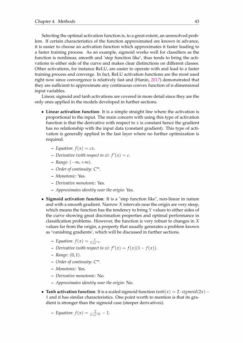
Chapter 4. Methods 43
Selecting the optimal activation function is, to a great extent, an unresolved prob-lem. If certain characteristics of the function approximated are known in advance,it is easier to choose an activation function which approximates it faster leading toa faster training process. As an example, sigmoid works well for classifiers as thefunction is nonlinear, smooth and ’step function like’, thus tends to bring the acti-vations to either side of the curve and makes clear distinctions on different classes.Other activations, for instance ReLU, are easier to operate with and lead to a fastertraining process and converge. In fact, ReLU activation functions are the most usedright now since convergence is relatively fast and (Hanin, 2017) demonstrated thatthey are sufficient to approximate any continuous convex function of n-dimensionalinput variables.
Linear, sigmoid and tanh activations are covered in more detail since they are theonly ones applied in the models developed in further sections.
• Linear activation function: It is a simple straight line where the activation isproportional to the input. The main concern with using this type of activationfunction is that the derivative with respect to x is constant hence the gradienthas no relationship with the input data (constant gradient). This type of acti-vation is generally applied in the last layer where no further optimization isrequired.
– Equation: f (x) = cx.– Derivative (with respect to x): f 0(x) = c.– Range: (�•,+•).– Order of continuity: C•.– Monotonic: Yes.– Derivative monotonic: Yes.– Approximates identity near the origin: Yes.
• Sigmoid activation function: It is a "step function like", non-linear in natureand with a smooth gradient. Narrow X intervals near the origin are very steep,which means the function has the tendency to bring Y values to either sides ofthe curve showing great discrimation properties and optimal performance inclassification problems. However, the function is very robust to changes in Xvalues far from the origin, a property that usually generates a problem knownas ’vanishing gradients’, which will be discussed in further sections.
– Equation: f (x) = 11+e�x .
– Derivative (with respect to x): f 0(x) = f (x)(1 � f (x)).– Range: (0, 1).– Order of continuity: C•.– Monotonic: Yes.– Derivative monotonic: No.– Approximates identity near the origin: No.
• Tanh activation function: It is a scaled sigmoid function tanh(x) = 2 · sigmoid(2x)�1 and it has similar characteristics. One point worth to mention is that its gra-dient is stronger than the sigmoid case (steeper derivatives).
– Equation: f (x) = 21+e�2x � 1.
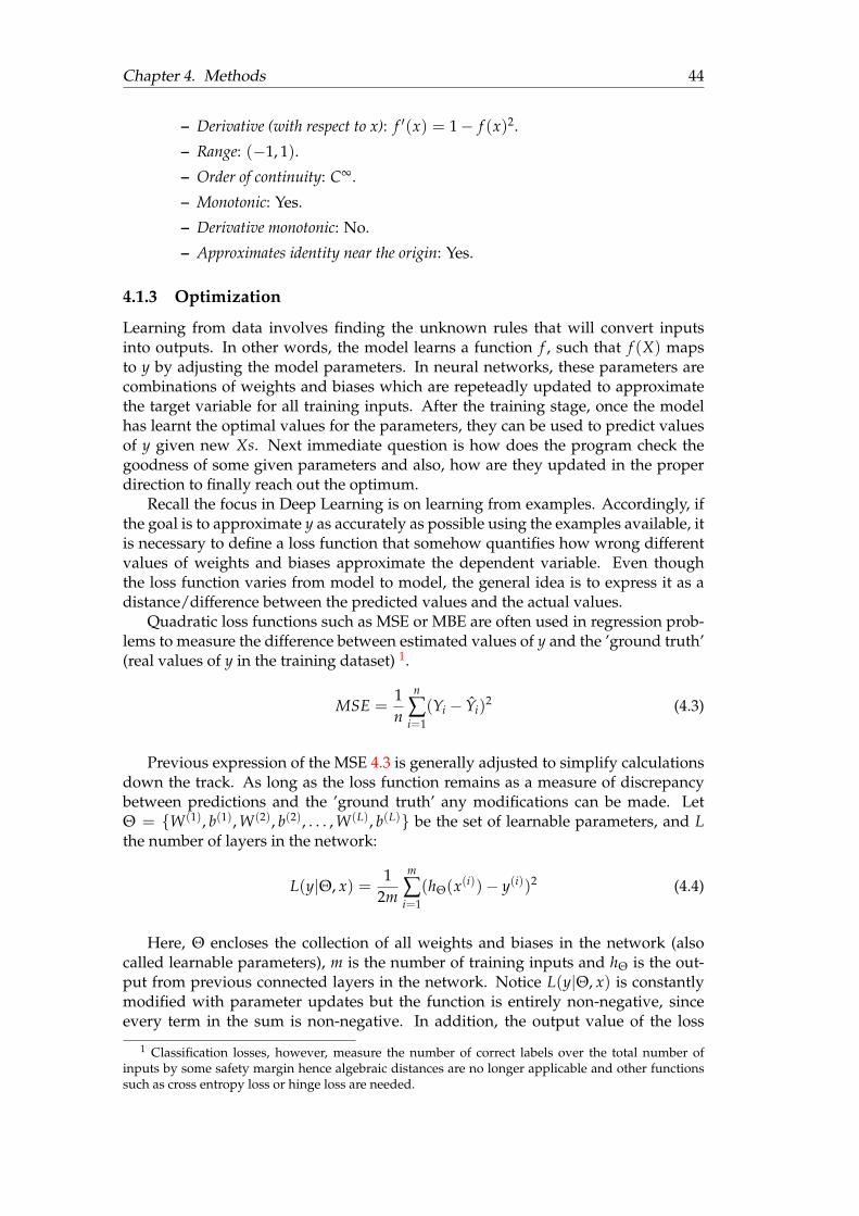
Chapter 4. Methods 44
– Derivative (with respect to x): f 0(x) = 1 � f (x)2.– Range: (�1, 1).– Order of continuity: C•.– Monotonic: Yes.– Derivative monotonic: No.– Approximates identity near the origin: Yes.
4.1.3 Optimization
Learning from data involves finding the unknown rules that will convert inputsinto outputs. In other words, the model learns a function f , such that f (X) mapsto y by adjusting the model parameters. In neural networks, these parameters arecombinations of weights and biases which are repeteadly updated to approximatethe target variable for all training inputs. After the training stage, once the modelhas learnt the optimal values for the parameters, they can be used to predict valuesof y given new Xs. Next immediate question is how does the program check thegoodness of some given parameters and also, how are they updated in the properdirection to finally reach out the optimum.
Recall the focus in Deep Learning is on learning from examples. Accordingly, ifthe goal is to approximate y as accurately as possible using the examples available, itis necessary to define a loss function that somehow quantifies how wrong differentvalues of weights and biases approximate the dependent variable. Even thoughthe loss function varies from model to model, the general idea is to express it as adistance/difference between the predicted values and the actual values.
Quadratic loss functions such as MSE or MBE are often used in regression prob-lems to measure the difference between estimated values of y and the ’ground truth’(real values of y in the training dataset) 1.
MSE =1n
n
Âi=1
(Yi � Yi)2 (4.3)
Previous expression of the MSE 4.3 is generally adjusted to simplify calculationsdown the track. As long as the loss function remains as a measure of discrepancybetween predictions and the ’ground truth’ any modifications can be made. LetQ = {W(1), b(1), W(2), b(2), . . . , W(L), b(L)} be the set of learnable parameters, and Lthe number of layers in the network:
L(y|Q, x) =1
2m
m
Âi=1
(hQ(x(i))� y(i))2 (4.4)
Here, Q encloses the collection of all weights and biases in the network (alsocalled learnable parameters), m is the number of training inputs and hQ is the out-put from previous connected layers in the network. Notice L(y|Q, x) is constantlymodified with parameter updates but the function is entirely non-negative, sinceevery term in the sum is non-negative. In addition, the output value of the loss
1 Classification losses, however, measure the number of correct labels over the total number ofinputs by some safety margin hence algebraic distances are no longer applicable and other functionssuch as cross entropy loss or hinge loss are needed.
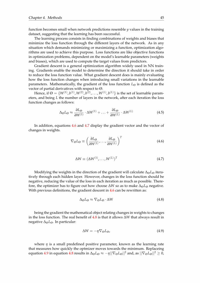
Chapter 4. Methods 45
function becomes small when network predictions resemble y values in the trainingdataset, suggesting that the learning has been successful.
The learning process consists in finding combinations of weights and biases thatminimize the loss function through the different layers of the network. As in anysituation which demands minimizing or maximizing a function, optimization algo-rithms are used to achieve this purpose. Loss functions are like objective functionsin optimization problems, dependent on the model’s learnable parameters (weightsand biases), which are used to compute the target values from predictors.
Gradient descent is a general optimization algorithm widely used in NN train-ing. Gradients enable the model to determine the direction it should take in orderto reduce the loss function value. What gradient descent does is mainly evaluatinghow the loss function changes when introducing small variations in the learnableparameters. Mathematically, the gradient of the loss function LQ is defined as thevector of partial derivatives with respect to Q.
Hence, if Q = {W(1), b(1), W(2), b(2), . . . , W(L), b(L)} is the set of learnable param-eters, and being L the number of layers in the network, after each iteration the lossfunction changes as follows:
DQLQ ⇡ ∂LQ
∂W(1) · DW(1) + . . . +∂LQ
∂W(L) · DW(L) (4.5)
In addition, equations 4.6 and 4.7 display the gradient vector and the vector ofchanges in weights.
rQLQ ⌘✓
∂LQ
∂W(1) , . . . ,∂LQ
∂W(L)
◆T(4.6)
DW ⌘ (DW(1), . . . , W(L))T (4.7)
Modifying the weights in the direction of the gradient will calculate DQLQ itera-tively through each hidden layer. However, changes in the loss function should benegative, reducing the value of the loss in each iteration as much as possible. There-fore, the optimizer has to figure out how choose DW so as to make DQLQ negative.With previous definitions, the gradient descent in 4.6 can be rewritten as:
DQLQ ⇡ rQLQ · DW (4.8)
being the gradient the mathematical object relating changes in weights to changesin the loss function. The real benefit of 4.8 is that it allows DW that always result innegative DQLQ. In particular:
DW = �hrQLQ, (4.9)
where h is a small predefined positive parameter, known as the learning ratethat measures how quickly the optmizer moves towards the minimum. Replaceingequation 4.9 in equation 4.8 results in DQLQ ⇡ �h||rQLQ||2 and, as ||rQLQ||2 � 0,
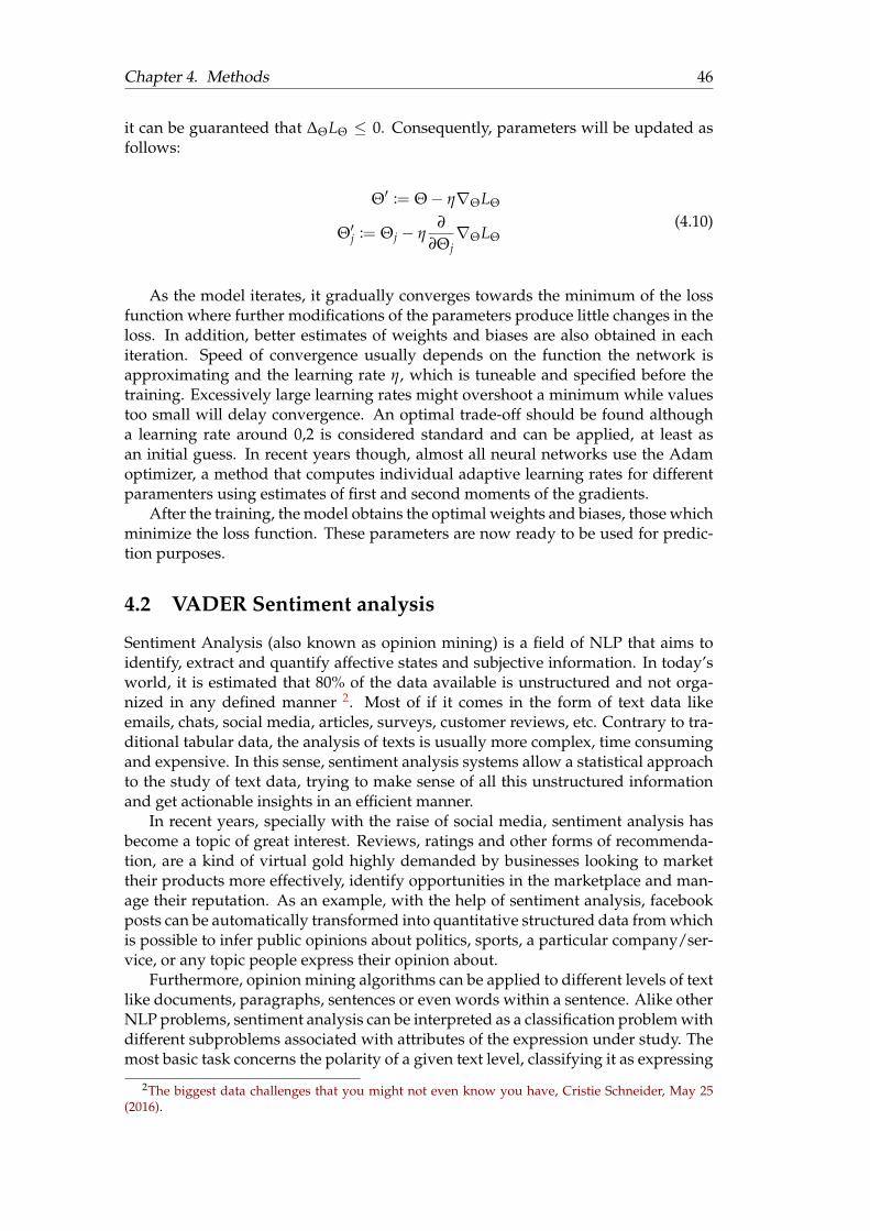
Chapter 4. Methods 46
it can be guaranteed that DQLQ 0. Consequently, parameters will be updated asfollows:
Q0 := Q � hrQLQ
Q0j := Qj � h
∂
∂QjrQLQ
(4.10)
As the model iterates, it gradually converges towards the minimum of the lossfunction where further modifications of the parameters produce little changes in theloss. In addition, better estimates of weights and biases are also obtained in eachiteration. Speed of convergence usually depends on the function the network isapproximating and the learning rate h, which is tuneable and specified before thetraining. Excessively large learning rates might overshoot a minimum while valuestoo small will delay convergence. An optimal trade-off should be found althougha learning rate around 0,2 is considered standard and can be applied, at least asan initial guess. In recent years though, almost all neural networks use the Adamoptimizer, a method that computes individual adaptive learning rates for differentparamenters using estimates of first and second moments of the gradients.
After the training, the model obtains the optimal weights and biases, those whichminimize the loss function. These parameters are now ready to be used for predic-tion purposes.
4.2 VADER Sentiment analysis
Sentiment Analysis (also known as opinion mining) is a field of NLP that aims toidentify, extract and quantify affective states and subjective information. In today’sworld, it is estimated that 80% of the data available is unstructured and not orga-nized in any defined manner 2. Most of if it comes in the form of text data likeemails, chats, social media, articles, surveys, customer reviews, etc. Contrary to tra-ditional tabular data, the analysis of texts is usually more complex, time consumingand expensive. In this sense, sentiment analysis systems allow a statistical approachto the study of text data, trying to make sense of all this unstructured informationand get actionable insights in an efficient manner.
In recent years, specially with the raise of social media, sentiment analysis hasbecome a topic of great interest. Reviews, ratings and other forms of recommenda-tion, are a kind of virtual gold highly demanded by businesses looking to markettheir products more effectively, identify opportunities in the marketplace and man-age their reputation. As an example, with the help of sentiment analysis, facebookposts can be automatically transformed into quantitative structured data from whichis possible to infer public opinions about politics, sports, a particular company/ser-vice, or any topic people express their opinion about.
Furthermore, opinion mining algorithms can be applied to different levels of textlike documents, paragraphs, sentences or even words within a sentence. Alike otherNLP problems, sentiment analysis can be interpreted as a classification problem withdifferent subproblems associated with attributes of the expression under study. Themost basic task concerns the polarity of a given text level, classifying it as expressing
2The biggest data challenges that you might not even know you have, Cristie Schneider, May 25(2016).
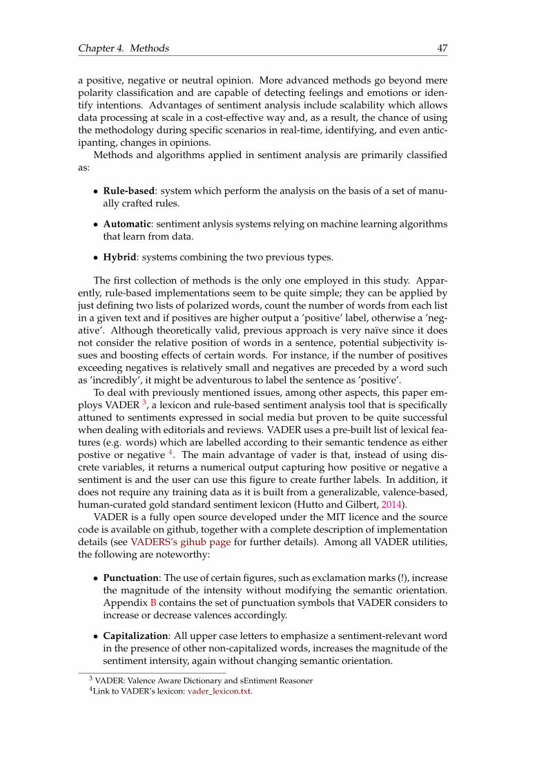
Chapter 4. Methods 47
a positive, negative or neutral opinion. More advanced methods go beyond merepolarity classification and are capable of detecting feelings and emotions or iden-tify intentions. Advantages of sentiment analysis include scalability which allowsdata processing at scale in a cost-effective way and, as a result, the chance of usingthe methodology during specific scenarios in real-time, identifying, and even antic-ipanting, changes in opinions.
Methods and algorithms applied in sentiment analysis are primarily classifiedas:
• Rule-based: system which perform the analysis on the basis of a set of manu-ally crafted rules.
• Automatic: sentiment anlysis systems relying on machine learning algorithmsthat learn from data.
• Hybrid: systems combining the two previous types.
The first collection of methods is the only one employed in this study. Appar-ently, rule-based implementations seem to be quite simple; they can be applied byjust defining two lists of polarized words, count the number of words from each listin a given text and if positives are higher output a ’positive’ label, otherwise a ’neg-ative’. Although theoretically valid, previous approach is very naïve since it doesnot consider the relative position of words in a sentence, potential subjectivity is-sues and boosting effects of certain words. For instance, if the number of positivesexceeding negatives is relatively small and negatives are preceded by a word suchas ’incredibly’, it might be adventurous to label the sentence as ’positive’.
To deal with previously mentioned issues, among other aspects, this paper em-ploys VADER 3, a lexicon and rule-based sentiment analysis tool that is specificallyattuned to sentiments expressed in social media but proven to be quite successfulwhen dealing with editorials and reviews. VADER uses a pre-built list of lexical fea-tures (e.g. words) which are labelled according to their semantic tendence as eitherpostive or negative 4. The main advantage of vader is that, instead of using dis-crete variables, it returns a numerical output capturing how positive or negative asentiment is and the user can use this figure to create further labels. In addition, itdoes not require any training data as it is built from a generalizable, valence-based,human-curated gold standard sentiment lexicon (Hutto and Gilbert, 2014).
VADER is a fully open source developed under the MIT licence and the sourcecode is available on github, together with a complete description of implementationdetails (see VADERS’s gihub page for further details). Among all VADER utilities,the following are noteworthy:
• Punctuation: The use of certain figures, such as exclamation marks (!), increasethe magnitude of the intensity without modifying the semantic orientation.Appendix B contains the set of punctuation symbols that VADER considers toincrease or decrease valences accordingly.
• Capitalization: All upper case letters to emphasize a sentiment-relevant wordin the presence of other non-capitalized words, increases the magnitude of thesentiment intensity, again without changing semantic orientation.
3 VADER: Valence Aware Dictionary and sEntiment Reasoner4Link to VADER’s lexicon: vader_lexicon.txt.
Chapter 4. Methods 48
• Boosters: Booster dictionary listed in Appendix B includes intensifiers whichimpact the sentiment intensity by either increasing or decreasing the inten-sity. For instance words such as extremely, absolutely or highly have a positiveimpact on sentiment scores while partly, occasionally or little contribute nega-tively.
• Conjunctions: Words expressing contrast like ’but’ suggest a shift in sentimentpolarity, with the sentiment of the text following the conjunction being domi-nant. For instance, a sentence such as: "The place was good but, the weatherwas horrible" will be classified as negative.
• Preceeding tri-gram: It is believed that by examining the word preceedinga sentiment-laden lexical feature, nearly 90% of the negations are captured.VADER negate list displayed in Appendix B includes words that very likelyflip the polarity of a text.
The code for applying VADER sentiment analysis to a text variable is more thansimple. All the process described above, with all utilities, can be implemented inmerely 8 lines of code by means of polarity_scores method (see listing 4.1).
1 import pandas as pd2 from n l t k . sentiment . vader import Sent imentIntens i tyAnalyzer as SIA3
4 s i a = SIA ( )5 r e s u l t s = [ ]6
7 f o r l i n e in news [ ’ Text2 ’ ] :8 pol_score = s i a . p o l a r i t y _ s c o r e s ( l i n e )9 pol_score [ ’ headl ine ’ ] = l i n e
10 r e s u l t s . append ( pol_score )11
12 df = pd . DataFrame . from_records ( r e s u l t s )13 df . head ( )
LISTING (4.1) Sentiment Intensity Analyzer
VADER sentiment analysis is applied to variable ’Text2’ in the Reuters newsdataset. Recall section 3.2 in chapter 3 describes the variables and, in this case, theone considered is the full text of the new, not the top story. When working with amassive number of news, it is more common to use headlines in sentiment analysisfor time-saving and efficiency issues. However, the number of news retrieved forthe three companies under study is handy enough to conduct the analysis on thefull text instead of the top story. The justification behind the use of ’Text2’ relies onthe idea that complete texts might provide a more detailed description of the facts,hence the sentiment intensity analyzer will have more inputs to classify the instance.Nevertheless, both options should not be significantly different. Figure 4.1 displaysthe correlation table between negative, neutral and positive scores obtained afterrunning listing 4.1 separately on variables ’Text1’ and ’Text2’. Neg, neu and pos are,respectively, negative, neutral and positive valences for the headlines (’Text1’), andthose followed by a 2 are the same measures for normal news (’Text2’).
As expected, negative, neutral and positive scores are positively correlated andgrouped together in the same cluster, as final results should be similar, no matterwhich ’Text’ variable considered. In addition to scores for polarities above, theVADER sentiment intensity analyzer also provides a compound score, which is asynthetic measure that calculates the sum of all the lexicon ratings after being nor-malized between -1 (most extreme negative) and +1 (most extreme positive).
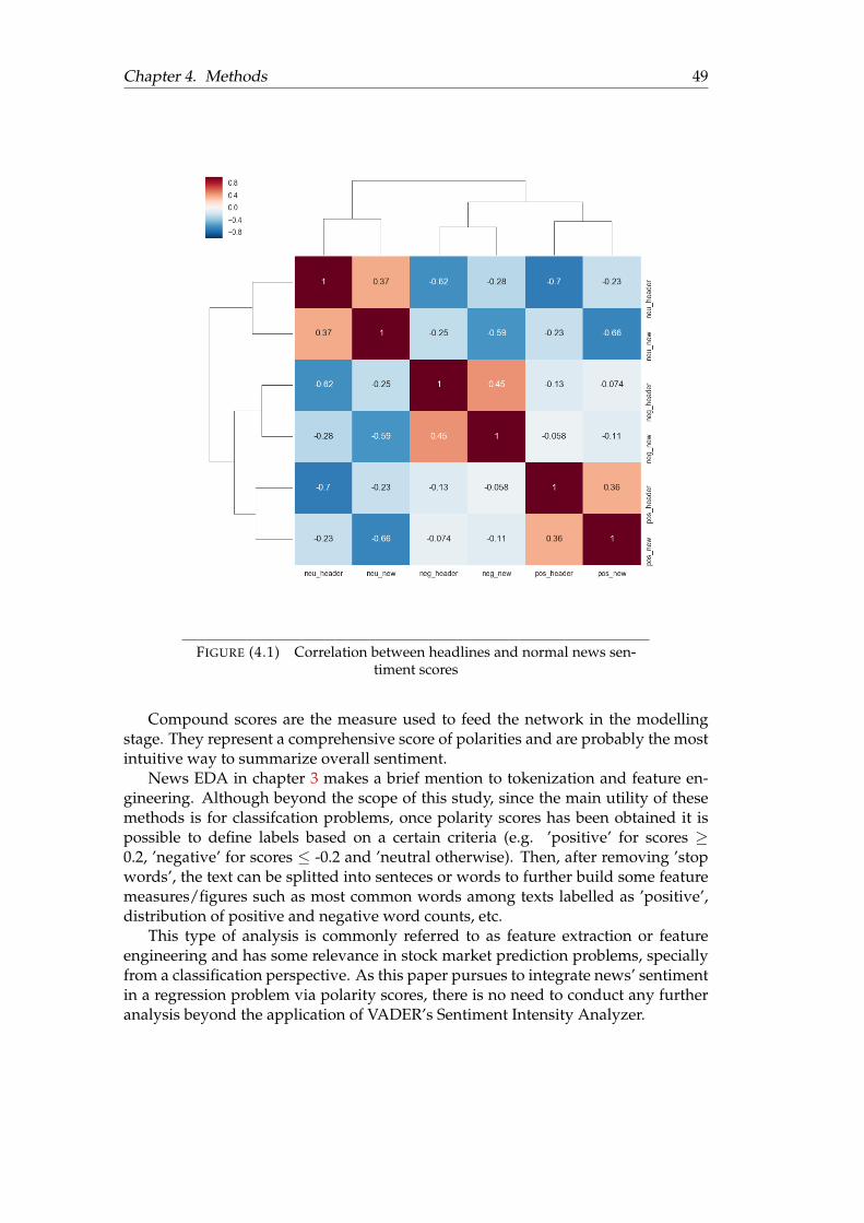
Chapter 4. Methods 49
FIGURE (4.1) Correlation between headlines and normal news sen-timent scores
Compound scores are the measure used to feed the network in the modellingstage. They represent a comprehensive score of polarities and are probably the mostintuitive way to summarize overall sentiment.
News EDA in chapter 3 makes a brief mention to tokenization and feature en-gineering. Although beyond the scope of this study, since the main utility of thesemethods is for classifcation problems, once polarity scores has been obtained it ispossible to define labels based on a certain criteria (e.g. ’positive’ for scores �0.2, ’negative’ for scores -0.2 and ’neutral otherwise). Then, after removing ’stopwords’, the text can be splitted into senteces or words to further build some featuremeasures/figures such as most common words among texts labelled as ’positive’,distribution of positive and negative word counts, etc.
This type of analysis is commonly referred to as feature extraction or featureengineering and has some relevance in stock market prediction problems, speciallyfrom a classification perspective. As this paper pursues to integrate news’ sentimentin a regression problem via polarity scores, there is no need to conduct any furtheranalysis beyond the application of VADER’s Sentiment Intensity Analyzer.
Chapter 4. Methods 50
4.3 LSTM for time series prediction
One of the fundamental problems which plagued traditional feed forward neuralnetworks for a long time since its inception was the ability to identify patterns in se-quence of inputs relying on previous sequences for information and context. From atheoretical point of view, taking into account that neural networks mimic biologicalneurons, it is totally justifiable to include the concept of memory in artificial NN sys-tems since humans do not start their learning process from scratch every second. Forinstance, when reading a text, the meaning of words is based on the understandingof previous words in a sentence which allow for a context to predict what the nextword might be.
Traditional neural networks cannot do this, they take in a stand-alone data vectorof some dimension each time and past information do not persist. A few years ago,this lack of memory seemed a major shortcoming in the learning process since itwas unclear how traditional neural networks could use information about previousevents to predict later ones.
First attemps to tackle this issue used feed forward neural networks with thepeculiarity that the output was fed-back as a new input to provide context on thelast seen events. These architectures are no more than traditional networks withloops inside them, allowing information to persist. As an example 4.11 presents asimple recurrent neural as a length-2 sequence with tanh activations:
yt = f (yt�1, yt�2)
yt = htV + cht = tanh(ht�1W + yt�1U + b)
ht�1 = tanh(ht�2W + yt�2U + b)ht�2 = 0
(4.11)
V is the output of hidden layer t which includes weights W and data units Ufrom t � 1. In fact, RNN are multiple copies of the same network, each one passinga message to subsequent t. While these architectures worked to an extent, the ideathat they are capable of relating previous information to the present event is notalways true. RNN specially suffer from ’long-term’ dependencies, situations wherethe time gap between the present and the past relevant information becomes large5. This represents a major downfall since, in practice, many time series modellingproblems require the information enclosed in past distant data for future predictions.
In theory, RNN are absolutely capable of dealing with such ’long-term depen-dencies’ but the mechanics suffer from the so called vanishing gradient problemwhen trying to learn from distant events. In accordance with the structure definedin ??, a RNN with sequence length x can be ’unrolled’ so that each step back in thepast is added to the model as a new hidden layer. For instance, previous exampleis essentially a two hidden layer network where t considers information exclusivelyfrom the two previous time moments. As more layers are added to the network, tocapture more distant observations, certain activation functions return gradient val-ues close to zero, making the network hard to train. Figure 4.2 depicts an unrolledRNN for some t sequence length being A neural network chunks.
5(Bengio, Simard, and Frasconi, 1994) explores the problem in detail.
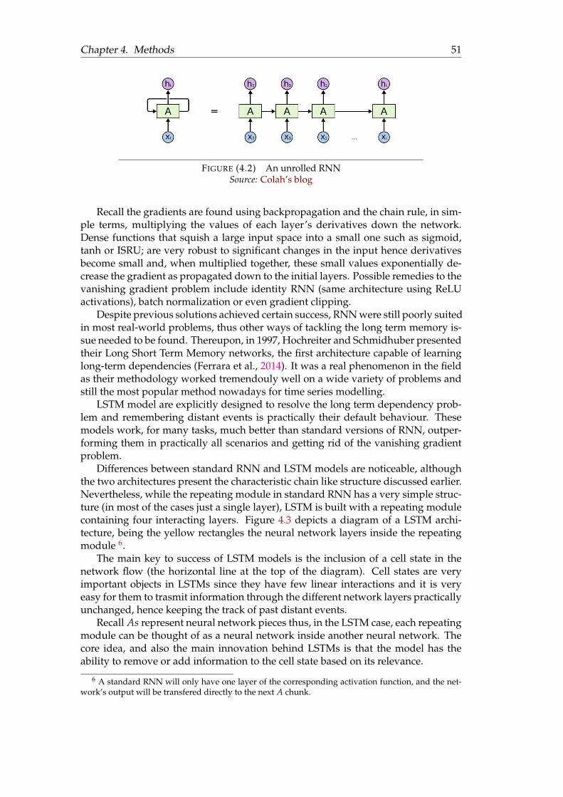
Chapter 4. Methods 51
FIGURE (4.2) An unrolled RNNSource: Colah’s blog
Recall the gradients are found using backpropagation and the chain rule, in sim-ple terms, multiplying the values of each layer’s derivatives down the network.Dense functions that squish a large input space into a small one such as sigmoid,tanh or ISRU; are very robust to significant changes in the input hence derivativesbecome small and, when multiplied together, these small values exponentially de-crease the gradient as propagated down to the initial layers. Possible remedies to thevanishing gradient problem include identity RNN (same architecture using ReLUactivations), batch normalization or even gradient clipping.
Despite previous solutions achieved certain success, RNN were still poorly suitedin most real-world problems, thus other ways of tackling the long term memory is-sue needed to be found. Thereupon, in 1997, Hochreiter and Schmidhuber presentedtheir Long Short Term Memory networks, the first architecture capable of learninglong-term dependencies (Ferrara et al., 2014). It was a real phenomenon in the fieldas their methodology worked tremendouly well on a wide variety of problems andstill the most popular method nowadays for time series modelling.
LSTM model are explicitly designed to resolve the long term dependency prob-lem and remembering distant events is practically their default behaviour. Thesemodels work, for many tasks, much better than standard versions of RNN, outper-forming them in practically all scenarios and getting rid of the vanishing gradientproblem.
Differences between standard RNN and LSTM models are noticeable, althoughthe two architectures present the characteristic chain like structure discussed earlier.Nevertheless, while the repeating module in standard RNN has a very simple struc-ture (in most of the cases just a single layer), LSTM is built with a repeating modulecontaining four interacting layers. Figure 4.3 depicts a diagram of a LSTM archi-tecture, being the yellow rectangles the neural network layers inside the repeatingmodule 6.
The main key to success of LSTM models is the inclusion of a cell state in thenetwork flow (the horizontal line at the top of the diagram). Cell states are veryimportant objects in LSTMs since they have few linear interactions and it is veryeasy for them to trasmit information through the different network layers practicallyunchanged, hence keeping the track of past distant events.
Recall As represent neural network pieces thus, in the LSTM case, each repeatingmodule can be thought of as a neural network inside another neural network. Thecore idea, and also the main innovation behind LSTMs is that the model has theability to remove or add information to the cell state based on its relevance.
6 A standard RNN will only have one layer of the corresponding activation function, and the net-work’s output will be transfered directly to the next A chunk.
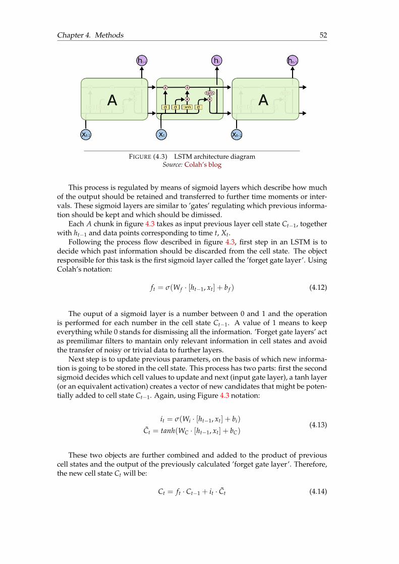
Chapter 4. Methods 52
FIGURE (4.3) LSTM architecture diagramSource: Colah’s blog
This process is regulated by means of sigmoid layers which describe how muchof the output should be retained and transferred to further time moments or inter-vals. These sigmoid layers are similar to ’gates’ regulating which previous informa-tion should be kept and which should be dimissed.
Each A chunk in figure 4.3 takes as input previous layer cell state Ct�1, togetherwith ht�1 and data points corresponding to time t, Xt.
Following the process flow described in figure 4.3, first step in an LSTM is todecide which past information should be discarded from the cell state. The objectresponsible for this task is the first sigmoid layer called the ’forget gate layer’. UsingColah’s notation:
ft = s(Wf · [ht�1, xt] + b f ) (4.12)
The ouput of a sigmoid layer is a number between 0 and 1 and the operationis performed for each number in the cell state Ct�1. A value of 1 means to keepeverything while 0 stands for dismissing all the information. ’Forget gate layers’ actas premilimar filters to mantain only relevant information in cell states and avoidthe transfer of noisy or trivial data to further layers.
Next step is to update previous parameters, on the basis of which new informa-tion is going to be stored in the cell state. This process has two parts: first the secondsigmoid decides which cell values to update and next (input gate layer), a tanh layer(or an equivalent activation) creates a vector of new candidates that might be poten-tially added to cell state Ct�1. Again, using Figure 4.3 notation:
it = s(Wi · [ht�1, xt] + bi)
Ct = tanh(WC · [ht�1, xt] + bC)(4.13)
These two objects are further combined and added to the product of previouscell states and the output of the previously calculated ’forget gate layer’. Therefore,the new cell state Ct will be:
Ct = ft · Ct�1 + it · Ct (4.14)
Chapter 4. Methods 53
The new state is calculated with contributions from previous states and new in-formation of time t, in both cases previously filtered by applying a sigmoid layer tocapture only relevant information.
Finally, last sigmoid layer dedices what to output based on previously calculatedcell state Ct. After applying the sigmoid for filtering purposes, the cell state is passedto a tanh activation (output between -1 and 1) and the result is multiplied by theoutput of the sigmoid gate. Once again, in Colah’s notation:
st = s(Wo · [ht�1, xt] + bo)
ht = st · tanh(Ct)(4.15)
Equation 4.15 is the output of a regular LSTM layer. Previously described ar-chitecture represents a normal LSTM but, although the core idea of the four gatesis essentially the same, the actual placement of the arrows differs depending on theresearch paper allowing for slightly different versions of the model. Differences areminor, mainly related to interactions between the four gates, looking forward to sim-plify the model and adapt it better to the problem treated.
In this paper, the LSTM model employed was originally designed by Jakob Aungiers,2018 and further adapted to include sensitivity scores. As disscussed in the begin-ning of the chapter, the motion of a stock market time series is not any sort of knownfunction, in fact, the best propery to describe them appears to be a random walk. Intheory, a random walk has no predictable patterns hence attempting to model willbe worthless but, fortunately, there are on-going arguments by many experts in thefield arguing that stock price movements are not pure random walks and they havesome sort of hidden pattern.
An important remark is that, as stock prices are constantly moving with no spec-ified boundaries, data normalization is needed, otherwise the model will never con-verge. To combat this, a recommended procedure is to normalize the data by takingpercentage changes from the start of the window hence, in the case of financial timeseries, the output feeded to the network will reflect returns on stock over a rollingwindow of width equal to the specified sequence length. Following equation is usedto normalize the data:
ni =
✓pip0
◆� 1 (4.16)
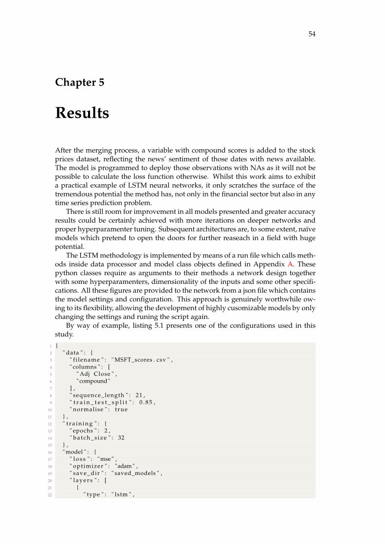
54
Chapter 5
Results
After the merging process, a variable with compound scores is added to the stockprices dataset, reflecting the news’ sentiment of those dates with news available.The model is programmed to deploy those observations with NAs as it will not bepossible to calculate the loss function otherwise. Whilst this work aims to exhibita practical example of LSTM neural networks, it only scratches the surface of thetremendous potential the method has, not only in the financial sector but also in anytime series prediction problem.
There is still room for improvement in all models presented and greater accuracyresults could be certainly achieved with more iterations on deeper networks andproper hyperparamenter tuning. Subsequent architectures are, to some extent, naïvemodels which pretend to open the doors for further reaseach in a field with hugepotential.
The LSTM methodology is implemented by means of a run file which calls meth-ods inside data processor and model class objects defined in Appendix A. Thesepython classes require as arguments to their methods a network design togetherwith some hyperparamenters, dimensionality of the inputs and some other specifi-cations. All these figures are provided to the network from a json file which containsthe model settings and configuration. This approach is genuinely worthwhile ow-ing to its flexibility, allowing the development of highly cusomizable models by onlychanging the settings and runing the script again.
By way of example, listing 5.1 presents one of the configurations used in thisstudy.
1 {2 " data " : {3 " f i lename " : " MSFT_scores . csv " ,4 " columns " : [5 " Adj Close " ,6 "compound"7 ] ,8 " sequence_length " : 21 ,9 " t r a i n _ t e s t _ s p l i t " : 0 . 8 5 ,
10 " normalise " : t rue11 } ,12 " t r a i n i n g " : {13 " epochs " : 2 ,14 " b a t c h _ s i z e " : 3215 } ,16 " model " : {17 " l o s s " : "mse " ,18 " opt imizer " : "adam " ,19 " save_dir " : " saved_models " ,20 " l a y e r s " : [21 {22 " type " : " lstm " ,
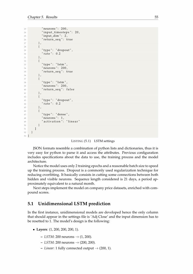
Chapter 5. Results 55
23 " neurons " : 200 ,24 " input_t imesteps " : 20 ,25 " input_dim " : 2 ,26 " re turn_seq " : t rue27 } ,28 {29 " type " : " dropout " ,30 " r a t e " : 0 . 231 } ,32 {33 " type " : " lstm " ,34 " neurons " : 200 ,35 " re turn_seq " : t rue36 } ,37 {38 " type " : " lstm " ,39 " neurons " : 200 ,40 " re turn_seq " : f a l s e41 } ,42 {43 " type " : " dropout " ,44 " r a t e " : 0 . 245 } ,46 {47 " type " : " dense " ,48 " neurons " : 1 ,49 " a c t i v a t i o n " : " l i n e a r "50 }51 ]52 }53 }
LISTING (5.1) LSTM settings
JSON formats resemble a combination of python lists and dictionaries, thus it isvery easy for python to parse it and access the attributes. Previous configurationincludes specifications about the data to use, the training process and the modelarchitecture.
Notice the model uses only 2 training epochs and a reasonable batch size to speedup the training process. Dropout is a commonly used regularization technique forreducing overfitting. It basically consists in cutting some connections between bothhidden and visible neurons. Sequence length considered is 21 days, a period ap-proximately equivalent to a natural month.
Next steps implement the model on company price datasets, enriched with com-pound scores.
5.1 Unidimensional LSTM prediction
In the first instance, unidimensional models are developed hence the only columnthat should appear in the settings file is ’Adj Close’ and the input dimension has tobe resetted to 1. The model’s design is the following:
• Layers: (1, 200, 200, 200, 1).
– LSTM: 200 neurons ! (1, 200).– LSTM: 200 neurons ! (200, 200).– Linear: 1 fully connected output ! (200, 1).
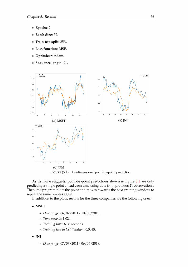
Chapter 5. Results 56
• Epochs: 2.
• Batch Size: 32.
• Train-test split: 85%.
• Loss function: MSE.
• Optimizer: Adam.
• Sequence length: 21.
(A) MSFT (B) JNJ
(C) JPMFIGURE (5.1) Unidimensional point-by-point prediction
As its name suggests, point-by-point predictions shown in figure 5.1 are onlypredicting a single point ahead each time using data from previous 21 observations.Then, the program plots the point and moves towards the next training window torepeat the same process again.
In addition to the plots, results for the three companies are the following ones:
• MSFT
– Date range: 06/07/2011 - 10/06/2019.– Time periods: 1.024.– Training time: 6,98 seconds.– Training loss in last iteration: 0,0015.
• JNJ
– Date range: 07/07/2011 - 06/06/2019.
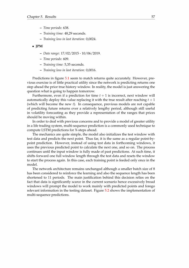
Chapter 5. Results 57
– Time periods: 638.– Training time: 48,29 seconds.– Training loss in last iteration: 0,0024.
• JPM
– Date range: 17/02/2015 - 10/06/2019.– Time periods: 609.– Training time: 5,35 seconds.– Training loss in last iteration: 0,0016.
Predictions in figure 5.1 seem to match returns quite accurately. However, pre-vious exercise is of little practical utility since the network is predicting returns onestep ahead the prior true history window. In reality, the model is just answering thequestion what is going to happen tomorrow.
Furthermore, even if a prediction for time t + 1 is incorrect, next window willautomatically deploy this value replacing it with the true result after reaching t + 1(which will become the new t). In consequence, previous models are not capableof predicting future returns over a relatively lengthy period, although still usefulin volatility forecasting as they provide a representation of the ranges that pricesshould be moving within.
In order to deal with previous concerns and to provide a model of greater utilityin a life trading system, multi-sequence prediction is a commonly used technique tocompute LSTM predictions for X-steps ahead.
The mechanics are quite simple, the model also initializes the test window withtest data and predicts the next point. Thus far, it is the same as a regular point-by-point prediction. However, instead of using test data in forthcoming windows, ituses the previous predicted point to calculate the next one, and so on. The processcontinues until the input window is fully made of past predictions. At such time, itshifts forward one full window length through the test data and resets the windowto start the process again. In this case, each training point is feeded only once in themodel.
The network architecture remains unchanged although a smaller batch size of 8has been considered to reinforce the learning and also the sequence length has beenshortened to 11 periods. The main justification behind this decision relies on thefact that data is significantly scarce in the current scenario hence excessively broadwindows will prompt the model to work mainly with predicted points and foregorelevant information in the testing dataset. Figure 5.2 shows the implementation ofmulti-sequence predictions.
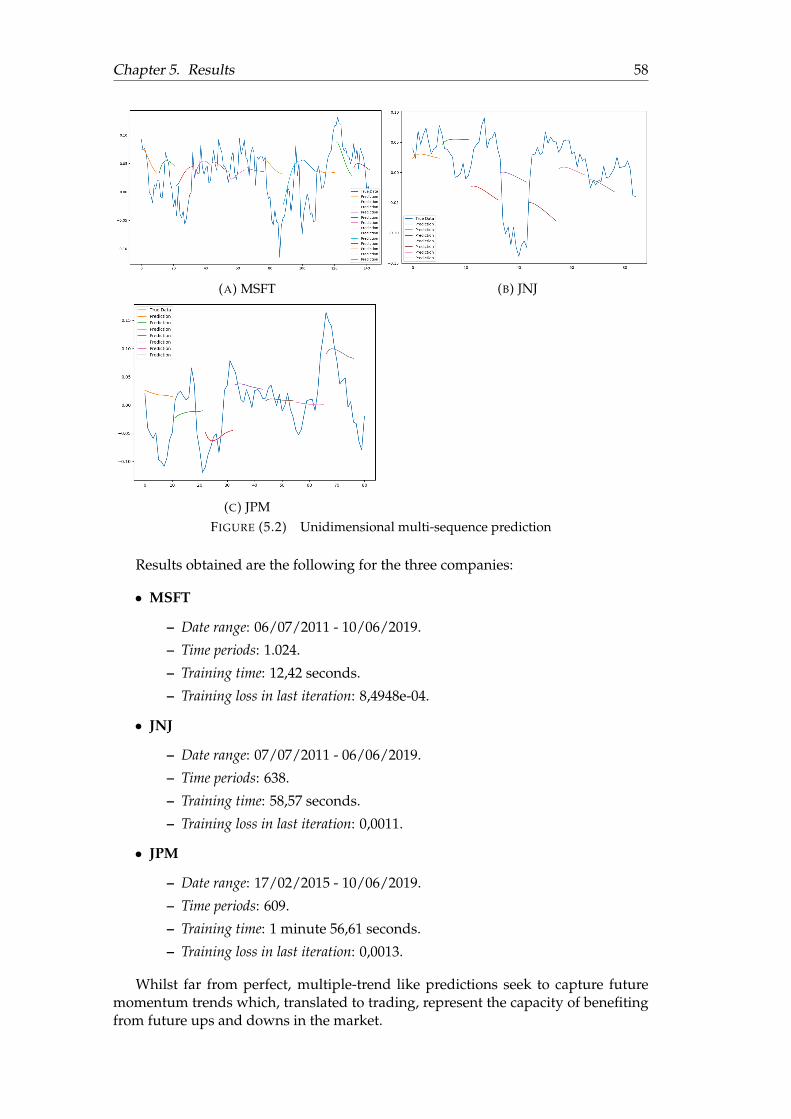
Chapter 5. Results 58
(A) MSFT (B) JNJ
(C) JPMFIGURE (5.2) Unidimensional multi-sequence prediction
Results obtained are the following for the three companies:
• MSFT
– Date range: 06/07/2011 - 10/06/2019.– Time periods: 1.024.– Training time: 12,42 seconds.– Training loss in last iteration: 8,4948e-04.
• JNJ
– Date range: 07/07/2011 - 06/06/2019.– Time periods: 638.– Training time: 58,57 seconds.– Training loss in last iteration: 0,0011.
• JPM
– Date range: 17/02/2015 - 10/06/2019.– Time periods: 609.– Training time: 1 minute 56,61 seconds.– Training loss in last iteration: 0,0013.
Whilst far from perfect, multiple-trend like predictions seek to capture futuremomentum trends which, translated to trading, represent the capacity of benefitingfrom future ups and downs in the market.

Chapter 5. Results 59
5.2 Multidimensional LSTM prediction
Thus far, previous models only consider a single variable in their analysis, concretely’Adj Close’ price. However, in this type of analysis, is is believed that other variablesrelated to price data can enrich the training dataset, ultimately leading to a higherperformance of the model.
Chapter 3 showed that Volume and news’ sentiment are magnitudes certainlycorrelated with adjusted close prices therefore, if VADER polarity scores were tobe accurate estimates of news’ sentiment, both variables will presumably improvepreviously obtained result. Accordingly, these two variables are the ’enriching can-didates’ considered.
In this section, the objective is to determine wheteher Volume or compoundscores are better enriching factors for company price data in terms of model perfor-mance. In line with the argument presented in previous section, multi-sequence pre-dictions are the only ones considered from now on, since point-by-point has provento be of doubtful practical utility in life trading systems.
LSTM class methods in Appendix A are capable of handling multiple dimensionsand, this time, the settings file should be modified in the opposite way as before.Columns should include the two variables considered and the input dimension fieldhas to be assigned a value of 2. Other settings are the same as in the unidimensionalcase.
• Layers: (1, 200, 200, 200, 1).
– LSTM: 200 neurons ! (1, 200).– LSTM: 200 neurons ! (200, 200).– Linear: 1 fully connected output ! (200, 1).
• Epochs: 2.
• Batch Size: 8.
• Train-test split: 85%.
• Loss function: MSE.
• Optimizer: Adam.
• Sequence length: 11.
Predictions using compound scores are displayed in figure 5.3, together with thecorresponding results for each firm:
• MSFT
– Date range: 06/07/2011 - 10/06/2019.– Time periods: 1.024.– Training time: 18,62 seconds.– Training loss in last iteration: 0,0034.
• JNJ
– Date range: 07/07/2011 - 06/06/2019.
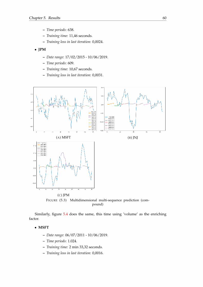
Chapter 5. Results 60
– Time periods: 638.– Training time: 11,46 seconds.– Training loss in last iteration: 0,0024.
• JPM
– Date range: 17/02/2015 - 10/06/2019.– Time periods: 609.– Training time: 10,67 seconds.– Training loss in last iteration: 0,0031.
(A) MSFT (B) JNJ
(C) JPMFIGURE (5.3) Multidimensional multi-sequence prediction (com-
pound)
Similarly, figure 5.4 does the same, this time using ’volume’ as the enrichingfactor.
• MSFT
– Date range: 06/07/2011 - 10/06/2019.– Time periods: 1.024.– Training time: 2 min 33,32 seconds.– Training loss in last iteration: 0,0016.
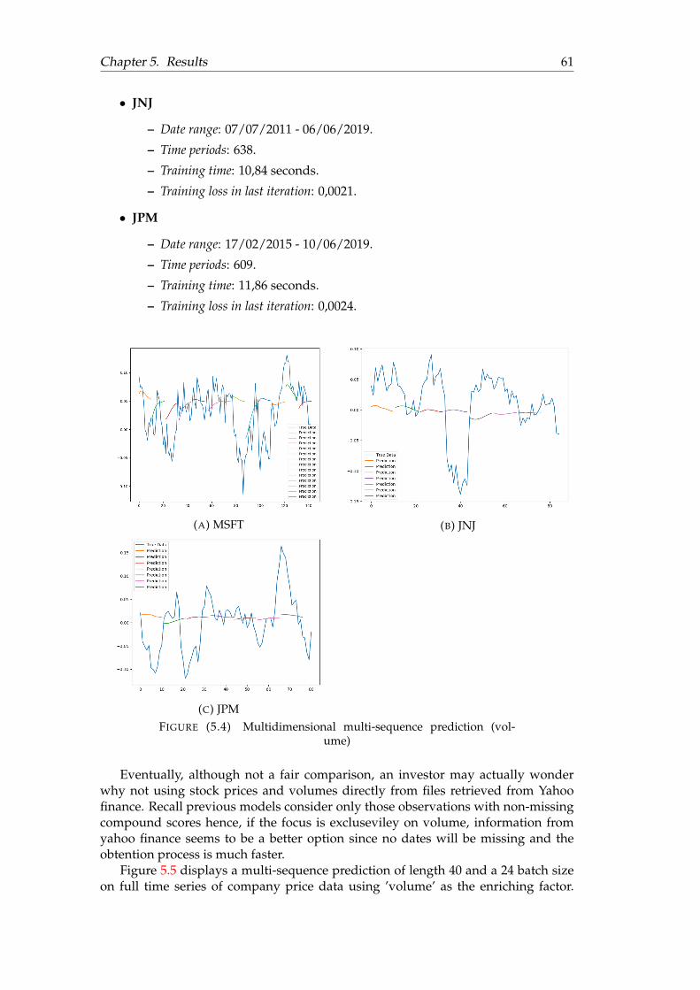
Chapter 5. Results 61
• JNJ
– Date range: 07/07/2011 - 06/06/2019.– Time periods: 638.– Training time: 10,84 seconds.– Training loss in last iteration: 0,0021.
• JPM
– Date range: 17/02/2015 - 10/06/2019.– Time periods: 609.– Training time: 11,86 seconds.– Training loss in last iteration: 0,0024.
(A) MSFT (B) JNJ
(C) JPMFIGURE (5.4) Multidimensional multi-sequence prediction (vol-
ume)
Eventually, although not a fair comparison, an investor may actually wonderwhy not using stock prices and volumes directly from files retrieved from Yahoofinance. Recall previous models consider only those observations with non-missingcompound scores hence, if the focus is excluseviley on volume, information fromyahoo finance seems to be a better option since no dates will be missing and theobtention process is much faster.
Figure 5.5 displays a multi-sequence prediction of length 40 and a 24 batch sizeon full time series of company price data using ’volume’ as the enriching factor.
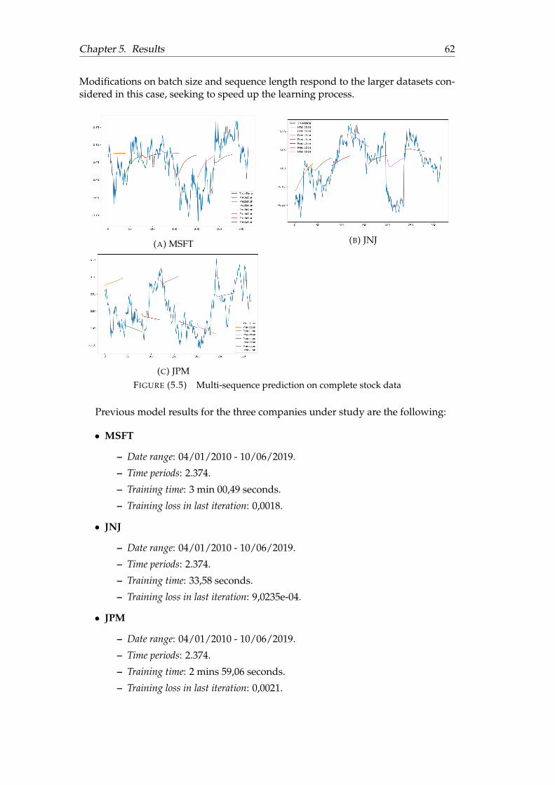
Chapter 5. Results 62
Modifications on batch size and sequence length respond to the larger datasets con-sidered in this case, seeking to speed up the learning process.
(A) MSFT (B) JNJ
(C) JPMFIGURE (5.5) Multi-sequence prediction on complete stock data
Previous model results for the three companies under study are the following:
• MSFT
– Date range: 04/01/2010 - 10/06/2019.– Time periods: 2.374.– Training time: 3 min 00,49 seconds.– Training loss in last iteration: 0,0018.
• JNJ
– Date range: 04/01/2010 - 10/06/2019.– Time periods: 2.374.– Training time: 33,58 seconds.– Training loss in last iteration: 9,0235e-04.
• JPM
– Date range: 04/01/2010 - 10/06/2019.– Time periods: 2.374.– Training time: 2 mins 59,06 seconds.– Training loss in last iteration: 0,0021.
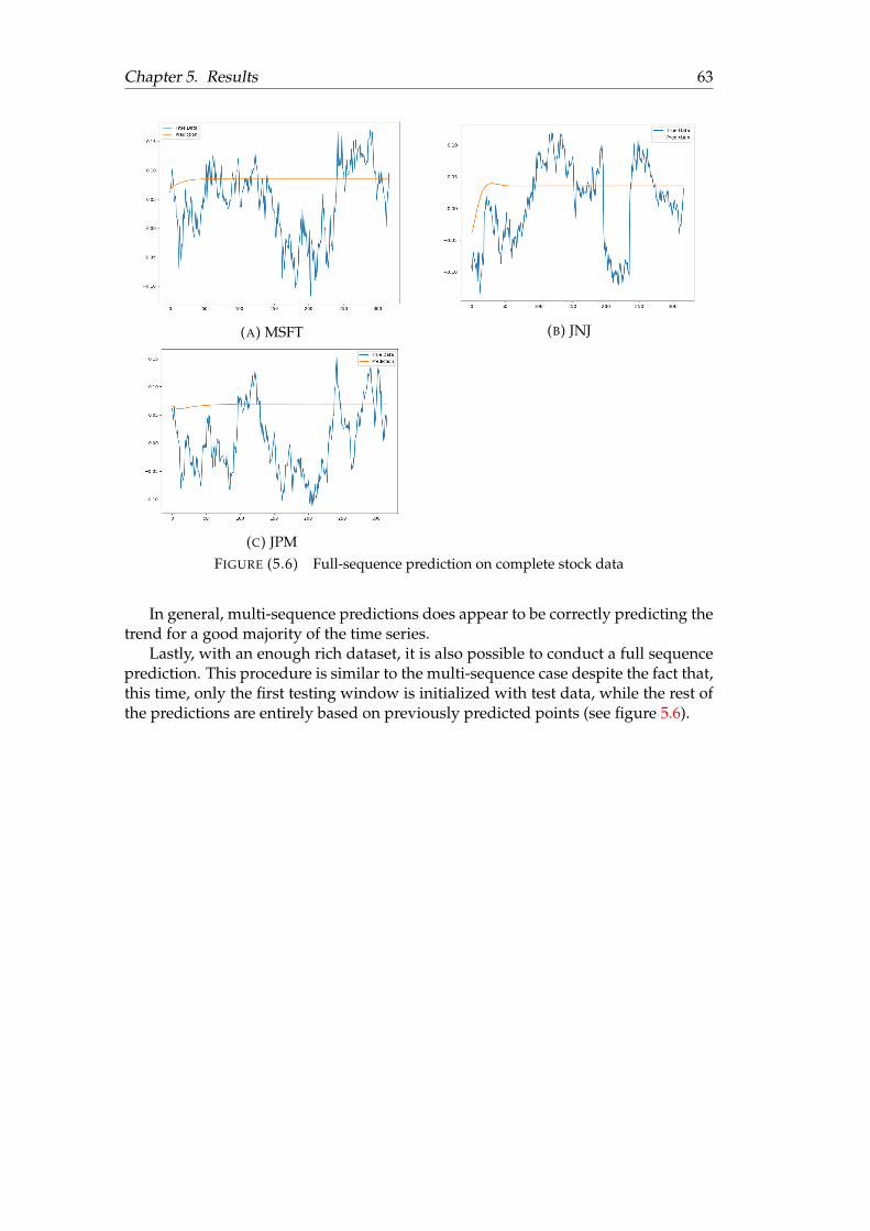
Chapter 5. Results 63
(A) MSFT (B) JNJ
(C) JPMFIGURE (5.6) Full-sequence prediction on complete stock data
In general, multi-sequence predictions does appear to be correctly predicting thetrend for a good majority of the time series.
Lastly, with an enough rich dataset, it is also possible to conduct a full sequenceprediction. This procedure is similar to the multi-sequence case despite the fact that,this time, only the first testing window is initialized with test data, while the rest ofthe predictions are entirely based on previously predicted points (see figure 5.6).
64
Chapter 6
Concluding remarks
Today’s world is being increasingly driven by data. Consumers, companies, publicinstitutions and other agents throughout the globe are constantly generating mas-sive amounts of data. Almost any day-to-day action leaves behind a data trace thatcan be further harvested, preprocessed and analyzed making up the basis of ’BigData’.
Even though ’Big Data’ is a complex issue, if treated appropiately, it can beturned into really valuable insights to inform competitive decision-making and gen-erate value in businesses from a wide range of industries. However, such a boost inthe scale of the information available and steadily generated requires an adaptationof the traditional data science process to more flexible methods capable of living ina highly dynamic environment.
Operational velocity is one of the main issues adressed in this new era, not onlyin data analysis but also througout all stages of the data science process. More pow-erful and sophisticated technologies for data processing are in the market today, thusdata collection techniques should be also aligned with these recent innovations, andweb scraping methods are undoubtedly into the spotlight.
Traditional data collection systems are becoming of less practical utility as timegoes by, being replaced with new mechanisms that essentially ’harvest’ data in-stead of collecting in. With the irruption of Web 2.0, and in today’s world of net-worked and distributed applications, the Internet is becoming the quintessentiallydata source as practically everything is shared through it and, consequently, it con-tains a real universe of information awaiting for a retrieval.
Web scraping tools allow reasearchers and businesses to monitor informationover the net and also an automated data collection on a routinary basis. They alsopermit a highly customizable approach to data extraction in an efficient and fastway, visiting a large number of webpages simultaneously. The vast field of webscraping applications is truly mind-blogging as information on the net is extremelyheterogenous. Competitor price monitoring, market data, financial statements ormovie reviews are just a few examples of data that scrapers can harvest over thenet, to thereafter use them in real-time analytics, as the information can be analyzedright after becoming available.
A web based approach to data extraction processes can definitely improve thequality of our data products. This added value is certainly noticed in the applicationof such methods described in this paper, as financial markets are a clear example ofan scenario where the abovementioned operational velocity is no longer a desire buta necessity.
Either by using an API or by extracting html references from webpages, themethodology employed enables an instantanous disposal of highly heterogenousdata in large quantities. Furthermore, pre-built datsets of the information demanded
Chapter 6. Concluding remarks 65
for this work, with an special emphasis on news data, are either scarce or non-existent, hence web scraping is, in fact, the only plausible alternative to effectivelyretrieve the data needed.
Additionally, a deep learning framework for predictive modelling is also devel-oped, aiming to illustrate a possible use of the already retrieved data in line withpreviously mentioned principles of large data quantities and real-time analysis. Astandard LSTM neural network model is considered in the modelling stage as it hasproven to be a very consistent method for characterizing time series data. The hy-pothesis suggested pretends to test if news data can be a ’enriching factor’ to stockprice predictions, thus improving the accuracy of our models.
Before delving deeper into the details, an important consideration is that all mod-els displayed in chapter 5 can achieve greater accuracy with more training and care-ful hyperparameter tuning. Having said that, figures 5.1a, 5.1b and 5.1c evince themodel is predicting the series very accurately on a point-by-point basis without anyenriching factor. As discussed earlier, although of little relevance in a life tradingsystem, these predictions are still useful in certain applications such as volatilityanalysis or anomaly detection.
As moving towards, in multi-sequence prediction, overfitting is the dominantnote in practically all scenarios, presumably due to data scarcity issues. Traininglosses are small but still the trained network fails to capture certain trends whentested against the ’ground truth’. Overfitting is not resolved by just increasing theepochs in the network, it is a concern which requires further research. A good start,perhaps, is to study the distribution of training losses against test losses.
Besides overfitting issues, if models in figures 5.3 and 5.4 are compared, the in-clusion of polarity scores from news data seems to generate smoother predictionsalthough in many cases, trend estimates are better. On the contrary, enriching priceswith volume makes the model more senstive to abrupt price variations, althoughif lacking them, the model predominantly fails in estimating medium term trendsfor those stocks which are generally more stable. In addition, enriching factors suchas compound polarity scores or volume partially resolve the data scarcity problemsince the network is feeded with more information that can be considered in pre-dictions (compare figures ?? and ?? vs, for instance, figures ?? and ??). In general,although long-term trends seem to be better predicted by including polarity scoresas enrichers instead of volumes, there is not enough evidence to either accept or re-ject the previously stated hypotesis since more data has to be feeded into the modeland, with the available computing resources, the shown data volume is the maxi-mum plausible achievement.
Nevertheless, in terms of practical utility and real applications of the methodol-ogy it is preferrrable to opt for volumes as the data retrieval process is easier, andprediction results achieved when working with complete stock data are certainlysuccesful. In the three cases (figure 5.5c) trend estimates seem to correctly capturefuture data tendencies and, in the case of Johnson & Johnson (figure ??) the model isalso capable of outputting a sensible estimate of the trend over the entire time hori-zon considered. Notice how meaningful is this result since we are saying that given40 days of data entries, the LSTM model can predict a trend for the next 2300 days(approx.) using excusively the previously predicted values as inputs.
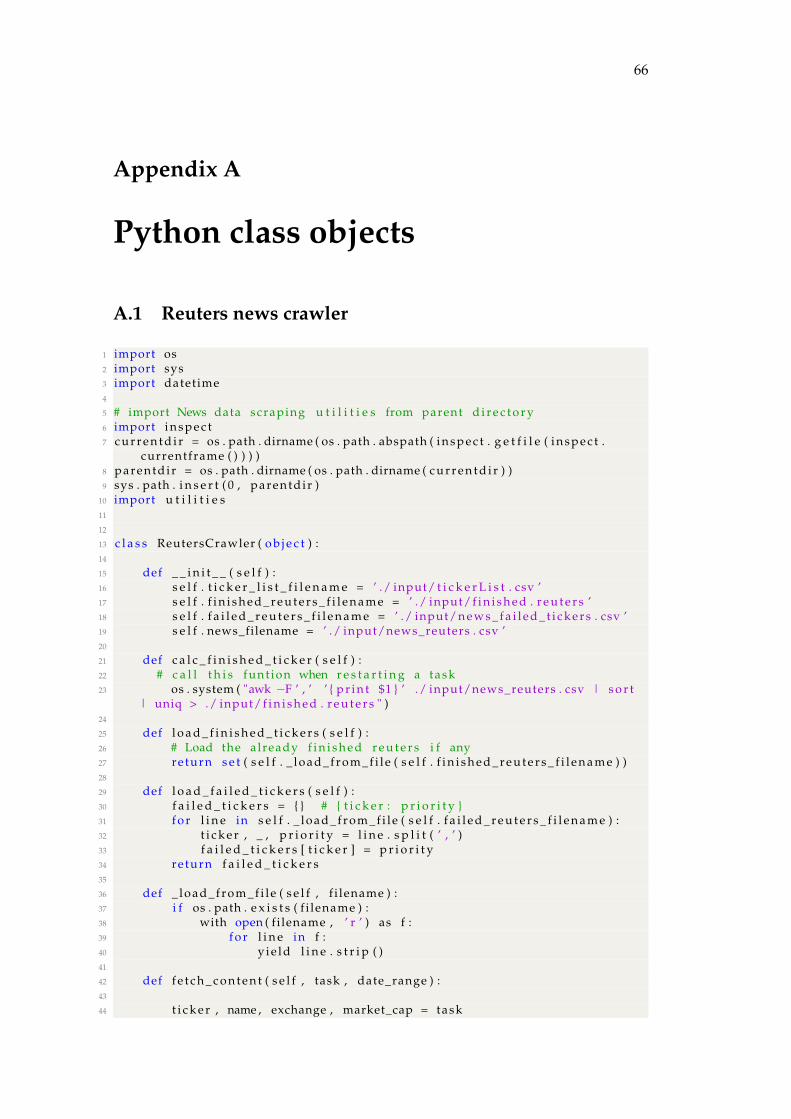
66
Appendix A
Python class objects
A.1 Reuters news crawler
1 import os2 import sys3 import datetime4
5 # import News data scraping u t i l i t i e s from parent d i r e c t o r y6 import i n s p e c t7 c u r r e n t d i r = os . path . dirname ( os . path . abspath ( i n s p e c t . g e t f i l e ( i n s p e c t .
currentframe ( ) ) ) )8 parentd i r = os . path . dirname ( os . path . dirname ( c u r r e n t d i r ) )9 sys . path . i n s e r t ( 0 , parentd i r )
10 import u t i l i t i e s11
12
13 c l a s s ReutersCrawler ( o b j e c t ) :14
15 def _ _ i n i t _ _ ( s e l f ) :16 s e l f . t i c k e r _ l i s t _ f i l e n a m e = ’ ./ input/ t i c k e r L i s t . csv ’17 s e l f . f i n i s h e d _ r e u t e r s _ f i l e n a m e = ’ ./ input/ f i n i s h e d . r e u t e r s ’18 s e l f . f a i l e d _ r e u t e r s _ f i l e n a m e = ’ ./ input/ n e w s _ f a i l e d _ t i c k e r s . csv ’19 s e l f . news_filename = ’ ./ input/news_reuters . csv ’20
21 def c a l c _ f i n i s h e d _ t i c k e r ( s e l f ) :22 # c a l l t h i s funt ion when r e s t a r t i n g a task23 os . system ( "awk �F ’ , ’ ’ { p r i n t $1 } ’ ./ input/news_reuters . csv | s o r t
| uniq > ./ input/ f i n i s h e d . r e u t e r s " )24
25 def l o a d _ f i n i s h e d _ t i c k e r s ( s e l f ) :26 # Load the already f i n i s h e d r e u t e r s i f any27 re turn s e t ( s e l f . _ load_f r om _ f i l e ( s e l f . f i n i s h e d _ r e u t e r s _ f i l e n a m e ) )28
29 def l o a d _ f a i l e d _ t i c k e r s ( s e l f ) :30 f a i l e d _ t i c k e r s = { } # { t i c k e r : p r i o r i t y }31 f o r l i n e in s e l f . _ load_f rom_f i l e ( s e l f . f a i l e d _ r e u t e r s _ f i l e n a m e ) :32 t i c k e r , _ , p r i o r i t y = l i n e . s p l i t ( ’ , ’ )33 f a i l e d _ t i c k e r s [ t i c k e r ] = p r i o r i t y34 re turn f a i l e d _ t i c k e r s35
36 def _ load_f rom _f i l e ( s e l f , f i lename ) :37 i f os . path . e x i s t s ( f i lename ) :38 with open ( fi lename , ’ r ’ ) as f :39 f o r l i n e in f :40 y i e l d l i n e . s t r i p ( )41
42 def f e t c h _ c o n t e n t ( s e l f , task , date_range ) :43
44 t i c k e r , name , exchange , market_cap = task

Appendix A. Python class objects 67
45 p r i n t ( "%s � %s � %s � %s " % ( t i c k e r , name , exchange , market_cap ) )46
47 s u f f i x = { ’AMEX’ : ’ .A ’ , ’NASDAQ’ : ’ .O’ , ’NYSE ’ : ’ .N’ }48 l i n k = " ht tps ://www. r e u t e r s . com/f inance/s t o c k s/company�news/"49 u r l = l i n k + t i c k e r + s u f f i x [ exchange ]50
51 t i c k e r _ f a i l e d = open ( s e l f . f a i l e d _ r e u t e r s _ f i l e n a m e , ’ a+ ’ )52 today = datetime . datetime . today ( ) . s t r f t i m e ( "%Y%m%d" )53
54 news_num = s e l f . get_news_num_whenever ( u r l )55 i f news_num :56 # I f news , f e t c h f o r N consecut ive days in the past57 has_content , no_news_days = s e l f . fe tch_within_date_range (
news_num , url , date_range , task , t i c k e r )58 i f not has_content :59 p r i n t ( ’%s has no content within date range ’ % t i c k e r )60 i f no_news_days :61 p r i n t ( ’ s e t as LOW p r i o r i t y ’ )62 f o r timestamp in no_news_days :63 t i c k e r _ f a i l e d . wri te ( t i c k e r + ’ , ’ + timestamp + ’ , ’ + ’
LOW\n ’ )64 e l s e :65 # The company has no news even with unspec i f i ed date66 # add i t i n t o the lowest p r i o r i t y l i s t67 p r i n t ( "%s has no news at a l l , s e t as LOWEST p r i o r i t y " % (
t i c k e r ) )68 t i c k e r _ f a i l e d . wri te ( t i c k e r + ’ , ’ + today + ’ , ’ + ’LOWEST\n ’ )69 t i c k e r _ f a i l e d . c l o s e ( )70
71 def get_news_num_whenever ( s e l f , u r l ) :72 # check i f the t i c k e r has any news73 # re turn the number of news74 soup = u t i l i t i e s . get_soup_with_repeat ( url , repeat_t imes =4)75 i f soup :76 re turn len ( soup . f i n d _ a l l ( " div " , { ’ c l a s s ’ : [ ’ topStory ’ , ’
f e a t u r e ’ ] } ) )77 re turn 078
79 def fe tch_within_date_range ( s e l f , news_num , url , date_range , task ,t i c k e r ) :
80 # No news f o r X consecut ive days , stop i t e r a t i n g dates81 # Second�lowest p r i o r i t y l i s t82 missing_days = 083 has_content = Fa l se84 no_news_days = [ ]85 f o r timestamp in date_range :86 p r i n t ( ’ t r y i n g ’+timestamp , end= ’\r ’ , f l u s h=True )87 new_time = timestamp [ 4 : ] + timestamp [ : 4 ]88 soup = u t i l i t i e s . get_soup_with_repeat ( u r l + " ? date=" +
new_time )89 i f soup and s e l f . parse_and_save_news ( soup , task , t i c k e r ,
timestamp ) :90 missing_days = 0 # i f get news , r e s e t missing_days as 091 has_content = True92 e l s e :93 missing_days += 194
95 # the more news_num , the longer we can wait96 i f missing_days > news_num ⇤ 5 + 2 0 :97 # no news in X consecut ive days , stop crawling98 p r i n t ( "%s has no news f o r %d days , stop t h i s candidate . . .
" % ( t i c k e r , missing_days ) )99 break
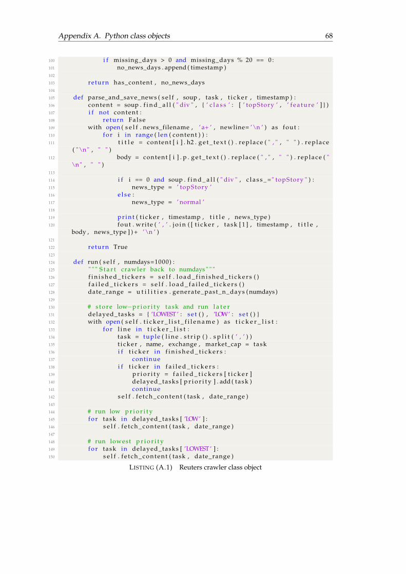
Appendix A. Python class objects 68
100 i f missing_days > 0 and missing_days % 20 == 0 :101 no_news_days . append ( timestamp )102
103 re turn has_content , no_news_days104
105 def parse_and_save_news ( s e l f , soup , task , t i c k e r , timestamp ) :106 content = soup . f i n d _ a l l ( " div " , { ’ c l a s s ’ : [ ’ topStory ’ , ’ f e a t u r e ’ ] } )107 i f not content :108 re turn Fa l se109 with open ( s e l f . news_filename , ’ a+ ’ , newline= ’\n ’ ) as fout :110 f o r i in range ( len ( content ) ) :111 t i t l e = content [ i ] . h2 . g e t _ t e x t ( ) . r e p l a c e ( " , " , " " ) . r e p l a c e
( "\n" , " " )112 body = content [ i ] . p . g e t _ t e x t ( ) . r e p l a c e ( " , " , " " ) . r e p l a c e ( "
\n" , " " )113
114 i f i == 0 and soup . f i n d _ a l l ( " div " , c l a s s _ =" topStory " ) :115 news_type = ’ topStory ’116 e l s e :117 news_type = ’ normal ’118
119 p r i n t ( t i c k e r , timestamp , t i t l e , news_type )120 fout . wri te ( ’ , ’ . j o i n ( [ t i c k e r , task [ 1 ] , timestamp , t i t l e ,
body , news_type ] ) + ’\n ’ )121
122 re turn True123
124 def run ( s e l f , numdays=1000) :125 " " " S t a r t crawler back to numdays " " "126 f i n i s h e d _ t i c k e r s = s e l f . l o a d _ f i n i s h e d _ t i c k e r s ( )127 f a i l e d _ t i c k e r s = s e l f . l o a d _ f a i l e d _ t i c k e r s ( )128 date_range = u t i l i t i e s . generate_past_n_days ( numdays )129
130 # s t o r e low�p r i o r i t y task and run l a t e r131 delayed_tasks = { ’LOWEST ’ : s e t ( ) , ’LOW’ : s e t ( ) }132 with open ( s e l f . t i c k e r _ l i s t _ f i l e n a m e ) as t i c k e r _ l i s t :133 f o r l i n e in t i c k e r _ l i s t :134 task = tuple ( l i n e . s t r i p ( ) . s p l i t ( ’ , ’ ) )135 t i c k e r , name , exchange , market_cap = task136 i f t i c k e r in f i n i s h e d _ t i c k e r s :137 continue138 i f t i c k e r in f a i l e d _ t i c k e r s :139 p r i o r i t y = f a i l e d _ t i c k e r s [ t i c k e r ]140 delayed_tasks [ p r i o r i t y ] . add ( task )141 continue142 s e l f . f e t c h _ c o n t e n t ( task , date_range )143
144 # run low p r i o r i t y145 f o r task in delayed_tasks [ ’LOW’ ] :146 s e l f . f e t c h _ c o n t e n t ( task , date_range )147
148 # run lowest p r i o r i t y149 f o r task in delayed_tasks [ ’LOWEST ’ ] :150 s e l f . f e t c h _ c o n t e n t ( task , date_range )
LISTING (A.1) Reuters crawler class object
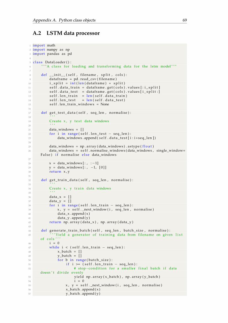
Appendix A. Python class objects 69
A.2 LSTM data processor
1 import math2 import numpy as np3 import pandas as pd4
5 c l a s s DataLoader ( ) :6 " " "A c l a s s f o r loading and transforming data f o r the lstm model " " "7
8 def _ _ i n i t _ _ ( s e l f , f i lename , s p l i t , c o l s ) :9 dataframe = pd . read_csv ( f i lename )
10 i _ s p l i t = i n t ( len ( dataframe ) ⇤ s p l i t )11 s e l f . d a t a _ t r a i n = dataframe . get ( c o l s ) . values [ : i _ s p l i t ]12 s e l f . d a t a _ t e s t = dataframe . get ( c o l s ) . values [ i _ s p l i t : ]13 s e l f . l e n _ t r a i n = len ( s e l f . d a t a _ t r a i n )14 s e l f . l e n _ t e s t = len ( s e l f . d a t a _ t e s t )15 s e l f . len_train_windows = None16
17 def g e t _ t e s t _ d a t a ( s e l f , seq_len , normalise ) :18 ’ ’ ’19 Create x , y t e s t data windows20 ’ ’ ’21 data_windows = [ ]22 f o r i in range ( s e l f . l e n _ t e s t � seq_len ) :23 data_windows . append ( s e l f . d a t a _ t e s t [ i : i +seq_len ] )24
25 data_windows = np . array ( data_windows ) . astype ( f l o a t )26 data_windows = s e l f . normalise_windows ( data_windows , single_window=
False ) i f normalise e l s e data_windows27
28 x = data_windows [ : , :�1]29 y = data_windows [ : , �1, [ 0 ] ]30 re turn x , y31
32 def g e t _ t r a i n _ d a t a ( s e l f , seq_len , normalise ) :33 ’ ’ ’34 Create x , y t r a i n data windows35 ’ ’ ’36 data_x = [ ]37 data_y = [ ]38 f o r i in range ( s e l f . l e n _ t r a i n � seq_len ) :39 x , y = s e l f . _next_window ( i , seq_len , normalise )40 data_x . append ( x )41 data_y . append ( y )42 re turn np . array ( data_x ) , np . array ( data_y )43
44 def g e n e r a t e _ t r a i n _ b a t c h ( s e l f , seq_len , batch_s ize , normalise ) :45 ’ ’ ’ Yie ld a generator of t r a i n i n g data from fi lename on given l i s t
of c o l s ’ ’ ’46 i = 047 while i < ( s e l f . l e n _ t r a i n � seq_len ) :48 x_batch = [ ]49 y_batch = [ ]50 f o r b in range ( b a t c h _ s i z e ) :51 i f i >= ( s e l f . l e n _ t r a i n � seq_len ) :52 # stop�condi t ion f o r a smal ler f i n a l batch i f data
doesn ’ t divide evenly53 y i e l d np . array ( x_batch ) , np . array ( y_batch )54 i = 055 x , y = s e l f . _next_window ( i , seq_len , normalise )56 x_batch . append ( x )57 y_batch . append ( y )
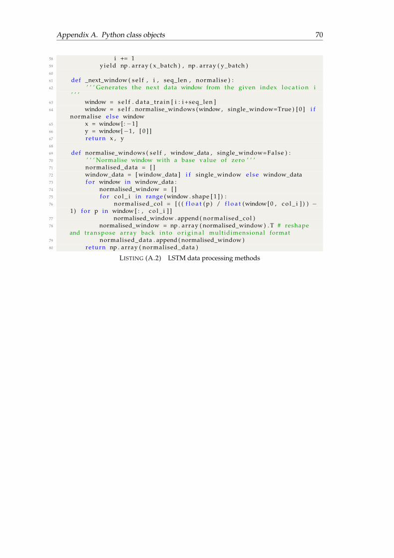
Appendix A. Python class objects 70
58 i += 159 y i e l d np . array ( x_batch ) , np . array ( y_batch )60
61 def _next_window ( s e l f , i , seq_len , normalise ) :62 ’ ’ ’ Generates the next data window from the given index l o c a t i o n i
’ ’ ’63 window = s e l f . d a t a _ t r a i n [ i : i +seq_len ]64 window = s e l f . normalise_windows (window , single_window=True ) [ 0 ] i f
normalise e l s e window65 x = window[: �1]66 y = window[�1 , [ 0 ] ]67 re turn x , y68
69 def normalise_windows ( s e l f , window_data , single_window=Fa l se ) :70 ’ ’ ’ Normalise window with a base value of zero ’ ’ ’71 normalised_data = [ ]72 window_data = [ window_data ] i f single_window e l s e window_data73 f o r window in window_data :74 normalised_window = [ ]75 f o r c o l _ i in range (window . shape [ 1 ] ) :76 normalised_col = [ ( ( f l o a t ( p ) / f l o a t (window [ 0 , c o l _ i ] ) ) �
1) f o r p in window [ : , c o l _ i ] ]77 normalised_window . append ( normalised_col )78 normalised_window = np . array ( normalised_window ) . T # reshape
and transpose array back i n t o o r i g i n a l multidimensional format79 normalised_data . append ( normalised_window )80 re turn np . array ( normalised_data )
LISTING (A.2) LSTM data processing methods
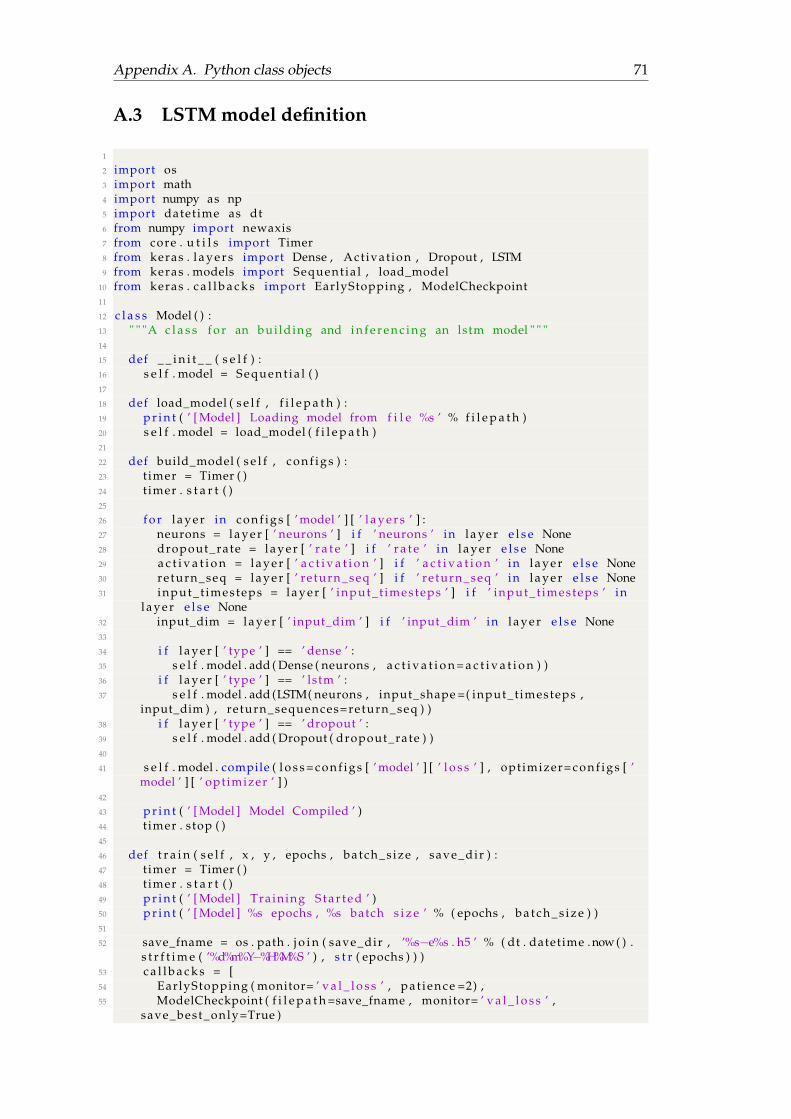
Appendix A. Python class objects 71
A.3 LSTM model definition
1
2 import os3 import math4 import numpy as np5 import datetime as dt6 from numpy import newaxis7 from core . u t i l s import Timer8 from keras . l a y e r s import Dense , Act ivat ion , Dropout , LSTM9 from keras . models import Sequent ia l , load_model
10 from keras . c a l l b a c k s import EarlyStopping , ModelCheckpoint11
12 c l a s s Model ( ) :13 " " "A c l a s s f o r an bui lding and i n f e r e n c i n g an lstm model " " "14
15 def _ _ i n i t _ _ ( s e l f ) :16 s e l f . model = Sequent ia l ( )17
18 def load_model ( s e l f , f i l e p a t h ) :19 p r i n t ( ’ [ Model ] Loading model from f i l e %s ’ % f i l e p a t h )20 s e l f . model = load_model ( f i l e p a t h )21
22 def build_model ( s e l f , c o n f i g s ) :23 t imer = Timer ( )24 t imer . s t a r t ( )25
26 f o r l a y e r in c o n f i g s [ ’ model ’ ] [ ’ l a y e r s ’ ] :27 neurons = l a y e r [ ’ neurons ’ ] i f ’ neurons ’ in l a y e r e l s e None28 dropout_rate = l a y e r [ ’ r a t e ’ ] i f ’ r a t e ’ in l a y e r e l s e None29 a c t i v a t i o n = l a y e r [ ’ a c t i v a t i o n ’ ] i f ’ a c t i v a t i o n ’ in l a y e r e l s e None30 re turn_seq = l a y e r [ ’ re turn_seq ’ ] i f ’ re turn_seq ’ in l a y e r e l s e None31 input_t imesteps = l a y e r [ ’ input_t imesteps ’ ] i f ’ input_t imesteps ’ in
l a y e r e l s e None32 input_dim = l a y e r [ ’ input_dim ’ ] i f ’ input_dim ’ in l a y e r e l s e None33
34 i f l a y e r [ ’ type ’ ] == ’ dense ’ :35 s e l f . model . add ( Dense ( neurons , a c t i v a t i o n = a c t i v a t i o n ) )36 i f l a y e r [ ’ type ’ ] == ’ lstm ’ :37 s e l f . model . add (LSTM( neurons , input_shape =( input_t imesteps ,
input_dim ) , return_sequences=return_seq ) )38 i f l a y e r [ ’ type ’ ] == ’ dropout ’ :39 s e l f . model . add ( Dropout ( dropout_rate ) )40
41 s e l f . model . compile ( l o s s =c o n f i g s [ ’ model ’ ] [ ’ l o s s ’ ] , opt imizer= c o n f i g s [ ’model ’ ] [ ’ opt imizer ’ ] )
42
43 p r i n t ( ’ [ Model ] Model Compiled ’ )44 t imer . stop ( )45
46 def t r a i n ( s e l f , x , y , epochs , batch_s ize , save_dir ) :47 t imer = Timer ( )48 t imer . s t a r t ( )49 p r i n t ( ’ [ Model ] Training S t a r t e d ’ )50 p r i n t ( ’ [ Model ] %s epochs , %s batch s i z e ’ % ( epochs , b a t c h _ s i z e ) )51
52 save_fname = os . path . j o i n ( save_dir , ’%s�e%s . h5 ’ % ( dt . datetime . now ( ) .s t r f t i m e ( ’%d%m%Y�%H%M%S ’ ) , s t r ( epochs ) ) )
53 c a l l b a c k s = [54 EarlyStopping ( monitor= ’ v a l _ l o s s ’ , pa t ience =2) ,55 ModelCheckpoint ( f i l e p a t h =save_fname , monitor= ’ v a l _ l o s s ’ ,
save_best_only=True )
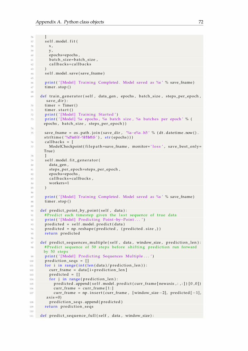
Appendix A. Python class objects 72
56 ]57 s e l f . model . f i t (58 x ,59 y ,60 epochs=epochs ,61 b a t c h _ s i z e=batch_s ize ,62 c a l l b a c k s = c a l l b a c k s63 )64 s e l f . model . save ( save_fname )65
66 p r i n t ( ’ [ Model ] Training Completed . Model saved as %s ’ % save_fname )67 t imer . stop ( )68
69 def t r a i n _ g e n e r a t o r ( s e l f , data_gen , epochs , batch_s ize , steps_per_epoch ,save_dir ) :
70 t imer = Timer ( )71 t imer . s t a r t ( )72 p r i n t ( ’ [ Model ] Training S t a r t e d ’ )73 p r i n t ( ’ [ Model ] %s epochs , %s batch s ize , %s batches per epoch ’ % (
epochs , batch_s ize , steps_per_epoch ) )74
75 save_fname = os . path . j o i n ( save_dir , ’%s�e%s . h5 ’ % ( dt . datetime . now ( ) .s t r f t i m e ( ’%d%m%Y�%H%M%S ’ ) , s t r ( epochs ) ) )
76 c a l l b a c k s = [77 ModelCheckpoint ( f i l e p a t h =save_fname , monitor= ’ l o s s ’ , save_best_only=
True )78 ]79 s e l f . model . f i t _ g e n e r a t o r (80 data_gen ,81 steps_per_epoch=steps_per_epoch ,82 epochs=epochs ,83 c a l l b a c k s =c a l l b a c k s ,84 workers=185 )86
87 p r i n t ( ’ [ Model ] Training Completed . Model saved as %s ’ % save_fname )88 t imer . stop ( )89
90 def predic t_point_by_point ( s e l f , data ) :91 # P r e d i c t each t imestep given the l a s t sequence of t rue data92 p r i n t ( ’ [ Model ] P r e d i c t i n g Point�by�Point . . . ’ )93 predic ted = s e l f . model . p r e d i c t ( data )94 predic ted = np . reshape ( predicted , ( predic ted . s ize , ) )95 re turn predic ted96
97 def predic t_sequences_mul t ip le ( s e l f , data , window_size , p r e d i c t i o n _ l e n ) :98 # P r e d i c t sequence of 50 s teps before s h i f t i n g p r e d i c t i o n run forward
by 50 s teps99 p r i n t ( ’ [ Model ] P r e d i c t i n g Sequences Mult iple . . . ’ )
100 p r e d i c t i o n _ s e q s = [ ]101 f o r i in range ( i n t ( len ( data ) / p r e d i c t i o n _ l e n ) ) :102 curr_frame = data [ i ⇤p r e d i c t i o n _ l e n ]103 predic ted = [ ]104 f o r j in range ( p r e d i c t i o n _ l e n ) :105 predic ted . append ( s e l f . model . p r e d i c t ( curr_frame [ newaxis , : , : ] ) [ 0 , 0 ] )106 curr_frame = curr_frame [ 1 : ]107 curr_frame = np . i n s e r t ( curr_frame , [ window_size �2] , predic ted [ �1] ,
a x i s =0)108 p r e d i c t i o n _ s e q s . append ( predic ted )109 re turn p r e d i c t i o n _ s e q s110
111 def p r e d i c t _ s e q u e n c e _ f u l l ( s e l f , data , window_size ) :
Appendix A. Python class objects 73
112 # S h i f t the window by 1 new p r e d i c t i o n each time , re�run p r e d i c t i o n s onnew window
113 p r i n t ( ’ [ Model ] P r e d i c t i n g Sequences F u l l . . . ’ )114 curr_frame = data [ 0 ]115 predic ted = [ ]116 f o r i in range ( len ( data ) ) :117 predic ted . append ( s e l f . model . p r e d i c t ( curr_frame [ newaxis , : , : ] ) [ 0 , 0 ] )118 curr_frame = curr_frame [ 1 : ]119 curr_frame = np . i n s e r t ( curr_frame , [ window_size �2] , predic ted [ �1] ,
a x i s =0)120 re turn predic ted
LISTING (A.3) LSTM model class object

74
Appendix B
Natural Language Processing
B.1 Stop Words
1 ‘ ‘2 =3 >4 |5 �6 ��7 ;8 :9 !
10 ?11 .12 ’ ’13 ’14 "15 " "16 (17 )18 [19 ]20 @21 $22 ⇤23 ⇤⇤24 \&25 \%26 +27 �28 +129 10�k30 10�q31 1/232 +1�646�223�878033 1�b r a z i l34 1�china35 1�u . s .36 201637 201738 201839 21 s t40 2�u . s .41 3d42 3rd43 4 th44 +9145 a46 ’ a

Appendix B. Natural Language Processing 75
47 ’ a�48 ’ a+49 a .50 A51 ’ aa52 ’ aaa53 ab54 abb55 about56 abu57 a f r i c a58 a f r i c a n59 a f t e r60 ago61 a l62 a l b e r t a63 a l i b a b a64 a l l65 a l l e r g a n66 a l s o67 amazon68 amazon . com69 america70 american71 amsterdam72 an73 and74 angeles75 announce76 another77 anthem78 any79 apol lo80 apple81 apply82 a p r i l83 are84 area85 around86 as87 a/s88 a s i a89 ask90 as t razeneca91 a t92 aug93 aug .94 august95 a u s t r a l i a96 a u s t r a l i a n97 automaker98 aviv99 b
100 ’ b101 ’ b+102 b .103 baidu104 bancorp105 bangalore . newsroom106 bank107 b a r c l a y s108 bb109 ’ bb

Appendix B. Natural Language Processing 76
110 ’ bb�111 ’ bb+112 ’ bbb113 ’ bbb�114 ’ bbb+115 bce116 be117 because118 become119 before120 begin121 b e i j i n g122 b e l l123 b i l l i o n124 b i l l i o n a i r e125 b i l l i t o n126 b lackstone127 bln128 bloomberg129 boeing130 book131 boston132 both133 b r a z i l134 b r a z i l i a n135 b r i e f136 b r i e f�aegon137 b r i e f�american138 b r i e f�taiwan139 b r i t a i n140 b r i t i s h141 b r u s s e l s142 bt143 business144 by145 c146 c .147 ca148 ca lgary149 c a l i f o r n i a150 can151 canada152 canadian153 car154 c a r o l i n a155 case156 cent157 century158 �ceo159 c e r t a i n160 c f161 chase162 chevron163 chicago164 china165 c igna166 c i s c o167 c i t e168 c i t i169 c i t i g r o u p170 cme171 cnbc172 co

Appendix B. Natural Language Processing 77
173 co .174 coca�co la175 colombia176 comcast177 company178 corp179 corp .180 corporate181 corporat ion182 customer183 d .184 dan185 data186 date187 day188 day�189 de190 dec191 dec .192 december193 d e l l194 d e l t a195 d e t r o i t196 deutsche197 disney198 do199 doj200 d o l l a r201 don202 donald203 dow204 dr .205 dubai206 during207 dutch208 e209 e .210 e a s t211 e i g h t212 eikon213 e l214 e l i215 e⇤ t rade216 eu217 euro218 europe219 europe220 european221 event222 exchange223 exxon224 f225 ’ f1226 ’ f2227 f�35228 facebook229 fargo230 f a s t�food231 f / c a s t232 feb233 february234 f e l l235 f f o

Appendix B. Natural Language Processing 78
236 f i e l d237 f i l e238 f i n a l239 f irm240 f i r s t241 f i r s t �quarter242 f i t c h243 f i v e244 f l a .245 f l o r i d a246 f o r247 ford248 four249 fourth250 fourth�quarter251 fox252 f rance253 f r a n c i s c o254 f r a n k f u r t255 f rench256 f r i d a y257 from258 f u l l�year259 f u r t h e r260 fy261 fy2016262 g263 gaap264 ge265 george266 germany267 get268 give269 g laxosmithkl ine270 gm271 gmt272 goldman273 google274 gopro275 gp276 green277 group278 h279 h1280 ha281 h a l t282 has283 have284 hbo285 he286 h i s287 holiday288 home289 honda290 houston291 how292 hsbc293 ht tp294 humana295 i296 i /b/e/s297 ibm298 icahn

Appendix B. Natural Language Processing 79
299 i c i c i300 i d r301 i f302 i f r303 i i304 immuno�oncology305 in306 inbev307 inc308 inc .309 index310 india311 indian312 indonesia313 i n t e r n a t i o n a l314 i n t o315 iphone316 i s317 i s r a e l i318 i t319 i t a l i a320 item321 i t s322 iv323 j324 j .325 j an .326 january327 japan328 japanese329 j . c .330 j e f f r e y331 job332 john333 johnson334 j o u r n a l335 jp336 j . p .337 jpmorgan338 j r .339 j u l y340 june341 j u s t342 j v343 k344 ke l logg345 kfc346 korea347 l348 l .349 l�3350 l e351 l e t352 l e t t e r353 lg354 l i k e l y355 l i n k356 l l c357 lng358 l o c a l359 l o c a l /gmt360 lockheed361 london

Appendix B. Natural Language Processing 80
362 look363 lp364 l . p365 l . p .366 l t d367 l t d .368 lynch369 m370 m.371 main372 make373 march374 market375 may376 mcdonald377 m e r r i l l378 mexico379 michael380 microsof t381 m i l l i o n382 mln383 mobil384 monday385 monsanto386 moody387 morgan388 mt389 must390 m/v391 mylan392 name393 nasdaq394 near395 n e t f l i x396 next397 nike398 n ikke i399 nine400 no . 2401 nokia402 non�t imely403 nordisk404 norm405 north406 northern407 norwegian408 note409 nov410 nov .411 novo412 now413 nv414 nyse415 o416 obama417 oc t418 october419 of420 o i421 on422 one423 or424 other
Appendix B. Natural Language Processing 81
425 our426 over427 p428 p .429 pa430 parent431 par t432 par tner433 past434 paulo435 pc436 pct437 pdvsa438 per439 percent440 period441 petrobras442 p f i z e r443 phase444 place445 p lc446 point447 poland448 previously449 q1450 q2451 q3452 q4453 q t r l y454 quar ter455 q u a r t e r l y456 r457 r .458 ralph459 r e c e n t460 r e c e n t l y461 region462 r e l a t e463 repor t464 r e p o r t s465 r e s u l t466 r e u t e r s467 r i chard468 r i c o469 r i g470 r i o471 russ ian472 s473 ’ s474 s .475 sa476 s . a .477 san478 sanc t ion479 sao480 saturday481 say482 says483 se484 season485 s e a t t l e486 sec487 �sec
Appendix B. Natural Language Processing 82
488 second489 second�quarter490 s e c t o r491 sedan492 sept493 sept .494 september495 s e r i e s496 s e r v i c e497 s e t498 shanghai499 she500 shr501 s ingapore502 s i x503 s i x t h504 s i z e505 sk506 so507 so�c a l l e d508 some509 son510 sony511 soon512 �sources513 south514 southern515 spor t516 squibb517 s t518 s t .519 s t a n l e y520 s t a r t�up521 s t a t e522 s t i l l523 s tocks�t s x524 s tocks�wall525 s t r u g g l e526 such527 s u i s s e528 sunday529 sweeten530 swiss531 sydney532 t533 t .534 taiwan535 take536 tap537 td538 t e l539 telecom540 t e l e f o n i c a541 t e l l542 ten543 t e s l a544 teva545 t h a i546 than547 t h a t548 the549 t h e i r550 them

Appendix B. Natural Language Processing 83
551 there552 they553 t h i r d554 th ird�quarter555 t h i s556 thomson557 thomsonreuters . com558 those559 through560 thursday561 t�mobile562 to563 tokyo564 too565 toronto566 t o t a l567 toyota568 transcanada569 tuesday570 tv571 t w i t t e r572 two573 type574 u575 ubs576 uk577 uni t578 us579 u . s580 u . s .581 usa582 u . s .�based583 user584 u . s .� l i s t e d585 u t i l i t y586 v587 verizon588 vers ion589 versus590 viacom591 v i sa592 volkswagen593 volume594 vs .595 w596 w.597 wa598 wall599 wal�mart600 walt601 warner602 was603 washington604 we605 web606 website607 wednesday608 week609 wel ls610 were611 west612 what613 when

Appendix B. Natural Language Processing 84
614 where615 whether616 which617 who618 whose619 w i l l620 wi l l iams621 with622 within623 wo624 world625 would626 wsj627 x628 x l629 year630 year�ago631 yet632 york633 you634 y/y635 zuckerberg
LISTING (B.1) Stop Words
B.2 Punctuation List
1 PUNC_LIST = [2 " . " ,3 " ! " ,4 " ? " ,5 " , " ,6 " ; " ,7 " : " ,8 "�" ,9 " ’ " ,
10 " \ " " ,11 " ! ! " ,12 " ! ! ! " ,13 " ? ? " ,14 " ? ? ? " ,15 " ? ! ? " ,16 " ! ? ! " ,17 " ? ! ? ! " ,18 " ! ? ! ? " ,19 ]
LISTING (B.2) VADER punctuation list
B.3 Negate List
1 NEGATE = {2 " a i n t " ,3 " arent " ,4 " cannot " ,5 " cant " ,6 " couldnt " ,7 " darent " ,8 " didnt " ,9 " doesnt " ,
10 " ain ’ t " ,11 " aren ’ t " ,

Appendix B. Natural Language Processing 85
12 " can ’ t " ,13 " couldn ’ t " ,14 " daren ’ t " ,15 " didn ’ t " ,16 " doesn ’ t " ,17 " dont " ,18 " hadnt " ,19 " hasnt " ,20 " havent " ,21 " i s n t " ,22 " mightnt " ,23 " mustnt " ,24 " n e i t h e r " ,25 " don ’ t " ,26 " hadn ’ t " ,27 " hasn ’ t " ,28 " haven ’ t " ,29 " isn ’ t " ,30 " mightn ’ t " ,31 " mustn ’ t " ,32 " neednt " ,33 " needn ’ t " ,34 " never " ,35 " none " ,36 " nope " ,37 " nor " ,38 " not " ,39 " nothing " ,40 " nowhere " ,41 " oughtnt " ,42 " shant " ,43 " shouldnt " ,44 "uhuh " ,45 " wasnt " ,46 " werent " ,47 " oughtn ’ t " ,48 " shan ’ t " ,49 " shouldn ’ t " ,50 "uh�uh " ,51 "wasn ’ t " ,52 " weren ’ t " ,53 " without " ,54 " wont " ,55 " wouldnt " ,56 "won’ t " ,57 " wouldn ’ t " ,58 " r a r e l y " ,59 " seldom " ,60 " desp i te " ,61 }
LISTING (B.3) VADER negate list
B.4 Booster Dictionary
1 BOOSTER_DICT = {2 " a b s o l u t e l y " : B_INCR ,3 " amazingly " : B_INCR ,4 " awfully " : B_INCR ,5 " completely " : B_INCR ,6 " cons iderably " : B_INCR ,7 " decidedly " : B_INCR ,

Appendix B. Natural Language Processing 86
8 " deeply " : B_INCR ,9 " e f f i n g " : B_INCR ,
10 " enormously " : B_INCR ,11 " e n t i r e l y " : B_INCR ,12 " e s p e c i a l l y " : B_INCR ,13 " e x c e p t i o n a l l y " : B_INCR ,14 " extremely " : B_INCR ,15 " fabulous ly " : B_INCR ,16 " f l i p p i n g " : B_INCR ,17 " f l i p p i n " : B_INCR ,18 " f r i c k i n g " : B_INCR ,19 " f r i c k i n " : B_INCR ,20 " f r i g g i n g " : B_INCR ,21 " f r i g g i n " : B_INCR ,22 " f u l l y " : B_INCR ,23 " fucking " : B_INCR ,24 " g r e a t l y " : B_INCR ,25 " h e l l a " : B_INCR ,26 " highly " : B_INCR ,27 " hugely " : B_INCR ,28 " i n c r e d i b l y " : B_INCR ,29 " i n t e n s e l y " : B_INCR ,30 " majorly " : B_INCR ,31 " more " : B_INCR ,32 " most " : B_INCR ,33 " p a r t i c u l a r l y " : B_INCR ,34 " purely " : B_INCR ,35 " qu i te " : B_INCR ,36 " r e a l l y " : B_INCR ,37 " remarkably " : B_INCR ,38 " so " : B_INCR ,39 " s u b s t a n t i a l l y " : B_INCR ,40 " thoroughly " : B_INCR ,41 " t o t a l l y " : B_INCR ,42 " tremendously " : B_INCR ,43 " uber " : B_INCR ,44 " unbel ievably " : B_INCR ,45 " unusually " : B_INCR ,46 " u t t e r l y " : B_INCR ,47 " very " : B_INCR ,48 " almost " : B_DECR,49 " bare ly " : B_DECR,50 " hardly " : B_DECR,51 " j u s t enough " : B_DECR,52 " kind of " : B_DECR,53 " kinda " : B_DECR,54 " kindof " : B_DECR,55 " kind�of " : B_DECR,56 " l e s s " : B_DECR,57 " l i t t l e " : B_DECR,58 " marginal ly " : B_DECR,59 " o c c a s i o n a l l y " : B_DECR,60 " p a r t l y " : B_DECR,61 " s c a r c e l y " : B_DECR,62 " s l i g h t l y " : B_DECR,63 " somewhat " : B_DECR,64 " s o r t of " : B_DECR,65 " s o r t a " : B_DECR,66 " s o r t o f " : B_DECR,67 " sor t�of " : B_DECR,68 }
LISTING (B.4) VADER booster dictionary

Appendix B. Natural Language Processing 87
B.5 Special case idioms
1 SPECIAL_CASE_IDIOMS = {2 " the s h i t " : 3 ,3 " the bomb " : 3 ,4 " bad ass " : 1 . 5 ,5 " yeah r i g h t " : �2,6 " cut the mustard " : 2 ,7 " k i s s of death " : �1.5 ,8 " hand to mouth " : �2,9 }
LISTING (B.5) VADER special case idioms

88
Bibliography
Aggarwal, Charu C (2014). Data classification: algorithms and applications. CRC press.
Arlot, Sylvain, Alain Celisse, et al. (2010). “A survey of cross-validation proceduresfor model selection”. In: Statistics surveys 4, pp. 40–79.
Bengio, Yoshua, Patrice Simard, Paolo Frasconi, et al. (1994). “Learning long-termdependencies with gradient descent is difficult”. In: IEEE transactions on neuralnetworks 5.2, pp. 157–166.
Berners-Lee, Tim, James Hendler, Ora Lassila, et al. (2001). “The semantic web”. In:Scientific american 284.5, pp. 28–37.
Boeing, Geoff and Paul Waddell (2017). “New insights into rental housing marketsacross the united states: web scraping and analyzing craigslist rental listings”.In: Journal of Planning Education and Research 37.4, pp. 457–476.
Chaulagain, Ram et al. (2017). “Cloud Based Web Scraping for Big Data Applica-tions”. In: pp. 138–143. DOI: 10.1109/SmartCloud.2017.28.
Cox, M. and D. Ellsworth (1997). “Application-controlled demand paging for out-of-core visualization”. In: pp. 235–244. DOI: 10.1109/VISUAL.1997.663888.
Crane, DJ (1997). “How the Web is changing the business of business information.”In: Electronic Library 15.4, pp. 311 –316. ISSN: 0264-0473. URL: https : / / www .emeraldinsight.com/doi/abs/10.1108/eb045575.
Cybenko, George (1989). “Approximations by superpositions of a sigmoidal func-tion”. In: Mathematics of Control, Signals and Systems 2, pp. 183–192.
Denning, PJ (1990). “Saving all the bits”. In: American Scientist 78.5, pp. 402 –405.ISSN: 00030996. URL: https://ntrs.nasa.gov/search.jsp?R=19910023503.
Ferrara, Emilio et al. (2014). “Web data extraction, applications and techniques: Asurvey”. In: Knowledge-based systems 70, pp. 301–323.
Hackeling, Gavin (2017). Mastering Machine Learning with scikit-learn. Packt Publish-ing Ltd.
Hanin, Boris (2017). “Universal function approximation by deep neural nets withbounded width and relu activations”. In: arXiv preprint arXiv:1708.02691.
Hawkins, Douglas M (2004). “The problem of overfitting”. In: Journal of chemical in-formation and computer sciences 44.1, pp. 1–12.
Hutto, Clayton J and Eric Gilbert (2014). “Vader: A parsimonious rule-based modelfor sentiment analysis of social media text”. In: Eighth international AAAI confer-ence on weblogs and social media.
Johnston, Alan B and Daniel C Burnett (2012). WebRTC: APIs and RTCWEB protocolsof the HTML5 real-time web. Digital Codex LLC.

BIBLIOGRAPHY 89
Jothimani, Dhanya, Ravi Shankar, and Surendra S Yadav (2018). “A big data analyt-ical framework for portfolio optimization”. In: arXiv preprint arXiv:1811.07188.
Karlik, Bekir and A Vehbi Olgac (2011). “Performance analysis of various activationfunctions in generalized MLP architectures of neural networks”. In: InternationalJournal of Artificial Intelligence and Expert Systems 1.4, pp. 111–122.
Kirkpatrick II, Charles D and Julie A Dahlquist (2010). Technical analysis: the completeresource for financial market technicians. FT press.
Kleene, Stephen C (1956). “Automata studies”. In:
Krotov, Vlad and Matthew Tennyson (2018a). “Tutorial: Web Scraping in the R Lan-guage”. In:
— (2018b). “Tutorial: Web Scraping in the R Language”. In:
Laney, Doug (2001). “3D data management: Controlling data volume, velocity andvariety”. In: META group research note 6.70, p. 1.
Lantz, Brett (2015). Machine learning with R. Packt Publishing Ltd.
Lawson, Richard (2015). Web scraping with Python. Packt Publishing Ltd.
LeCun, Yann, Yoshua Bengio, and Geoffrey Hinton (2015). “Deep learning”. In: na-ture 521.7553, p. 436.
Lesk, Michael (1997). “Digital Libraries: A Unifying or Distributing Force?.” In: URL:https://eric.ed.gov/?id=ED414929.
McCulloch, Warren S and Walter Pitts (1943). “A logical calculus of the ideas imma-nent in nervous activity”. In: The bulletin of mathematical biophysics 5.4, pp. 115–133.
Michael, Katina and Keith W Miller (2013). “Big data: New opportunities and newchallenges [guest editors’ introduction]”. In: Computer 46.6, pp. 22–24.
Saldaña, Zoe Wilkinson (2018). “Sentiment Analysis for Exploratory Data Analy-sis”. In: URL: https://programminghistorian.org/en/lessons/sentiment-analysis.
Shah, Vatsal H (2007). “Machine learning techniques for stock prediction”. In: Foun-dations of Machine Learning| Spring 1.1, pp. 6–12.
Trifunovic, Nemanja et al. (2015). “Paradigm Shift in Big Data SuperComputing:DataFlow vs. ControlFlow”. In: Journal of Big Data 2.1, p. 4. ISSN: 2196-1115. DOI:10.1186/s40537-014-0010-z. URL: https://doi.org/10.1186/s40537-014-0010-z.
Zhu, Xiaojin and Andrew B Goldberg (2009). “Introduction to semi-supervised learn-ing”. In: Synthesis lectures on artificial intelligence and machine learning 3.1, pp. 1–130.
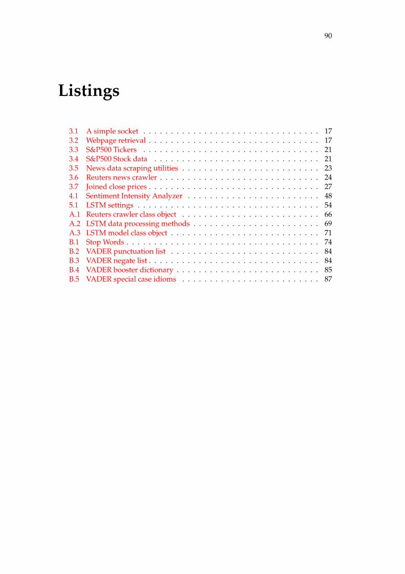
90
Listings
3.1 A simple socket . . . . . . . . . . . . . . . . . . . . . . . . . . . . . . . . 173.2 Webpage retrieval . . . . . . . . . . . . . . . . . . . . . . . . . . . . . . . 173.3 S&P500 Tickers . . . . . . . . . . . . . . . . . . . . . . . . . . . . . . . . 213.4 S&P500 Stock data . . . . . . . . . . . . . . . . . . . . . . . . . . . . . . 213.5 News data scraping utilities . . . . . . . . . . . . . . . . . . . . . . . . . 233.6 Reuters news crawler . . . . . . . . . . . . . . . . . . . . . . . . . . . . . 243.7 Joined close prices . . . . . . . . . . . . . . . . . . . . . . . . . . . . . . . 274.1 Sentiment Intensity Analyzer . . . . . . . . . . . . . . . . . . . . . . . . 485.1 LSTM settings . . . . . . . . . . . . . . . . . . . . . . . . . . . . . . . . . 54A.1 Reuters crawler class object . . . . . . . . . . . . . . . . . . . . . . . . . 66A.2 LSTM data processing methods . . . . . . . . . . . . . . . . . . . . . . . 69A.3 LSTM model class object . . . . . . . . . . . . . . . . . . . . . . . . . . . 71B.1 Stop Words . . . . . . . . . . . . . . . . . . . . . . . . . . . . . . . . . . . 74B.2 VADER punctuation list . . . . . . . . . . . . . . . . . . . . . . . . . . . 84B.3 VADER negate list . . . . . . . . . . . . . . . . . . . . . . . . . . . . . . . 84B.4 VADER booster dictionary . . . . . . . . . . . . . . . . . . . . . . . . . . 85B.5 VADER special case idioms . . . . . . . . . . . . . . . . . . . . . . . . . 87