Embed Size (px)
Citation preview
DEGREE SEQUENCES OF GEOMETRIC PREFERENTIAL ATTACHMENT GRAPHSAuthor(s): JONATHAN JORDANSource: Advances in Applied Probability, Vol. 42, No. 2 (JUNE 2010), pp. 319-330Published by: Applied Probability TrustStable URL: http://www.jstor.org/stable/25683821 .
Accessed: 20/06/2014 07:48
Your use of the JSTOR archive indicates your acceptance of the Terms & Conditions of Use, available at .http://www.jstor.org/page/info/about/policies/terms.jsp
.JSTOR is a not-for-profit service that helps scholars, researchers, and students discover, use, and build upon a wide range ofcontent in a trusted digital archive. We use information technology and tools to increase productivity and facilitate new formsof scholarship. For more information about JSTOR, please contact [email protected].
.
Applied Probability Trust is collaborating with JSTOR to digitize, preserve and extend access to Advances inApplied Probability.
http://www.jstor.org
This content downloaded from 195.34.79.82 on Fri, 20 Jun 2014 07:48:02 AMAll use subject to JSTOR Terms and Conditions
Adv. Appl. Prob. (SGSA) 42, 319-330 (2010) Printed in Northern Ireland
? Applied Probability Trust 2010
DEGREE SEQUENCES OF GEOMETRIC PREFERENTIAL ATTACHMENT GRAPHS
JONATHAN JORDAN,* University of Sheffield
Abstract
We investigate the degree sequence of the geometric preferential attachment model of
Flaxman, Frieze and Vera (2006), (2007) in the case where the self-loop parameter a is set
to 0. We show that, given certain conditions on the attractiveness function F, the degree
sequence converges to the same sequence as found for standard preferential attachment
in Bollobas et al. (2001). We also apply our method to the extended model introduced in van der Esker (2008) which allows for an initial attractiveness term, proving similar
results.
Keywords: Geometric random graph; preferential attachment
2010 Mathematics Subject Classification: Primary 05C80
Secondary 60D05
1. Introduction
In [7] and [8], Flaxman et al. introduced a model for a growing graph driven by geometric
preferential attachment. In this model, which is a variant of the Barabasi-Albert preferential attachment model introduced in [1] and analysed in [3] and [4], vertices are given a random
location in space (similarly to the random geometric graphs of [12] and the SERN model of [2]) and the probability that a new vertex is connected to an already existing vertex u depends on
the distance between them in space as well as on the degree of u.
In this paper we consider a model similar to that of [8] and show that, under certain conditions on the underlying space, the probability measure determining the locations of the vertices, and the strength of the effect of distance on the connection probabilities, the degree distribution
of the graphs produced by our model converges to the same degree distribution as for the
Barabasi-Albert model, first shown rigorously in [4].
1.1. Our model
In this paper we will work with the following model, which is based on that studied in [8]. We assume that S is a compact metric space with metric p and probability measure /x such
that, for any fixed r, ii(Br(x)) is constant as a function of x, where Br(x) is the open p-ball of radius r centred on x. This condition on /x, which is what appears to be necessary for our
proof method, includes the case where S is a sphere and /x is a uniform measure on 5, which was the case considered in [8]; more generally, it includes the case of the Haar measure on a
compact group with an invariant metric. The locations of the added vertices will be assumed to be independent random variables with law /x, and we write Xn for the location of vertex n.
Let F: M+ R+ be an attractiveness function. We will assume that F is continuous, but we allow F(r) ?> oo as r -> 0. Let m e N be the number of vertices that each new vertex will
Received 8 April 2009; revision received 2 February 2010. * Postal address: Department of Probability and Statistics, University of Sheffield, Hicks Building, Sheffield S3 7RH, UK. Email address: [email protected]
319
This content downloaded from 195.34.79.82 on Fri, 20 Jun 2014 07:48:02 AMAll use subject to JSTOR Terms and Conditions
320 SGSA J.JORDAN
be connected to when it is added to the graph. As well as combining the preferential attachment rule with a geometric element, we will also allow a version of the model in which vertices have an initial attractiveness q e (?ra, oo) that modifies the preferential attachment rule.
To start the process, we let Go be a connected graph with no vertices and eo edges. Then, to form Gw+i from Gn, let 1 < / < ra, be the random variables representing the ra vertices chosen to be neighbours of the new vertex at time n + 1. Conditional on Xn+\ and !Fn, where !Fn is the a-algebra generated by the graphs Go, G\,..., Gn and the location in space of their vertices, we let the y (n+1) be chosen independently such that the probability that V> ? u is
(degGn(u)+q)F(p(u, X?+Q) Dn(Xn+i)
where degG(w) is the degree of the vertex u in the graph G and
n
Dn(x) = J](degG>7) +q)F(p(Xj,x)). 7 = 1
Note that we allow v^w+1* = for some / ̂ j, in which case multiple edges will form.
1.2. Comparison with other models
The model in [8] is similar to the above model with q = 0 and has S being a sphere with p being the uniform distribution on the sphere and p being the angular distance on the sphere. However, that model has an additional parameter a, and, for an existing vertex w, the probability that y.(n+1) = u is modified to be
tegGn(u)F(p(u,Xn+j)) max(Dn(Xn+i), anml)
'
where / is the integral of F(p x)) over the sphere for fixed v (which does not depend on v, and is assumed finite). These probabilities may sum to less than 1, in which case, with probability
j _ Trk=ltegGit(Xk)F(p(Xk,Xn+l)) max(Dn(X?+i), anml)
a self-loop is formed, i.e. y.("+1) = Xn+\. The parameter a controls the probability of forming these self-loops, and in particular, if a = 0, self-loops do not form. Assuming that a > 0 also ensures that the denominator cannot be 0, which may otherwise happen if F(r) is 0 for some
range of r.
The results which are proved in Flaxman et al. [7], [8] on the degree distributions assume that a > 2. In this regime, they showed that the degree distributions of the resulting sequence of graphs converge to an asymptotic power law with index ?(1 + a).
In [8], the case where a = 0 (so that self-loops do not form) is left as an open question; our aim will be to investigate this case. When q = 0, we will need to assume that the attractiveness function F is bounded away from 0; this assumption avoids the possibility that the denominator in the above probability can be 0 and will also be used in our proof. The main result is that, given certain conditions on F9 the asymptotic degree sequence for this process is the same as for the Barabasi-Albert model, which is asymptotically a power law with index ?3.
In [ 13] van der Esker introduced the generalisation of the model of [8] which allows the initial attractiveness q e (?ra, oo), so that degGn (u) is replaced in (1.1) and (1.2) by degG^ (u) + q\
This content downloaded from 195.34.79.82 on Fri, 20 Jun 2014 07:48:02 AMAll use subject to JSTOR Terms and Conditions
Geometric preferential attachment SGSA* 321
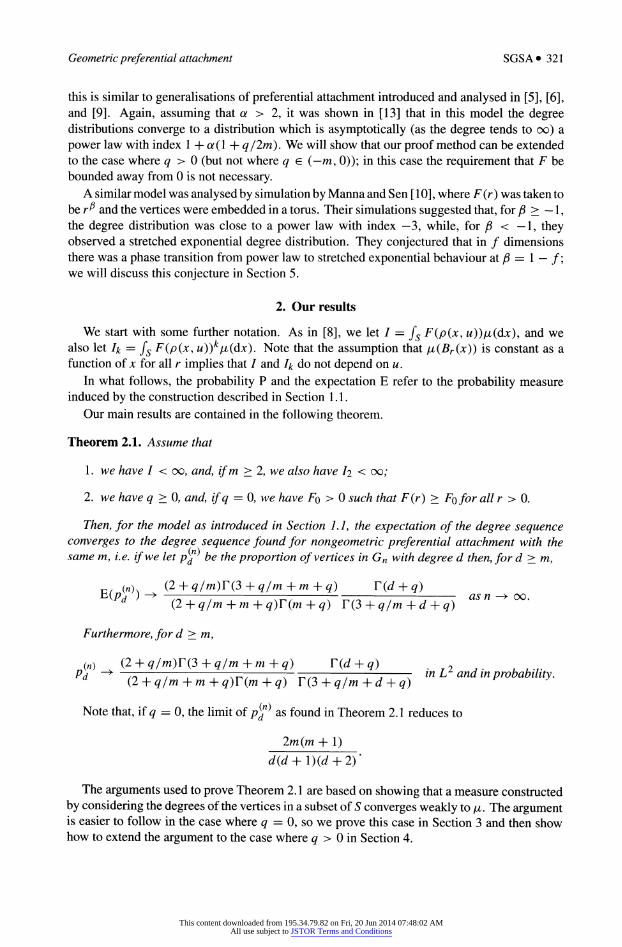
this is similar to generalisations of preferential attachment introduced and analysed in [5], [6], and [9]. Again, assuming that a > 2, it was shown in [13] that in this model the degree distributions converge to a distribution which is asymptotically (as the degree tends to oo) a
power law with index 1 + a (1 + q/2m). We will show that our proof method can be extended to the case where q > 0 (but not where q e (?ra, 0)); in this case the requirement that F be bounded away from 0 is not necessary.
A similar model was analysed by simulation by Manna and Sen [10], where F(r) was taken to be rP and the vertices were embedded in a torus. Their simulations suggested that, for 0 > ?
1, the degree distribution was close to a power law with index ?3, while, for ft < ?1, they observed a stretched exponential degree distribution. They conjectured that in / dimensions there was a phase transition from power law to stretched exponential behaviour at f$ = 1 ? /; we will discuss this conjecture in Section 5.
2. Our results
We start with some further notation. As in [8], we let I ? fs F(p(x, w))/x(d;c), and we also let Ik = fs F(p(x, u))kp,(dx). Note that the assumption that pi(Br(x)) is constant as a function of x for all r implies that / and 4 do not depend on u.
In what follows, the probability P and the expectation E refer to the probability measure induced by the construction described in Section 1.1.
Our main results are contained in the following theorem.
Theorem 2.1. Assume that
1. we have I < oo, and, ifm>2, we also have h < oo;
2. we have q > 0, and, if q = 0, we have Fo > 0 such that F(r) > Fofor all r > 0.
Then, for the model as introduced in Section 1.1, the expectation of the degree sequence converges to the degree sequence found for nongeometric preferential attachment with the same m, i.e. if we let p^ be the proportion of vertices in Gn with degree d then, for d > m,
(n) (2 + q/m)r(3 + q/m+m + q) V(d + q) E(p\ ) ?>-as n ?> oo. *d
(2 + q/m+m + q)T(m + q) T(3 + q/m + d + q)
Furthermore, for d > m,
(n) (2 + q/m)r(3 + q/m+m-r-q) T(d + q) . 2 Pj -> ??- -??-? ??- - in Z/ and in probability. ^d
(2 + q/m+m + q)r(m+q) r(3 + q/m + d + q)
Note that, if q = 0, the limit of p^ as found in Theorem 2.1 reduces to
2m (m + 1) d(d + \)(d + 2)'
The arguments used to prove Theorem 2.1 are based on showing that a measure constructed by considering the degrees of the vertices in a subset of S converges weakly to /x. The argument is easier to follow in the case where q = 0, so we prove this case in Section 3 and then show how to extend the argument to the case where q > 0 in Section 4.
This content downloaded from 195.34.79.82 on Fri, 20 Jun 2014 07:48:02 AMAll use subject to JSTOR Terms and Conditions

322?SGSA J. JORDAN
3. Proof of Theorem 2.1 when q = 0
In this section we prove some preliminary results, before putting them together to prove Theorem 2.1 in the case where q = 0.
We introduce a probability measure 8n on S given by
1 ^ 2(mn + ec\) ^ n
Then
?/ F(p(x,y))d^(y). 2(mrc + *?o)
Lemma 3.1. (a)7f
lim inf min P(V.(n+1) = u \ Fn)2(m" + gQ) > ^ far some K e (0, 1) "^oo MGy(Gn)
degGn(w)
/<?r awy AC5, P-almost surely,
liminf <$?(A) > 1
u(A). n^oo 2 -
(b)//
lim sup max P(V(w+1) = u | )2(m,g + gn) < L far some L e (1, 2) ?^oo mgV(G?) deggn(m)
then, for any ACS, wzY/z probability 1,
lim sup (A) < ?/z(A). n^oo L ? L
Proof We start by noting that
p(v^) = b|^) = e(^^^ fn) \ D?(Xn+i) )
= degG?E^ Dn{Xn+x) FHy
For (a), by the hypothesis,
p(V)("+1) = u | !Fn) >
1 ,rdegGn(?) 1
2(mn + eo)
for all m e V(G?), sufficiently large n, and any K' e [0, K). Then, for sufficiently large rc,
e(??+i (A) | JF?) = \ f degG? (v) + m P(X?+1 A)
2(m(n + l)+e0) V^^c,
+ m VJ T>(V?+l) = v\Fn))
^ ~, , ,\x-7(2(m" + e0)W) + mn(A) + mK'Sn(A)), 2(m(n + 1) + eo)
This content downloaded from 195.34.79.82 on Fri, 20 Jun 2014 07:48:02 AMAll use subject to JSTOR Terms and Conditions
Geometric preferential attachment SGSA 323
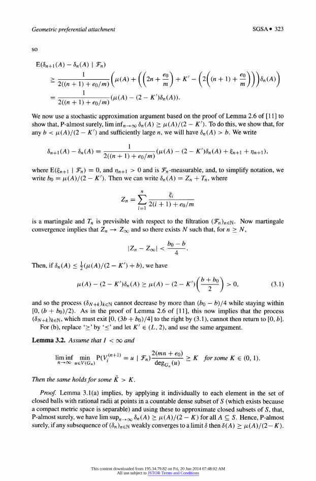
so
E(8n+l(A) - 8n(A) | Fn)
* +((2-+f)+r
- (2((-+0+
= 2,(? + 1)'+<!o/m)(>'(A>-(2-r>^(A)>
We now use a stochastic approximation argument based on the proof of Lemma 2.6 of [11] to show that, P-almost surely, lim inf 8n(A) > p(A)/(2
- K'). To do this, we show that, for
any b < p(A)/(2 ?
Kf) and sufficiently large n, we will have 8n(A) > b. We write
?n+i(A) - 8n(A) =
1 (p(A) - (2 - K')8n(A) + ?n+1 + nn+l),
2((n 4- 1) + eo/m)
where E(?w+i | J^) = 0, and nn+\ > 0 and is !Fn-measurable, and, to simplify notation, we
write bo = p(A)/(2 ?
Kf). Then we can write 8n(A) = Zn + Tn, where
z =Y"_^_ n ^ 2(/+ 1) +eo/m
is a martingale and Tn is previsible with respect to the filtration (!Fn)n?f$. Now martingale convergence implies that Zn -> Zqo and so there exists N such that, for n > Af,
|Zn -
Zoo| < ?-?.
Then, if 8n(A) < \(p(A)/(2 - Kr) + b), we have
p(A) -
(2 - > /x(A)
- (2
- > 0, (3.1)
and so the process (8N+k)keN cannot decrease by more than (bo ?
b)/4 while staying within
[0, (b + bo)/2). As in the proof of Lemma 2.6 of [11], this now implies that the process (?>N+k)keNi which must exit [0, (3b + bo)/4] to the right by (3.1), cannot then return to [0, b].
For (b), replace '>' by '<' and let K! e (L, 2), and use the same argument.
Lemma 3.2. Assume that I < oo and
liminf min P(y.("+1) = u \ Fn)1(\n +/o) > K for some K e (0, 1). n^oo ueV(Gn)
1 degGn(w)
~
Then the same holds for some K > K.
Proof Lemma 3.1(a) implies, by applying it individually to each element in the set of closed balls with rational radii at points in a countable dense subset of S (which exists because a compact metric space is separable) and using these to approximate closed subsets of S, that, P-almost surely, we have lim sup^^ 8n(A) > p(A)/(2
- K) for all A c S. Hence, P-almost
surely, if any subsequence of (8n)ne^ weakly converges to a limit 8 then 8 (A) > p(A)/(2 ?
K).
This content downloaded from 195.34.79.82 on Fri, 20 Jun 2014 07:48:02 AMAll use subject to JSTOR Terms and Conditions

324#SGSA J.JORDAN
As S is compact, this implies that, for K' <K,'\in is sufficiently large then, for all x,
^^ =
(Fo + /s(F(p(,,,))-Fo)d^))
>Fo + jzr^ js{F{p{x>y)) ~ Fo) df*iy)
t-i , I-Fo = Fo H 2 ? K'
= I + F0(l -
K') 2 ? K'
which implies that
limsup max P(vf+1> = u | Fn)^l?^ < <2 ~ n^oou V(Ga)
1 dtgGn(u) -I + F0(l-K)
2-K ~ 1 + F0(1-*)//'
Now let
L = max 1 + s, V l + Fo(l-K)/l)
for any sufficiently small e > 0; then L < 2 ? K. Then, similarly to above, Lemma 3.1(b) implies that
Dn(x) / + F0(1-L) hm sup- <-, n^oo 2(mn + eo) 2 - L
and so
liminf min P(vf+1> = u | ̂)2(m*
+ *o) > -^_= ?->oo M v(G?) 1
degGn(?) "
l-Fo(L-l)//
where 2-L
K =- > 2 - L > K.
1 - F0(L -
I)/1
Proposition 3.1. Under the hypotheses of Theorem 2.1 with q = 0, we have
r f Dn/("+i) i ̂ 2(mn + ^o) hm inf mm P(Vy = w | 5^) n-*oo ueV(Gn) degGn(?)
fw+n 2(mn + en) = limsup max P(V.(w+1) = w | F?) ?-= 1. ?_+oo u V(Gn) degGn(w)
Prat>/ We need to show that the hypothesis of Lemma 3.2 holds for some K e (0, 1); if we
can do this, we apply Lemma 3.2 to show that
hminf P(V;> = u \ Fn)?-?? = 1, n^oo
degGn(u)
because if this liminf is equal to some K e (0, 1), Lemma 3.2 then shows that it is equal to K > K, providing a contradiction. The argument in Lemma 3.2 shows that the lim sup must also be 1.
This content downloaded from 195.34.79.82 on Fri, 20 Jun 2014 07:48:02 AMAll use subject to JSTOR Terms and Conditions
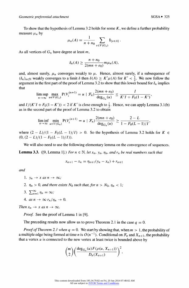
Geometric preferential attachment SGSA 325
To show that the hypothesis of Lemma 3.2 holds for some K, we define a further probability measure \in by
/Xn(A) = - -
V] l{veA} .
veV(Gn)
As all vertices of Gn have degree at least ra,
n + no &n(A) > ?-
--ra/xn(A), 2{mn + eo)
and, almost surely, [in converges weakly to [i. Hence, almost surely, if a subsequence of
(8n)neN weakly converges to a limit 8 then 8(A) > K'fi(A) for K' < \. We now follow the
argument in the first part of the proof of Lemma 3.2 to show that this lower bound for 8n implies that
lim sup max P(V.("+1) = u \ Fn)^ < ~r,-J~r*- .
n^JueV{Gn) Kl
degGn(u) -
K'I + Fo(\-KfY
and I/(KfI + Fo(l ?
Kr)) <2 '\fKr is close enough to \. Hence, we can apply Lemma 3.1(b) as in the second part of the proof of Lemma 3.2 to obtain
hminf mm P(V> = u \ Fn)?-?? >-??-7?7, n^oo ueV(Gn)
1 degGn(w) \-Fo(L-\)/I
where (2 -
L)/(l -
F0(L -
1)//) > 0. So the hypothesis of Lemma 3.2 holds for K e
(0, (2-L)/(l-F0(L-l)//)).
We will also need to use the following elementary lemma on the convergence of sequences.
Lemma 3.3. ([9, Lemma 1].) For n eN, let xn, yn, nn, and rn be real numbers such that
xn+i -xn = nn+i(yn
- xn) + r?+i
and
1. yn -> x as n ?> 00;
2. r\n > 0, and there exists No such that, for n > Afo, nn < 1;
3- J2T=\ tin = oo;
4. as n ?> 00 rn/t]n ?> 0.
Then xn ?> x as n ?> 00.
Proof See the proof of Lemma 1 in [9].
The preceding results now allow us to prove Theorem 2.1 in the case q = 0.
Proof of Theorem 2.1 when q =0. We start by showing that, when m > 1, the probability of a multiple edge being formed at time n is 0(n~l). Conditional on Fn and Xn+\, the probability that a vertex u is connected to the new vertex at least twice is bounded above by
/m\ /degGn(^F(p^,Xn+i))\2
\2J\ Dn(Xn+l) ) '
This content downloaded from 195.34.79.82 on Fri, 20 Jun 2014 07:48:02 AMAll use subject to JSTOR Terms and Conditions
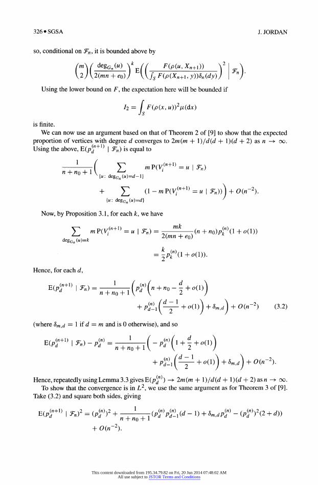
326* SGSA J.JORDAN
so, conditional on !Fn, it is bounded above by
(m\( degG>) \kE(( F(p(u,Xn+1)) \2 \ \2j\2(mn + eo)J \\fsF(p(Xn+uy))8n (dy)) n)'
Using the lower bound on F, the expectation here will be bounded if
h = jsF(p(x,u))2p(dx)
is finite. We can now use an argument based on that of Theorem 2 of [9] to show that the expected
proportion of vertices with degree d converges to 2m(m + \)/d(d + l)(d + 2) as n -> oo.
Using the above, EQ?^+1) | !Fn) is equal to
n + no + 1 V ' 1 >: degG?(?)=rf-l}
+ ? (1 - m P(^.("+1) = u | + 0{n-2).
{?: degG? (?)=</} '
Now, by Proposition 3.1, for each k, we have
T ?P(y/"+1)=H| y") = ,/ m\ An + n0)p{kn)(l+o(l)) degG>)=*
2(m"+e0)
= ^n)(l+0(D)
Hence, for each d,
E(^"+1) | Fn) = ?I?+?0 -
l+o(?) n + no + l\ \ 2 )
(where 8m,d = 1 if d = m and is 0 otherwise), and so
E<"i"+"'?-"?, = ^TT(-rf>(' + f + H
+ P{d\ + *(!))
+ <w)
+ tf("~2)
Hence, repeatedly using Lemma 3.3 gives E(p^) 2m(m + \)/d(d + l)(d + 2)asn -> oo.
To show that the convergence is in L2, we use the same argument as for Theorem 3 of [9]. Take (3.2) and square both sides, giving
E(/#+1) | f?f = ^2 + ^?(i-l)+W?)-(??))2(2 + * n+?o + l
+ 0(n-2).
This content downloaded from 195.34.79.82 on Fri, 20 Jun 2014 07:48:02 AMAll use subject to JSTOR Terms and Conditions

Geometric preferential attachment SGSA 327
As in [9], \p(;+l) -
pf\ = 0(n~l), so var(/#+1) | Fn) = 0(n~2), so
n I no I J
+ 0(?-2).
Hence, we can again use Lemma 3.3 repeatedly to show that, as n oo,
E(iP? } } -+ \d(d + l)(d+ 2)) '
giving the result.
4. Proof of Theorem 2.1 when q > 0
We will consider how the method of the previous section can be adapted to prove Theorem 2.1 in the case where q > 0. In this case the probability that = u conditional on Xn+\ and
Gn is
(degGnQ) +q)F(p(uJ Xn+\)) Dn(Xn+l)
where Dn(x) = EuGV(Gn)(degG? 0>) + q)F(p(v, x)).
Redefine the probability measure 8n by
2(mn + ^o)+^(n+no)w ^(G|i)
Then
-= / F(p(jc,y))d5n(y). 2(mn + eo) + ^(n + no)
To generalise Lemma 3.1(a), if we assume that, for all u e V(Gn), we have
/ degG (u) + q 2(mn + ^o) + q(n + no)
for some ^T' (0, 1), then
E(WA) | F?) > 1
( ^-?r 2(m(n + 1) + eo) + <?(rc + no + 1) x ((2(m/i + e0) + ? (n + n0))5n(A) + (ra + q)pi(A) + ra/T<5?(A)),
from which
E(?n+i(A) - ?n(A) | **) > | 2((w + 1) + ^o/w) + (q/m)(n + wo + 1)
x ((l
+ - 8n(A)(2 +1-
K^), so, P-almost surely,
1 + aim liminf &?(A) > m(A). n->oo 2 + q/m
? K
This content downloaded from 195.34.79.82 on Fri, 20 Jun 2014 07:48:02 AMAll use subject to JSTOR Terms and Conditions
328 SGSA J. JORDAN
Similarly, we can generalise Lemma 3.1(b) so that if, for all u e V(Gn), we have
P(V<^> ?u\fn)> K'-degG>)+g 2(mn + eo) + q(n + no)
for some V e (1, 2 + q/m), then, P-almost surely,
1 -f- a I m liminf 8n(A) < u(A). n-^oo 2 + q/m
? Z/
We now consider applying the proof of Lemma 3.2 to this case. Assuming that
r . f . t>/T/("+D i a- 2(mn + e0)+q(n + n0) lim inf mm P(Vy = u \ !Fn)- > K, n->oo ueV(Gn) degGn(?) + q
the same argument as before (with Fo = 0) will show that, for K' < K,
Dn(x) > 1(1+q/m) 2(mn + eo) + q(n + no)
~ 2 + q/m
? Kr'
which gives
r o/t/("+1) i *~ n 2(mn + go) + q(n + no) 2 + q/m - K
lim sup max P(V-V } = u \ !Fn)- <-,
n.+oo ueV(Gn) degGn(?)+^ l+q/m
so we let _ 2 +q/m
- K
l+q/m Then, adapting the last part of the proof of Lemma 3.2 shows that
r , . t>/t/("+l) .?2(mn + eo)+q(n+no)^~ 2 + q/m ? L
lim inf mm P(Vy = u \ !Fn)- > K =-. n-+oo ueV(Gn) degGn(w)+4 (l+q/m)
Now
g _ 2 + q/m -(2 + q/m - K)/(l + q/m) _ (q/m)2 + 2q/m + K ~
l+q/m ~
(l+q/m)2
To use the same argument as in Section 3, we require that K > K for all K < 1. To check this,
y K _ (q/m)2 + 2q/m + K-K(l+ q/m)2 K~ (l+q/m)2
_ (1- K)(q/m)2 + 2(1- K)q/m (l+q/m)2
= (l-^)(l+^/m)2-(l-^)
(l+q/m)2
so K ? K is always positive for K < 1 if q > 0.
Next, we need to consider the argument in Proposition 3.1. The lower bound on 8n(A) becomes
(n+n0)(m + q) 8n(A) > ?-
?rMn(A), 2(mn + eo) + q(n + no)
This content downloaded from 195.34.79.82 on Fri, 20 Jun 2014 07:48:02 AMAll use subject to JSTOR Terms and Conditions

Geometric preferential attachment SGSA 329
so, for any subsequential weak limit of (5n)WGN> we have 8(A) > K' p(A) for Kf < (ra +
q)/(2m + g), which will give
hmsup max P(V> = u \ Fn)-?- < ?-, n^oo ueV(Gn)
1 dtgGn(u) + q Kf
and \/Kf < 2 + q/m if K' is close enough to (m + q)/(2m + g). Hence, the hypothesis of the modified Lemma 3.2 will hold for some K > 0.
The argument that the probability of forming multiple edges is 0(n~l) will be the same, with the same condition. The rest of the proof will be essentially the same as before, giving
(?) (2 + q/m)T(3 + q/m + m+q) T(d + q) Pd ~*
(2 + q/m+m+q)Y(m + q) V(3 + q/m+d + q)
in L2 as n ?> oo.
5. Discussion and open questions
In [10], it was conjectured, based on simulations, that, with F(r) = r^, in / dimensions there is a phase transition from power law to stretched exponential behaviour of the degree distribution at f$ = 1 ? /. With this choice of F, / is finite for f> >
? /, so our results imply
that (for m = 1) if there is a phase transition at some /3C then fic < ?/, suggesting that, if there is a phase transition, it occurs at a lower f> than conjectured in [10]. The plots of the
proportion of degree 1 vertices in [10] do appear to be consistent with a slow convergence to the Barabasi-Albert distribution for f> < ?f with a phase transition at f> = ?f.
Open questions include whether we can say anything about the case where / is infinite; the simulation results in [10] suggest that the degree distribution can be different in this case. Other
questions include whether the assumption that F is bounded away from 0, which is important to our proof method, is necessary, assuming the initial configuration is such that Dn (x) is never 0, and whether the assumption that h =
fs F(p(x, u))2p(dx) finite is necessary if m > 1. The model also makes sense with the initial attractiveness q e (?ra, 0), but our proof method does not seem to work in this case, so another question is whether the results hold with negative q.
We also pose the question of whether similar results apply in some cases when the measure
/x does not satisfy the condition that, for any fixed r, p(Br(x)) is constant as a function of jc, for example a uniform measure on a square, or a nonuniform measure on a sphere or torus.
Acknowledgements
The author would like to acknowledge the support of the EPSRC funded Amorphous Computing, Random Graphs and Complex Biological Systems group (grant reference number
EP/D003105/1), and would also like to thank John Biggins for some useful discussions while the paper was being written and an anonymous referee for pointing out that the conditions on F in the original version of this paper could be weakened.
References
[1] Barabasi, A.-L., Albert, R. and Jeong, H. (1999). Mean-field theory for scale-free random networks. Physica A 272, 173-187.
[2] Barnett, L., Di Paolo, E. and Bullock, S. (2007). Spatially embedded random networks. Phys. Rev. E 76, 056115, 18 pp.
[3] Bollobas, B. and Riordan, O. (2004). The diameter of a scale-free random graph. Combinatorica 24,5-34.
This content downloaded from 195.34.79.82 on Fri, 20 Jun 2014 07:48:02 AMAll use subject to JSTOR Terms and Conditions

330*SGSA J. JORDAN
[4] Bollobas, B., Riordan, O., Spencer, J. and Tusnady, G. (2001). The degree sequence of a scale-free random
graph process. Random Structures Algorithms 18, 279-290.
[5] Deijfen, M., van den Esker, H., van der Hofstad, R. and Hooghiemstra, G. (2009). A preferential attachment model with random initial degrees. Ark. Mat. 47,41-72.
[6] Dorogovtsev, S. N., Mendes, J. F. R and Samukhin, A. N. (2000). Structure of growing networks with
preferential linking. Phys. Rev. Lett. 85,4633-4636. [7] Flaxman, A. D., Frieze, A. M. and Vera, J. (2006). A geometric preferential attachment model of networks.
Internet Math. 3, 187-206.
[8] Flaxman, A. D., Frieze, A. M. and Vera, J. (2007). A geometric preferential attachment model of networks
II. Internet Math. 4, 87-112.
[9] Jordan, J. (2006). The degree sequences and spectra of scale-free random graphs. Random Structures Algorithms
29, 226-242.
[10] Manna, S. S. and Sen, P. (2002). Modulated scale-free network in Euclidean space. Phys. Rev. E 66,066114.
[11] Pemantle, R. (2007). A survey of random processes with reinforcement. Prob. Surveys 4, 1-79.
[12] Penrose, M. (2003). Random Geometric Graphs. Oxford University Press.
[13] Van der Esker, H. (2008). A geometric preferential attachment model with fitness. Preprint. Available at
http://arxiv.org/abs/0801.1612.
This content downloaded from 195.34.79.82 on Fri, 20 Jun 2014 07:48:02 AMAll use subject to JSTOR Terms and Conditions