Delay Minimal Policies in Energy Harvesting …ulukus/papers/journal/delay-min-eh.pdf · ARAFA et al.: DELAY MINIMAL POLICIES IN ENERGY HARVESTING COMMUNICATION SYSTEMS 2923 Fig

2918 IEEE TRANSACTIONS ON COMMUNICATIONS, VOL. 66, NO. 7, JULY 2018

Delay Minimal Policies in Energy HarvestingCommunication Systems

Ahmed Arafa , Member, IEEE, Tian Tong, Minghan Fu, Sennur Ulukus , Fellow, IEEE,

and Wei Chen , Senior Member, IEEE

Abstract— We characterize delay minimal power schedulingpolicies in energy harvesting communication systems. We con-sider a continuous-time system, where the delay experienced byeach bit is given by the time spent by the bit in the queue waitingto be transmitted to its receiver. We first consider a single-user channel, where the transmitter has a finite-sized batteryto save its harvested energy. Data arrives during the course ofcommunication and are saved in a finite data buffer as well.We find the optimal power policy that minimizes the averagedelay experienced by the bits subject to energy and data causalityconstraints. We characterize the optimal solution in terms ofLagrange multipliers, and calculate their values in a recursivemanner. We show that, different from the existing literature,the optimum transmission power is not constant between theenergy and data arrival events; the transmission power startshigh, decreases linearly, and potentially reaches zero betweenenergy and data arrivals. Intuitively, untransmitted bits experi-ence cumulative delay due to the bits to be transmitted aheadof them, and hence the reason for transmission power startinghigh and decreasing over time. Next, we study a multiuserversion of this problem, namely, a two-user broadcast channel,and characterize the optimal transmission policies that minimizethe sum delay. For this setting, we consider the case, where thetransmitter has an infinite-sized battery, and that all data packetsintended for the receivers are available at the beginning of thecommunication session. We characterize the optimal solution interms of Lagrange multipliers, and present an iterative solutionthat calculates their values. Our results show that in the optimalpolicy, both users may not be served simultaneously all the time;

Manuscript received July 30, 2017; revised December 18, 2017; acceptedJanuary 26, 2018. Date of publication February 12, 2018; date of currentversion July 13, 2018. This work was supported by NSF under GrantCNS 13-14733, Grant CCF 14-22111, and Grant CNS 15-26608. This paperwas presented in part at the IEEE International Conference on Communica-tions, London, England, June 2015 [1], and in part at the IEEE InternationalConference on Communications, Kuala Lumpur, Malaysia, May 2016 [2].The associate editor coordinating the review of this paper and approving itfor publication was V. Stankovic. (Corresponding author: Sennur Ulukus.)

A. Arafa was with the Department of Electrical and Computer Engineering,University of Maryland at College Park, College Park, MD 20742 USA.He is now with the Department of Electrical Engineering, Princeton Uni-versity, Princeton, NJ 08544 USA (e-mail: [email protected]).

T. Tong is with the Electrical and Computer Engineering Depart-ment, Carnegie Mellon University, Pittsburgh, PA 15213 USA (e-mail:[email protected]).

M. Fu was with the Computer Science Department, Carnegie MellonUniversity, Pittsburgh, PA 15213 USA. She is now with Snap Inc., Venice,CA 90291 USA (e-mail: [email protected]).

S. Ulukus is with the Department of Electrical and Computer Engineering,University of Maryland at College Park, College Park, MD 20742 USA(e-mail: [email protected]).

W. Chen is with the Department of Electronic Engineering, TsinghuaUniversity, Beijing 100084, China (e-mail: [email protected]).

Color versions of one or more of the figures in this paper are availableonline at http://ieeexplore.ieee.org.

Digital Object Identifier 10.1109/TCOMM.2018.2805357

there may be times, where only one of the two users is servedalone. We also show that the optimal policy may have gaps intransmission in between energy arrivals, where none of the usersis served, echoing the results of the single-user setting.

Index Terms— Energy harvesting, delay minimization, single-user channel, broadcast channel, finite battery, finite buffer.

I. INTRODUCTION

WE CONSIDER energy harvesting communicationsystems where the transmitter relies solely on energy

harvested from nature to maintain the power necessary for datatransmission. According to a specific data demand, the trans-mitter needs to schedule the transmission of data packets usingthe available energy such that the average delay experiencedby the data is minimal.

Optimal resource allocation and scheduling policies havebeen considered for various energy harvesting communicationmodels. Earlier works focus on throughput maximization andtransmission completion time minimization policies for single-user settings [3]–[6], broadcast channels [7]–[9], multipleaccess channels [10], interference channels [11], relay chan-nels [12]–[15], and settings with energy cooperation [16].In addition, energy leakage from battery over time [17], batteryinefficiency at the time of charging [18], systems with hybridenergy storage [19], processing costs [20], [21], and receiverdecoding costs [22], [23] have been considered.

In [3], the problem of minimizing the transmission com-pletion time is considered. Reference [3] and the subsequentliterature showed that, due to the concavity of the rate-power relationship, the transmit power must be kept constantbetween energy harvesting and data arrival events, and thetransmitter must schedule data transmissions using longestpossible stretches of constant power, subject to energy and datacausality. While [3] minimizes the time by which all of thedata packets are transmitted, different data packets experiencedifferent delays, and the average delay of the system isnot minimized. In particular, when the earlier-arriving datapackets are transmitted slowly, the later-arriving data packetsexperience not only the delay in their own transmissions,but a portion of the delay experienced by the earlier-arrivingpackets, as they have to wait extra time in the data queuewhile those packets are being transmitted. This compoundsthe delays that the later-arriving data packets experience. Thedelay minimization problem was considered previously in [24]for a non energy harvesting system.

0090-6778 © 2018 IEEE. Personal use is permitted, but republication/redistribution requires IEEE permission.See http://www.ieee.org/publications_standards/publications/rights/index.html for more information.

https://orcid.org/0000-0003-2032-1840

https://orcid.org/0000-0002-8219-8190

https://orcid.org/0000-0002-9066-1448

ARAFA et al.: DELAY MINIMAL POLICIES IN ENERGY HARVESTING COMMUNICATION SYSTEMS 2919

In this paper, we consider the problem of average delay min-imization in an energy harvesting system. First, we considera single-user channel where the transmitter is equipped witha finite-sized battery and a finite-sized data buffer. We showthat, unlike the previous literature, the transmission powershould not be kept constant between energy harvesting anddata arrival events. We let the power (and therefore the rate)vary even during the transmission of a single packet. We showthat the optimal packet scheduling is such that the transmitpower starts with a high value and decreases linearly overtime possibly reaching zero before the arrival of the nextenergy or data packet into the system. The high initial transmitpower values ensure that earlier bits are transmitted faster,decreasing their own delay and also the delays of the later-arriving data packets. We develop a recursive solution thatfinds the optimal transmit power over time by determining theoptimal Lagrange multipliers.

Next, we consider a two-user energy harvesting broadcastchannel where the transmitter is equipped with an infinite-sized battery, and data packets intended for both users areavailable before the transmission starts. In this system, thereis a tradeoff between the delays experienced by both users;as more resources (power) is allocated to a user, its delaydecreases while the delay of the other user increases. We con-sider the minimization of the sum delay in the system.We formulate the problem using a Lagrangian framework, andexpress the optimal solution in terms of Lagrange multipliers.We develop an iterative solution that solves the optimumLagrange multipliers by enforcing the KKT optimality condi-tions. Similar to the single-user setting, we show that the opti-mal transmission power decreases between energy harvests,and may possibly hit zero before the next energy harvest,yielding communication gaps, where no data is transmitted.During active communication, data may be sent to bothusers, or only to the stronger user, or only to the weaker user,depending on the energy harvesting profile. We contrast ourwork with [7] which developed an algorithm that minimizesthe transmission completion time, i.e., a time by which all datais delivered to users. To that end, [7] studies the throughputmaximization problem, and shows that, for general user prior-ities, there exists a cut-off power level such that only the totalpower above this level is used to serve the weaker user. In par-ticular, for sum throughput maximization, this cut-off is infin-ity, and all power is allocated to packets sent to the strongeruser. In contrast, in our sum delay minimization problem,the weaker user always gets a share of the transmitted power,as otherwise, its delay becomes unbounded, and the sum delaywill not be minimized. In our work, we show that there existsa cut-off time, beyond which data is sent only to the weakeruser.

II. SINGLE-USER CHANNEL

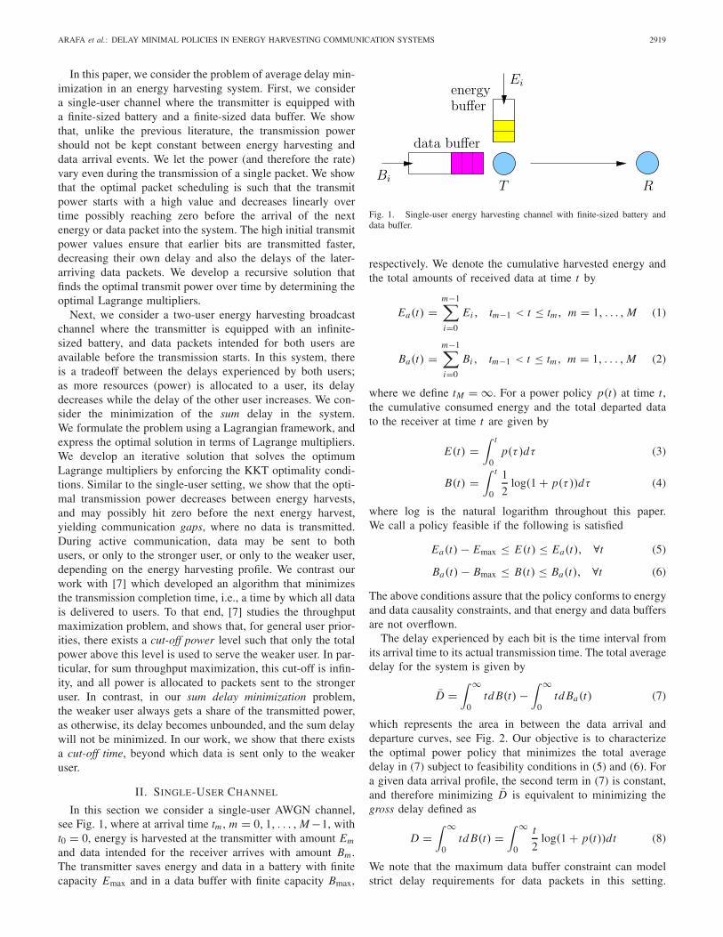
In this section we consider a single-user AWGN channel,see Fig. 1, where at arrival time tm , m = 0, 1, . . . , M −1, witht0 = 0, energy is harvested at the transmitter with amount Em

and data intended for the receiver arrives with amount Bm .The transmitter saves energy and data in a battery with finitecapacity Emax and in a data buffer with finite capacity Bmax,

Fig. 1. Single-user energy harvesting channel with finite-sized battery anddata buffer.

respectively. We denote the cumulative harvested energy andthe total amounts of received data at time t by

Ea(t) =m−1∑

i=0

Ei , tm−1 < t ≤ tm, m = 1, . . . , M (1)

Ba(t) =m−1∑

i=0

Bi , tm−1 < t ≤ tm, m = 1, . . . , M (2)

where we define tM = ∞. For a power policy p(t) at time t ,the cumulative consumed energy and the total departed datato the receiver at time t are given by

E(t) =∫ t

0p(τ )dτ (3)

B(t) =∫ t

0

1

2log(1 + p(τ ))dτ (4)

where log is the natural logarithm throughout this paper.We call a policy feasible if the following is satisfied

Ea(t) − Emax ≤ E(t) ≤ Ea(t), ∀t (5)

Ba(t) − Bmax ≤ B(t) ≤ Ba(t), ∀t (6)

The above conditions assure that the policy conforms to energyand data causality constraints, and that energy and data buffersare not overflown.

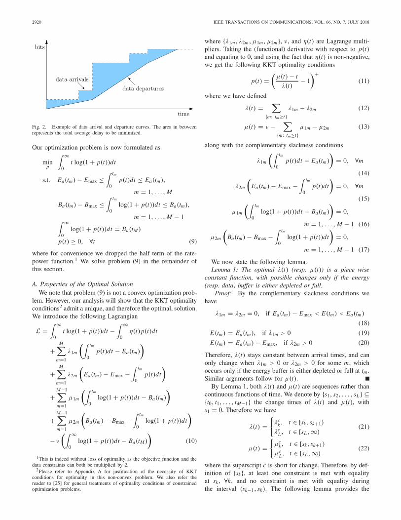
The delay experienced by each bit is the time interval fromits arrival time to its actual transmission time. The total averagedelay for the system is given by

D̄ =∫ ∞

0td B(t) −

∫ ∞

0td Ba(t) (7)

which represents the area in between the data arrival anddeparture curves, see Fig. 2. Our objective is to characterizethe optimal power policy that minimizes the total averagedelay in (7) subject to feasibility conditions in (5) and (6). Fora given data arrival profile, the second term in (7) is constant,and therefore minimizing D̄ is equivalent to minimizing thegross delay defined as

D =∫ ∞

0td B(t) =

∫ ∞

0

t

2log(1 + p(t))dt (8)

We note that the maximum data buffer constraint can modelstrict delay requirements for data packets in this setting.


Fig. 2. Example of data arrival and departure curves. The area in betweenrepresents the total average delay to be minimized.

Our optimization problem is now formulated as

minp

∫ ∞

0t log(1 + p(t))dt

s.t. Ea(tm) − Emax ≤∫ tm

0p(t)dt ≤ Ea(tm),

m = 1, . . . , M

Ba(tm) − Bmax ≤∫ tm

0log(1 + p(t))dt ≤ Ba(tm),

m = 1, . . . , M − 1∫ ∞

0log(1 + p(t))dt = Ba(tM )

p(t) ≥ 0, ∀t (9)

where for convenience we dropped the half term of the rate-power function.1 We solve problem (9) in the remainder ofthis section.

A. Properties of the Optimal SolutionWe note that problem (9) is not a convex optimization prob-

lem. However, our analysis will show that the KKT optimalityconditions2 admit a unique, and therefore the optimal, solution.We introduce the following Lagrangian

L =∫ ∞

0t log(1 + p(t))dt −

∫ ∞

0η(t)p(t)dt

+M∑

m=1

λ1m

(∫ tm

0p(t)dt − Ea(tm)

)

+M∑

m=1

λ2m

(Ea(tm) − Emax −

∫ tm

0p(t)dt

)

+M−1∑

m=1

μ1m

(∫ tm

0log(1 + p(t))dt − Ba(tm)

)

+M−1∑

m=1

μ2m

(Ba(tm) − Bmax −

∫ tm

0log(1 + p(t))dt

)

− ν

(∫ ∞

0log(1 + p(t))dt − Ba(tM )

)(10)

1This is indeed without loss of optimality as the objective function and thedata constraints can both be multiplied by 2.

2Please refer to Appendix A for justification of the necessity of KKTconditions for optimality in this non-convex problem. We also refer thereader to [25] for general treatments of optimality conditions of constrainedoptimization problems.

where {λ1m, λ2m , μ1m, μ2m}, ν, and η(t) are Lagrange multi-pliers. Taking the (functional) derivative with respect to p(t)and equating to 0, and using the fact that η(t) is non-negative,we get the following KKT optimality conditions

p(t) =(

μ(t) − t

λ(t)− 1

)+(11)

where we have defined

λ(t) =∑

{m: tm≥t}λ1m − λ2m (12)

μ(t) = ν −∑

{m: tm≥t}μ1m − μ2m (13)

along with the complementary slackness conditions

λ1m

(∫ tm

0p(t)dt − Ea(tm)

)= 0, ∀m

(14)

λ2m

(Ea(tm) − Emax −

∫ tm

0p(t)dt

)= 0, ∀m

(15)

μ1m

(∫ tm

0log(1 + p(t))dt − Ba(tm)

)= 0,

m = 1, . . . , M − 1 (16)

μ2m

(Ba(tm) − Bmax −

∫ tm

0log(1 + p(t))dt

)= 0,

m = 1, . . . , M − 1 (17)

We now state the following lemma.Lemma 1: The optimal λ(t) (resp. μ(t)) is a piece wise

constant function, with possible changes only if the energy(resp. data) buffer is either depleted or full.

Proof: By the complementary slackness conditions wehave

λ1m = λ2m = 0, if Ea(tm) − Emax < E(tm) < Ea(tm)

(18)

E(tm) = Ea(tm), if λ1m > 0 (19)

E(tm) = Ea(tm) − Emax, if λ2m > 0 (20)

Therefore, λ(t) stays constant between arrival times, and canonly change when λ1m > 0 or λ2m > 0 for some m, whichoccurs only if the energy buffer is either depleted or full at tm .Similar arguments follow for μ(t).

By Lemma 1, both λ(t) and μ(t) are sequences rather thancontinuous functions of time. We denote by {s1, s2, . . . , sL} ⊆{t0, t1, . . . , tM−1} the change times of λ(t) and μ(t), withs1 = 0. Therefore we have

λ(t) ={

λck, t ∈ [sk, sk+1)

λcL , t ∈ [sL,∞)

(21)

μ(t) ={

μck, t ∈ [sk, sk+1)

μcL, t ∈ [sL ,∞)

(22)

where the superscript c is short for change. Therefore, by def-inition of {sk}, at least one constraint is met with equalityat sk , ∀k, and no constraint is met with equality duringthe interval (sk−1, sk). The following lemma provides the


necessary conditions for the two sequences {λck} and {μc

k} toincrease/decrease.

Lemma 2: In the optimal policy: 1) λck > λc

k−1 (resp. λck <

λck−1) only if the battery is full (resp. depleted) at time sk−1;

and 2) μck > μc

k−1 (resp. μck < μc

k−1) only if the data bufferis depleted (resp. full) at time sk−1.

Proof: By definition of λ(t) in (12), the function can onlyincrease (resp. decrease) after time sk−1 if λ2m > 0 (resp.λ1m > 0) for m such that tm = sk−1. By complementaryslackness, the battery must be full (resp. depleted) at time sk−1.The second statement of the lemma follows using similararguments.

We conclude the optimality conditions by the followinglemma.

Lemma 3: Whenever the optimal power p(t) > 0 on someopen interval in between arrival times, it is monotonicallydecreasing.

Proof: Let us have p(t) > 0 ∀t ∈ (l1, l2) where (l1, l2)lies in between arrival times. By Lemma 1, we know thatboth λ(t) and μ(t) are constants during that interval (sayλl and μl). Hence, from (11), p(t) is either monotonicallyincreasing or decreasing (depending on the sign of λl ). Nowassume it is increasing during this interval, i.e., λl < 0, anddenote λ′

l = −λl , and μ′l = l2 − μl + l1. Now define a new

power policy p′(t) = (μ′l − t)/λ′

l − 1, for t ∈ (l1, l2). It isdirect to see that both p(t) and p′(t) use the same energy anddeliver the same data amount during (l1, l2), as what we didis merely flipping the curve of p(t) in (l1, l2) around l1+l2

2 .However, the (now decreasing) new policy p′(t) does so witha strictly less delay. This is due to the multiplicative term t inthe objective function; it is strictly better to use higher powersat the beginning and lower powers at the end, so that dataarriving earlier in time are delivered faster.

By Lemma 3, we conclude that the optimal λ(t) is non-negative for all t , and that it is necessary, from (11), to haveμ(t) > t for all t before the total amount of data isdelivered. Lemma 3 also shows that power can reach 0 inbetween arrivals, where the communication stops until the nextenergy or data arrival instant.

B. Recursive Formulas

In this section, we show how to find λck , μc

k , and sk ina recursive manner. We will use these recursive formulas toconstruct the optimal solution in the next section. First, assumesk , E(sk), B(sk), and μc

k are known, and define the followingvalues for all {m : tm > sk}

λeum : E(sk) +

∫ tm

sk

(μc

k − t

λeum

− 1

)+dt = Ea(tm) (23)

λbum : B(sk) +

∫ tm

sk

log

(1 +

(μc

k − t

λbum

− 1

)+)dt = Ba(tm)

(24)

λum = max{λeu

m , λbum } (25)

λelm : E(sk) +

∫ tm

sk

(μc

k − t

λelm

− 1

)+dt = Ea(tm) − Emax

(26)

λblm : B(sk)+

∫ tm

sk

log

(1+

(μc

k −t

λblm

−1

)+)

dt = Ba(tm)−Bmax

(27)

λlm = min{λel

m , λblm } (28)

Therefore, λum is the minimum value of λ such that either the

energy or the data buffer is depleted by time tm , i.e., an upperbound is met with equality. On the other hand, λl

m is the max-imum value of λ such that either the energy or the data bufferis full by time tm , i.e., a lower bound is met with equality.Observe that these values are unique, by monotonicity of theintegrands on the left hand side of the above equations. Letus denote �(m) = [λu

m , λlm ]. Hence, to maintain feasibility,

we need to have λck ∈ �(m) if sk+1 ≥ tm . Now define the

following integers

mmax1 (k) = max

⎧⎨

⎩m :m⋂

i: ti>sk

�(i) = ∅⎫⎬

⎭ (29)

mu1(k) = max

⎧⎨

⎩m : λum ∈

m⋂

i: ti>sk

�(i)

⎫⎬

⎭ (30)

ml1(k) = max

⎧⎨

⎩m : λlm ∈

m⋂

i: ti>sk

�(i)

⎫⎬

⎭ (31)

We now have the following lemma; with the assumption thatthe optimal solution of the problem is only partially revealedup to a given time, it provides a method to proceed forwardand find the optimal solution up to some specific future time.

Lemma 4: Assume that one has the optimal solution up totime sk , along with μc

k . Then, λck and sk+1 are found as follows:

If �(mmax

1 (k) + 1)

>

mmax1 (k)⋂

i: ti>sk

�(i)

⇒ λck = λl

ml1(k)

, sk+1 = tml1(k)

Else, if �(mmax

1 (k) + 1)

<

mmax1 (k)⋂

i: ti>sk

�(i)

⇒ λck = λu

mu1 (k), sk+1 = tmu

1 (k)

where the comparisons of the intervals above are pointwise.3

Proof: Let us assume that �(mmax

1 (k) + 1)

>⋂mmax

1 (k)

i: ti>sk�(i) and consider two different possibilities. First,

if λck > λl

ml1(k)

, then a lower bound will be met before tml1(k).

By Lemma 2, we know that λ(t) can only increase if a lowerbound is met with equality. This means that eventually thelower bound at tml

1(k) will be breached. On the other hand,

if λck < λl

ml1(k)

, then by definition of ml1(k), we know that

λlm ≥ λl

ml1(k)

for all m : sk < tm < ml1(k). This means

that only an upper bound can be met before or at tml1(k).

3By [a1, a2] > [b1, b2] we mathematically mean that a1 > b2, andinversely by [a1, a2] < [b1, b2] we mathematically mean that a2 < b1.Note that by definition of mmax

1 (k), the two intervals �(mmax

1 (k) + 1)

and⋂mmax

1 (k)i: ti >sk

�(i) have no intersection, and thus the two cases considered in thelemma are mutually exclusive.


By Lemma 2, we know that λ(t) can only decrease if an upperbound is met with equality. Therefore, λ(t) will not increaseto have a value inside �

(mmax

1 (k) + 1)

(which lies above⋂mmax

1 (k)

i: ti>sk�(i) by assumption) at tmmax

1 (k)+1, i.e., the upperbound at tmmax

1 (k)+1 will be breached. Thus, we must have λck =

λlml

1(k), sk+1 = tml

1(k) in this case. Similar arguments follow

for the other case when �(mmax

1 (k) + 1)

<⋂mmax

1 (k)

i: ti>sk�(i).

Similarly to what we did above, we can define the quantities{μeu

m , μbum , μu

m , μelm , μbl

m , μlm} as we did in (23)-(28) with fixed

(known) λck . Further, we can also define the set U(m) =

[μlm, μu

m ], which gives rise to the following integers

mmax2 (k) = max

⎧⎨

⎩m :m⋂

i: ti>sk

U(i) = ∅⎫⎬

⎭ (32)

mu2(k) = max

⎧⎨

⎩m : μum ∈

m⋂

i: ti>sk

U(i)

⎫⎬

⎭ (33)

ml2(k) = max

⎧⎨

⎩m : μlm ∈

m⋂

i: ti>sk

U(i)

⎫⎬

⎭ (34)

We now have the following lemma, complementing and serv-ing the same purpose as Lemma 4. The proof follows usingsimilar arguments as in that of Lemma 4, and is thereforeomitted for brevity.

Lemma 5: Assume that one has the optimal solution up totime sk , along with λc

k . Then, μck and sk+1 are found as follows

If U(mmax

2 (k) + 1)

>

mmax2 (k)⋂

i: ti>sk

U(i)

⇒ μck = μu

mu2 (k), sk+1 = tmu

2 (k)

Else, if U(mmax

2 (k) + 1)

<

mmax2 (k)⋂

i: ti>sk

U(i)

⇒ μck = μl

ml2(k)

, sk+1 = tml2(k)

where the comparisons of the intervals above are pointwise.Lemmas 4 and 5 show how to optimally construct λc

kand μc

k , along with sk+1, given μck and λc

k , respectively,along with the optimal solution up to sk . In solving ourproblem, we neither know the optimal value of λc

1 or μc1 in

order to apply those lemmas, and hence, we need to assumesome initialization values for either of them in order to startcomputing the remaining ones recursively. It then remains tofind out if such initializations were erroneous, and how toadjust them if this were the case. In addition to that issue,we also note that Lemmas 4 and 5 only give the valueof sk+1. One needs either λc

k+1 or μck+1 along the way in

order to reapply the results of the lemmas and move forwardto find sk+2. We address these issues formally through the nextseries of lemmas. Throughout the lemmas, we first assume avalue for μc

k and find the corresponding values of λck and

sk+1 by Lemma 4. We then assess the optimality of theassumed μc

k according to the constraints met at sk+1. The next

lemma will help in that assessment. We provide its proof inAppendix B.

Lemma 6: Given a time interval [s, s̄], and a decreasingpower policy p0(t), if we define another decreasing powerpolicy p1(t) that consumes the same amount of energy dur-ing [s, s̄], and has a slower decline, i.e., has a larger slope,then the policy p1(t) departs more data during that interval.Similarly, if we define another power policy p2(t) that departsthe same amount of data during [s, s̄], and has a slowerdecline, i.e., has a larger slope, then the policy p2(t) consumesless energy during that interval.

Next, we use the results in Lemma 6 to prove the state-ments in the following lemmas. Throughout the lemmas,as mentioned previously, we assess the optimality of anassumed value of μc

k based on how the constraints at sk+1are met/violated. We provide proofs of these lemmas inAppendices C through F.

Lemma 7: If an energy constraint is binding at sk+1, whiledata constraints are not, and if μc

k > sk+1, then we haveμc

k+1 = μck . Otherwise, μc

k is not optimal, and needs toincrease. Similarly, if a data constraint is binding at sk+1,while energy constraints are not, and if sk+1 < tM = ∞, thenwe have λc

k+1 = λck . Otherwise, μc

k is not optimal, and needsto decrease.

Lemma 8: If the battery is empty at sk+1, and the databuffer is overflown, then μc

k is not optimal and needs toincrease. Similarly, if the data buffer is empty at sk+1, andthe battery is overflown, then μc

k is not optimal and needs todecrease.

The next two lemmas deal with the cases where both dataand energy constraints are binding at sk+1. In such cases,we re-solve a shifted problem starting at sk+1 recursivelyusing the above analysis, with initial conditions as indicated bythe binding constraints at sk+1, e.g., a full/empty data/energybuffer, and denote the optimal Lagrange multipliers of thisshifted problem by {λ̄i , μ̄i }M

i=k+1. We then compare the val-ues of those Lagrange multipliers obtained from the shiftedproblem to λc

k and μck and examine their optimality as follows.

Lemma 9: If the battery is empty (resp. full) and the databuffer is full (resp. empty) at sk+1, and the solution of theshifted problem satisfies: λ̄k+1 ≤ λc

k and μ̄k+1 ≤ μck (resp.

λ̄k+1 ≥ λck and μ̄k+1 ≥ μc

k), then the solution of the shiftedproblem, as well as the pair {λc

k, μck}, is optimal. Otherwise,

μck is not optimal and needs to increase (resp. decrease).Lemma 10: If both the battery and the data buffer are empty

(resp. full) at sk+1, and the solution of the shifted problemsatisfies: λ̄k+1 ≤ λc

k and μ̄k+1 ≥ μck (resp. λ̄k+1 ≥ λc

k andμ̄k+1 ≤ μc

k), then the solution of the shifted problem, as wellas the pair {λc

k, μck}, is optimal. Otherwise, if λ̄k+1 > λc

k (resp.μ̄k+1 > μc

k), then μck is not optimal and needs to increase.

On the other hand, if μ̄k+1 < μck (resp. λ̄k+1 < λc

k ), then μck

is not optimal and needs to decrease.It is clear from the above recursive formulas that the

optimal Lagrange multipliers can only have one unique setof values. For instance, equations (23)-(28) constitute themethod of computing the Lagrange multipliers from oneepoch to the next. In there, we note that the left handsides are all monotone in λm given μc

k is fixed, and vice


Fig. 3. Two-user energy harvesting broadcast channel.

versa. Since our solution approach is based on fixing oneparameter and finding the other one through these equations inLemma 4 (and their complements in Lemma 5), we concludethat the KKT conditions have a unique solution for thisproblem, as mentioned in the beginning of the analysis inSection II-A. We summarize the proposed algorithmic solutionnext.

C. Constructing the Optimal Solution

In this section, we summarize the solution of the single-userproblem. We first initialize by setting s1 = 0, and choosing avalue for μc

1. We then find the value of λc1 and s1 by Lemma 4.

Next, we check the constraints at s1 and use Lemmas 7, 8, 9,and 10 to assess the optimality of the initialized μc

1. Thisresults into one of the following cases: 1) the value of μc

2 or λc2

is given because μc1 is optimal; 2) μc

1 is not optimal andneeds to increase or decrease; 3) the optimal solution of theproblem is obtained according to Lemmas 9 and 10. In case 3,we need to solve a shifted problem starting at s2; we doso by initializing a value of μc

2 and continue as discussedabove. In case 2, one can find the optimal μc

1 by using,e.g., a bisection search. In case 1, we either use Lemma 4to find λc

2 and s3 if μc2 was given, or use Lemma 5 to find μc

2and s3 if λc

2 was given; we then repeat the above constraints’checks at s3, and so on. We stop when all data is transmittedunder the above conditions.

III. BROADCAST CHANNEL

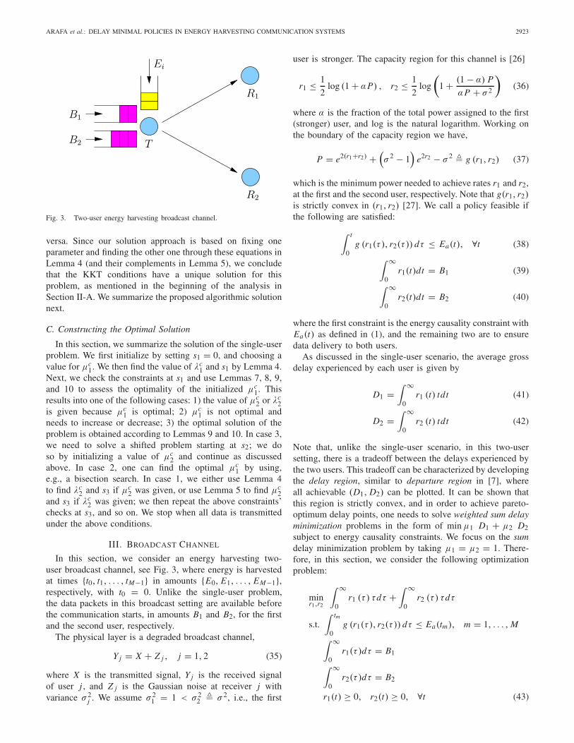
In this section, we consider an energy harvesting two-user broadcast channel, see Fig. 3, where energy is harvestedat times {t0, t1, . . . , tM−1} in amounts {E0, E1, . . . , EM−1},respectively, with t0 = 0. Unlike the single-user problem,the data packets in this broadcast setting are available beforethe communication starts, in amounts B1 and B2, for the firstand the second user, respectively.

The physical layer is a degraded broadcast channel,

Y j = X + Z j , j = 1, 2 (35)

where X is the transmitted signal, Y j is the received signalof user j , and Z j is the Gaussian noise at receiver j withvariance σ 2

j . We assume σ 21 = 1 < σ 2

2 � σ 2, i.e., the first

user is stronger. The capacity region for this channel is [26]

r1 ≤ 1

2log (1 + αP) , r2 ≤ 1

2log

(1 + (1 − α) P

αP + σ 2

)(36)

where α is the fraction of the total power assigned to the first(stronger) user, and log is the natural logarithm. Working onthe boundary of the capacity region we have,

P = e2(r1+r2) +(σ 2 − 1

)e2r2 − σ 2 � g (r1, r2) (37)

which is the minimum power needed to achieve rates r1 and r2,at the first and the second user, respectively. Note that g(r1, r2)is strictly convex in (r1, r2) [27]. We call a policy feasible ifthe following are satisfied:

∫ t

0g (r1(τ ), r2(τ )) dτ ≤ Ea(t), ∀t (38)

∫ ∞

0r1(t)dt = B1 (39)

∫ ∞

0r2(t)dt = B2 (40)

where the first constraint is the energy causality constraint withEa(t) as defined in (1), and the remaining two are to ensuredata delivery to both users.

As discussed in the single-user scenario, the average grossdelay experienced by each user is given by

D1 =∫ ∞

0r1 (t) tdt (41)

D2 =∫ ∞

0r2 (t) tdt (42)

Note that, unlike the single-user scenario, in this two-usersetting, there is a tradeoff between the delays experienced bythe two users. This tradeoff can be characterized by developingthe delay region, similar to departure region in [7], whereall achievable (D1, D2) can be plotted. It can be shown thatthis region is strictly convex, and in order to achieve pareto-optimum delay points, one needs to solve weighted sum delayminimization problems in the form of min μ1 D1 + μ2 D2subject to energy causality constraints. We focus on the sumdelay minimization problem by taking μ1 = μ2 = 1. There-fore, in this section, we consider the following optimizationproblem:

minr1,r2

∫ ∞

0r1 (τ ) τdτ +

∫ ∞

0r2 (τ ) τdτ

s.t.∫ tm

0g (r1(τ ), r2(τ )) dτ ≤ Ea(tm), m = 1, . . . , M

∫ ∞

0r1(τ )dτ = B1

∫ ∞

0r2(τ )dτ = B2

r1(t) ≥ 0, r2(t) ≥ 0, ∀t (43)


A. Minimum Sum Delay Policy

We note that (43) is a convex optimization problem [27].We solve using a Lagrangian approach:

L =∫ ∞

0r1 (τ ) τdτ +

∫ ∞

0r2 (τ ) τdτ

+M∑

m=1

λm

(∫ tm

0g (r1(τ ), r2(τ )) dτ − Ea(tm)

)

− ν1

(∫ ∞

0r1(τ )dτ − B1

)− ν2

(∫ ∞

0r2(τ )dτ − B2

)

−∫ ∞

0γ1(τ )r1(τ )dτ −

∫ ∞

0γ2(τ )r2(τ )dτ (44)

where {λm}, ν1, ν2, γ1(t), and γ2(t) are Lagrange multipliers.KKT optimality conditions are:

t + λ(t)∂g (r1(t), r2(t))

∂r1(t)− ν1 − γ1(t) = 0 (45)

t + λ(t)∂g (r1(t), r2(t))

∂r2(t)− ν2 − γ2(t) = 0 (46)

where we have:

λ(t) =∑

{m:tm≥t}λm (47)

∂g (r1(t), r2(t))

∂r1(t)= 2e2(r1(t)+r2(t)) (48)

∂g (r1(t), r2(t))

∂r2(t)= 2e2(r1(t)+r2(t)) + 2

(σ 2 − 1

)e2r2(t) (49)

along with the complementary slackness conditions:

λm

(∫ tm

0g (r1(τ ), r2(τ )) dτ − Ea(tm)

)= 0, ∀m (50)

ν1

(∫ ∞

0r1(τ )dτ − B1

)= 0, γ1(t)r1(t) = 0 ∀t (51)

ν2

(∫ ∞

0r2(τ )dτ − B2

)= 0, γ2(t)r2(t) = 0 ∀t (52)

From the above KKT conditions, we can write the rates andtotal power expressions in terms of the Lagrange multipliers.First, we write the rate expressions as:

r1(t) = 1

2log

((σ 2 − 1

)(γ1 (t) + ν1 − t)

γ2 (t) − γ1 (t) + ν2 − ν1

)(53)

r2(t) = 1

2log

(γ2 (t) − γ1 (t) + ν2 − ν1

λ (t)(σ 2 − 1

))

(54)

We now state the following result.Lemma 11: The optimal Lagrange multipliers (ν∗

1 , ν∗2 )

satisfy: ν∗1 < ν∗

2 < σ 2ν∗1 .

Proof: We show this by contradiction. Assume ν∗2 ≤ ν∗

1 .Then, by (54), the value of r2(t) is well-defined only if γ2(t) >0 ∀t , which means by complementary slackness that r2(t) =0 ∀t . Therefore, assuming B2 > 0, the weak user will neverget to receive any of its data. This proves the first inequality.

To show the second inequality, assume σ 2ν∗1 ≤ ν∗

2 . Thus,(σ 2 − 1

)(ν1 − t)

γ2 (t) + ν2 − ν1≤ 1, ∀t, γ2(t) ≥ 0 (55)

Therefore, the right hand side of (53) can only be positive ifγ1(t) > 0, but this means, by complementary slackness, thatr1(t) = 0, which is a contradiction. Hence, r1(t) = 0 ∀t , and,assuming B1 > 0, the strong user will never get to receive anyof its data.

Next, we characterize the optimal total transmit powerg (r1(t), r2(t)) by the following lemma. The proof is inAppendix G.

Lemma 12: In the optimal policy, the total transmit powerg (r1(t), r2(t)) is given by

g(r1(t), r2(t)) = max

{ν2 − t

λ(t)− σ 2,

ν1 − t

λ(t)− 1

}+(56)

The above lemma shows that the optimal power in thebroadcast channel decreases with time between energy har-vests, and can reach zero before increasing again with thenext energy harvest, similar to the results of the single-userchannel in Section II. The following lemmas characterize thestructure of the optimal policy.

Lemma 13: In the optimal policy, the transmission starts bysending data to the strong user, and finishes by sending datato the weak user.

Proof: We show this by contradiction. Assume that thetransmission starts by sending data to the weak user only,i.e., r2(0) > r1(0) = 0.4 By complementary slackness,we have γ2(0) = 0. By Lemma 11, since σ 2ν1 > ν2, we have

(σ 2 − 1

)(γ1(0) + ν1)

ν2 − ν1 − γ1(0)> 1, ∀γ1(0) ≥ 0 (57)

which implies, by (53), that r1(0) > 0, which is a contra-diction. For the second part of the lemma, assume that thetransmission ends at some time t f with r1(t f ) > r2(t f ) = 0.By Lemma 12, we know that this can only occur if λ(t f ) >ν2−ν1σ 2−1

� λth . Since λ(t) is non-increasing, we have λ(t) ≥λ(t f ), ∀t ≤ t f . This means that λ(t) does not fall below λth

throughout the transmission, which is equivalent to saying,again by Lemma 12, that the weak user does not receive anyof its data, which is a contradiction.

Lemma 14: For t < tth � σ 2ν1−ν2σ 2−1

, if the transmitter issending data, then it is sending to the strong user.

Proof: We show this by contradiction. Assume that forsome t < tth data is sent only to the weak user, i.e., wehave r1(t) = 0 and r2(t) > 0. By complementary slackness,we have γ2(t) = 0. Since t < tth , it follows by simplemanipulations that the numerator of the term inside the login (53) is strictly larger than its denominator ∀γ1(t) ≥ 0,i.e., r1(t) > 0, which is a contradiction. The only case wherer1(t) = 0 for some t < tth is when γ2(t) > 0, which meansby complementary slackness that r2(t) = 0.

1) Modes of Operation: There can be four different modesof operation at a given time, depending on which user isreceiving data. The first mode is when only the strong useris receiving data, i.e., r1(t) > 0 and r2(t) = 0. By Lemma 12,this can be the case only if λ(t) ≥ λth = ν2−ν1

σ 2−1. In this mode,

4Extension of the contradiction arguments in this lemma to an ε-lengthinterval, ε > 0, follows directly.


we have the total power and the strong user’s rate given by

g(r1(t), 0) = ν1 − t

λ(t)− 1 (58)

r1(t) = 1

2log

(ν1 − t

λ(t)

)(59)

The second mode of operation is when both users arereceiving data, i.e., r1(t) > 0 and r2(t) > 0. Again byLemma 12, this can be the case only if λ(t) < λth . Moreover,by (53), we also need t < tth = σ 2ν1−ν2

σ 2−1. In this mode, the total

power and the users’ rates are given by

g(r1(t), r2(t)) = ν2 − t

λ(t)− σ 2 (60)

r1(t) = 1

2log

((σ 2 − 1)(ν1 − t)

ν2 − ν1

)(61)

r2(t) = 1

2log

(ν2 − ν1

λ(t)(σ 2 − 1)

)(62)

The third mode of operation is when only the weak user isreceiving data, i.e., r1(t) = 0 and r2(t) > 0. For this to occurwe need both λ(t) < λth and t ≥ tth . The total power and theweak user’s rate are then given by

g(0, r2(t)) = ν2 − t

λ(t)− σ 2 (63)

r2(t) = 1

2log

(ν2 − t

λ(t)σ 2

)(64)

The fourth mode is when both rates (and the power) arezero. We denote this mode as a communication gap. Thesegaps may occur, for instance, if there is a small amount ofenergy in the battery that is insufficient to deliver all the data,and a large amount of energy arrives later. The transmittermay then finish up this small amount of energy to send somebits out and wait for additional energy to send the remainingbits.

2) Finding the Value of λ(t): We next characterize the ratesand powers. The following lemma shows that λ(t) is a piece-wise constant function. The proof follows by complementaryslackness as in the proof of Lemma 1, and is omitted forbrevity.

Lemma 15: In the optimal policy, the Lagrange multiplierfunction λ(t) is piecewise constant, with possible changes onlywhen energy is depleted.

By Lemma 15, λ(t) is a sequence rather than a continuousfunction of time. Following the same notation as in the single-user channel, we denote the times of change of λ(t) by{s1, s2, . . . , sL} with s1 = 0, and the values of λ(t) betweensuch times by

λ(t) ={

λck, t ∈ [sk, sk+1)

λcL , t ∈ [sL,∞)

(65)

Next, we characterize the optimal {λck} sequentially. Deter-

mining the value of λck requires the knowledge of ν∗

1 and ν∗2 ,

and also which mode of operation is active during the inter-val [sk, sk+1). Let us define B j (t) as the total amount of bitstransmitted to user j by time t . The next lemma shows howto compute λc

k given the mode of operation. The proof uses

similar steps as in the proof of Lemma 4 in the single-usersetting and is omitted for brevity.

Lemma 16: Given a mode of operation, with the optimalν∗

1 , ν∗2 , λc

l , sl , ∀l < k, define the following quantities ∀m:tm > sk

λ̄m : E∗(sk) +∫ tm

sk

g(r1(τ ), r2(τ ))+dτ = Ea(tm) (66)

λ̃1 : B∗1 (sk) +

∫ ∞

sk

r1(τ )+dτ = B1 (67)

λ̃2 : B∗2 (sk) +

∫ ∞

sk

r2(τ )+dτ = B2 (68)

where r1, r2, and g(r1, r2) are defined by the mode of operationin Section III-A.1, with the convention that λ̃ j = 0 whenever amode of operation has r j = 0, j = 1, 2. Then, the optimal λc

kfor this mode of operation is given by

λck = max{λ̄m , λ̃1, λ̃2}, ∀m : tm > sk (69)

The results in Lemma 16 imply that one has to knowthe mode of operation before computing the optimal valuesof the Lagrange multipliers. Note that communication gapsoccur naturally due to the (·)+ operation in these expressions.In the next section, we develop an iterative solution thatcomputes {λc

k} based on an initial assignment of the modeof operation and the values of ν1, ν2. The solution is basedon the necessary conditions stated in the previous lemmas.By Lemma 11, we know that the optimal values of ν1, ν2 lie ina cone in R

2++. We also know, by Lemmas 12 and 13, that thecommunication stops if t > ν2. Therefore, we find an upperbound on the value of ν∗

2 as follows. First, we move all ofthe energy to tM−1, the arrival time of the last energy packet,and start the communication from there. Second, we solve thissingle energy arrival problem and find its optimal ν∗

2 whichwe denote by ν

single2 . Therefore, an upper bound on ν∗

2 of themultiple energy arrival problem is

ν∗2 ≤ ν

single2 + tM−1 � νub (70)

Once this upper bound is found, one can perform a two-dimensional grid search over the feasible region of ν1, ν2:

Rν1ν2 ={ν1, ν2 : 0 < ν1 < ν2 < σ 2ν1, ν2 ≤ νub

}(71)

Next, we analyze the single energy arrival case to characterizethe upper bound on ν∗

2 .3) Single Energy Arrival: For the single energy arrival case,

we first note that there can be no communication gaps, as thiscan only increase the delay. We also note that since thereis only one value of λ, corresponding to only one energyarrival constraint, the optimal power is given by the first termin (56). If not, then the weak user will never receive its data.Hence, the first mode of operation where only the strong useris receiving data never occurs. Thus, the optimal total poweris given by

ps(t) = ν2 − t

λ− σ 2, ∀t ≤ t f � ν2 − λσ 2 (72)

where the subscript s denotes single arrival, and t f is suchthat ps(t) is non-negative. From the above, we also note that


λ cannot be 0, or else the power is infinitely large. Since λ > 0,by complementary slackness, the transmitter has to consumeall of its energy by the end of transmission. This simplifies thesingle energy arrival problem, as in this case, we have all thethree constraints, both users’ data and transmitter’s energy, metwith equality. Therefore, we can solve for the optimal valuesof the Lagrange multipliers satisfying the following:

∫ tth

0

1

2log

((σ 2 − 1)(ν1 − t)

ν2 − ν1

)dt = B1 (73)

tth

2log

(ν2 − ν1

λ(σ 2 − 1)

)+

∫ t f

tth

1

2log

(ν2 − t

λσ 2

)dt = B2 (74)

∫ t f

0ps(t)dt = E (75)

The above three equations are direct consequences of themodes of operation analysis in Section III-A.1. These can befurther simplified into:

ν1

2log

((σ 2 − 1)ν1

ν2 − ν1

)= B1 (76)

ν2

2log

(ν2 − ν1

λ(σ 2 − 1)

)= B2 (77)

(ν2 − λσ 2

)2

2λ= E (78)

Note that (76)-(78) are three equations in three unknowns, andcan be solved numerically for the values of λ∗, ν∗

1 , and ν∗2 .

Note from the above analysis that, since we always start withthe second mode of operation, where both users receive data,in this setting, we have λ < λth . This implies that t f > tth ,and enables the following stronger version of Lemma 13.

Lemma 17: In the optimal policy solving (43), transmissionalways ends by sending data only to the weak user.

Proof: In the single energy arrival case, since t f > tth ,we always end transmission by sending data only to the weakuser. In the multiple arrival case, the last energy arrival can beviewed as a single energy arrival problem with the remainingdata in the data buffers as modified constraints. Then the singleenergy arrival result applies, yielding the stated result.

We have now characterized how to get the upper bound νub

in (70). In the next section we present an iterative method tofind the optimal Lagrange multipliers solving problem (43).

B. Iterative SolutionThe analysis presented in Lemma 16 describes an optimal

method of finding {λck} given ν∗

1 and ν∗2 . To find the latter two,

we perform a grid search over the region Rν1ν2 , which is fullycharacterized by the single arrival analysis. We perform thesearch as follows. We fix (ν1, ν2) ∈ Rν1ν2 , and solve for {λc

k}to acquire a transmission policy accordingly. We denote byMode 1, Mode 2, and Mode 3, the mode of operation wheredata is sent only to the strong user, both users, and only to theweak user, respectively. Since Mode 1 can only occur at thebeginning, we assume that the transmission starts according tothat mode, and compute the corresponding λs by Lemma 16.If these λs are all less than λth , then they are correct. We moveto Mode 2 once we get a value of λ larger than λth . We stay at

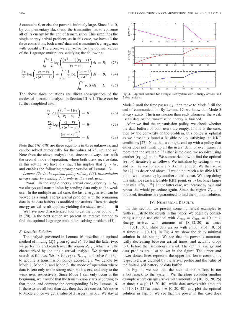
Fig. 4. Optimal solution for a single-user system with 3 energy arrivals and2 data arrivals.

Mode 2 until the time passes tth , then move to Mode 3 till theend of communication. By Lemma 17, we know that Mode 3always exists. The transmission then ends whenever the weakuser’s data or the transmission energy is finished.

After we find the transmission policy, we check whetherthe data buffers of both users are empty. If this is the case,then by the convexity of the problem, this policy is optimalas we have thus found a feasible policy satisfying the KKTconditions [27]. Note that we might end up with a policy thateither does not finish up all the users’ data, or even transmitsmore than the available. If either is the case, we re-solve usinganother (ν1, ν2) point. We summarize how to find the optimal(ν1, ν2) iteratively as follows. We initialize by setting ν1 = εand ν2 = ν1 + ε for some ε > 0 small enough. We then solvefor {λc

k} as described above. If we do not reach a feasible KKTpoint, we increase ν2 by another ε and repeat. We keep doingthis until we reach a feasible KKT point, or ν2 becomes largerthan min{σ 2ν1, ν

ub}. In the latter case, we increase ν1 by ε andrepeat the whole procedure again. Since the region Rν1ν2 isbounded, iterations are guaranteed to find the optimal solution.

IV. NUMERICAL RESULTS

In this section, we present some numerical examples tofurther illustrate the results in this paper. We begin by consid-ering a single use channel with Emax = Bmax = 10 units.Energy arrives with amounts of [8, 12, 20] at timest = [0, 10, 30], while data arrives with amounts of [10, 15]at times t = [0, 10]. In Fig. 4 we show the delay minimalsolution in this setting. We see that the power is monoton-ically decreasing between arrival times, and actually dropsto 0 before the last energy arrival. The optimal energy anddata profiles are also shown in the figure. The upper andlower dotted lines represent the upper and lower constraints,respectively, as dictated by the arrival profile and the value ofthe finite-sized battery or data buffer.

In Fig. 4, we see that the size of the buffers is nota bottleneck to the system. We therefore consider anotherexample where energy arrives with amounts of [10, 15, 20, 25]at times t = [0, 15, 20, 40], while data arrives with amountsof [10, 18, 22] at times t = [0, 20, 40], and plot the optimalsolution in Fig. 5. We see that the power in this case does


Fig. 5. Effects of having a finite-sized battery and data buffer in a single-usersystem.

Fig. 6. Optimal power and rates for a system with four energy arrivals.

not drop down to 0 until at the end of communication,and that its slope changes when the optimal energy or dataprofiles hit the lower bounds indicated by the size of thebuffers.

Next, we present a numerical example to illustrate theresults of the broadcast setting. We consider a systemwhere energy arrives with values [6, 10, 4, 5] at times t =[0, 70, 100, 150], with amounts of data B1 = 8 and B2 = 4.25intended for the strong and the weak user, respectively. We firstfind the upper bound on ν∗

2 by solving the single energy arrivalcase by setting E = 25 in (78) and finding the value of ν

single2 .

Adding tM−1 = 150, we get νub 170. We then apply theiterative solution described in Section III-B to find the optimaltotal power allocation for the multiple arrival case and thecorresponding users’ rates. These are shown in Fig. 6 as afunction of time. We see that all four modes of operation arepresent in this example: the transmitter begins by sending dataonly to the strong user (Mode 1) until it consumes the initialenergy arrival, and stays silent until the next energy arrival,then it sends data to both users simultaneously (Mode 2) untilall strong user’s data is finished, which occurs at tth 79.4.Then, it starts sending data only to the weak user (Mode 3),before keeping silent until the third energy arrival, and thenfinishes up the weak user’s data. Note that the fourth energy

Fig. 7. Optimal energy and data consumption.

arrival is not used in this example. In Fig. 7, we show thecorresponding optimal total energy and data consumption forthis policy as a function of time.

Finally, we compare this to the transmission completiontime minimization problem in [7] with the same data valuesand energy arrival profile. The optimal transmission com-pletion time is equal to T ∗ = 90. Calculating the delayachieved by such policy gives D 717.2. On the otherhand, our delay minimizing policy achieves a smaller delay ofD∗ 593.3, however, it takes a larger amount of time to finishT 101.5. This shows that there exists a tradeoff betweendelay minimization and transmission completion time mini-mization, and that the two problems are different, even whenall data is available before the start of communication. That is,finishing data delivery by a minimum time, and having dataexperience minimum overall delay yield different optimumpolicies.

V. CONCLUSION AND DISCUSSION

We considered delay minimization in energy harvestingcommunication channels. First, we studied the single-userchannel where the transmitter has a finite-sized battery anddata buffer, and energy and data packets become available atthe transmitter during the course of communication. We deter-mined the optimum power control policy in terms of theLagrange multiplier functions. We identified the propertiesof these functions and gave a method that evaluates themrecursively. We proposed a solution which iteratively updatesthe initial value of a Lagrange multiplier, and obtains theoptimum power allocation policy. The optimal power valuesstart high, decrease linearly, potentially reaching zero betweenenergy harvests and data arrivals. This policy is different fromthe piecewise constant power policies of the existing literaturewhich focus on minimizing a deadline by which all packetsare transmitted or maximizing the throughput before a fixeddeadline. Initial high powers in our case make sure that thedelay does not accumulate by transmitting data at faster ratesfirst, then decreasing the rate gradually.

Next, we considered a two-user energy harvesting broadcastchannel and characterized the minimal sum delay policysubject to energy harvesting constraints, when the transmitterhas an infinite-sized battery, and all data intended for both


users is available before transmission. We showed that theoptimal power is decreasing between energy harvests, and thatthere can be times when data is sent only to the strong user,both users, or only to the weak user. We also showed that therecan be communication gaps where the transmitter is silentbetween energy arrivals. We presented a method to find theoptimal policy iteratively.

We note that there is another metric that is considered incurrent energy harvesting literature that resembles delay in cer-tain aspects. That is, the age of information metric [28]–[37].This metric measures the delay from the receiver’s perspec-tive, and is defined as the time spent since the freshestinformation packet has been received by the receiver. In ourrecent work [32], we have discussed the precise difference,mathematically, between delay and age minimization problemsin energy harvesting systems; see [32, Sec. V]. In summary,the main difference lies in that the age metric is more sensitiveto data packets’ arrival times than the delay metric (which ismainly due to the difference in definitions of both metrics), andhence the solutions of both problems can be much different.It is therefore of interest to study the problems in this paperunder an age metric and relate the solutions of these two linesof research.

APPENDIX

A. Necessity of KKT Conditions of Optimalityfor Problem (9)

It is known that the (extended) Fritz John conditions foroptimality [38] are always necessary. If we apply such con-ditions for our problem, we get that any optimal solutionshould be a stationary point of a slightly modified Lagrangiancompared to L in (10) where an extra Lagrange multiplierκ ≥ 0 is multiplied by the objective function. We notethat the Fritz John conditions are weaker than the KKTconditions since the optimal κ∗ may turn out to be 0, andhence the objective function vanishes from the Lagrangian atthe optimal solution. We also note that the KKT conditionswill be directly implied if one can show that κ∗ > 0, sinceone can divide all other Lagrange multipliers by κ∗ in this caseafter differentiating and equating to 0, and hence any optimalsolution would be a stationary point of the Lagrangian in (10)in this case, i.e., with κ = 1. We show that κ∗ > 0 by thefollowing contradiction argument.

Assume that κ∗ = 0. Then, the optimal p(t) should satisfy

p(t) =(

μ(t)

λ(t)− 1

)+

which means, by Lemma 1, that in any optimal solution,the power policy is a piece wise constant function. Now chooseany interval (l1, l2) over which p(t) = l for some constantl > 0. Using arguments similar to those in Lemma 3, we candefine another policy p′(t) to be monotonically decreasingon (l1, l2), consuming the same amount of energy, deliveringthe same amount of data, and achieving strictly less delay.Since this monotonically decreasing policy can only be satis-fied if and only if κ∗ > 0, and is better than any other policywith κ∗ = 0, then the assumption of κ∗ = 0 cannot be true,and KKT conditions are necessary for optimality.

B. Proof of Lemma 6

Assume without loss of generality that Ei (s) = Bi (s) = 0,for i = 0, 1, 2. Since we have E1(s̄) = E0(s̄), and thatp1(t) declines slower than p0(t), therefore it must hold thatE0(t) = ∫ t

s p0(τ )dτ ≥ ∫ ts p1(τ )dτ = E1(t) ∀t ∈ [s, s̄],

i.e., p0(t) majorizes p1(t) in the interval [s, s̄]. By concavity ofthe log, it then follows that B1(s̄) = ∫ s̄

s12 log(1 + p1(t))dt >

∫ s̄s

12 log(1 + p0(t))dt = B0(s̄) by the theory of continuous

majorization [39]. This proves the first part of the lemma.We prove the second part by contradiction. Assume E2(s̄) ≥

E0(s̄). Since p2(t) declines slower than p0(t), therefore theremust exist some point t ′ ∈ (s, s̄] at which E2(t ′) = E0(t ′)with E0(t) ≥ E2(t) ∀t ∈ [s, t ′]. Using the first assertion ofthe lemma, we have

B2(t′) > B0(t

′) (79)

Since E2(s̄) ≥ E0(s̄), then we must have

B2(s̄) − B2(t′) > B0(s̄) − B0(t

′) (80)

From (79) and (80), we get B2(s̄) > B0(s̄), which contradictsthe assumption that both policies depart the same amount ofdata. Therefore we must have E2(s̄) < E0(s̄).

C. Proof of Lemma 7By complementary slackness, we know that we must have

μck+1 = μc

k since the data constraints are not binding at sk+1.However, if μc

k ≤ sk+1, then by (11), p(t) = 0 ∀t ≥ sk+1,and the transmitter will not be able to deliver the requiredamount of data to the receiver. Hence, μc

k needs to increase inorder to maintain feasibility of the problem. This proves thefirst part of the lemma. To show the second part, we also notethat by complementary slackness, we must have λc

k+1 = λck

since the energy constraints are not binding at sk+1. However,if sk+1 = ∞, i.e., we reached the end of the communicationsession, then we can use some extra amounts of energy todecrease the delay as follows: decrease the value of μc

k anddecrease that of λc

k such that the amounts of departed bits in[sk,∞) stays the same. This makes the power in the interval[sk,∞) be of a faster decline, i.e., finish transmission faster,and in turn by Lemma 6 will consume more energy, which isfeasible since the energy constraints are not binding.

D. Proof of Lemma 8To show the first part, let us increase the value of μc

kand increase that of λc

k such that the consumed energy inthe interval [sk, sk+1) stays the same. This means that thepower in the interval [sk, sk+1) will have a slower decline.By Lemma 6, this new policy departs more bits, and preventsthe overflow of the data buffer. Similarly, for the second part,let us decrease the value of μc

k and decrease that of λck such

that the data delivered in the interval [sk, sk+1) stays the same.This means that the power in the interval [sk, sk+1) will havea faster decline, and in turn by Lemma 6 will consume moreenergy and prevent the overflow of the battery.

E. Proof of Lemma 9We first note that the conditions of optimality stated in the

lemma are those stated in Lemma 2. If these are not satisfied,


and the battery is empty while the data buffer is full at sk+1,then we can increase the value of μc

k and increase that of λck

such that the consumed energy in [sk, sk+1) stays the same.This means that the power in the interval [sk, sk+1) will havea slower decline. By Lemma 6, this new policy departs morebits, which is feasible since the data buffer is full at sk+1, andeventually achieves less delay. The proof of the other scenariostated in the lemma where the battery is full and the databuffer is empty at sk+1 follows using similar arguments as inthe proof of the second part of Lemma 8.

F. Proof of Lemma 10We first note that the conditions of optimality stated in the

lemma are those stated in Lemma 2. If these are not satisfied,and both the battery and the data buffer are empty at sk+1,and λ̄k+1 > λc

k , then we can increase the value of μck and

increase that of λck such that the amount of data delivered

in [sk, sk+1) stays the same. This means that the power in theinterval [sk, sk+1) will have a slower decline. By Lemma 6, thisnew policy consumes a smaller amount of energy, i.e., energyconstraints will not be binding at sk+1, and therefore we willhave λc

k+1 = λck . On the other hand if μ̄k+1 < μc

k , then wecan decrease the value of μc

k and decrease that of λck such

that the amount of energy consumed in [sk, sk+1) stays thesame. This means that the power in the interval [sk, sk+1) willhave a faster decline. By Lemma 6, this new policy deliversa smaller amount of data, i.e., data constraints will not bebinding at sk+1, and therefore we will have μc

k+1 = μck . The

proof of the other scenario stated in the lemma where boththe battery and the data buffer are full follows using similararguments.

G. Proof of Lemma 12From (46) and (49), we have

g(r1(t), r2(t)) = ν2 + γ2(t) − t

λ(t)− σ 2 (81)

Since from (48) and (49) we always have

∂g(r1(t), r2(t))

∂r2(t)− σ 2 ≥ ∂g(r1(t), r2(t))

∂r1(t)− 1 (82)

with equality iff r2(t) = 0, from (45) and (46), we have

ν2 + γ2(t) − t

λ(t)− σ 2 ≥ ν1 + γ1(t) − t

λ(t)− 1 (83)

Thus, if r2(t) > 0, by complementary slackness γ2(t) = 0,and the total power is given by

g(r1(t), r2(t)) = ν2 − t

λ(t)− σ 2 (84)

>ν1 + γ1(t) − t

λ(t)− 1 (85)

≥ ν1 − t

λ(t)− 1 (86)

On the other hand, if r2(t) = 0 and r1(t) > 0, we have

g(r1(t), r2(t)) = ν2 + γ2(t) − t

λ(t)− σ 2 (87)

= ν1 − t

λ(t)− 1 (88)

≥ ν2 − t

λ(t)− σ 2 (89)

Finally, if both rates are zero, then the total power is zero.Combining this with the above gives (56).

REFERENCES

[1] T. Tong, S. Ulukus, and W. Chen, “Optimal packet scheduling for delayminimization in an energy harvesting system,” in Proc. IEEE ICC,Jun. 2015, pp. 4241–4246.

[2] M. Fu, A. Arafa, S. Ulukus, and W. Chen, “Delay minimal policies inenergy harvesting broadcast channels,” in Proc. IEEE ICC, May 2016,pp. 1–6.

[3] J. Yang and S. Ulukus, “Optimal packet scheduling in an energy har-vesting communication system,” IEEE Trans. Commun., vol. 60, no. 1,pp. 220–230, Jan. 2012.

[4] K. Tutuncuoglu and A. Yener, “Optimum transmission policies for bat-tery limited energy harvesting nodes,” IEEE Trans. Wireless Commun.,vol. 11, no. 3, pp. 1180–1189, Mar. 2012.

[5] O. Ozel, K. Tutuncuoglu, J. Yang, S. Ulukus, and A. Yener, “Transmis-sion with energy harvesting nodes in fading wireless channels: Optimalpolicies,” IEEE J. Sel. Areas Commun., vol. 29, no. 8, pp. 1732–1743,Sep. 2011.

[6] C. K. Ho and R. Zhang, “Optimal energy allocation for wirelesscommunications with energy harvesting constraints,” IEEE Trans. SignalProcess., vol. 60, no. 9, pp. 4808–4818, Sep. 2012.

[7] J. Yang, O. Ozel, and S. Ulukus, “Broadcasting with an energy harvest-ing rechargeable transmitter,” IEEE Trans. Wireless Commun., vol. 11,no. 2, pp. 571–583, Feb. 2012.

[8] M. A. Antepli, E. Uysal-Biyikoglu, and H. Erkal, “Optimal packetscheduling on an energy harvesting broadcast link,” IEEE J. Sel. AreasCommun., vol. 29, no. 8, pp. 1721–1731, Sep. 2011.

[9] O. Ozel, J. Yang, and S. Ulukus, “Optimal broadcast scheduling foran energy harvesting rechargebale transmitter with a finite capacitybattery,” IEEE Trans. Wireless Commun., vol. 11, no. 6, pp. 2193–2203,Jun. 2012.

[10] J. Yang and S. Ulukus, “Optimal packet scheduling in a multiple accesschannel with energy harvesting transmitters,” J. Commun. Netw., vol. 14,no. 2, pp. 140–150, Apr. 2012.

[11] K. Tutuncuoglu and A. Yener, “Sum-rate optimal power policies forenergy harvesting transmitters in an interference channel,” J. Commun.Netw., vol. 14, no. 2, pp. 151–161, Apr. 2012.

[12] C. Huang, R. Zhang, and S. Cui, “Throughput maximization for theGaussian relay channel with energy harvesting constraints,” IEEE J. Sel.Areas Commun., vol. 31, no. 8, pp. 1469–1479, Aug. 2013.

[13] D. Gündüz and B. Devillers, “Two-hop communication with energyharvesting,” in Proc. IEEE CAMSAP, Dec. 2011, pp. 201–204.

[14] O. Orhan and E. Erkip, “Optimal transmission policies for energyharvesting two-hop networks,” in Proc. CISS, Mar. 2012, pp. 1–6.

[15] Y. Luo, J. Zhang, and K. B. Letaief, “Optimal scheduling and powerallocation for two-hop energy harvesting communication systems,” IEEETrans. Wireless Commun., vol. 12, no. 9, pp. 4729–4741, Sep. 2013.

[16] B. Gurakan, O. Ozel, J. Yang, and S. Ulukus, “Energy cooperation inenergy harvesting communications,” IEEE Trans. Commun., vol. 61,no. 12, pp. 4884–4898, Dec. 2013.

[17] D. Gündüz and B. Devillers, “A general framework for the optimizationof energy harvesting communication systems with battery imperfec-tions,” J. Commun. Netw., vol. 14, no. 2, pp. 130–139, Apr. 2012.

[18] K. Tutuncuoglu, A. Yener, and S. Ulukus, “Optimum policies foran energy harvesting transmitter under energy storage losses,” IEEEJ. Select. Areas Commun., vol. 33, no. 3, pp. 476–481, Mar. 2015.

[19] O. Ozel, K. Shahzad, and S. Ulukus, “Optimal energy allocation forenergy harvesting transmitters with hybrid energy storage and processingcost,” IEEE Trans. Signal Process., vol. 62, no. 12, pp. 3232–3245,Jun. 2014.

[20] O. Orhan, D. Gunduz, and E. Erkip, “Throughput maximization for anenergy harvesting communication system with processing cost,” in Proc.IEEE ITW, Sep. 2012, pp. 84–88.

[21] J. Xu and R. Zhang, “Throughput optimal policies for energy harvestingwireless transmitters with non-ideal circuit power,” IEEE J. Sel. AreasCommun., vol. 32, no. 2, pp. 322–332, Feb. 2014.


[22] A. Arafa and S. Ulukus, “Optimal policies for wireless networks withenergy harvesting transmitters and receivers: Effects of decoding costs,”IEEE Sel. Areas Commun., vol. 33, no. 12, pp. 2611–2625, Dec. 2015.

[23] A. Arafa, A. Baknina, and S. Ulukus, “Energy harvesting two-waychannels with decoding and processing costs,” IEEE Trans. GreenCommun. Netw., vol. 1, no. 1, pp. 3–16, Mar. 2017.

[24] J. Yang and S. Ulukus, “Delay-minimal transmission for energy con-strained wireless communications,” in Proc. IEEE ICC, May 2008,pp. 3531–3535.

[25] D. G. Luenberger, Optimization by Vector Space Methods. Hoboken, NJ,USA: Wiley, 1997.

[26] T. M. Cover and J. A. Thomas, Elements of Information Theory.Hoboken, NJ, USA: Wiley, 2006.

[27] S. P. Boyd and L. Vandenberghe, Convex Optimization. Cambridge,U.K.: Cambridge Univ. Press, 2004.

[28] B. T. Bacinoglu, E. T. Ceran, and E. Uysal-Biyikoglu, “Age of informa-tion under energy replenishment constraints,” in Proc. ITA, Feb. 2015,pp. 25–31.

[29] R. D. Yates, “Lazy is timely: Status updates by an energy harvestingsource,” in Proc. IEEE ISIT, Jun. 2015, pp. 3008–3012.

[30] X. Wu, J. Yang, and J. Wu, “Optimal status update for age of informationminimization with an energy harvesting source,” IEEE Trans. GreenCommun. Netw., to be published.

[31] B. T. Bacinoglu and E. Uysal-Biyikoglu, “Scheduling status updates tominimize age of information with an energy harvesting sensor,” in Proc.IEEE ISIT, Jun. 2017, pp. 1122–1126.

[32] A. Arafa and S. Ulukus, “Age minimization in energy harvesting com-munications: Energy-controlled delays,” in Proc. Asilomar, Oct. 2017.

[33] A. Arafa and S. Ulukus, “Age-minimal transmission in energy harvestingtwo-hop networks,” in Proc. IEEE Globecom, Dec. 2017, pp. 1–6.

[34] A. Arafa, J. Yang, S. Ulukus, and H. V. Poor, “Age-minimal online poli-cies for energy harvesting sensors with incremental battery recharges,”in Proc. ITA, Feb. 2018.

[35] A. Arafa, J. Yang, and S. Ulukus, “Age-minimal online policies forenergy harvesting sensors with random battery recharges,” in Proc. IEEEICC, May 2018.

[36] A. Baknina, O. Ozel, J. Yang, S. Ulukus, and A. Yener. (2017).“Sending information through status updates.” [Online]. Available:https://arxiv.org/abs/1801.04907

[37] A. Baknina and S. Ulukus, “Coded status updates in an energy harvestingerasure channel,” in Proc. CISS, Mar. 2018.

[38] O. L. Mangasarian and S. Fromovitz, “The Fritz John necessary opti-mality conditions in the presence of equality and inequality constraints,”J. Math. Anal. Appl., vol. 17, no. 1, pp. 37–47, 1967.

[39] A. W. Marshall, I. Olkin, and B. C. Arnold, Inequalities: Theory ofMajorization and Its Applications. New York, NY, USA: Springer, 2011.

Ahmed Arafa (S’13–M’17) received the B.Sc.degree (Hons.) in electrical engineering fromAlexandria University, Egypt, in 2010, the M.Sc.degree in wireless technologies from the WirelessIntelligent Networks Center, Nile University, Egypt,in 2012, the M.Sc. degree in electrical engineer-ing from the University of Maryland in 2016, andthe Ph.D. degree in electrical engineering from theUniversity of Maryland at College Park in 2017.He was a Distinguished Dissertation Fellow at theDepartment of Electrical and Computer Engineering,

University of Maryland at College Park, for his Ph.D. thesis on the designand analysis of optimal communication networks with system costs.

In 2017, he joined the Electrical Engineering Department, Princeton Uni-versity, as a Post-Doctoral Research Associate. His research interests are inwireless communications, information theory, and optimization.

Tian Tong received the B.S. degree in electronicengineering from Tsinghua University in 2015.He is currently pursuing the Ph.D. degree withthe Department of Electrical and Computer Engi-neering, Carnegie Mellon University. His researchinterests include the information and network theo-retical aspects of energy harvesting communicationsystems.

Minghan Fu received the B.S. degree in EE fromTsinghua University in 2016 and the master’s degreefrom the CMU CS Department, with a focus on dis-tributed systems. Since 2015, she has been exploringthe possibility of using reusable energy for efficientcommunications. She is currently with Snap Inc.,as a full-time Software Engineer, aiming at boostingthe performance for large-scale systems.

Sennur Ulukus (S’90–M’98–SM’15–F’16) receivedthe B.S. and M.S. degrees in electrical andelectronics engineering from Bilkent University, andthe Ph.D. degree in electrical and computer engineer-ing from the Wireless Information Network Labora-tory, Rutgers University. She was a Senior TechnicalStaff Member at AT&T Labs-Research. She iscurrently a Professor of electrical and computerengineering with the University of Maryland atCollege Park, where she also holds a joint appoint-ment with the Institute for Systems Research (ISR).

Her research interests are in wireless communications, information theory,signal processing, and networks, with recent focus on information theoreticphysical-layer security, private information retrieval, energy harvesting com-munications, and wireless energy and information transfer.

She is a Distinguished Scholar-Teacher of the University of Maryland. Shereceived the 2003 IEEE Marconi Prize Paper Award in wireless communi-cations, the 2005 NSF CAREER Award, the 2010–2011 ISR OutstandingSystems Engineering Faculty Award, and the 2012 ECE George CorcoranEducation Award. She was a general TPC Co-Chair of 2017 IEEE ISIT,2016 IEEE GLOBECOM, 2014 IEEE PIMRC, and 2011 IEEE CTW. Shewas an Editor of the the IEEE TRANSACTIONS ON COMMUNICATIONS

from 2003 to 2007, the IEEE TRANSACTIONS ON INFORMATION THE-ORY from 2007 to 2010, and the IEEE JOURNAL ON SELECTED AREAS

IN COMMUNICATIONS–Series on Green Communications and Networkingfrom 2015 to 2016. She was a Guest Editor of the IEEE TRANSACTIONS

ON INFORMATION THEORY in 2011, the Journal of Communications andNetworks in 2012, and the IEEE JOURNAL ON SELECTED AREAS IN COM-MUNICATIONS in 2015 and 2008. She has been on the Editorial Board of theIEEE TRANSACTIONS ON GREEN COMMUNICATIONS AND NETWORKINGsince 2016.

Wei Chen (S’05–M’07–SM’13) received the B.S.and Ph.D. degrees (Hons.) from Tsinghua Univer-sity in 2002 and 2007, respectively. From 2005 to2007, he was a Visiting Ph.D. Student with TheHong Kong University of Science and Technology.Since 2007, he has been on the faculty of TsinghuaUniversity, where he is currently a tenured Full Pro-fessor, the Director of the Academic Degree Office,Tsinghua University, and a member of the UniversityCouncil. From 2014 to 2016, he served as a DeputyHead of the Department of Electronic Engineering.

He has also held visiting appointments at several other universities. Hisresearch interests include wireless networks and information theory.

He is a member of the National 10000-Talent Program, a Cheung KongYoung Scholar, and a Chief Scientist of the National 973 Youth Project.He has been supported by the NSFC Excellent Young Investigator Project,the New Century Talent Program of the Ministry of Education, and the BeijingNova Program. He received the first prize of the 14th Henry Fok Ying-TungYoung Faculty Award, the 17th Yi-Sheng Mao Science and Technology Awardfor Beijing Youth, the 2017 Young Scientist Award of the China Instituteof Communications, and the 2015 Information Theory New Star Award ofthe China Institute of Electronics. He received the IEEE Marconi PrizePaper Award in 2009 and the IEEE Comsoc Asia Pacific Board Best YoungResearcher Award in 2011. He received the National May 1st Medal and theBeijing Youth May 4th Medal. He also serves as the Executive Chairman ofthe Youth Forum of the China Institute of Communications. He serves as anEditor for the IEEE TRANSACTIONS ON COMMUNICATIONS and the IEEETRANSACTIONS ON EDUCATION.

Documents

Delay Minimal Policies in Energy Harvesting …ulukus/papers/journal/delay-min-eh.pdf · ARAFA et al.: DELAY MINIMAL POLICIES IN ENERGY HARVESTING COMMUNICATION SYSTEMS 2923 Fig