Embed Size (px)
Citation preview

rljkswaterstaatdienst gatiidewatereab l b l i t h k 3 l C
Application-oriented validation of across-shore sediment transport model
UNIBEST-TC vs, Egmond-data
Ad J.H.M. Renters
delft hydraulics

Application-oriented validation of a cross-shore sediment transport model H 840 — June 1393
Contents
List of tablesList of figuresList of symbols
1 Introduction
2 Measurement data 22.1 Introduction 22.2 Instruments 22.3 Measuring points 3
3 Validation of measurement data 43.1 Introduction 43.2 Hydraulic measurement data 4
3.2.1 Wavec 43.2.2 Pole 3 53.2.3 Frame 73.2.4 Pole 2 83.2.5 Pole 1 9
3.3 Morphological measurement data 103.3.1 Hydrographic surveys 103.3.2 SAP-profiles 11
4 Measurement data 124.1 Introduction 12
4.2.1 Criteria for hydrodynamic validation 124.2.2 Selection of data for hydrodynamic validation 134.3.1 Criteria for morphodynamic validation 144.3.2 Selection of data for morphodynamic validation 15
5 Model description 165.1 Introduction 165.2 Hydrodynamics 165.3 Morphodynamics 20
6 Processing measurement data 216.1 Introduction 216.2 Correction of velocity measurement data 216.3 Input data UNIBESTTC computations 22
6.3.1 Incident wave field 236.3.2 Water level 246.3.3 Tidal current 24
j 6.3.4 Bottom profiles 256.3.5 Parameter settings 25
i 6.3.6 Grid size 266.4 Processing hydraulic measurement data 27
delft hydraulics
Application-oriented validation of a cross-shore sediment transport model H 840 - June 1993
(continued)
7 Validation model output data 307.1 Introduction 307.2 Hydraulic validation 30
7.2.1 Wave height 307.2.2 Incident wave angle 317.2.3 Return flow 327.2.4 Longshore velocity 327.2.5 Even velocity moments 337.2.6 Odd velocity moments 33
7.3 Morphodynamic validation 357.3.1 Profile development 357.3.2 Sediment transport rates 36
8 Conclusions and recommendations 388.1 Field data 38
8.2 Model data 39
References
Figures
Appendix A: Third-order odd velocity constituents
delft hydraulics

Application-oriented validation of a cross-shore sediment transport model H 840 — June 1993
List of tables
3.3.1 Dates hydrographic surveys3.3.2 SAP measurements
4.2.1 Run identification hydrodynamic computations Validation of UNIBESTTC
4.3.1 Combined bottom profiles
6.3.1 Bottom samples near beach pole 395006.3.2 7 as function of incident waves6.3.3 7 used in each model computation
delft hydraulics

Application-oriented validation of a cross-shore sediment transport model H 840 — June 1993
List of figures
2.1.1 Bathymetry Egmond aan Zee, 13-09-19912.1.2 Bathymetry Egmond aan Zee, 29-10-19912.3.1 General layout measuring points along coast normal
3.2.1 Significant wave height, WAVEC3.2.2 Peak wave period, WAVEC
3.2.3 Wave direction w.r.t. North, WAVEC
3.2.4 Surface elevation and current velocities, pole 3, 00 h, 16-10-19913.2.5 Energy density spectrum, pole 3, EMS-x, 00 h, 16-10-19913.2.6 Energy density spectrum, pole 3, EMS-y, 00 h, 16-10-1991
3.2.7 Surface elevation and orbital velocities, frame, 00 h, 16-10-19913.2.8 Statistical distribution of trough-crest values, pole 3, 00 h, 16-10-1991, CAP3.2.9 Statistical distribution of trough-crest values, pole 3, 00 h, 16-10-1991, PG3.2.10 Statistical distribution of trough-crest values, frame, 00 h, 16-10-1991, S43.2.11 Water level 16th and 19* October 19913.2.12 Surface elevation and current velocities, pole 2, 15 h 19-10-19913.2.13 Energy density spectrum, pole 2, 15 h 19-10-1991, CAP3.2.14 Energy density spectrum, pole 2, 15 h 19-10-1991, EMS-X
3.2.15 Energy density spectrum, pole 2, 15 h 19-10-1991, EMS-y3.2.16 Correlation diagram, pole 2, velocities November 19913.2.17 Cross section measuring lay-out EMS at poles
3.3.1 Echo soundings, line 395003.3.2 SAP-bottom profiles, line 395003.3.3 SAP-bottom profiles, line 395003.3.4 SAP-bottom profiles, line 395003.3.5 SAP-bottom profiles, line 39500
4.3.1 Non-uniqueness of the sediment transport field as derived from topographic changesonly (from de Vriend et al, 1987)
5.1.1 Flow diagram UNiBESTjrc-model
6.2.1 Surface elevation and depeaked velocities, pole 3, 00 h 16-10-19916.2.2 Surface elevation and depeaked and low-pass filtered velocities, pole 3, 00 h,
16-10-19916.2.3 Energy density spectrum, pole 3, CAP, 00 h, 16-10-19916.2.4 Energy density spectrum after correction, pole 3, EMS-X, 00 h, 16-10-19916.2.5 Energy density spectrum after correction, pole 3, EMS-y, 00 h, 16-10-19916.2.6 Surface elevation and depeaked velocities, pole 2, 15 h, 19-10-19916.2.7 Energy density spectrum after correction, pole 2, EMS-x, 15 h, 19-10-19916.2.8 Energy density spectrum after correction, pole 2, EMS-y, 15 h, 19-10-19916.2.9 Current velocities, pole 3 and frame, 17 h 15-10 to 21 h 16-10-19916.2.10 Correlation diagram velocities, velocities 16-10-1991
delft hydraulics I V

Application-oriented validation of a cross-shore sediment transport model H 840 - June 1993
LlSt Of f igures (continued)
6.3.1 Hmi, Tp, direction w.r.t. coast normal, wavec, run id: hi6.3.2 Ems, Tp, direction w.r.t. coast normal, wavec, run id: h26.3.3 H ^ , Tp, direction w.r.t. coast normal, wavec, run id: ml6.3.4 H^,, Tp, direction w.r.t. coast normal, wavec, run id; m26.3.5 H ^ , Tp, direction w.r.t. coast normal, wavec, run id: m36.3.6 Water level and tidal current velocity, run id: h i , h236.3.7 Water level and tidal current velocity, run id: ml, m2, m36.3.8 Combined bottom profiles, line 395006.3.9 Combined bottom profiles, line 395006.4.1 Flow diagram data processing6.4.2 Definition velocities and mean wave direction
7.2.1 H™, 16-10-19917.2.2 H™, 19-10-19917.2.3 Wave direction w.r.t. c.n., 16-10-19917.2.4 Wave direction w.r.t. c.n., 19-10-19917.2.5 Return velocity, 16-10-19917.2.6 Return velocity, 19-10-19917.2.7 Longshore velocity, 16-10-19917.2.8 Longshore velocity, 19-10-19917.2.9 GU2 velocity moment, 16-10-19917.2.10 GU2 velocity moment, 19-10-19917.2.11 GU3 velocity moment, 16-10-199127.2.12 GU3 velocity moment, 19-10-19917.2.13 GUS velocity moment, 16-10-19917.2.14 GU5 velocity moment, 19-10-19917.2.15 GU2UX velocity moment, 16-10-19917.2.16 GU2UX velocity moment, 19-10-19917.2.17 GU2UY velocity moment, 16-10-19917.2.18 GU2UY velocity moment, 19-10-19917.2.19 Short wave interaction, 16-10-19917.2.20 Short wave interaction, 19-10-19917.2.21 Short wave interaction, 16-10-19917.2.22 Short wave interaction, 19-10-19917.2.23 Short-long wave interaction, 16-10-19917.2.24 Short-long wave interaction, 19-10-19917.2.25 Short-long wave interaction, 16-10-19917.2.26 Short-long wave interaction, 19-10-19917.2.27 Wave-current interaction, 16-10-19917.2.28 Wave-current interaction, 19-10-19917.2.29 Wave-current interaction, 16-10-19917.2.30 Wave-current interaction, 19-10-19917.2.31 Current interaction, 16-10-19917.2.32 Current interaction, 19-10-19917.2.33 Current interaction, 16-10-19917.2.34 Current interaction, 19-10-1991
delft hydraulics

Application-oriented validation of a cross-shore sedimam transport model H 840 — June 1993
List Of f igures (continued)
7.3.1 Profile development, run id: ml7.3.2 Profile development, run id: m27.3.3 Profile development, run id: m27.3.4 Profile development, run id: m3
7.3.5 Sediment transport rates, run id: m27.3.6 Profile development, run id: m2s7.3.7 Profile development, run id: m2s
delft hydraulics Vf

Application-oriented validation of a cross-shore sediment transport model H 840 — June 1993
List of symbols
Wave propagation
EPgHnrsCg
kVDf
Db
Qb
Hm
QD50
the wave energydensity of watergravitational accelarationroot mean square wave heightgroup velocityrelative wave frequencywavenumber in direction of propagationalongshore directed depth-averaged velocitywave energy dissipation due to bottom frictionwave energy dissipation due to wave breakingfraction of breaking wavesmaximum wave heightfriction factor50% grain diameter
Longshore momentum equation
iy the longshore water-level gradient due to the tideA calibration coefficientfB friction factor due to steady currenttj\a amplitude of the orbital velocity for ! !„ ,rkls bottom roughness
Return flow
vf eddy viscosity&b near bottom oscillatory velocity amplitudeh water depthc wave phase speedD turbulent dissipationU secondary currentfi, w orbital wave velocities< z s > wave averaged surface elevationm mass flux due to breaking waves
Turbulence model
p^ coefficient of order onePd coefficient of order oneks depth mean time averaged turbulent kinetic energy
delft hydraulics VII

Application-oriented validation of a cross-shore sediment transport model H 840 — June 1993
LlSt Of S y m b o l s (continued)
Long waves
Gm transfer function [Sand, 1982]
a^a,,, short wave amplitudes£fl long bound wave amplitudeAw beat frequencya) peak frequencyu, long-wave velocity amplitudeubi bichromatic velocity
Sediment transport
el*. <Iy transport [mVmVs]3 instantaneous, total velocity vector near the bottom [m/s)u*x> xiy instantaneous velocity component in x and y direction respectively [m/s]
t anp x —- , zb = bottom level, + = upwards
tanp - £y dy
A relative density of sediment [-]N ratio of sediment volume to total volume, bed material (-]tan</> angle of internal friction [rad]w fall velocity [m/s]cf friction coefficient = Vi fweB efficiency factor bottom transportes efficiency factor suspended transportab amplitude of hor. orbital excursion [m]r 2.5 * DJO
Morphology
z bottom levelSx cross-shore sediment transport
delft hydraulics VIti

Application-oriented validation of a cross-shore sediment transport model H 840 — June 1993
1 Introduction
The numerical model UNIBEST-TC has been developed to predict profile changes in thenearshore zone of an alongshore uniform beach due to wave-induced cross-shore sedimenttransport. An essential part in the development of a model is the model validation. Thepurpose of model validation in general is threefold:
• to determine the domain of application,• to establish the reliability of the model results over this domain,• to improve the model.
As part of the validation process the model has already undergone several validations. Themost recent validations are:
• Bar-generating cross-shore flow mechanisms on a beach (Roelvink and Stive,1989).• The Egmond aan Zee field campaign November-December 1989 and the use of the
data for the validation of a cross-shore sediment transport model (Saizar, 1990).• TO-calculation, status quo of UNIBEST-TC (Groenendijk, 1992).• Large-scale flume tests in the Grosse Wellenkanal (Roelvink, Reniers and Meijer,
1992).
As part of the model validation process an application-orientated validation (in the remainderof the document we will refer to this by validation) has been performed. This was done totest the behaviour and quality of UNIBEST-TC under realistic operating conditions. Theoperating conditions to validate the model with, were obtained during the field measurementcampaign that took place during October and November 1991 at Egmond aan Zee. As partof the validation process, the reliability of the measurement data was established. After that,a selection was made of the available data set to validate the model with.
The model validation is split into two parts:
• a hydrodynamic part,• a morphodynamic part.
This is in correspondence with the numerical model structure. Given the bottom profile andboundary conditions, such as incident wave field and water level, wave-induced velocitiesalong the profile are computed. With these velocities the sediment transport rates andcorresponding bottom level changes are computed. An accurate and reliable prediction ofthe latter is only possible if the hydraulics have been modelled correctly. Therefore thehydraulics were validated first. It includes various hydraulic parameters such as root meansquare wave height, velocities, etc.. In the morphodynamic part the sediment transport ratesand resulting bottom profile changes have been verified.
delft hydraulics

Application-oriented validation of a cross-shore sadlmont transport model H 840 - June 1993
2 Measurement data
2.1 Introduction
The in-situ measurements just South of Egmond aan Zee at beach pole 39500 were carriedout by the Department of Physical Geography of the University of Utrecht. Assistance wasgiven by the Dutch Public Works and DELFT HYDRAULICS.
This part of the coast is assumed to be representative for the closed Dutch coastline. Figures2.1.1 and 2.1,2 show the bathymetry measured at Egmond aan Zee. It shows an almost uni-form beach beginning offshore with a nearly horizontal stretch followed by a mild slope.In the surfzone there are two sand bars present. The outer sand bar is located at approxima-tely 500 metres from the shoreline at a mean water depth of ± 3.5 metres. The inner sandbar at approximately 100 metres from the shoreline at a mean water depth of ± 1 metre.Both sand bars are orientated in the longshore direction,
In the next chapter a brief description of the field measurement campaign is given. For moredetailed information see Data Summary Hydraulic Measurements (Wolf, 1992) and DataSummary Morphological Measurements (Wolf, 1992).
2.2 Instruments
During the campaign the following instruments were used to monitor hydraulic processesin the nearshore zone:
WAVEC:
CAP:
PG:
EMS:
S4:
Directional waverider buoy measuring wave height, wave directionand wave period of the incident wave field. One record of 20 min-utes every half hour with a sampling frequency of 1.28 Hz,
Capacitance wire used to measure the instantaneous surface elev-ation. Either continuous sampling with a frequency of 8 Hz and arecord length of 10 minutes or a record length of 40 minutes witha sampling frequency of 4 Hz. The latter only used in cases wheretelemetry was used.
Pressure gauge measures the pressure due to waves and water level.The sampling frequency and record length are identical to the CAP.
Electro-magnetic current-velocity meter used to measure the instan-taneous velocities due to currents and waves. The sampling fre-quency and record length are identical to the CAP.
Combined current-velocity and pressure meter. A record length of40 minutes with a sampling frequency of 1 Hz every three hours.
delft hydraulics

Application-oriented validation Of a cross-shore sediment transport model H 840 — June 1993
and for the morphological processes:
SAP: Sub-aquatic profiler to measure the nearshore bottom profile near
beach pole 39500.
sampler To determine nearshore sediment characteristics,
Echosounder For hydrographic surveys.
In addition, there was a Meteo station which measured:
wind velocitywind directionhumiditytemperature
2.3 Measuring points
The locations along the 'coast-normal' used to monitor and measure the hydraulic processesin the nearshore zone, are shown in Figure 2.3.1. At these locations the following instru-ments were deployed:
• offshore at a water depth of about 12 metres a directional waverider buoy (WAVEC)
• pole 3, situated at the offshore side of the outer sand bar at a mean water depth of5 metres:— meteo-station— CAP
— EMS
— PG
The information was sent ashore by telemetry. Therefore these instruments used asampling frequency of 4 Hz with a record length of 40 minutes.
• frame on top of the outer sand bar at a mean water depth of 3.5 metres:— S4— PG
• pole 2, located at the offshore side of the inner sand bar:— CAP
— EMS
— PG
• pole 1, located at the mean low water line:— CAP
— PG
delft hydraulics

Application-oriented validation of a cross-shore sediment transport model H 840 — June 1993
3 Validation of measurement data
3.1 Introduction
A more general validation of the measurement data was already performed by theDepartment of Physical Geography of the University of Utrecht (Wolf, 1992). This yieldsthe operational status of all instruments during the field campaign of October and November1991. Here the more specific model-orientated validation of the measurement data has beenconsidered. First we considered the hydraulic measurement data followed by themorphological measurement data.
3.2 Hydrodynamic measurement data
3.2.1 Wavec
The wavec was operational during most of October 1991 and the beginning of November1991. The incident offshore wave height measured by the wavec during the measurementcampaign is presented in Figure 3.2.1. It shows a quiet period (Hs < 1 m) followed by asevere storm period (Hs > 4 m) which began on 16 October and lasted until 21 October.The storm period was followed by another relatively quiet period (Hs < 1.5 m),
The wave period for the incident wave field is presented in Figure 3.2.2. In the beginningof the field measurement campaign (09-10 to 12-10) errors occurred in measuring the waveperiods, Occasionally this also occurred on the 19th during the storm period. If necessaryfor the validation, these wave periods were replaced using the following empiricalrelationship between wave period and significant wave height:
with Cj a coefficient.
The offshore wave direction of the incident wave field is presented in Figure 3.2.3, It showsthe wave direction with respect to North where 0 is positive clockwise. During the stormperiod the wave direction is predominantly from the north-westerly direction. This corre-sponds with the wind direction during this period. In the period from 26 to 30 October thereis a lot of scatter in the wave direction, This may be because of local wind-generated waves,measurement errors due to the small wave height (Hs < 0.25 m), current refraction, etc.Because of the small significant wave height during this period the actual cause is of minorimportance for the validation. The coast normal at Egmond aan Zee is also presented inFigure 3.2.3. It shows clearly that during the beginning of the storm (16-10-1991), the wavedirection shifts from the South-Westerly direction towards the North-Westerly direction.
delft hydraulics
Application-oriented validation of a cross-shore sediment transport model H 840 — June 1993
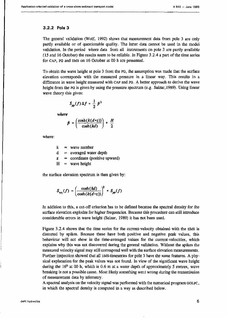
3.2.2 Pole 3
The general validation (Wolf, 1992) shows that measurement data from pole 3 are onlypartly available or of questionable quality. The latter data cannot be used in the modelvalidation. In the period where data from all instruments on pole 3 are partly available(15 and 16 October) the results seem to be reliable. In Figure 3.2.4 a part of the time seriesfor CAP, PG and EMS on 16 October at 00 h are presented.
To obtain the wave height at pole 3 from the PG, the assumption was made that the surfaceelevation corresponds with the measured pressure in a linear way. This results in adifference in wave height measured with CAP and PG. A better approach to derive the waveheight from the PG is given by using the pressure spectrum (e.g, Saizar,1989). Using linearwave theory this gives:
where
" { cosh(M) J 2
where:
k - wave number
d = averaged water depthz = coordinate (positive upward)H = wave height
the surface elevation spectrum is then given by:
In addition to this, a cut-off criterion has to be defined because the spectral density for thesurface elevation explodes for higher frequencies. Because this procedure can still introduceconsiderable errors in wave height (Saizar, 1989) it has not been used.
Figure 3.2.4 shows that the time series for the current-velocity obtained with the EMS isdistorted by spikes. Because these have both positive and negative peak values, thisbehaviour will not show in the time-averaged values for the current-velocities, whichexplains why this was not discovered during the general validation, Without the spikes themeasured velocity signal may still correspond well with the surface elevation measurements.Further inspection showed that all EMS-timeseries for pole 3 have the same features. A phy-sical explanation for the peak values was not found. In view of the significant wave heightduring the 16* at 00 h, which is 0.6 m at a water depth of approximately 5 metres, wavebreaking is not a possible cause. Most likely something went wrong during the transmissionof measurement data by telemetry.
A spectral analysis on the velocity signal was performed with the numerical program GOLPC,
in which the spectral density is computed in a way as described below.
delft hydraulics

Application-oriented validation of a cross-shore sediment transport modal H 840 — June 1993
The velocity time series is divided into a number of subseries, To avoid leaking of energydensity to neighbouring frequencies, a cosine tapering is applied. In the time domain thismeans that the discrete velocity signal is multiplied with a taper value given by:
where N = number of values of the velocity signal. Here the tapering was used in thefrequency domain. Applying the Harm taper then yields:
Z(k) = 4 2ft-1) + ~ *(*) - 74 2 4
j f c - 1 2 £ - 1
where 2{k) stands for the raw Fourier-transformed values of the velocity signal, Using ataper means that information at the beginning and end of the velocity time series is lost.This can be compensated by using half overlapping subseries. A spectral analysis of thesubseries is performed with DFT (Discrete Fourier Transformation):
JV~1 jZ(k) = £ z(n)e N
where:
2(k) complex and k = 0,1, ... N/2z(n) the values of data from subseries
which is solved with the FFT (Fast Fourier Transform).
The frequency interval is given by;
Finally, a smoothing was performed on the spectral values:
Z(k) = i Z(k-1) + I Z(k) + i- 2<Jc*l)4 2 4
* « 1,2, | -
yielding the energy density spectrum of the cross-shore velocity signal, presented in Figures3.2.5 and 3.2.6.
delft hydraulics

Application-oriented validation of a cross-shore sediment transport modal H 840 — June 1993
The following parameters have been presented in Figures 3.2.5 and 3.2.6:
• the zeroth order spectral moment mo = fo
• peak period Tp
• Nyquist frequency / L ? ~2Af
ci• frequency resolution BE = 2 —c2 Af+1
• degrees of freedom v = 2cvM
where M is the number of subseries used and c, and C2 coefficients depending on the taper-and smoothing functions. The spectrum derived from the cross-shore velocity signal showsthat it is difficult to use a low-pass Fourier filter to eliminate the spikes from the velocitysignal.
3.2.3 Frame
The frame was only operational during a relatively short period of time (15th to 19th ofOctober) covering the first part of the storm period. Figure 3.2.7 shows a part of thetimeseries obtained with the S4-sensor on 16 October at 00 h. Discontinuities in the signalare caused by the relatively low sampling frequency of 1 Hz. The minimum wave periodthat is still measured is determined by the Nyquist frequency:
1
This means no information is available on waves with periods shorter than 2 seconds. Thisis of less importance for the morphological validation, but for the hydraulic validation thehigher harmonics are also of importance; this with respect to the non-linearity of theincident waves.
Figure 3.2.7 shows that the wave height at the frame is significantly higher than measuredat pole 3. Because the wave height/water depth ratio is small for both locations, this cannotbe explained by shoaling effects only. In Figures 3.2.8, 3.2.9 and 3.2.10 statistical distribu-tions of the trough-crest values measured at 00 h 16-10-1991 using a Rayleigh distributionare presented. The distributions were obtained from the time series measured with the CAP-wire (Figure 3.2.8), PG at pole 3 (Figure 3.2,9) and S4 pressure sensor at the frame(Figure 3.2.10). Because the S4 used a lower sampling frequency, the time series obtainedby pole 3 were low-pass filtered before statistical analysis. It shows that the distributionsof the trough-crest values obtained at pole 3 with CAP and PG correspond reasonably well.To obtain the wave height at the frame and pole 3 with the pressure sensors, again theassumption was made that the surface elevation corresponds with the measured pressure ina linear way. This could explain the difference in wave height at pole 3 obtained with CAPand PG (Figures 3.2.8 and 3.2.9).
delft hydraulics

Application-oriented validation of a cross-shore sediment transport model H 840 — June 1993
It also shows that the wave height measured with the pressure sensors, that is exceeded fora given percentage, is considerably higher at the frame than at pole 3, The smaller waves(h/L0 > 0.5) will not be affected by shoaling and refraction while propagationg frompole 3 toward the frame. This means that the wave height measured with the pressuresensors, that is exceeded for 90% of the observations, should be of equal height for bothlocations. To achieve this the values for the pressure measured with the S4 pressure sensorat the frame should be multiplied with a correction factor. The factor derived from thetrough-crest distributions is given by:
= 0.63"90.fr
The same conclusion can be drawn from Figure 3.2.11 which shows the water levelmeasured at the frame, pole 3 and measured at Umuiden during 16 October. It shows thatthe water level measured at the frame is considerably higher than measured at pole 3 andUmuiden. The result of using the same correction factor as for the wave heights, is alsopresented in Figure 3.2.11. For the first part of the day it shows good correspondencebetween the water level measured at pole 3 and frame. Deviations in water level occur inthe second part of the day, with the beginning of the storm period. These deviations are dueto differences in wave set-up and surge level at the two locations.
3.2.4 Pole 2
The instruments on pole 2 were operational during a major part of the field campaign.Figure 3.2,12 shows a part of the time series obtained at pole 2 on 19 October at 15 h. Theupper graph shows the surface elevation measured with CAP and PG respectively. There isqualitative agreement between the two measuring devices, however the quanitative agree-ment is poor. The CAP measurements show sharp crested waves, whereas the PG showswaves of smaller wave height. A spectral analysis of the surface elevation signal obtainedwith the CAP presented in Figure 3.2.13, shows a peak in the wave energy for the firsthigher harmonic component (2*fp = 0.270 Hz). The sharp crestedness corresponds with thishigh non-linearity of the wave field. From Figure 3.2.11, which shows the water levelmeasured at pole 2 and Umuiden during 19 October, it follows that there is no apparentcalibration error in the CAP and PG measurements. Therefore it is likely that due to the highnon-linearity the method used to obtain the wave height from the PG measurements,hydrostatic approach, cannot be used here.
The measured velocity signals in both cross-shore and longshore direction are erratic,showing spikes similar to those observed at pole 3. The combination of approximately4 metres water depth with a significant wave height of 2 metres indicates that not muchwave breaking occurs at that moment. The spectra obtained from the velocity signals arepresented in Figures 3.2.14 and 3.2.15. These show that the spectrum derived from thecross-shore velocity signal does not correspond with the spectrum obtained from the surfaceelevation signal, whereas the spectrum derived from the longshore velocity signal does showmore qualitative agreement,
delft hydraulics

Application-oriented validation of a cross-shore sediment transport model H 840 — June 1993
Figure 3.2.12 also shows that the velocities in the longshore direction are high, which couldindicate that the angle of incidence is large at the time of measuring. However, this can alsoindicate that the orientation o f the EMS is different from the assumed orientation, Furtherinspection of the results obtained with the EMS in November show there is a strongcorrelation between the direction of the longshore current and that of the cross-shorecurrent. Figure 3.2.16 shows that if the longshore current flows in the northerly directionthe cross-shore current is directed in the offshore direction. If the long shore current isdirected toward the South the cross-shore current is directed onshore. A possible explanationfor this may be the way the current-velocity was measured, The instrument layout ispresented in Figure 3,2.17 which shows the radial cross-section of pole 2 and how the EMSwas attached to it, It also shows the stream lines of the flow field if potential theory is used.In the case of a positive longshore current the divergence of the flow field yields an offshoredirected component. A negative longshore current means that behind the pole the flow willconverge, yielding an onshore directed component. The fact that the offshore current-velocity is larger in general than the onshore directed current-velocity can be explained bythe offshore directed return flow and the vortex shedding which influences the flow fieldnear the EMS behind the pole in case of negative longshore current. The same phenomenaapplies for the measurements obtained with the EMS on pole 3.
Measurement data obtained with the EMS on pole 2 during October are in many cases onlypartly available or of questionable quality. According to the general validation the availabledata covers part of the storm and after storm period (18 - 23 October). The standarddeviations in current-velocity measured on the 18th are extremely high with peak current-velocities over 8 m/s. With a correspondng significant wave height of 2 metres this is mostunlikely. Therefore the EMS measurement data of 18 October has been excluded from themodel validation.
3.2.5 Pole 1
The instruments attached to pole 1 give information on water level and wave height only.These measurements have been available during most of the field campaign.
delft hydraulics

Application-oriBntad validation of a cross-shora sediment transport model H840 - June 1993
3.3 Morphological measurement data
3.3.1 Hydrographic surveys
The morphological evolution of the area of interest has been monitored by two hydrographicsurveys and several SAP-profile measurements. The echo soundings used in the hydrographicsurveys covered the area between beach pole 39000 and 40000 and the -2 to the -15 metresbottom contour line with a spacing between the survey lines of a 100 to 250 metres. Thedates on which the echo soundings were carried out, have been presented in Table 3.3.1.
description
hydrographic survey
hydrographic survey
date
13-09-1991
29-10-1991
Table 3.3.1 Dates hydrographic surveys
The bathymetry is presented in Figures 2.1.1 and 2.1.2 where the bottom level for pointsnot measured was obtained by interpolation performed with the DGM model. The fieldcampaign started on 09-10-1991, which is nearly a month after the first echo sounding. Inthis period there was a storm (H, = 3 m) so it is very likely that the bottom profile changedduring that period of time. To see which part of the bottom profile is morphologically stableon the time scale of the duration of the field campaign, two echo soundings along the 39500line were compared (see Figure 3.3.1). Due to small measurement errors this yields some-what erratic bottom profiles. This comparison shows that the differences in bottom depthfor the offshore part of the profile beginning at the top of the outer sand bar, are within themeasurement-error margin and therefore insignificant. The assumption that this part of thebottom profile is also representative for the beginning of the field measurement campaignis thus justified. However, it also shows some significant changes in the remaining part ofthe bottom profile between outer sand bar and beach. It is impossible to say whether thesechanges occurred during the field campaign or before that. The assumption that this part ofthe bottom profile is also representative for the beginning of the campaign is therefore notjustified.
delft Hydraulics 10

Application-oriented validation of a cross-shore sediment transport model H 840 - June 1993
3.3.2 SAP-profiles
The SAP was used to monitor the evolution of the beach and most shoreward sand bar. Thedates on which the SAP measurements were carried out have been presented in Table 3.3.2,
description
SAP
SAP
SAP
SAP
SAP
date
11-10-1991
14-10-1991
23-10-1991
30-10-1991
01-11-1991
Table 3.3.2 SAP measurements
The SAP measurements are presented in Figures 3.3.2 to 3.3.5. These show the bottomprofile of two successive measurements and their comparison in bottom depth that occuredin between the two measurements. The SAP covers the bottom profile from the beach to justpast the shoreward sand bar at beach pole 39500. Replacing the measurement data obtainedwith the echo soundings at beach pole 39500 with the SAP measurement of 11-10-1991increases the reliability of the bottom profile at beach pole 39500 for the beginning of themeasurement campaign. For the part of the bottom profile in between the two sand bars atthe beginning of the measurement campaign, no more reliable measurements than the firstecho sounding (13-09-1991) are available. It is assumed that this part is also representativefor the beginning of the field campaign, This is partly justified because there was a muchmore severe storm (Hs = 5 m) during the field campaign than in the period between thefirst echo sounding and the start of the campaign. It is therefore likely that most of thechanges in bottom configuration between the two sand bars occured during the fieldcampaign and not before.
delft hydraulics 11

Application-oriented validation of a cross-share sediment transport model H 840 — June 1993
4 Measurement data
4.1 Introduction
From the measurement data available, we selected representative periods for the modelvalidation. Using all the available measurement data would increase the amount of work tobe done considerably without yielding much additional information. The representativeperiods depend on the time scale of the processes to be validated. Because the hydrodynamicprocesses occur on a much smaller time scale than the morphodynamic processes, a shortervalidation period can be used in the first case than in the case of the morphodynamic modelvalidation. From the measurement-data validation (section 3.3) it follows that reliable dataon the bottom profile at beach pole 39500 are available from 11 October to 1 November.For the hydrodynamic validation, measurement data are available over a longer period oftime, from 8 October to 19 November. However, in this period not all instruments deployedhave been operational. Within these periods the representative periods for the modelvalidation have been selected.
4.2.1 Criteria for hydrodynamic validation
We defined the following criteria:
• accurate representation of the bottom profile• high spatial resolution
The local hydraulic conditions are dependent on the bathymetry, This means that an accuraterepresentation of the bottom profile is a necessity for the hydrodynamic model validation.The reliabilty of the measured bottom profile has its maximum on the day of measuring anddecreases with time as bottom changes occur. Because the bottom changes computed withthe model have to be validated also, the hydrodynamic validation should be performed witha constant bottom profile. This means that the hydraulic data set used in the modelvalidation should have been obtained in a period close to when the bottom profile wasmeasured. The length of the hydrodynamic validation period is thus determined by bothhydraulic and morphological conditions. Within this period significant changes in hydraulicconditions should occur in order to validate the model representation of the hydraulicparameters as a function of time. However, this period should still be small on themorphological time scale so no significant changes in the bottom profile have occured.
Morphodynamic behaviour (accretion, sedimentation) is determined by the local hydraulicconditions. This means that the hydrodynamic parameters should be validated as functionof time and space. The first is determined by the period of time in which measurement dataare available, whereas the latter is determined by the location of the various measuringpoints. The total number of measuring points along the 'coast-normal' is 5 (see section2,1). The wavec yields the incident wave field at the offshore boundary to be used as inputfor the model. This means that 4 measuring points along the 'coast-normal' were availableto perform the hydrodynamical model validation with. The measurement data obtained atpole 1 yields information on the surface elevation only.
delft hydraulics 12

Application-oriented validation of a cross-shore sediment transport model H 840 - June 1993
4.2.2 Selection of data for hydrodynamic validation
If the velocity measurement data obtained with the EMS at pole 3 are excluded from themodel validation, the availability and reliability of the measurement data show that it is notpossible to comply with both criteria mentioned in Section 4.2.1. In that case the maximumspatial resolution for the velocity-related parameters is restricted to two measuring points,frame and pole 2 on 19 October. On other days only one of these measuring points wasavailable. Figure 3.3.3 shows that between the 14th and the 23rd significant changes occuredin the bottom profile at beach pole 39500. The fact that the 19"1 is in the middle of thestorm period means that no accurate information on the bottom profile for this day isavailable. The use of this data set does therefore not comply with the first criterion.
Including the velocity measurements obtained at pole 3, assuming that the the reliability ofthese can be increased, yields the measurements obtained on the 16th of October as apossible data set. During this day all instruments except the EMS to measure the longshorevelocity at pole 2 were operational during a period of approximately 18 hours. Within thisperiod the hydraulic conditions develop from being quiet to stormy, thus showing asignificant change in hydraulic conditions. The last SAP-profile measurement before the 16th
was performed on the 14th of October. In the period between these two dates the hydraulicconditions are very mild. The comparison of SAP-profile measurments taken on the 11th andthe 14th of October presented in Figure 3.3.2, show negligible differences in bottom level.Because the hydraulic conditions on the 15th of October are similar to the ones in this periodno significant bottom changes are expected to occur on this day either. This means that thebottom profile on the 16th of October can be represented accurately.
Both data sets have been used in the hydrodynamic model validation. The reason for thisis the limited reliability of both the velocity measurement data obtained on the 16th at pole3 and the bottom profile at beach pole 39500 on 19 October. The latter is a combination ofthe echo sounding on 29-10 and the SAP-profile of 23-10. This combination is based on theassumption that most of the morphological changes occured during the first part of the stormwhen the profile is most out of storm-equilibrium. Deviations between actual and assumedbottom profile on the 19111 are most likely to occur in the part between the beach and theouter sand bar. This is due to the recovery of the bottom profile in the after storm periodfrom 19 to 23 October. This recovery is already included in the echo sounding and SAP-profile. The recovery is confirmed in Figure 3.3.5 which shows the profile developmentof the inner sand bar between 30 October and 1 November. The top of the sand bar ispropagating in the onshore direction.
With the selected data sets two hydrodynamical computations were carried out as presentedin Table 4.2.1.
run id
hi
h2
period
16-10
19-10
profile
echo 13-09
SAP 14-10
echo 29-10
SAP 23-10
Table 4.2.1 Run identification hydrodynamic computations
delft hydraulics 13

Application-oriented validation of a cross-shore sediment transport model H 840 — June 1993
4.3,1 Criteria for morphodynamic validation
definition of criteria
• hydraulic boundary conditions
• measurement data covers the active profile• high resolution in time
As mentioned before (Section 4.2.1), the local sediment transport depends on the hydraulicboundary conditions. To compute the profile development these hydraulic boundary condi-tions have to be used as model input. This means that information on the incident wavefield, water level and tidal velocity has to be available for the period for which the morpho-dynamic model representation is validated.
The active profile is defined as that part of the bottom profile in which morphologicalchanges occur on the time scale of storm events, If all of this bottom profile is included inthe measurements, it is possible to estimate the net sediment balance between two measure-ments. This is done by computing the total volume of sand above a reference level. Thislevel should be at a depth beneath which the changes in bottom level are insignificant. Thenet sediment balance can then give an indication whether the bottom changes observedbetween two measurements are due to two-or three-dimensional effects. This is essential forthe interpretation of the differences occuring between the measured bottom level and thecomputed bottom level. If the net sediment balance is non-zero this means that sediment hasbeen transported in the longshore direction. However, if the net sediment balance equalszero, this does not necessarily mean that sediment has been redistributed along the profile.It can still have resulted from longshore sediment transport. In fact, it is not possible toderive the magnitude and direction of the sediment transport rates from seabed topographysurveys only (de Vriend et al, 1987) unless the transport direction is known. This is shownin Figure 4.3.1.
The second criterion depends on the morphological time scale, which is merely determinedby the storm events in which large amounts of sediment are redistributed along the profile.This results in significant changes of the bottom profile, which should be monitoredfrequently for the model validation. This will show the development of the bottom profileduring the various sea states.
If the measurements comply with both criteria and it is assumed there is no longshoiesediment transport gradient (uniform in longshore direction) it is possible to estimate thetime-averaged sediment transport rates which occured between two measurements. Thedifference in transport between two points can be computed with:
Including the active profile in the bottom profile measurements gives a point with zerotransport at the offshore boundary, which means that the sediment transport in the otherpoints can be computed. If the period in between two bottom profile measurements isrelatively small, this method yields information on the sediment transport during differentsea states which can be used in the model validation.
delft hydraulics 1 4

Application-oriented validation of a cross-shore sediment transport model H 840 - June 1993
4.3.2 Selection of data for morphodynamic validation
Because the hydraulic measurements cover a longer period of time than the morphologicalmeasurements, the first criterion can be complied with.
As shown in Section 3.3 there is only a limited number of profile measurements available.None of these single measurements include the active profile. What can be achieved bycombining the echo soundings and SAP-profile measurements (see Table 4.1). It is then alsopossible to estimate the time-averaged sediment transport rates along the profile. However,with the available instruments it was not possible to perform any bottom profile measure-ments during storm conditions. Therefore, all profile measurements had to be carried outduring quiet sea states, which means that the time interval between two measurements canbe large. This makes it impossible to relate the computed time-averaged sediment transportsto a certain sea state and is thus of less interest for the model validation.
For the morphodynamic validation the echo soundings and SAP profiles have been combinedas presented in Table 4.3.1.
period
beginning field campaign
before storm period
after storm period
profile
echo 13-09-1991 + SAP 11-10-1991
echo 13-09-1991 + SAP 14-10-1991
echo 29-10-1991 + SAP 23-10-1991
echo 29-10-1991 + SAP 30-10-1991
Table 4.3.1 Combined bottom profiles
Here the assumption has been made that all significant changes in the part of the bottomprofile which was not covered by the SAP occurred during the storm period from 16 to21 October. This means that in the period before the storm this part of the bottom profileis represented by the first echo sounding (13-09-1991) and after the storm by the second(29-10-1991). Figures 3.3.2 to 3.3.5, which present the SAP profiles, indicate that thisassumption is justified. These Figures show that no significant changes in the bottom profileat the offshore end of the inner sand bar occurred except during the storm period. Withthese data three morphodynamic computations were performed as presented in Table 4.3.2.
run Id
ml
m2
m3
period
11-10 to
14-10 to
23-10 to
14-10
23-10
31-10
calm
storm
calm
remarks
sea state
+ after storm
sea state
conditions
Table 4.3.2 Run identification morphodynamic computations
delft hydraulics 15

Application-oriented validation of 8 cross-shore SBdiment transport model H 840 — June 1993
5 Model description
5.1 Introduction
With the data sets selected the application-oriented model validation can be performed. Toshow in what way the various hydraulic and morphological processes have been modelled,a brief description of the model UNIBESTTC is given in the next two sections, UNIBEST TC
is a numerical model used to predict the profile changes of uniform beaches due to wave-induced cross-shore sediment transport. The model consists of different modules shown bythe flow diagram in Figure 5.1.1, Given the hydraulic input conditions, such as incidentwave field, water level and tidal current the local instantaneous velocity due to waves,longshore current and return flow is computed by the hydrodynamic modules. Given thetime-averaged local flow velocity, the sediment transport rates and corresponding profilechanges are computed. The symbols used in the model description in Sections 5,2 and 5,3are defined in the list of symbols.
5.2 Hydrodynamics
The wave propagation of the incident wave field is computed with the wave energy decaymodel of Battjes and Janssen (1978). It includes the wave energy changes due to bottom-and current refraction, shoaling, bottom dissipation and wave breaking. The boundarycondition is given by the wave energy, wave frequency and wave direction measured at thewavec.
Adx
cg cos6w Ag cos6w + * + -J.
where:
E = wave energyDb ~ wave energy dissipation due to wave breakingDf = wave energy dissipation due to bottom friction
The wave energy dissipation due to bottom friction Df is given by:
*-iwhere Cf represents the bottom friction factor.
delft hydraulics 16

Appticatlon-orlented validation of a cross-shoro sadiment transport model H 840 — June 1993
Using a Rayleigh distribution for the non-breaking waves to relate the probability of wavebreaking to a given wave field with H ^ wave height, the fraction of breaking waves iscomputed:
and
Hm = (0.88/fc) tanh (vAft/0.88)
where 7 is the wave breaking parameter.
The dissipation of wave energy in a random wave field for breaking waves is modelled witha bore:
The dissipation of wave energy due to wave breaking yields a driving force for bothlongshore current and return flow. The longshore velocity is obtained from the longshoremomentum equation. This equation describes the balance between the driving forces of thelongshore current due to the tide and waves and the bottom friction for combined waves andcurrent:
where:
iy = surface slope in longshore directionfcw = bottom friction for combined current and wavesV = longshore current velocity
The first term on the left is due to the tidal current. Given the tidal current at a referencedepth as input, the corresponding surface slope is computed from the longshore momentumbalance without waves.
The combined friction factor is given by:
fm = exp[-5.977 + 5.213 (abfr ) " m ] * 181og(12A/i*fe)
where:
ab = the amplitude of the horizontal orbital excursion near the bottomr = two and a half times the median grain size Dso
rkls = bottom roughness
delft hydrauiios 1 7
Application-oriented validation of a cross-shore sediment transport model H 840 — Juris 1993
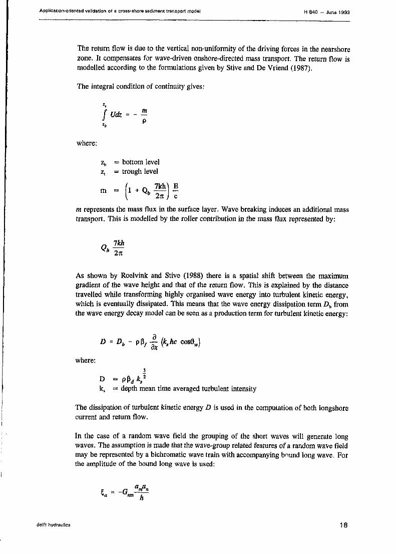
The return flow is due to the vertical non-uniformity of the driving forces in the nearshorezone. It compensates for wave-driven onshore-directed mass transport. The return flow ismodelled according to the formulations given by Stive and De Vriend (1987).
The integral condition of continuity gives:
f Cftfc * - £i P
where:
4 = bottom levelzt = trough level
m represents the mass flux in the surface layer. Wave breaking induces an additional masstransport. This is modelled by the roller contribution in the mass flux represented by:
Ikh
As shown by Roelvink and Stive (1988) there is a spatial shift between the maximumgradient of the wave height and that of the return flow. This is explained by the distancetravelled while transforming highly organised wave energy into turbulent kinetic energy,which is eventually dissipated. This means that the wave energy dissipation term Db fromthe wave energy decay model can be seen as a production term for turbulent kinetic energy:
D=Db-
where:
k, ~ depth mean time averaged turbulent intensity
The dissipation of turbulent kinetic energy D is used in the computation of both longshorecurrent and return flow.
In the case of a random wave field the grouping of the short waves will generate longwaves. The assumption is made that the wave-group related features of a random wave fieldmay be represented by a bichromatic wave train with accompanying bound long wave. Forthe amplitude of the bound long wave is used:
delft hydraulics 1 8

Application-oriented validation of a cross-shore sediment transport model H 840 - June 1993
In which short wave amplitudes are given by:
1 2 1 2 _ 1 ff 2
where the condition that the schematized wave train has the same surface variance as therandom wave has been used. The individual velocities are obtained using linear wavetheory,
For the long wave component calculated as:
The near bottom time-varying flow due to short and long waves is given by:
with the beat frequency Aw = &>p
The orbital velocities near the bed due to short waves, which determine the strength of theonshore directed wave asymmetry transport, have been computed using the model RFWAVE,
developed at DELFT HYDRAULICS (G. Klopman, 1989). It is based on the Fourier approxima-tion of the stream function method as developed by Rienecker and Fenton (1981), usingwave energy as input.
delft hvdraulics ' °

Application-oriented validation of a cross-shora sediment transport model H84O - June 1993
5.3 Morphodynamics
The sediment transport is calculated according to the formulations given by Baiiard (1981),of which only the cross-shore component is used for the time-dependent morphologicalcomputations. This formulation includes transport due to the combined actions of steadycurrent, wave orbital motion and bottom slope effect.
The Baiiard transport model in two horizontal dimensions is given by:
AgN tan<|>
AgN w w
Hy AgN tan* < | a |2 a > - = % < | ay tan<J)
AgN wa |3 a > - -! tanpy < I a |5 >
w
where:
cf = 0.5 fwfw = exp [-5.977 + 5.213 (ab/r)-
194]< > = indicate averaging over time.
The longshore transport is defined as the component of the total transport vector inlongshore direction,
The bottom level changes are computed from the mass balance:
dz•at
delft hydraulics 20

Application-oriented validation of a cross-shore sediment transport model H 840 — June 1993
6 Processing measurement data
6.1 Introduction
The data sets to be used in the model validation still have to be processed for two purposes.Firstly, to generate input data for the UNIBESTJTC computations and secondly, to make adirect comparison between model output and measurement data possible. To do so thevelocity measurement data obtained at pole 3 and pole 2 have to be corrected first.
6.2 Correction of velocity measurements data
As shown in Figure 3.2.4 the instantaneous velocity signal obtained with the EMS at pole3 contains so-called spikes, which render the data useless for the model validation. In orderto extend the number of measuring points along the profile, this signal had to be corrected.
As mentioned earlier (see Section 3.2.2), the use of a Fourier filter technique to eliminatethe spikes from the velocity signal at pole 3 is not possible. A correction of the velocitysignal in the time domain was used instead. First the spike is detected, then replaced witha value obtained with a linear fit. The spike detection is based on the determination of thelocal maxima and minima in the velocity signal. Given a local maximum (or minimum) thecorresponding flow acceleration is determined. If this acceleration is much larger than tobe expected from linear wave theory, the value is replaced. This results in the velocity sigalas presented in Figure 6.2.1 It shows that in places were spikes have been replaced, thevelocity signal is somewhat erratic. Low-pass filtering (fpass = 1 Hz) of this velocity signalresults in the time series as presented in Figure 6.2.2. It shows good correspondance withthe surface elevation for both the cross- and longshore velocity. Spectral analysis of thesurface elevation and the corrected velocity signal results in the energy density spectrapresented in Figures 6.2.3. to 6.2.5. The correspondence between the energy density spectraderived from the surface elvation and velocity measurements is good, except that there issome spurious high frequency energy in the velocity signal,
At pole 2 a similar procedure was followed to obtain the corrected velocity signal. Theresult for the time series at 15 h is presented in Figure 6,2.6. and the spectrum derived fromthe cross and longshore velocity signal in Figures 6.2.7 and 6.2.8.
After the first correction of the velocity signals obtained at pole 3, the time-averaged valuesof the cross- and longshore velocities were computed, These are presented in Figure 6,2,9along with the time-averaged velocities at the frame. The current-rose for both pole 3 andframe is presented in Figure 6.2.10. These figures show there is an offset for the cross-shore directed cur rent-velocities measured at pole 3. The offset value was determined byselecting a time point with a calm sea state and zero longshore current. From Figure 6.2.9it then follows:
T = 5.4 hoffset = -0,1 m/s
dBlft hydraulics 21

Application-oriented validation of a cross-shore sediment transport model H 340 — June 1993
The calm sea state means that there are no breaking waves near pole 3 (water depth ofapproximately 5 m) so the return flow should be negligible, which is in correspondance withthe time-averaged cross-shore velocity measured at the frame for T = 5.4 h, The cross-shore directed velocity signal becomes:
uc - u + 0.1 m/s
The current-rose for pole 3 (see Figure 6.2,10) shows a similar deviation of the currentvelocities as was measured at pole 2 (see Figure 3,2.16). A possible explanation for this waspresented in Section 3.2.3. Assuming a virtual rotation of the EMS instruments of-8 degreesw.r.t. North, the correction for the velocity signals at both locations is then given by:
• 8 )
v2)*cos(ot + 8)
where a stands for the wave angle w.r.t. North (positive clockwise),
6.3 Input data UNIBEST TC computations
Generating the input files means that
• incident wave conditions• water level• tidal velocity• bottom profile• medium grainsize D50
• sediment fall velocity w
have to be obtained from the measurements.
In addition the following parameters have to be defined:
• wave breaking parameter 7
• bottom roughness rkls• bottom friction factor waves /w
• grid size dx
For the hydrodynamic model validation two data sets and for the morphodynamic modelvalidation three data sets were used (see Section 4). This means that 5 UNlBESTTC-inputfiles had to be generated.
delft hydraulics 2 2

Application-oriented validation of a cross-shora sediment transport model H 840 — June 1993
6.3.1 Incident wave field
The WAVEC yields the incident wave field at the offshore boundary giving:
• significant wave height Hs
• peak period Tp
• wave direction <x
The model uses the root mean square wave height, H ^ , as input. This means that the Hs
has to be translated to the H ^ . We assumed that the wave heights at the WAVEC areRayleigh distributed:
Pr
where
.(Jt\> H) = e \Sm0>
and E stands for the wave energy.
Based on this distribution the following relationship can be derived:
!!„-0.706H,
Where Hs is the significant wave height obtained from the measurements. However thereis a small difference between the measured and predicted significant wave heights (Goda,1974) which results in the following empirical relationship:
Hms = 0.744 Hs
which was used throughout the validation proces.
The wave direction for the incident waves at the offshore boundary has to be given w.r.t,the coast normal at Egmond aan Zee, where the wave directions obtained with the WAVEC
are w.r.t. North. Therefore the wave direction has been rotated in the following way:
acn = «wavec + 82°
The peak wave period measured at the WAVEC can be used directly as input for the model.
The incident H ^ , wave direction (positive counter clockwise) and peak period used in thecomputations have been presented in Figures 6.3.1 to 6.3.5.
delft hydraulics 2 3

Application-oriented validation of a cross-shore sediment transport model H 840 — June 1993
6.3.2 Water level
The WAVEC gives no information on the mean water level, but the instruments at the frameand poles do. There is additional information on the water level given by measurements atIJmuiden, located approximately 17 km to the South of Egmond aan Zee, The mean waterlevel is a combination of mean sea level, tidal elevation, surge level and wave set-up. Ofthese only the wave set-up is computed in the model. The other constituents have to beintroduced as boundary conditions. In Figure 3,2.11 the mean water level measured on16 October at the frame, pole 3 and IJmuiden have been presented, Due to the limited waterdepth at pole and frame these measurements include wave set-up. This is not so for themeasurements at IJmuiden. This is shown in Figure 3.2,11 where during the first part ofthe day, with a calm sea state, the agreement between the measured mean water levels atthe various locations is good. As the storm begins, the differences in measured mean waterlevel increases. This is due to the increased wave set-up in the surfzone. It also shows thatthe wave set-up at the frame during the storm is higher than at pole 3, which correspondswith the water depth at both locations. Based on these results the mean water level measure-ments obtained at IJmuiden were used as input for the model. The mean water-level inputfor the different model computations is presented in Figures 6.3,6 and 6.3.7.
6.3.3 Tidal current
The velocity measurements at frame and pole 2 and 3 have been used to obtain the tidalcurrent. The time-averaged velocity is a combination of tidal current, return flow, wave-induced longshore current and net velocity due to non-linearity of the waves. The time-averaged velocities measured at pole 3 and frame on 16 October are presented in Figure6.2.9. It shows that during this day there is a significant increase in both cross- andlongshore cur rent-velocities as the storm developes. The wave breaking induces anadditional longshore current and return flow. In absence of wave breaking at these locationsduring the first part of the day, the tidal current is directed alongshore. The tidal variationin the cross-shore direction is negligible. The tidal current can thus be obtained from thelongshore velocity measurements only. A filtering technique on the time-averaged velocitieswas used to obtain the M2 and M4 components of the tidal current. This was done bycomputing the Fourier transform of the time-averaged velocity signal. An inverse Fouriertransform of the high- and low-passed signal then results in the current velocity as presentedin the lower graph of Figure 6.3.6. The same procedure was followed to obtain the tidalcurrent-velocities for the other UNIBESTTC computations. The total time-averaged velocitieswere obtained from either pole 2, pole 3 or the frame depending on the availability. Theresulting tidal current-velocities for the various runs have been presented in Figures 6.3.6and 6,3.7.
delft hydraulics 2 4

Application-oriented validation of a cross-shore sediment transport model H 840 - June 1993
6.3.4 Bottom profiles
The bottom profiles obtained with the echo sounding show an erratic behaviour (see Figure3.3.1), To improve this, a weighted moving average technique was used to smooth thebottom profiles. After that the echo sounding and SAP-profile were combined to yield thedesired bottom profiles. The resulting profiles for the model computations have beenpresented in Figures 6.3.8 and 6.3.9.
6.3.5 Parameter settings
During the measurement campaign bottom samples were taken at Egmond aan Zee. Theresults at beach pole 39500 have been summarised in Table 6.3.1 derived from the DataSummary Morphological Measurements (Wolf, 1992).
location
dune foot
water line
1" trough
inner sand bar
2nd trough
outer sand bar
D 5 0 (/tin)
248
350
290
263
470
208
Dao <>m)
310
555
480
470
750
260
w50 (mm/s)
29.5
46.0
36.5
32.5
63.0
22.5
Table 6.3.1 Bottom samples near beach pole 39500
There is a large variation in the D50 along the bottom profile. The model uses a single valuefor the median grain size along the profile. In the model computations the following valueswere used for median grain size and fall velocity:
D50 = 280 urnw = 3 5 mm/s
The bottom roughness rkls is used to compute the friction factor for steady currents (waveinduced longshore current and return flow). The value used in the model computations isset to:
rkls = 500
which is of the order of DM.
The friction factor used in calculating the wave energy dissipation due to bottom friction is
set at:
fw = 0.01
where the value of fw is based on previous tests and measurements,
delft hydraulics 25

Application-oriented validation of a cross-shore sediment transport model H 840 - June 1993
The wave propagation module in UNIBESTTC uses a single value for the wave breakingparameter 7. In a model computation the incident wave height and wave period at theoffshore boundary will change, requiring different values for 7 (Battjes and Stive, 1985).A single representative value for the wave breaking parameter has to be defined. The valuefor the wave breaking parameter as function of the steepness of incident wave field ispresented in Table 6.3.2.
0 . 0 0
0 . 0 1
0 , 0 2
0 , 0 3
0 , 0 4
7
0.5
0.63
0.73
0.61
0.85
Table 6,3.2 7 as ftinction of wave steepness
Based on the significant wave height and corresponding wave period of the incident wavefield in each model computation the values for 7 were determined from Table 6.3.2 bylinear interpolation.
The resulting wave breaking parameters to be used in each model computation are presentedin Table 6.3.3.
run id
h i
h2
ml
m2
m3
tm]
3 . 0
3.0
0.5
3 . 0
0 , 7
TP
U]
8
S
a
6
7
0.75
0.76
0 . 7 3
0 , 7 6
0 . 6 5
Table 6.3.3 y used in each model computation
6.3.6 Grid size
It is possible to define a non-equidistant grid for the model computations. In areas wherelarge gradients in wave energy are expected or complex bottom topography has to berepresented the grid size is chosen to be smaller. This means that at the sand bars and beachwhere strong wave dissipation may occur the grid size is small compared to furtheroffshore.
delft hydraulics 26

Application-oriented validation of a cross-shore sediment transport model H 840 — June 1993
6.4 Processing hydraulic measurement data
The measurement data for the two hydrodynamical computations is processed in such a waythat a direct comparison with the model output is possible. Prom the model description itfollows that the following hydraulic parameters are to be validated:
• root mean square wave height: Hms
• incident wave angle 0W
• wave induced longshore velocity: V,• return flow: Ur
• odd velocity moments: <MflMJB>
• even velocity moments: < Mr l n >
where:
u(t) represents the instantaneous velocity<ut\
n> denotes time-averaging
In addition the third-order velocity moment has been split up into different constituents by
defining:
U(t) = M + M
where:
u = the mean velocityu — the time-varying component
Using this in the expression for the third order odd moment (see appendix A) yields thefollowing constituents in the cross-shore direction:
• current-interaction gucx = «(«2 + v2)• wave-current interaction guwcx = <w(w2 + f>2) + 2MM2 + 2vvU>• wave interaction guwx = <ii(il2 + v2)>
and in the longshore direction
• current-interaction gucy = v(u2 + v2)• wave-current interaction guwcy = <v(u2 + *2) + 2vv2 + 2MVM>
• wave interaction guwy = <%U2 + v2)>
The wave interaction term is then split into short- and long wave contributions by defining:
where
MS = time varying short wave velocity«i = time varying long wave velocity
delft hydraulics 2 7

Application-oriented validation of a cross-shore sediment transport model H 840 — June 1993
Using this in the wave interaction term yields (see appendix A) for the cross-shore direction:
• short wave interaction gusx = <«a(«/ + v/)>
• short-long wave interaction guslx = <3«JMir2 + utvs
2 + 2«,v/*j>
and for the longshore direction:
• short wave interaction gusy = <v,(«/ + vs2)>
• short-long wave interaction gusly = <3v,v/ + vp* + 2wsvsv,>
This means that the different velocity components have to be derived from the velocitymeasurements. The procedure followed in this is presented in Figure 6.4.1. A spectral andstatistical analysis with GOLPC are performed on the surface elevation time series obtainedat the various locations. This yields the trough-crest distribution, significant wave height andsurface elevation energy spectrum. Using the empirical relationship between the Hs and theH ^ yields the latter. Using a Fourier filter on the velocity time series, where the low-passfrequency has been determined from the surface elevation energy spectrum, yields the highfrequency (short wave) and low frequency velocities. The low frequency velocity signal isthan demeaned to obtain the time averaged velocity and the instantaneous long wavevelocity. The velocity constituents are then used to compute the constituents of the velocitymoments.
The high frequency velocity signal is also used to compute the average angle of incidenceat the measuring locations. This yields information on wave refraction as the wavespropagate from the WAVEC toward the shore.
Given the high frequency cross-and longshore velocity, u and v as defined in Figure 6.4.2then:
yAw = »
m
Av = wm - v
where m - tana
The relative error is given by:
r = AH sina =^A«2 + Av2
which may be rewritten to:
AMAV = — (v - wm
delft hydraulics 2 8

Application-oriented validation of a cross-shore sediment transport model H 840 — June 1993
where:
2 r 2 = (2m2w2 + 2 (m2 - 1) Swv - 2wSvz)(1 + m2)2
Applying the least squares method yields:
(2m2az + 2(wi2 - l)2wv - 2m2v2) = 0(I + m ¥dm
with the solution for m given by
m = a ± \ja2 + 1
where a ~2SHV
Which defines the average wave direction.
delft hydraulics 2 9

Application-oriented validation of a cross-shore sediment transport model H 840 — June 1993
Validation model output
7.1 Introduction
In the hydrodynamic model validation, attention was focussed on the velocity-relatedparameters. The reason for this is that the wave propagation module as such has undergoneseveral validations already (Stive and Battjes,1985), In this case we expect the correspon-dence between measured and computed wave height to be less good, because of the constantvalue for the wave breaking parameter.
The constituents which make up the third-order velocity moment were validated as well.This because of the strong correlation between measured sediment transports and the third-order velocity moment (Al Salem and Ribberink,1992). The correlation coefficient (Cr)between the short-wave variance (short-wave energy) and the long waves to obtain the short-long wave interacton term, has not been validated separately. The correspondence betweenmeasured and computed values of Cr was proven to be poor in an earlier model validation(Saizar, 1990).
In the morphodynamic validation it was not possible to validate the sediment transport ratesalong the profile (see Section 4.3.2). However, based on the measured changes in thebottom profiles combined with the assumption of a uniform beach, a general direction,either on-or offshore, of the sediment transports can be estimated. The resulting profiles atthe end of each computation were compared with the measured bottom profiles.
7.2 Hydraulic validation
7.2.1 Wave height
Figures 7.2.1 and 7.2.2 show the measured and computed H ^ for both hydrodynamiccomputations, where the H^,, was derived from the pressure measurements with a linearapproach. The results for both CAP and PG correspond well during the 16th but not for the19th. The latter is most likely caused by a calibration error. Figure 7.2.1 shows that in runhi the lower wave heights during the beginning of the day are overestimated by the modelby both pressure sensors and capacitance wire, A possible explanation could be that thewavec overestimates the wave height ( H ^ = 0.5 m). However, as the storm develops ( H ^= 1.0 m) the correspondence between measured and computed wave height increases,which makes this explanation less likely. Assuming that the incident wave height at theoffshore boundary is correct, a lower wave height at pole 3 and frame results of thecombination of shoaling, refraction and directional spreading. The latter is not accountedfor in the wave propagation model. The directional spreading is most likely to be greaterduring relatively calm conditions than during the storm, which would explain why the waveheight is overestimated during the beginning of the day and not during the building of thestorm on the 16m. Later on the day the wave height at pole 3 is underestimated by themodel, indicating that the wave breaking parameter should have a higher value. Doing soimproves the results for the Hms at pole 3, but not so for the frame where in that case thewave height is underestimated even more. As for the second hydrodynamic computation(Figure 7.2.2) the measured and computed wave height show good correspondence for both
delft hydraulics 30

Application-oriented validation of a cross-shore sediment transport model H 840 - June 1993
pole 2 and frame (except for the PG as already mentioned), except at the end of the daywhere the wave height is overestimated. During this part of the day there is an increase inthe peak wave period but nearly constant value for Hms at the offshore boundary. This againindicates that the wave breaking parameter should be variable.
Both model computations show that the wave breaking parameter should be variable,depending on the incident wave conditions. This is even more important because thedissipation of wave energy induces cross- and longshore currents. Using a constant valuefor the wave breaking parameter can result in a time/spatial lag for these currents which isessential for the sediment transport.
7.2.2 Incident wave angle
Figures 7.2.3 and 7.2.4 show the measured and computed angle of incidence at the measur-ing points during the 16th and 19th respectively. In addition, it shows the angle of incidenceat the offshore boundary measured by the WAVEC. In general, the qualitative agreementbetween the computed and measured angle of incidence is good. However, there are somesignificant differences for the angle of incidence at the poles,
At pole 3 the quantitative agreement between the model output and measurements is notvery good. In general, it shows that the measured angle of incidence at pole 3 issignificantly larger than the model output. Due to bottom refraction the wave incidenceangle will decrease as the waves propagate toward the shore, but current-refraction due tothe presence of a longshore velocity gradient in the cross-shore direction, will have theopposite effect. In view of the approximately 1,5 m difference in water depth betweenpole 3 and frame and the small gradient in the longshore current, it is expected that theangle of incidence at both locations should be of similar order. This not being the caseindicates that the wave incidence angle at pole 3 is not correct.
There is a large difference between the wave incidence angle measured at pole 2 and frame.The water depth at pole 2 and frame are approximately the same, therefore this cannot becaused by bottom refraction, Current-refraction is not a plausible cause either as thelongshore velocity at the frame is higher than measured at pole 2. Therefore, the resultsobtained at pole 2 seem to indicate that the orientation of the EMS is different from the oneassumed (see section 3.2.3). This would mean that the orientation of the measuring devicehas changed during the measurement campaign, in view of the correlation diagram for thecurrent-velocities obtained in November (see Figure 3.2.16). This showed a rotation ofapproximately -8° with respect to the assumed orientation, These results indicate a rotationof approximately 30°, but in view of the limited number of measurements other causes arealso possible.
During the first part of 19 October the results for the wave incidence angle at the frameshow a difference of approximately 15°. At T = 0.5 d there is a shift in the measurementsresulting in very good agreement between the measured and computed wave incidenceangle. This shift is due to the heading of the frame, which has been taken into account inthe computation of the wave incidence angle. These results indicate that the heading of theframe did not change during 19 October, in contradiction with the measurements.
delft hydraulics 3 1

Application-oriented validation of a cross-shore sediment transport model H 840 — June 1993
7.2.3 Return flow
Figures 7.2.5 and 7.2.6 show the measured and computed return flow velocity. At thebeginning of the storm (Figure 7.2.5) this velocity is small, with an onshore directedcomponent near the bottom. Here the correspondence is good. As the incident wave heightincreases the return flow becomes offshore directed, increasing in magnitude for both pole3 and frame. This increase in return flow velocity occurs at a moment when the waveheight/water depth ratio at the frame is still small:
R = HJd = 0.4 atT= 0,375 days
which would indicate that wave breaking does not occur at these locations at that time.
Keeping in mind the water depth at both locations it is expected that there is a time lagbetween the return flow measured at pole 3 and frame. Also the magnitude of the velocityis expected to be smaller in the case of pole 3. In view of the various problems withmeasurement data obtained at pole 3, this could be caused by measurement errors. In bothcases the return flow is underestimated considerably, by the model with a maximum at T= 0.75 days corresponding with a low water level. Figure 7.2.6 shows a similar behaviourfor the return flow measured at the frame during the 19th. Except for the beginning of theday the return flow is significantly underestimated again. The measurements show anincrease in return flow as the water level decreases. The model results are just slightlyinfluenced by the changes in water level. As for pole 2 the measurements show an onshoredirected cross-shore flow during the first part of the measurements and an offshore directedflow during the last corresponding with increase in wave height. The model output showsa constant offshore-directed return flow.
7.2.4 Longshore velocity
In Figures 7.2.7 and 7.2.8 the computed and measured longshore velocities for 16 and19 October are presented. In the beginning of the storm (Figure 7.2.7) the tidal current isstill apparant, but as the storm increases this is overtaken by the wave-induced longshorecurrent. At the beginning of the storm the mean wave direction is from the South-West,inducing a positive longshore current. During the storm (Figure 7.2.8) the mean wavedirection is from the North-West generating a negative longshore current. The longshorecurrents at both pole 3 and frame increase in magnitude at T = 0.3 days, which is aroundthe same time that the return flow is increasing. The maximum longshore current- velocityduring the 16th (Figure 7.2.7) is measured at T = 0.75 days, coinciding with the maximumreturn flow velocity. Both Figure 7.2.7 and 7,2.8 show that the longshore current-velocityat the frame is overestimated considerably. At pole 3 there is initially an underestimation,but as the wave height increases the computed longshore current-velocity becomes of theright order. This is not so for pole 2 where the longshore current is underestimated at alltimes. These measurements indicate that in the case of a double bar system the longshorevelocity in the trough can be substantially higher than predicted. However, looking at thedevelopment of the longshore current at pole 2, caution is necessary. This because amaximium is expected at T = 0.75 days, corresponding with low water level and maximumwave height (see Figure 6.3.6),
delft hydraulics 3 2

Application-oriented validation of a cross-shore sediment transport model H 840 - June 1993
7.2.5 Even velocity moments
In Figures 7.2.9 to 7.2.14 the computed even velocity moments and those obtained fromthe measurements (see Section 6.4) are presented. These Figures show that the computedand measured data at the frame correspond quite well. The model output shows a moreerratic behaviour due to the higher output frequency (every 0.5 hours) compared to themeasured data (every three hours for the frame). This correspondence may seem somewhatsurprising in view of the significant differences between measured and computed longshoreand cross-shore cur rent-velocities. However, because the longshore current-velocity isoverestimated in the same order as that the return flow is underestimated, the total meanflow is still of the correct order at the frame. This is not so for pole 3, where the longshorecurrent is in the right order but the return flow is underestimated. This will result in anunderestimation of the even velocity moments. The rather large differences observedbetween measurements and computations at pole 3 cannot be explained by theunderestimation of the return current alone. Because:
<(«|2> = <w2 + 2«M + «2>
and by definition:
<2MM> = 0
which gives:
< | H | 2 > = M2 + <«2>
The total mean velocity is underestimted at pole 3 with approximately 10 %, which meansthat the difference between measured and computed orbital velocity is the cause for theobserved differences. The same goes for the results at pole 2 during the storm. Because thewave height and water depth at both frame and pole 2 are of similar order (H^ = 1.5 m,d = 3.5 m) and the total mean cur rent-velocity is smaller, the measured even velocitymoments are expected to be smaller in magnitude at pole 2. This not being the caseindicates that the measured orbital velocities at pole 2 ( and probably also at pole 3) maybe less reliable.
7.2.6 Odd velocity moments
Figures 7.2.15 and 7,2,16 show the cross-shore directed third-order odd velocity moment:
2 + v2)>
during the 16th and 19th respectively. These figures show that there are large differencesbetween the measurements and the model results. During most of the storm period themodel not only underestimates the magnitude of the velocity moment, but also the generaldirection of the velocity moment. In casu being onshore directed, whereas the measurementsshow an offshore directed velocity moment. The measurements at pole 2 show a rathererratic behaviour compared to the results at the frame.
delft hydraulics 3 3
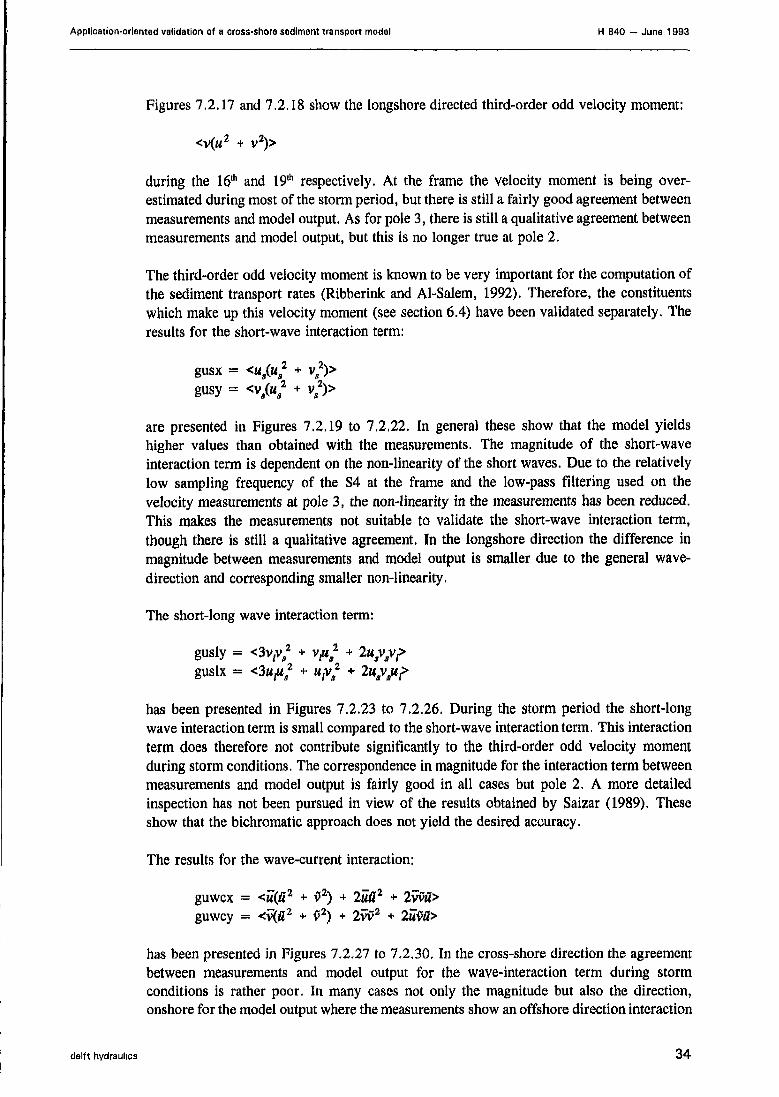
Application-oriented validation of a cross-shore sediment transport model H 840 — June 1993
Figures 7.2.17 and 7.2.18 show the longshore directed third-order odd velocity moment:
<V(M2 + v2)>
during the 16th and 19* respectively. At the frame the velocity moment is being over-estimated during most of the storm period, but there is still a fairly good agreement betweenmeasurements and model output. As for pole 3, there is still a qualitative agreement betweenmeasurements and model output, but this is no longer true at pole 2.
The third-order odd velocity moment is known to be very important for the computation ofthe sediment transport rates (Ribberink and Al-Salem, 1992). Therefore, the constituentswhich make up this velocity moment (see section 6.4) have been validated separately. Theresults for the short-wave interaction term:
gusx = <MS(«/ + vJ2)>
gusy = < v > / + v/)>
are presented in Figures 7.2.19 to 7.2,22. In general these show that the model yieldshigher values than obtained with the measurements. The magnitude of the short-waveinteraction term is dependent on the non-linearity of the short waves. Due to the relativelylow sampling frequency of the S4 at the frame and the low-pass filtering used on thevelocity measurements at pole 3, the non-linearity in the measurements has been reduced.This makes the measurements not suitable to validate the short-wave interaction term,though there is still a qualitative agreement. In the longshore direction the difference inmagnitude between measurements and model output is smaller due to the general wave-direction and corresponding smaller non-linearity.
The short-long wave interaction term:
gusly =guslx =
has been presented in Figures 7.2.23 to 7.2.26. During the storm period the short-longwave interaction term is small compared to the short-wave interaction term. This interactionterm does therefore not contribute significantly to the third-order odd velocity momentduring storm conditions, The correspondence in magnitude for the interaction term betweenmeasurements and model output is fairly good in all cases but pole 2, A more detailedinspection has not been pursued in view of the results obtained by Saizar (1989). Theseshow that the bichromatic approach does not yield the desired accuracy.
The results for the wave-current interaction:
guwcx = <ii(G2 + f*2) + 2««2 + 2vvfi>guwcy = <v(a2 + v2) + 2vv2
has been presented in Figures 7.2.27 to 7.2,30. In the cross-shore direction the agreementbetween measurements and model output for the wave-interaction term during stormconditions is rather poor. In many cases not only the magnitude but also the direction,onshore for the model output where the measurements show an offshore direction interaction
delft hydraulics 34

Application-oriented validation of a cross-shore sediment transport model H 840 - June 1993
term, is different. As for the wave-current interaction in the longshore direction, there isqualitative agreement between measurements and model output, except again for pole 2.Quantitatively it shows that at the frame the wave-current interaction term is overestimatedand is underestimated at pole 3 during storm conditions.
The current-interaction terms:
gucx = u(u2 + v2)gucy = v(«2 + v2)
have been presented in Figures 7.2.31 to 7.2.34. These show a similar results as for thewave-current interaction terms, except that the direction between measurements and modeloutput is the same.
The main contributions to the differences between the computed and measured third-orderodd velocity moment are due to the wave-current and current-interaction constituents. Theseconstituents are in general underestimated in magnitude in the cross-shore direction andoverestimated in the longshore direction. This is in correspondence with the observedoverestimation of the longshore current and underestimation of the return flow. Moststriking is the onshore directed wave-current interaction according to the model and theoffshore directed wave-current interaction in the case of measurements,
7.3 Morphodynamic validation
7.3.1 Profile development
The profile development for the three morphodynamic runs has been presented in Figures7,3.1 to 7.3,3. The first morphodynamic run: ml, shows little profile changes, except nearthe shoreline, This is not unexpected because the wave height is small (Hs < 0.5 m),meaning that wave breaking only occurs near the shoreline. Figures 7,3.2 and 7.3.3 showthe profile development during the storm and part of the after-storm period. During this runsome significant changes in bottom profile occur. During the first 3 to 4 days, when thewave climate develops from quiet to stormy, there is a flattening of both the inner and outersand bar. The trough between the inner sandbar and the shoreline is disappearing, As thestorm further develops only little changes occur in bottom profile at the inner sandbar,whereas the outer bar propagates in the onshore direction.
The comparison between measured and computed bottom profiles shows large differencesin bottom level. The development of the inner bar is completely different from the computeddevelopment. In reality the inner sand bar becomes more pronounced during this period. Italso shows a deepening of the trough between the shoreline and inner sand bar. The samegoes for the outer trough between the inner and outer sand bar which becomes deeper. Asmentioned before, it is difficult to say wether the deepening is a result of a gradient in thelongshore sediment transport rates or because of the redistribution of sediment along theprofile. The computations show little difference between the initial and computed bottomlevel in the second trough. The computed and measured development of the outer bar alsoshows large differences. The computations show a flattening of the outer bar and a propaga-
delft hydraulics 3 5
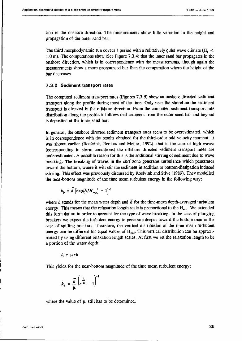
Application-oriented validation of a cross-shore sediment transport model H 840 — June 1993
tion in the onshore direction. The measurements show little variation in the height andpropagation of the outer sand bar.
The third morphodynamic run covers a period with a relitatively quiet wave climate (H9 <1.0 m). The computations show (See Figure 7.3.4) that the inner sand bar propagates in theonshore direction, which is in correspondence with the measurements, though again themeasurements show a more pronounced bar than the computation where the height of thebar decreases.
7.3.2 Sediment transport rates
The computed sediment transport rates (Figures 7.3.5) show an onshore directed sedimenttransport along the profile during most of the time, Only near the shoreline the sedimenttransport is directed in the offshore direction. From the computed sediment transport ratedistribution along the profile it follows that sediment from the outer sand bar and beyondis deposited at the inner sand bar.
In general, the onshore directed sediment transport rates seem to be overestimated, whichis in correspondence with the results obtained for the third-order odd velocity moment. Itwas shown earlier (Roelvink, Reniers and Meijer, 1992), that in the case of high waves(corresponding to storm conditions) the offshore directed sediment transport rates areunderestimated, A possible reason for this is the additional stirring of sediment due to wavebreaking. The breaking of waves in the surf zone generates turbulence which penetratestoward the bottom, where it will stir the sediment in addition to bottom-dissipation inducedstirring. This effect was previously discussed by Roelvink and Stive (1989). They modelledthe near-bottom magnitude of the time mean turbulent energy in the following way:
— 1-l
where h stands for the mean water depth and k for the time-mean depth-averaged turbulentenergy. This means that the relaxation length scale is proportional to the H^. We extendedthis formulation in order to account for the type of wave breaking. In the case of plungingbreakers we expect the turbulent energy to penetrate deeper toward the bottom than in thecase of spilling breakers. Therefore, the vertical distribution of the time mean turbulentenergy can be different for equal values of H ^ , This vertical distribution can be approxi-mated by using different relaxation length scales, At first we set the relaxation length to bea portion of the water depth:
I, = u*A
This yields for the near-bottom magnitude of the time mean turbulent energy:
* U )IT - —
where the value of \x still has to be determined.
delft hydraulics 3 6

Application-oriented validation of a cross-shore sediment transport model H 840 — June 1993
The additional stirring of sediment has been implemented in the Bailard sediment transportformulation in a similar way as described by Roelvink and Stive (1989). Using the resultsof the large-scale flume tests in the Grosse Wellenkanal (Roelvink, Reniers and Meijer,1992)to get an idea of the range of \JL results in:
0.2 < [x < 0.5
where \x = 0.2 corresponds to a calm wave climate with spilling breakers and \x =0.5corresponds to severe storm conditions with plunging breakers.
The result of an additional morphodynamic run: m2s with a stirring factor \x =0.35 hasbeen presented in Figures 7.3.6 and 7.3,7. This shows little improvement for the profiledevelopment at the inner sand bar. However, correspondence between the computed andmeasured profile development of the outer sand bar improves.
delft hydraulics 3 7

Application-oriented validation of a cross-shore sediment transport model H 840 — June 1993
8 Conclusions and recommendations
8.1 Field data
The measuring campaign carried out at Egmond aan Zee serves more goals then theapplication-oriented model validation of UNIBEST-TC. Therefore the general layout of themeasuring campaign has to comply with more criteria than those imposed by the modelvalidation. The recommendations presented here concern the model validation only.
From the measurement data validation it follows that as far as the velocity-relatedparameters are concerned, there is little spatial resolution. The number of velocitymeasuring points operative at the same time is two, during a relatively short period of time.This is mainly due to the malfunctioning of the EMS measuring devices. The data validationshows these instruments suffered frequent malfunctioning and breakdown. In cases wherevelocity signals obtained with the EMS are present, the model orientated validation showthese data have a low reliability. Where the time averaged current velocities may still becorrect, this is not so for the orbital velocities showing a rather erratic behaviour. Apossible cause for this behaviour seems to be the way the measuring is performed, with theEMS too close to the pole. Therefore the measurements are influenced by wave reflectionsand current deviations near the pole. The latter results in the strong correlation between thecross- and longshore current. It is therefore recommended to change the installation of theEMS at the poles, by increasing the distance between the measuring device and the pole.An important advantage of using the EMS to measure the velocities, is the possibility tocontinuously make long time series, which is important in the analysis of low-frequencyprocesses.
In view of the frequent malfunctioning of the EMS velocity meters, it is recommended tohave a possibility to check the time series and spectra while measuring. This couldconsiderably increase the operationally of the instruments.
The velocity measurements obtained with the S4 frame have proven to be very reliable, evenduring storm conditions. A disadvantage for the model validation was the low samplingfrequency of / Hz. This makes it impossible to measure the non-linearity of the wave field,responsible for the onshore drift velocity. The interval in between two bursts was threehours, due to which it was impossible to accurately follow the mean water level variations.Because the water level is of great importance to the hydrodynamic processes, it isrecommended to use shorter intervals. The combination of shorter intervals and highersampling frequency result in the necessity to extract the measurement data from the S4 datalogger much more frequently. Because during severe weather conditions the S4 can not beaccessed, this would result in monitoring only the first part of a storm. Installing a secondframe, which becomes operative after the first S4 is full, is a (expensive) possibility.
The wave height is monitored well as waves propagate from offshore toward the shoreline.The presence of five measuring points along the coast-normal results in a good spatialdistribution, where the locations of the measuring points are chosen well. The presence ofboth CAP and PG makes it possible to easily validate the surface elevation measurements.
delft hydraulics 3 8

Application-oriented validation of a cross-shore sediment transport model H 840 — June 1993
The morphological data proved to be insufficient to validate the model with. In order torelate various sea states to morphodynamic processes, measurements of the bathymetryshould be carried out much more frequently. The hydrographic surveys are importantbecause this shows whether profile changes in the cross-shore direction have resulted fromnon-uniformities in the longshore direction or not, It is known that the inner bar sometimesshows crescentic behaviour, which does not show in the bottom profile. If possible, it is alsorecommended to monitor the active profile, ranging from the outer bar to the beach, insteadof only just beyond the inner sand bar.
Summary
Conclusions:
• Measurement data obtained with EMS cannot be used to validate the model with.
• The morphological measurement data are insufficient to validate the model with.• Measurement data obtained with S4 are reliable and can be used for the model
validation.
Recommendations :
• Increased spatial resolution to monitor the velocity-related processes.• Different installation of the EMS current-velocity meters on the poles.• Possibility to check time-series and spectra while measuring.• Higher sampling frequency S4 to measure the non-linearity of the incident wave
field.• More frequent measuring of the bathymetry with SAP and hydrographic surveys.• Extend the SAP-measurements to include the active profile.
8.2 Model data
From the model-oriented validation of field data it follows that the velocity measurementsobtained at either pole during this field campaign have only limited value in the modelvalidation. Therefore, the conclusions and recommendations concerning the model aremainly derived from the frame measurements.
Some differences between measured a computed wave height were observed. How much ofthis difference is caused by the use of a constant value for the wave breaking parameter andwhich part is a result of the boundary condition given by the WAVEC-measurements, has stillto be determined. The same argument can be applied to the wave direction. The correspon-dence between the measured and computed angle of incidence at the frame seems to varywith the wave height. There is good correspondence for the higher waves but the angle ofincidence for smaller waves is less well predicted by the model. In general, the correspon-dence between the model output and the measurements for the wave height is good, butbecause better wave breaking formulations are present (Battjes and Stive, 1985, Roelvink,1991) it is recommended to improve the wave breaking formulation.
delft hydraulics 3 9

Application-oriented validation of a cross-shore sediment transport model H 840 — June 1993
The model considerably underestimates the magnitude of the return flow, which seems tobe in contradiction with earlier measurements (Roelvink and Stive, 1989) where reasonablecorrespondence was found. The main difference between the two sets of measurements isthe environment in which the measurement data were obtained. The measurements byRoelvink et al. were performed in a flume experiment whereas in this case field data isconcerned.
Several causes for the underestimation of the return flow can be thought of. Themeasurements could have been performed in a rip current, yielding a strong offshoredirected flow. Because no other current-velocity measurements outside the measurementarray are available, it is difficult to say whether this is the case or not, Another possiblecause could be the wind-driven return flow yielding an additional offshore directedcomponent at the frame. In view of the results obtained for the prediction of the longshorecurrent at the frame, which is significantly overestimated by the model, the wave-currentinteraction is also a possibility. This could possibly explain both the underestimation of thereturn flow and the overestimation of the longshore current, which cannot be explained bythe two mechanisms mentioned earlier.
There is a clear correspondence between the return flow and longshore current, where amaximum in magnitude of the longshore current corresponds to a maximum in the returnflow. Because the magnitude of the total time-averaged current-velocity is predicted withinthe right order, the wave-current interaction seems to result in a rotation of the total current,thereby increasing the return flow and decreasing the longshore current. Whether this is alsothe case for other points along the profile, has still to be determined.
The under- and over-prediction of the return flow and longshore current respectively, havea large influence on the magnitude and direction of the velocity moments. The predictionof the cross-shore directed third-order odd velocity moment shows poor correspondencewith the measurements. The major differences for this moment occur in the prediction ofthe wave-current and current constituents. It is recommended that the modelling of the wavecurrent interaction be improved.
An accurate prediction of the third-order odd velocity moment is extremely important withrespect to the sediment transport rates and directions. Due to the combined under- and over-prediction of the cross- and longshore current, the general direction of the cross-shore thirdorder odd velocity moment is onshore, yielding an onshore directed sediment transport. Thislatter is shown in the morphodynamic computations where the sediment transport is ingeneral onshore directed.
The model results for the development of the inner sand bar show little correspondence withthe measurements. However, the measurements can only be used as an indication and notfor a model validation. The introduction of additional stirring improves the results for theouter bar, but there are still significant differences.
delft hydraulics 40

Application-oriented validation of a cross-shore sediment transport model H 840 — June 1993
Summary
Conclusions:
• Important under-estimation of the return flow at the frame,• Longshore current at the frame is overestimated• Poor correspondence for the model prediction of the third-order cross-shore directed
velocity moment with the measurements.
Recommendations ;
• Incorporating improved wave-breaking formulation in the model.• Improve the model prediction for the longshore current and return flow. This will
also improve the prediction of the various velocity constituents.• Examine the wave-current interaction, being a likely cause for the over- and under-
estimation of longshore current and return flow respectively.
delft hydraulics

Application-oriented validation of a cross-shore sediment transport model H 840 — June 1993
References
Bailard, J.A., 1981. An energetics total load sediment transport model for a plane sloping beach. J. Geophys.Res., vol 86, no. C l l , pp. 10,938-10,954
Battjes, J.A. and J.P.F.M. Janssen, 1978. Energy loss and set-up due to breaking in random waves.Proceedings of the 16"1 International Conference on Coastal Engineering, pp. 569-587, AmericanSociety of Civil Engineers, New York,
de Vriend, H.J., R. Reinalda and H. Derks, 1987. The Egmond field data and their use for the validation ofmathematical models. Paper for SOOREAH-Seminar "Filed Measurements necessary for verification ofmorpholpogical numerical models", Grenoble, France,
Goda, Y., 1974. Proc. Int. Symp. on Ocean Wave Measurement and Analysis, New Orleans, Louisiana. NewYork, ASCE, vol 1, pp 320-337.
Groenendijk, F.C., 1992. TO-berekening, status quo van unibest-tc. RWS, Dienst Getijdewateren, rapportGWAO-92.194X.
Klopman, G., 1989. RFWAVE: Program for the computation of periodic gravity waves on a horizontal bottomusing the Fourier appriximation method of Rienecker and Fenton, DELFT HYDRAULICS, User manual.
Nairn, R.B., J.A.(Dano) Roelvink and H.N, Southgate, 1990. Transition zone width and implications formodelling surfzone hydrodynamics. Proceedings of the int. conf., vol 2, pp. 68-82, 22th CoastalEngineering Conference, Delft, The Netherlands
Ribberink, J.S. and A. Al-Salem, 1992. Sediment transports, sediment concentrations anJ bedforms in simulatedasymmetric wave conditions. Experimental study in the large oscillating water tunnel of DELFTHYDRAULICS, Data-report, H 840.20, part V.
Rienecker, M,M. and J.D. Fenton, 1981. A Fourier approximation method for steady water waves. J. FluidMech., vol 104, pp. 119-137.
Roelvink J.A. and M.J.F. Stive, 1989, Bar-generating cross-shore flow mechanisms on a beach. J. Geophys.Res., vol. 94, no. C4, pp. 4785-4800.
Roelvink, J.A., A.J.H.M. Reniers and Meijer, 1992. Large-scale flume tests in the Grosse Wellenkanal.Analysis of wave parameters and cross-shore transport and comparison with UNIBEST-TC. G6M,Coastal Morphodynamics, Final Workshop, abstracts-in-depth.
Saizar, A., 1990. The Egmond aan Zee field campaign, November-December 1989, and the use of the data forthe validation of a cross-shore sediment transport model. M.Sc. Thesis, Report H.H, 54, IHE Delft.
Sand, S.E., 1982. Long wave problems in laboratory models. J. Waterw. Port Coastal Ocean Div., Am. Soc.Civ. Eng., 108, pp. 492-503
Stive, M.J.F., 1986. A model for cross-shore sediment transport. Proceedings of the 20"1 InternationalConference on Coastal Engineering, pp. 1550-1564, American Society of Civil Engineers, New York.
Stive, M.J.F. and J.A. Battjes, 1984. A model for offshore sediment transport. Proceedings of the 19h
International Conference on Coastal Engineering, pp. 1420-1436, American Society of CivilEngineers, New York.
Stive, M.J.F. and H.J. de Vriend, 1987, Quasi-3D current modelling: wave induced secondary current. ASCESpecialty Conf. "Coastal Hydrodynamics", Delaware,
Stive, M.J.F and H.G. Wind, 1986, Cross-shore mean flow in the surfzone. Coastal Eng., 10,pp. 325-340.Wolf, F.C.J., 1992. Field measurements Egmond aan Zee, fall 1991. Data summary hydraulic measurements,
Parts I, II and III. Institute for Marine and Atmospheric Research, Department of Physical Geography,University of Utrecht.
Wolf, F.C.J., 1992. Field measurements Egmond aan Zee, fall 1991. Data summary morphological measure-ments. Institute for Marine and Atmospheric Research, Department of Physical Geography, Universityof Utrecht.
delft hydraulics Ref. •— 1
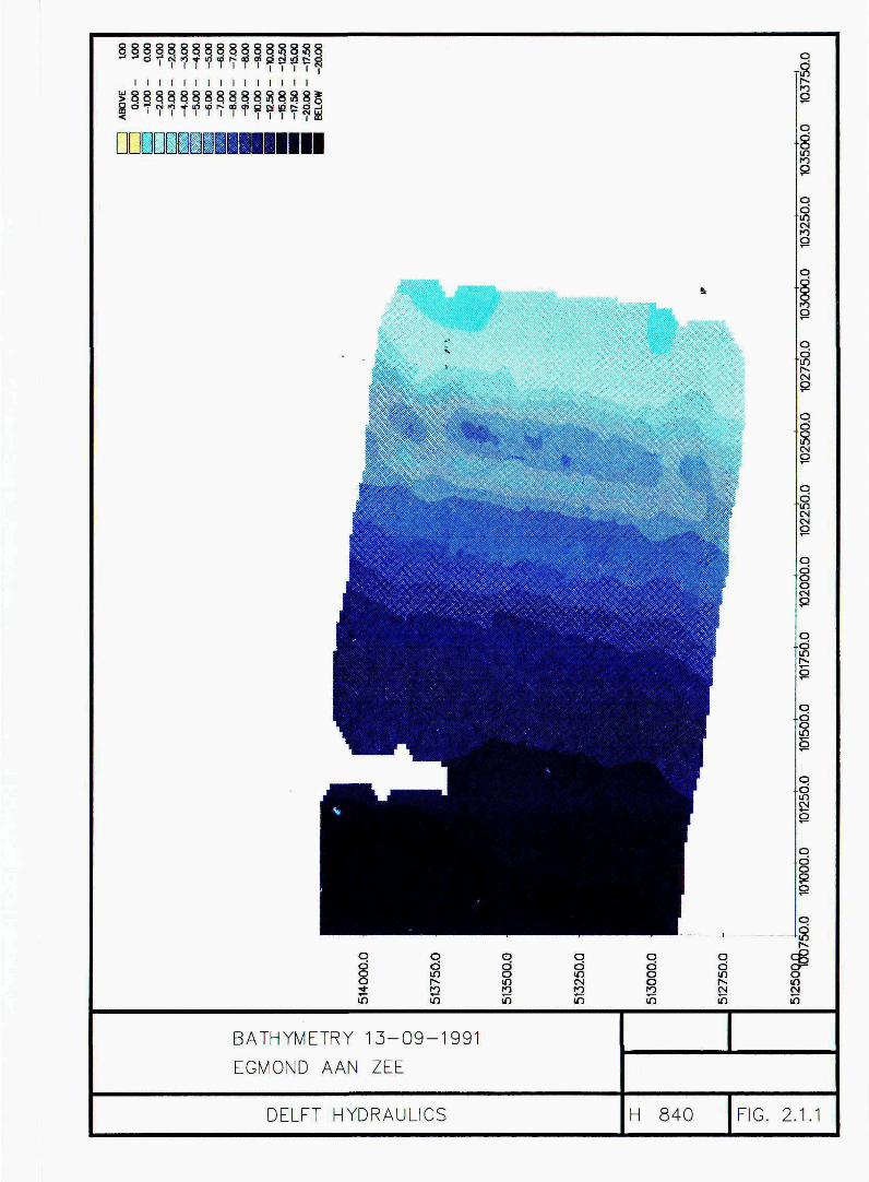
I I I I I I I I I I I I I I I
^3 ^J O ^3
I I I I•§Ss?§a
I I I I I
DDE
IT)
BATHYMETRY 13-09-1991
EGMOND AAN ZEE
DELFT HYDRAULICS H 840 FIG. 2.1.1
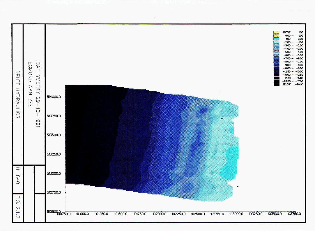
o73
a
o00
ooo
CD
ro
m CD
o >o 5:z: -<
mm
CD
o
co
514000.0
513750.0
513500.0
I - . ; - ; ' - • , : . , ,
513250.0
•
— —
^MWMBjPBB^BBH^ g
ABOVE0.00 -
-too --2.00 --3.00 --+.00 --S.00 --«.00 --7.00 --6.00 --9.00 -
-n.00 --1Z50 --6.00 --17.50 -
-20 .00 -BELOW
tootoo
0.00-too
-2JO0-AO0^ • - 0 0-5.00-6.00-7.00-8.00-9.00
-B.00-1250-15.00-1750-20.00
1Q1250.0 101500.0 101750.0 102000.0 102250.0 102500.0 102750.0 103000.0 103250.0 103500.0 103750.0

oa.
0)
Eo
ro
oa
o
GENERAL LAYOUT MEASURING POINTS
ALONG COAST NORMAL
DELFT HYDRAULICS H 840 FIG. 2.3.1

October 1991
m
o70
OCO
CO
O
P
rno
00
o2:Zio>
mXmo
6
5
4
A 3
(V
1
f \it Vrt
J \V
1*
10 15 20
time (days)
10 15 20
time (days)
25 30
November 1991
35
25 30 35

October 1991
om
o
o
<m
00
O
3]p
m
m
o
20
"
0
h ,__
rI .
TFT
20
I 1 5
3 10
0
10
10
15 20
time (days)
15 20time (days)
25
25
30
November 1991
30 35
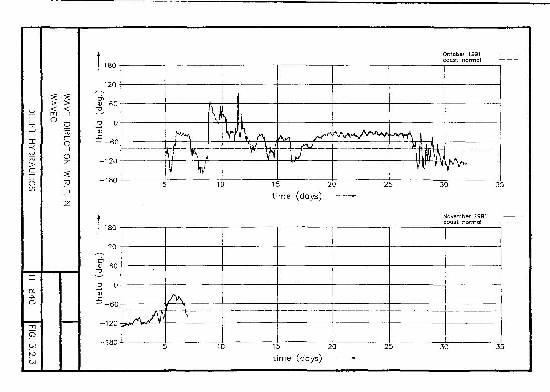
mr~~n—i
xo
o
00
o
p
ro
m mo gmoo
October 1991coast normal
-18010 15 20
time (days)25
I 180
120
Q> 6 0• — "
-120
-18010 15 20
time (days)25
30
November 1991coast normal
35
^ - \ —
30 35

CAPPG
100
-100
100
75
CO
Eo
-50
-75
-100 0
cross-shore velocity
SURFACE ELEVATION + ORBITAL VELOCITIES
POLE 3, 00 H, 16-10-1991
DELFT HYDRAULICS H 840 FIG. 3.2.4

8500
* " ^ 7500
vnnn
6500
I/I
A 6000 •CN•*
co 5500 •
EU
s • 5000 •
4500 •
y— 4000 •—
toUl 3500 •Q
O 3000 •
jJ
-U 2500 •
1S00 •
1000 •
500 -
0
11
J\
\
• " 1 —
Aw-—i
A
AA1
WA
—_-—,—-w
H - ^ — I •< 1.—•—.
•
•
•
I/'0.000 0,135 0.270 0.405 0.540 0.675 0.B10 0,945 1.080 1.215 1.350 1,485 1.620 1.755 1.890 2.025
FREQUENCY (HZ)
Mo =
4VM0 =
T p =
FNY =
DF =EDF =
1.05129.586,742.00000.0078
60Pole 3, EMS-x, 16-10-1991,
10 ^
00 h
(cm/s)*+2
cm/s
sHZ
HZ
ENERGY DENSITY SPECTRUM
DELFT HYDRAULICS H 840 I FIG. 3.2.5
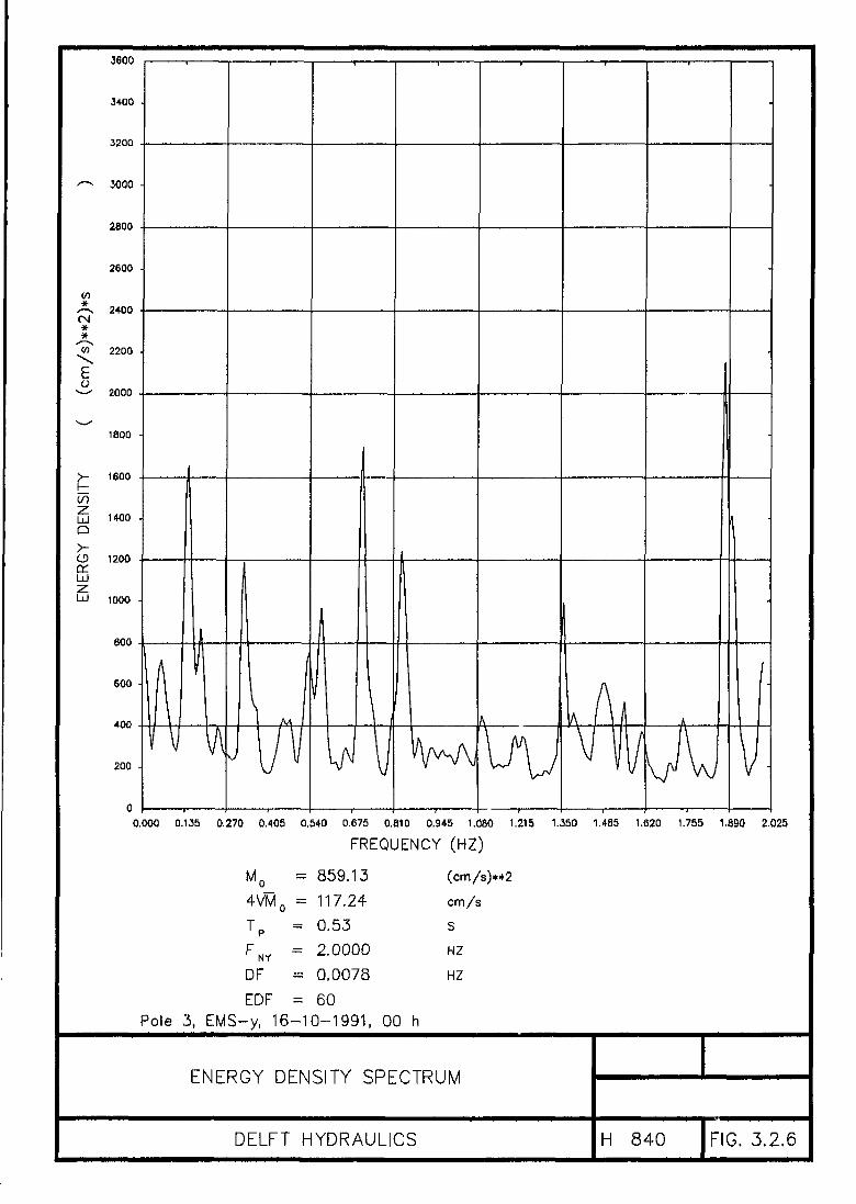
3600
3400 -
3200
0.000 0.135 0.270 0.405 0.540 0.675 0.810 0.945 1.080 1.215 1.350 1.4S5 1.620 1.755 1.890 2.025
Mo =
4VM0 =
T p =
F NY =
DF =
FREQUENCY
859.13
117.24
0.53
2.0000
0,0078
(HZ)
(cm/s)*+2
cm/s
S
HZ
HZ
EDF = 60Pole 3, EMS-y, 16-10-1991, 00 h
ENERGY DENSITY SPECTRUM
DELFT HYDRAULICS H 840 FIG. 3.2,6
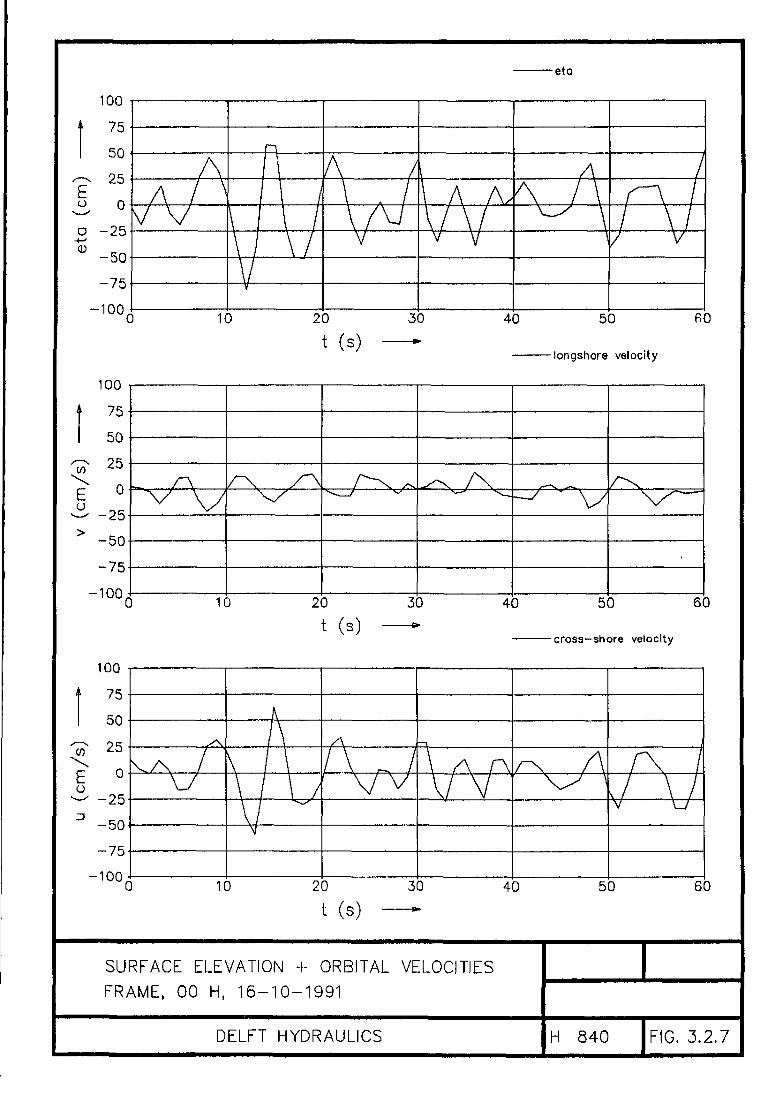
-eta
Eo
100
75
50
25
o -25
^ -50
-75
-100
100
75
50
AA 1 \
V V
n
1\ \ 1\ /vV
A i\ . / \ A A,
v V
A^ / \
ir\ // \/ v
10
25
E 0 =-
-25
-50
-75
-100
100
75
50
25
10
o-25
1 -50
-75
-10010
20t (s)
30
20
t (s)30
20
t (s)30
40 50 R0
-longshore velocity
40 50 60
-cross—shore velocity
A
v/\ /V/
A,A\V "
/ V „ /V v\ A r\Vv
A-N /Ai
K/ \ /
40 50 60
SURFACE ELEVATION + ORBITAL VELOCITIES
FRAME, 00 H, 16-10-1991
DELFT HYDRAULICS H 840 FIG. 3.2.7

cm
170 -
160 —
150 -
t40 -
130 -
120 -
110 -
100 -
9 0 -
0 0 -
7 0 -
6 0 -
5 0 -
4 0 -
3 0 -
2 0 -
10 -
0 —
RAYLEI3H DISTf
/
i
^IBUTIO
/
i
y
N
y
//
r
i 11 J
/
s—s-
1 1
-
-
-
-
-
-
-
-
100 95 90 80 70 60 50 40 30 20 15 10 5 4 3 2 1 0,5 0.2 O.t
PERCENTAGE OF EXCEEDANCE
Hs = 56.68 cm
HZ,MAX = 8 9 - 3 0
Tz « 4.48 S
J = 527
Pole 3, 00 h, 16-10-1991, CAP
STATISTICAL DISTRIBUTION OF
TROUGH-CREST VALUES
DELFT HYDRAULICS H 840 FIG. 3.2.8

cm
170 -
150 -
130 -
110 —
100
9 0 -
7 0 -
cn
5 0 -
40
3 0 -
20
1 0 -
0 —
RAY
/
uEI 3H DISTI
y
1 1
JTIO
• i •
N
/
rI—
-
-
-
-
-
-
-
-
100 96 90 80 70 60 SO 40 30 20 15 10 5 4 3 2 1 0.5 0.2 0.1
PERCENTAGE OF EXCEEDANCE
Hg = 67.71 cm
H_ „ = 100.40 cmTr!«Ax = 23.83 sTz = 6.09 sJ = 387
Pole 3, 00 h, 16-10-1991, PG
STATICTICAL DISTRIBUTION OF
TROUGH-CREST VALUES
DELFT HYDRAUUCS
i
H 840 |FIG. 3.2.9

cm
170 -
160
150 -
130 - i
120
110 -
9 0 -
7 0 -
fifl
5 0 -
40
3 0 -
20
1 0 -
RAY
J
i ' i • i • f ' i r i •
LEIGH DISTRIBUTION
/
/
/
Jr
Jr
-
-
-
-
-
-
-
_
-
100 95 90 80 70 60 50 40 30 20 15 10 5 4 3 2 1 0.5 0,2 0.1
PERCENTAGE OF EXCEEDANCE
Hs = 104.80 cm
H2MAX = 168.13 cm
Z.MAX ~
Tz = 6.39 sJ = 358
Frame, 00 h, 16-10-1991, PG
STATISTICAL DISTRIBUTION OF
TROUGH-CREST VALUES
DELFT HYDRAULICS
1
H 840 FIG.3.2.10
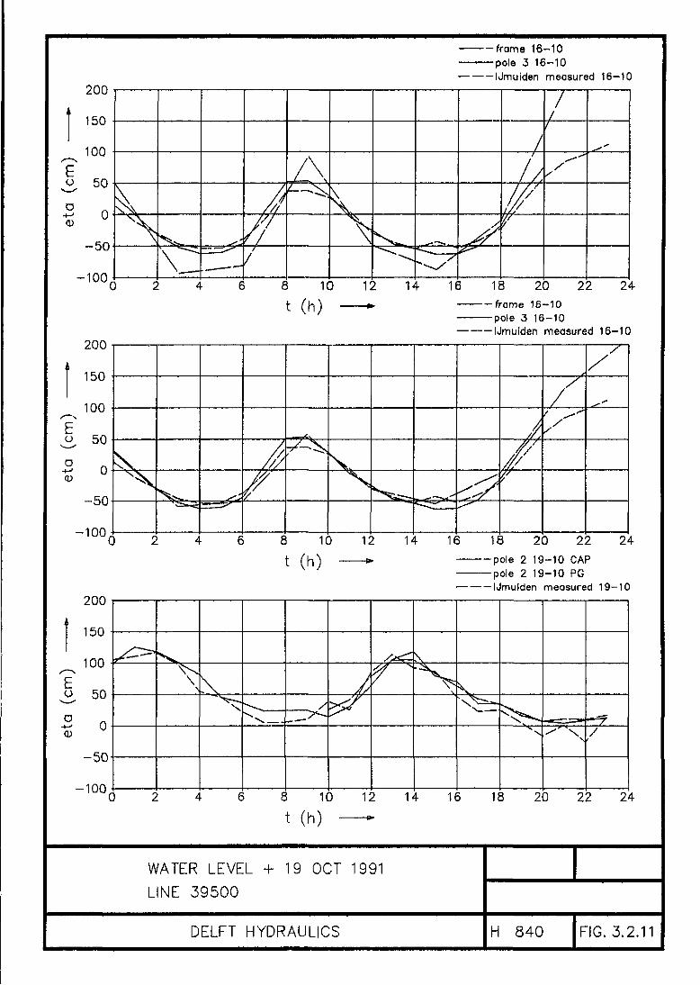
200
150
o 50
o 0
- 5 0
-100
200
150
o 50
a>
- 50
-100
200
150
100
o 50
- 5 0
-100
frame 16-10———pole 3 16-10
Umuiden measured 16-10
— -
/ //
V/
//V
If
\
0
8 10
(h)12 14 16 18 20 22 24-
—»• frame 16-10pole 3 16-10Umuiden measured 16-10
0 2
V-
I
™——-1"
6 £
\
10 12 U\ M
//,
5 18 20 22 24
t (h) • pole 2 19-10 CAPpole 2 19-10 PGIJmuiden measured 19-10
Y
•s N
8 10 12 14 16 18 20 22 24
t (h)
WATER LEVEL + 19 OCT 1991
LINE 39500
DELFT HYDRAULICS H 840 FIG. 3.2.11

CAP_ PG
200
150
100
o
D-t-J
£u
-100
-150
-200
200
150
100
50
0
-50
-100
-150
-2000
200
-200
longshore velocity
10 20
t (s)40 50 60
•cross—shore velocity
SURFACE ELEVATION + ORBITAL VELOCITIES
POLE 2, 15 H, 19-10-1991
DELFT HYDRAULICS H 840 FIG. 3.2.12

*Eu
Z
13
17
16
15
14
1 3 •
12
10
9 •
7 •
O 6
5 •
3 •
1 •
0.Q00 0.135 0.270 0.405 0.640 0,675 0.810 0.945 1.080 1.215 1.350 1.4B5 1.620 1.755 1.890 2.025
FREQUENCY (HZ)
= 2.73 ,n 3 cm«+2
tVM0 -
Tp =
NY ~
DF =
EDF =Pole 2,15 h, 19-10-1
ZUO.O I
16.00
2.0000
0,0078
72991, CAP
cm
S
HZ
HZ
ENERGY DENSITY SPECTRUM
DELFT HYDRAULICS H 840 FIG.3.2,13

17 -
^ 15 -
14 -
13 •
12 -m•
Csl# 11 ••eo
•*—* 1 0 •
9 -
»^_ it .
isin
O
O 6 •
Ixl
UJ a ,
4 .
3 -
2 .
1 •
0.000
t1 . M
rl vv y vA /W
v\ \V 1MA.
•
•
•
•
•
•
•
s
0.135 0.270 0.405 O.S40 0.675 0,810 0.945 1.08Q 1.215 1.350 1.485 1.620 1.755 1.890 2.026
4VM0 =
TP -FNV =
DF
EDF =
FREQUENCY (HZ)
5.62 10 3 cni»2
299.78 cm
14.22 s
2.0000 HZ
0.0078 HZ
60Pole 2, 15 h, 19-10-1991, EMS-x
ENERGY DENSITY SPECTRUM
DELFT HYDRAULICS
1
H 840 | F I G . 3 . 2 . 1 4
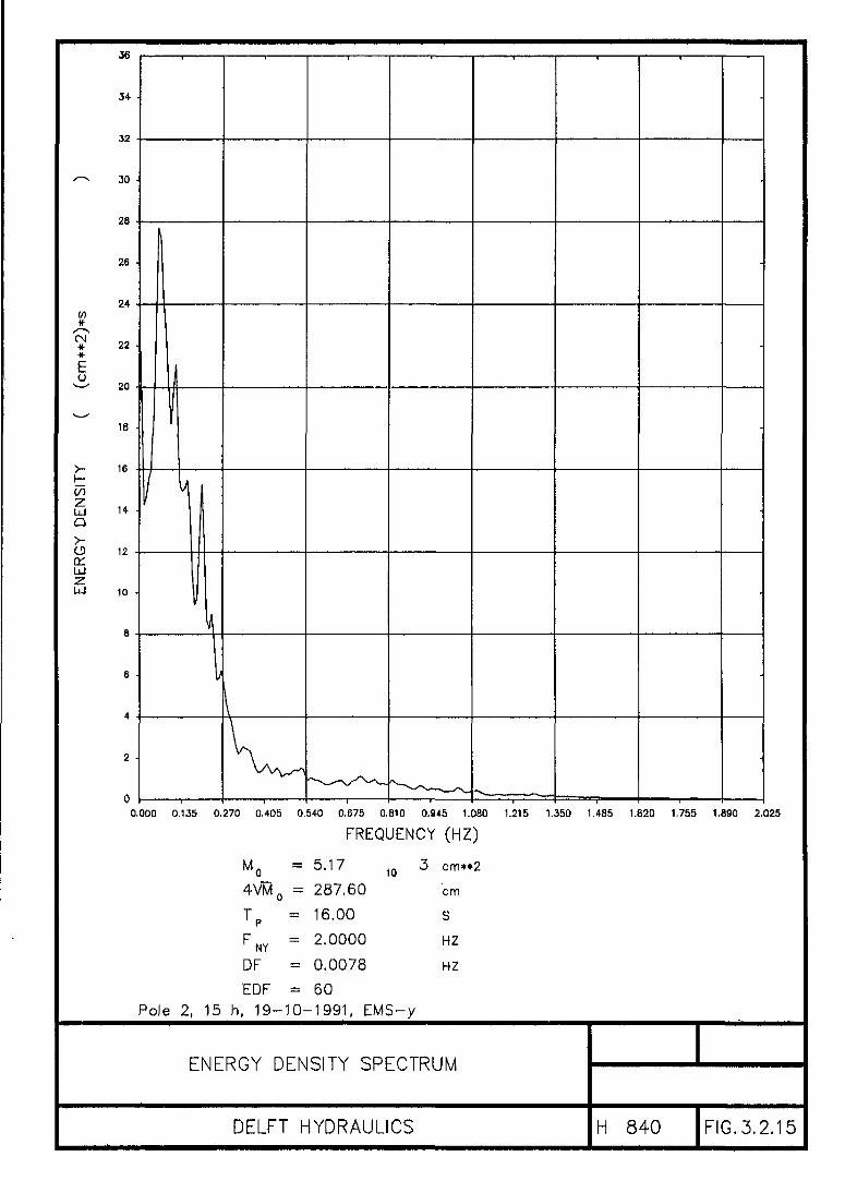
#
*
Eo
UJQ
a:UJ
UJ
28
26 •
22
20
18 •
>- 16
14
12
,0
0.000 0.135 0.270 0.405 0.540 0.675 0.B10 0.945 1.080 1.215 1.350 1.485 1.820 1.755 1,890 2.025
FREQUENCY (HZ)
3 cm+*2
cm
S
HZ
DF = 0.0078 HZ
EDF = 60Pole 2, 15 h, 19-10-1991, EMS-y
M = 5.17
4VM0 = 287,60
Tp = 16.00
FNy = 2.0000
ENERGY DENSITY SPECTRUM
DELFT HYDRAULICS H 840 lFIG.3.2.15

- 5 0
- 2 5
CO
o
3 0
25
50- 50 -25 0 25
v (cm/s)50
CORRELATION DIAGRAM
POLE 2, VELOCITIES NOVEMBER 1991
DELFT HYDRAULICS H 840 lFIG.3.2.16
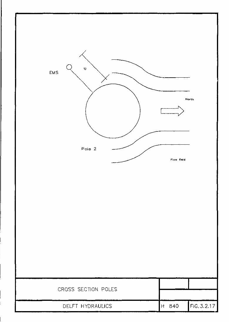
EMS
Pole 2
North
Flow field
CROSS SECTION POLES
DELFT HYDRAULICS H 840 FIG.3.2.17

JQN
2
0
- 2
- 4
- 6
- 8
-10-
-12
-14
-16
-18-
-13-09-1991
101000 101500
x (m) —102000 102500
29-10-1991
101000 101500
x (m) —102000 102500
13-09-199129-10-1991
101000 101500
X ( m ) —
102000 102500
ECHO SOUNDINGS
LINE 39500
DELFT HYDRAULICS H 840 FIG. 3.3.1

•11-1C-1991
0 -
E - 2
-QN
- 4 -
102600 102650
x (m)102700 102750 102S00
H-10-1991
0
E - 2 -
-ON
- 4 -
0-
E - 2
N
- 4 -
102600
102600
102650
x (m)102700 ' 102750
102650
x (m)102700
102800
11-10-1991H-10-1991
102750 102800
SAP BOTTOM PROFILES
LINE 39500
DELFT HYDRAULICS H 840 FIG. 3.3.2

-14-10-1991
0
E -2 -
X)N
2 T
102600 102650x (m)
102700 102750 102800
•23-10-1991
0-
E -2-
N
102600 102650x (m)
102700 102750 102800
• 14-10-199123-10-1991
0
E -
XIN
- 4 -
102600 102650
x (m)102700 102750 102800
SAP BOTTOM PROFILES
LINE 39500
DELFT HYDRAULICS H 840 FIG. 3.3.3

0
E - 2
N
- 4
E - 2
N
- 4
0-
E - 2
N
102600
102600
102600
102650
x (m)
102700
102650
x (m)
102700
102650x (m)
102700
-23-10-1991
102750 102800
-30-10-1991
102750 102800
23-10-199130-10-1991
102750 102800
SAP BOTTOM PROFILES
LINE 39500
DELFT HYDRAULICS H 840 FIG. 3.3.4

-30-10-1991
0
E -2
-QN
-4
102600 102650
x (m)102700 102750 102800
-01 — 11—1 &91
E -2
£1N
-4
102600 102650
X (m)
102700 102750 102800
30-10-199101-11-1991
0
E -2
N
-4-
102600 102650
x (m)102700 102750 102800
SAP BOTTOM PROFILES
LINE 39500
DELFT HYDRAULICS H 840 FIG. 3.3.5

NON UNIQUENESS OF THE SEDIMENT TRANSPORTFIELD AS DERIVED FROM TOPOGRAPHICCHANGES ONLY
DELFT HYDRAULICS H 840 FIG. 4.3.1

InputCondltios
wave heightwave periodwovedirection
water leveltidal current
Bottomprofile
Velocity alongbottom profile
Sediment trans-port rates
Bottomchanges
FLOW DIAGRAM UNIBEST-TC
DELFT HYDRAULICS H 840 FIG. 5.1.1

— CAP— PG
100
75
O
0)
-75
-100 0
longshore velocity
m
Eu
100
75
50
25
en
o
-25
-50
-75
-100,
100
75
50
25
A r\J \J V,A r \r\ A
V ^
10 20
t (s)30 40 50 60
-cross—shore velocity
..A-25-
1 - 5 0 ,
-75j
-100 j
\
Ivz
10
\ _r\
20t (s)
30 40 50 60
SURFACE ELEVATION + DEPEAKED VELOCITIES
POLE 3, 00 H, 16-10-1991
DELFT HYDRAULICS H 840 FIG. 6.2.1

CAPpG
100
75
o
o
-75
-1000
longshore velocity
CO
o
100
75
50
25
0
-50
-75
-100
A r\' \J v
A rk v/ V v
L/V Av y -> •
0 10 20
t (s)30 40 50 60
•cross-shore velocity
CO
Eo
100
75
50
25
•251 - 50
-75
-100
. A / \r \J1
\
Wy \V
A/ \ A -
\ /V
s / \ jv \ f
\J
\— \ /
V
0 10 20
t (s)30 40 50 60
SURFACE ELEVATION, DEPEAKED +FILTERED VELOCITIESPOLE 3, 00 H, 16-10-1991
DELFT HYDRAULICS H 840 FIG. 6.2.2

IRfift
3+00 -
^ 3000 •
9 an A
2600 •
Sf 2200 •
Eo
1S00 -
DE
NS
ITY
o
o
O 1200 -
LJ
zUJ 1000 •
flrtrt ,
600 •
400
200 •
i
1
u
1
\
V
•
•
•
•
•
0.000 0.135 0.270 0.405 0.S40 0.675 0.B10 0.945 1.080 1.215 1.350 1.485 1.620 1.755 1.890 2.025
FREQUENCY (HZ)
Mo = 249,13 cm**2
4VMQ = 63.14 cm
Tp = 0.00 S
FNY = 2.0000 HZ
DF = 0.0078 HZ
EDF = 72Pole 3, 00 h, 16-10-1991, CAP
ENERGY DENSITY SPECTRUM
DELFT HYDRAULICS H 840 FIG. 6.2.3

6500
HOOO
*—* 7500 -
6500 •
*
M 5500 •
o••*-** 5 0 0 0 •
4500 •
—
5 3500 •
aO 3000 •DCJj
U 2500 •
2000 •
1500 -
1000 •
500 •
0
II
J x
••
•
•
0.000 0.135 0.270 0.405 0.540 0.675 0.810 0.945 1.080 1.21S 1.350 1.485 1.620 1.755 1,890 2.025
FREQUENCY (HZ)
4VMQ =
TP -
DF =
EDF =
247.7262,96
6.74
2.0000
0.0078
60Pole 3, EMS-x, 16-10-1991, 00 h
(cm/s)*+2
cm/s
S
HZ
HZ
ENERGY DENSITY SPECTRUM
DELFT HYDRAULICS H 840 FIG. 6.2.4

ison
1700 •
1600
<--* 1500 •
1300 •
V)
A taoo •CM*
W 1100 •
Eo\ s 1000
900 •
(—</)
Q
>-O 600 •
rrLJJ•z.UJ 500 •
400 -
300 -
200 -
100 •
0
o.c
F
Ir
r
-
•
-
•
00 0.135 0.270 0.405 0.540 0.675 0.810 0.945 1.080 1.215 1.350 1.485 1.620 1.755 1.890 2.025
FREQUENCY (HZ)
Mo = 89.28 (cm/s)+*2
4VM0 = 37.79 cm/s
Tp - 6.74 s
FN¥ - 2.0000 HZ
DF = 0.0078 HZ
EOF = 60>o!e 3, EMS-y, 16-10-1991, 00 h
ENERGY DENSITY SPECTRUM
DELFT HYDRAULICS
IH 840 | R G . 6.2.5

200
150
100
eoDCO-100
-150
-200
200
150
100
50
o-50
'-100
-150
-2000
200
150
100
50
o-50
'-100
-150
-200
CAPPG
X
o
10
1
10
longshore velocitv
A JA\l\ -1
\A ,!
v v v
\
\ \ /\ 1
V
1rJ
\ /v
A A AA/v1
20
t (s)30 40 50 60
•cross—shore velocity
AV
7\
20t (s)
40
\J
50 60
SURFACE ELEVATION + CORRECTED VELOCITIES
POLE 2, 15 H, 19-10-1991
DELFT HYDRAULICS H 840 FIG. 6.2.6
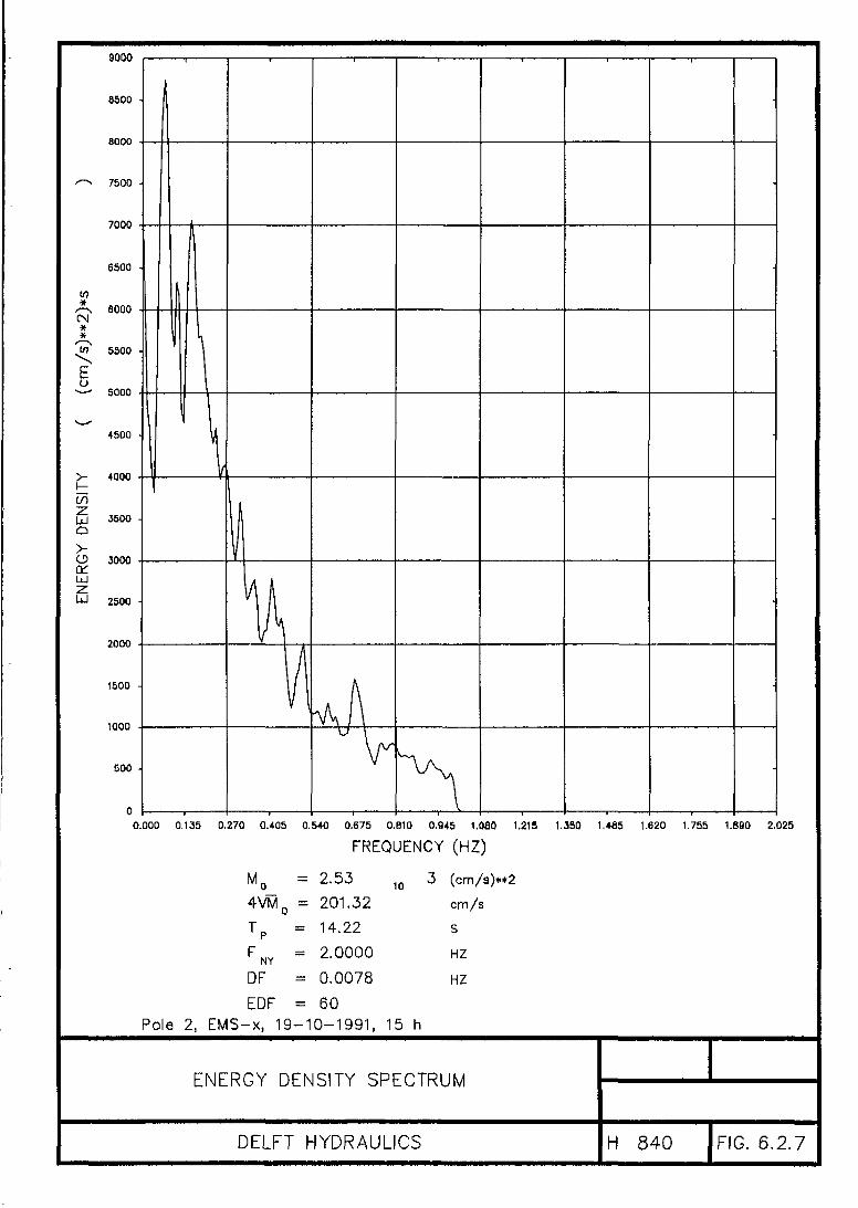
m
*
9000
6500 -
eooo
7500 -
7000
6500
eooo
tn 5500 •
osooo
+500
4000
t/1
UJQ
>-
ocUJz:UJ
3500
J00O
2500
2000
1500 •
tooo
500
0.000 0.135 0.270 0.405 0.540 0.675 0.B1Q 0.945 1,080 1.215 1.350 1.488 1.620 1.755 1.890 2.025
FREQUENCY (HZ)
Mn = 2.534VM0 = 201.32
10 3 (cm/s)++2
cm/s
Tp = 14.22 S
FNy = 2.0000 HZ
DF = 0.0078 HZ
EDF = 60Pole 2, EMS-x, 19-10-1991, 15 h
ENERGY DENSITY SPECTRUM
DELFT HYDRAULICS H 840 FIG. 6.2.7

*#,—*s
CO
Eo
CO
UJQ
)oa:
34 •
32 '
30 -
OR ,
ze -
24 •
22 -
18 -
1 f i •
1 4 •
12 •
to •
8 •
6 •
2 -
0
1
1
L1/ V1
1
1V —"-————-,
-•
•
•
•
-
•
0.000 0.135 0.270 0.405 0.540 0.675 0.810 0.945 1.080 1,215 1.350 1.485 1.620 1.755 1.890 2.025
MQ =
4VM0 =
Tp
OF =
FREQUENCY
4.79 ,0 3276.8616.002.0000
0.0078
(HZ)
(cm/s)++2
cm/s
S
HZ
HZ
EOF = 60Pole 2, EMS-y, 19-10-1991, 15 h
ENERGY DENSITY SPECTRUM
DELFT HYDRAULICS H 840 FIG. 6.2.8

125
100
75
50
25
0
- 2 5
50
25
- 5 0
-75
- 1 0
•^ frameX pole 3
"-8,25 -0.12 0.00 0.12 0.25 0.37 0.50 0.63 0,75 0.88 1.00
t (days)•t frameX pole 3
-%.25 -0.12 0.00 0.12 0.25 . 0.37 0.50 0.63 0.75 0,88 1,00t (days)
POLE 3 + FRAME, CURRENT VELOCITIES
17 H 15-10 TO 21 H 16-10
DELFT HYDRAULICS H 840 FIG. 6.2.9

+• frame
- 5 0
- 2 5
o
0
25
50- 5 0 - 2 5
-50
1 -25
3 0
25
50
0 25
v (cm/s)
- 50 - 2 5 0 25v (cm/s)
50 75 100
X pole 3
x# X X *
XX
X
50 75 100
CORRELATION DIAGRAM
VELOCITIES 16-10-1991
DELFT HYDRAULICS H 840 FIG.6.2.10

E
0 0. 2 0.'% O.f3 O.i3 1.0
15
10
CO
^ 5
8.
90
| 60
30en
- 6 0
0.2
0.2
t (days)
0.4
t (days)0.6
0.4
t (days)0.6
0.8
0.8
1.0
1.0
Hrms, Tp, DIR
LINE 39500 RUN ID.:H1
DELFT HYDRAUUCS H 840 FIG. 6.3.1

CO
Ex
8.
V v
15
10
V)'
A 5
8.
90
(de
gj
dir
60
30
0
- 3 0
- 6 0
-9D
0.2
0.2
0.2
0.4
t (days)0.6
0.4
t (days)0.6
0.4
t (days)0.6
0.8
0.8
0.8
1.0
A V1.0
1.0
Hrms, Tp, DIR
LINE 39500 RUN ID.:H2
DELFT HYDRAULICS H 840 FIG. 6.3.2

CO
as-
15
I -CO
,a 5
8.
90
60
30
0eCD
£ -30
-60
- 9.0
0.5
0.5
0.5
1.0 1.5
t (days) —
1.0 1.5
t (days) -
2.0
2.0
1.0 1.5
t (days) -2.0
2.5
2.5
3.0
3.0
A/ ^
A/
2.5 3.0
Hrms, Tp, DIR
LINE 39500 RUN ID.: Ml
DELFT HYDRAULICS H 840 FIG. 6.3.3

CO
E
enT3
90
60
30
0
;b - 3 0
- 6 0
- 9
8.0 1.0 2,0 3.0 4.0 5.0 6.0 7.0 8.0 9.0
t (days)
0 1.0 2.0 3.0 4.0 5.0 6.0 7.0 8,0 9.0
9.0 1.0 2.0 3.0 4.0 5.0 6.0 7.0 8.0 9.0
t (days)
Hrms, Tp, DIR
LINE 39500 RUN ID.:M2
DELFT HYDRAULICS H 840 FIG. 6.3.4
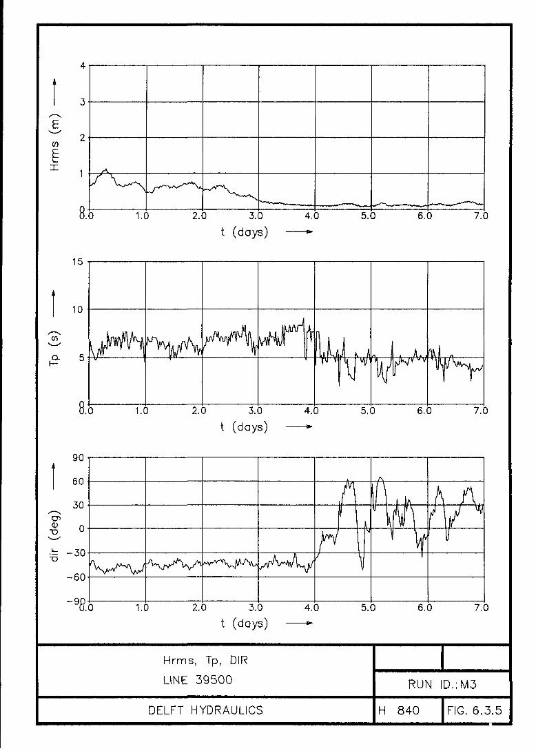
in
E/A
15
10
1.0
1.0
2.0 3.0
t (days)4.0
2.0 3.0 4.0
t (days) *•
2.0 3.0
t (days)
5.0
5.0
6.0
6.0
7.0
7.0
Hrms, Tp, DIR
LINE 39500 RUN ID.:M3
DELFT HYDRAULICS H 840 FIG. 6.3.5
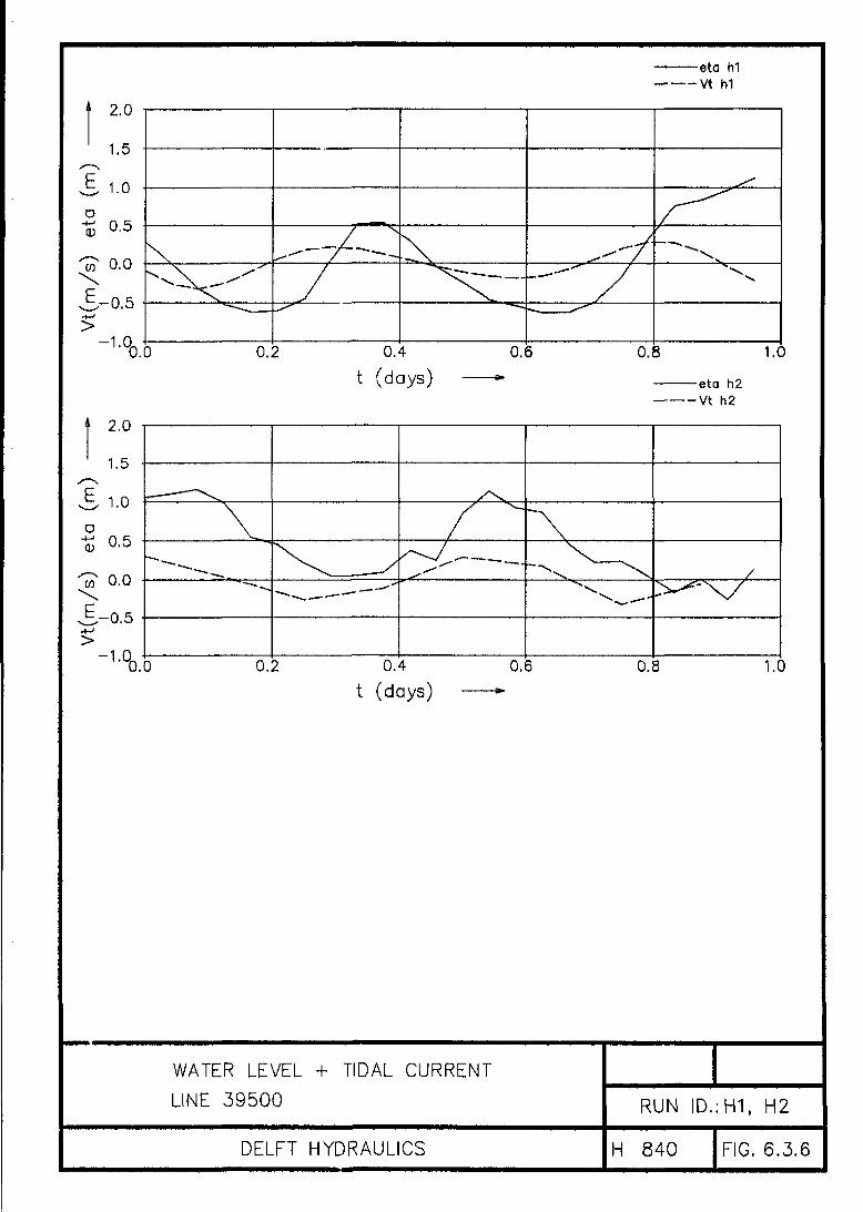
2.0
1.5
1.0
0.5
0,0
E_ 0.5
-1,0,0.0
D
2.0
1.5
1.0
0.5
1Z o.o1-0.5
- 1 .
• eta hiVt hi
0.2 0.4
t (days)0.6 0.8 1.0
eta h2Vt h2
0.2 0.4
t (days)0.6 0.8 1.0
WATER LEVEL + TIDAL CURRENT
LINE 39500 RUN ID.:H1, H2
DELFT HYDRAULICS H 840 FIG. 6.3.6

-—• ota mlVt ml
2.0
1.5
E 1.0
<U « •0,5
0.0
"-0.5
-1
-J
J
& ftV || \]\j \j V
fta ftV
0.0 1.0 2.0 3.0 4.0 5.0 6.0 7.0 8.0 9.0
t (days) » eta m2vt m2
0.0 1.0 2.0 3.0 4.0 5.0 6.0 7.0 8.0
-0.5
-1
eta m3Vt m3
0.0 1.0 2.0 3.0 4.0 5.0 6,0 7.0 8.0 9.0
WATER LEVEL + TIDAL CURRENT
LINE 39500 RUN ID.:M1, M2, M3
DELFT HYDRAULICS H 840 FIG. 6.3.7

I
c\|
oQ.
1!oa
o1—
CM
ooo1—•
ToT
oa
es(UoQ .
oom
x
oIN
O 00
[uu] qz [HI] qz
COMBINED BOTTOM PROFILE
LINE 39500
DELFT HYDRAULICS H 840 FIG. 6.3.8

I a.o
toCM
.4)O
0)
D
<P"5a
oIT)CM
Ooo
a0
oo
o
CM
[UJ] qz
CM
T
COMBINED BOTTOM PROFILE
LINE 39500
DELFT HYDRAULICS H 840 FIG. 6.3.9

Time seriesvelocities
correction
Ulo, Vic-
Time series
waves
Wave energyspec, fpass
Ulo.VIo
GOLANA
demean
filter fortidalHarmonics
FLOW DIAGRAM DATA PROCESSING
DELFT HYDRAULICS H 840 FIG. 6.4.1

<>—J o
/ Mean wave direction
/ v
u
DEFINITION VELOCITIES AND MEAN WAVE DIRECTION
DELFT HYDRAULICS H 840 FIG. 6.4.2

pole 3 PGpole 3 CAPmode!
£
2.50
2.00
1.50
1.00
0.50
0.
— ~z._—^
A
.000 0.125 0.250 0.375 0.500 0.625 0.750 0.875 1.000
T (days)framemodel
V)
E
2.50
2.00
1.50
1.00
0.50
0'°6°000 0,125 0.250 0.375 0.500 0.625 0.750 0,875 1,000T (days) "
Hrms
16-10-1991
DELFT HYDRAULICS H 840 FIG. 7.2.1

CO
£
2.50
2.00
1.50
1.00
0.50
2.50
2.00
1.50
1.00
0,50
pole 2 PGpole 2 CAPmodel
0.125 0.250 0.375 0.500 0.625T (days) *•
0.750 0.875 1.000
framemodel
O.QtP.000 0.125 0.250 0,375 0.500 0.625 0.750 0.875 1.000
T (days)
Hrms
19-10-1991
DELFT HYDRAULICS H 840 FIG. 7.2.2

90.00
-60.00
-90 .^ 0 0 0 0.125 0.250 0.375 0.500 0.625 0.750 0,875 1.000
T (days)
90.00
60.00
en
"^30.00
0.00
-30.00
-60.00
"9O'^£oOO 0.125 0.250 0.375 0.500 0.625 0.750 0.875 1.000
T (days) »
WAVE DIRECTION W.R.T. C.N.
16-10-1991
DELFT HYDRAULICS H 840 FIG. 7.2.3
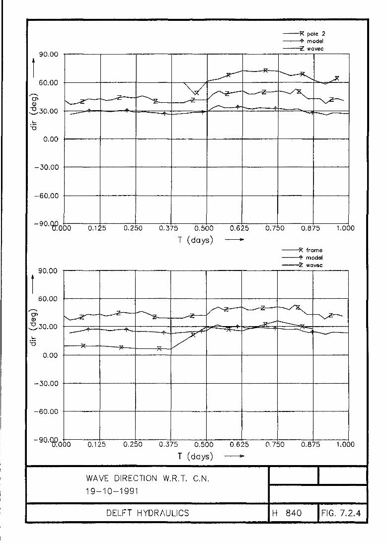
90.00
60.00
S-30.00
0.00
-30.00
-60.00
-90 .
T (days)
90.00
-90 .
pole 2modelwavec
:000 0,125 0.250 0.375 0.500 0.625 0.750 0.875 1.000
0.125 0.250 0.375 0.500 0.625 0.750 0.875 1.000
T (days) «-
WAVE DIRECTION W.R.T. C.N.
19-10-1991
DELFT HYDRAULICS H 840 FIG. 7.2.4

0.12
0.00
-0.37
-0.50
-0.63
-0.75
-0.88
-1.0,
0.12
0.00
- 0 . 1 2
j=- 0.25
^ - 0 . 3 7
0.50
0.63
0,75
0.88
-1.Q
pole 3model
#000 0.125 0.250 0.375 0.500 0.625
T (days) -0.750 0.875
•framemodel
1.000
$000 0.125 0.250 0.375 0.500 0,625
T (days) -0.750 0.875 1.000
RETURN VELOCITY
16-10-1991
DELFT HYDRAULICS H 840 FIG. 7.2.5

pole 2model
0.25
0.12
0.00
-0.25
-0.37
-0.50
-0.63
-0.75
-0,88
•RSooo
... f-____. if1—
-"—5S-
T1
,* 5!
t
0.25
0.12
0.00
s-0.12
-0.25
-0,37
-0.50
-0,63
-0.75
-0.88
-1,0,
0.125 0.250 0.375 0.500 0.625 0.750T (days)
0.875
framemodel
1.000
$000 0.125 0.250 0.375 0.500 0,625
T (days)0,750 0.875 1.000
RETURN VELOCITY
19-10-1991
DELFT HYDRAULICS H 840 FIG. 7.2.6

pole 3model
2.00
1.50
E 1.00
0.50
0.00
0.50
2.00
1.50
0.50
0.00
-0.50
0.125 0.250 0.375 0.500
T (days)0.625 0.750 0.875 1.000
framemodel
,000 0.125 0.250 0.375 0.500 0.625 0.750 0.875 1.000
T (days) -
LONGSHORE VELOCITY
16-10-1991
DELFT HYDRAULICS H 840 FIG. 7.2.7

2.00
1.50
In 1.00
E^ 0.50>
0.00
-0.50
-1.00
-1.50
-2.0JD,
2.00
1.50
1.00
0.50
0.00
-0.50
-1,00
-1.50
-2.0^0
pole 2model
'ffoOO 0.125 0.250 0.375 0.500 0.625 0.750 0.875 1.000
T (days) »•framemodel
A
%°000 0.125 0.250 0.375 0.500 0.625 0.750 0,875 1.000
T (days)
LONGSHORE VELOCITY
19-10-1991
DELFT HYDRAULICS H 840 FIG. 7.2.8
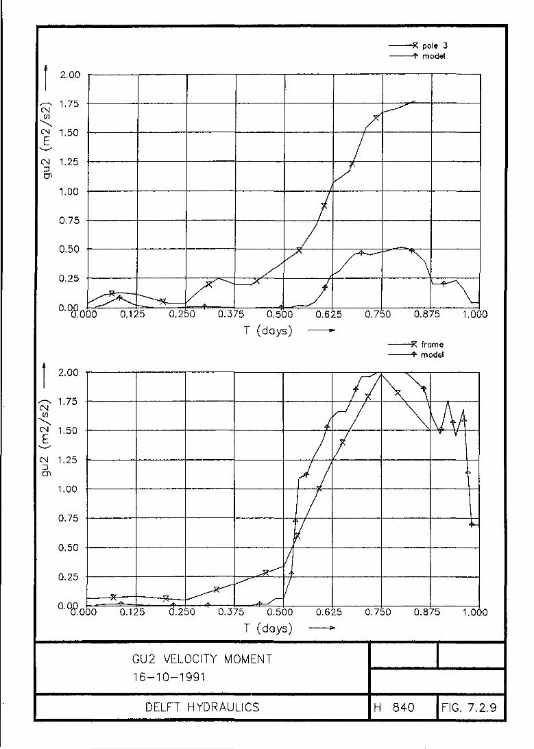
CMCO
2.00
1.75
1.50
CM 1.25
1.00
0.75
0.50
0.25
ao6°ofcf
CM
2.00
1.75
1.50
CM 1,25
en
1.00
0.75
0.50
0,25
ao6°ooT
pole 3model
0.125 0.250
1
0.375 0.500
T (days)
0.625 0.750 0.875
framemodel
1.000
0.125 0.250 0.375 0.500 0.625 0,750 0.875 1.000
T (days)
GU2 VELOCITY MOMENT
16-10-1991
DELFT HYDRAULICS H 840 FIG. 7.2.9

pole 2model
CO
CN
CN
3.00
2.75
2.50
2,25
2.00
1.75
1.50
1.25
1.00
0.75
0.50
0.25
0.°(SoOO 0.125 0.250 0.375 0.500
T (days)0,625 0.750 0.875
framemodel
1.000
CMV)
CN 2
CN
cn
O.QC0.125 0.250 0.375 0.500
T (days)0.625 0.750 0.875 1.000
GU2 VELOCITY MOMENT
19-10-1991
DELFT HYDRAULICS H 840 FIG.7.2.10

pole 3model
3.00
to
E2.00
1.50
1.00
0.50
rototo£
3.00
2,50
2.00
1.50
1.00
0.50
0.125 0.250 0.375 0.500
T (days)0.625 0.750 0.875 1.000
framemodel
°'°6300O 0.125 0.250 0.375 0.500 0.625 0.750 0.875 1.000
T (days) *•
GU3 VELOCITY MOMENT
16-10-1991
DELFT HYDRAULICS H 840 FIG. 7.2.11

pole 2model
ro
roE
en
5.00
4.00
3.00
2.00
1.00
0,°8,000 0.125 0.250 0,375 0.500 0.625 0.750 0.875 1.000
T (days) *•framemodel
roCO
roE
CD
5.00
4.00
3.00
2.00
1.00
°'06°000 0.125 0.250 0.375 0.500 0.625 0.750 0.875 1.000
T (days) •>
GU3 VELOCiTY MOMENT
19-10-1991
DELFT HYDRAULICS H 840 FIG.7.2.12
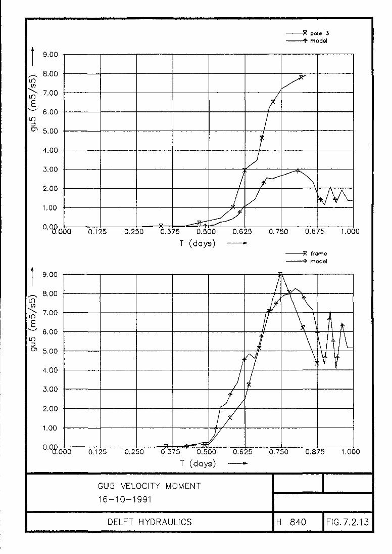
pole 3model
3
9.00
8.00
6.00
5.00
4.00
3.00
2.00
1.00
0.Q
i n
LO3
9.00
8.00
7.00
6.00
5.00
4.00
3.00
2,00
1.00
0.0,
0.125 0.250 0.375 0.500
T (days)0.625 0.750 0.875 1.000
framemodel
0.125 0.250 0.375 0.500 0.625 0.750 0.875 1.000
T (days) «*
GU5 VELOCITY MOMENT16-10-1991
DELFT HYDRAULICS H 840 FIG.7.2.13

pole 2model
15.00
LO
\12.00LO
E
9.00
6.00
3.00
°'O(SoOO 0.125 0.250 0.375 0,500 0.625 0.750 0.875 1.000
T (days) <*•framemodel
°'00°000 0.125 0.250 0.375 0.500 0.625 0.750 0.875 1.000
T (days) <*•
GU5 VELOCITY MOMENT
19-10-1991
DELFT HYDRAUUCS H 840 FIG.7.2.14

CO
0.50
0.00
X
-0.50
-1.00
-1.50
- 2 .
V)
0-50
0.00
^ - 0 . 5 0en
-1.00
-1.50
pole 3model
1 7 T ^
0.125 0.250 0.375 0.500 0.625 0.750 0.875 1.000
T (days)framemodel
\
'Z(00000 0.125 0.250 0.375 0.500 0.625 0.750 0.875 1.000
T (days) -
GU2UX VELOCITY MOMENT
16-10-1991
DELFT HYDRAULICS H 840 FIG.7.2.15

pole 2model
1.00
0.50X13
CN
0.00
-0.50
\
V
1'°0°000 0.125 0.250 0,375 0,500 0.625 0.750 0.875 1.000
framemodel
1.00
CO
xCN
cn
0.50
0.00
-0.50
^X7
"1lC(fio0O 0.125 0.250 0.375 0.500 0.625 0.750 0.875 1.000
T (days) <*
GU2UX VELOCITY MOMENT
19-10-1991
DELFT HYDRAULICS H 840 FIG. 7.2.16

ro
CM
2.50
2.00
1-50
1.00
0.50
0.00
0.125 0.250 0.375 0.500T (days)
O250T (days)
pole 3model
0.625 0.750 0.875 1.000
framemodel
0.750 0.875
GU2UY VELOCITY MOMENT16-10-1991
DELFT HYDRAULICS H 840 FIG.7.2.17

pole 2model
0.00
en
£-1.00
3en
-2.00
-3.00
- 4 . OP.7000 0.125 0.250 0.375 0.500 0,625
T (days) —~0.750 0.875 1.000
framemodel
0.00
ro
,-1.00
3
-2.00
-3.00
- 4 . OP.%°000 0.125 0.250 0.375 0.500 0.625 0.750 0,875 1.000
T (days)
GU2UY VELOCITY MOMENT
19-10-1991
DELFT HYDRAULICS H 840 lFIG.7.2.18

pole 3model
CO\
£
0.50
0.00
xCO
CD
-0,50
-1.00
-1.50
- 2 .
* — £ .
?(?000 0.125 0.250 0.375 0.500 0.625
T (days)0.750 0.875 1.000
framemodel
QCO
0.50
0.00
X
en-0.50
-1.00
-1,50
"2l<8?000 0,125 0,250 0.375 0.500 0.625 0.750 0.875 1.000T (days) •*•
SHORT-WAVE INTERACTION
16-10-1991
DELFT HYDRAULICS H 840 IFIG. 7.2.19

pole 2model
oCO
1.00
0.50
" 0.00
-0.50
-1.00
1<56°00O 0.125 0.250 0.375 0.500 0,625 0.750 0.875 1.000
T (days) — »framemodel
en
x
1,00
0.50
0.00
-0.50
-1.00
"1l56°OOO 0.125 0.250 0.375 0.500 0.625 0.750 0.875 1.000
T (days) *•
SHORT-WAVE INTERACTION
19-10-1991
DELFT HYDRAULICS H 840 FIG.7.2.20

pole 3model
ro
en
en
2,50
2.00
1.50
1.00
0.50
0.00 • * •
to
3en
2.50
2.00
1.50
1.00
0.50
0.00 - * -
°'%?000 0.125 0.250 0.375 0.500 0.625 0.750 0.875 1.000
T (days) *•framemodel
'°'%°000 0.125 0.250 0.375 0.500 0,625 0.750 0.875 1.000
T (days ) *•
SHORT-WAVE INTERACTION
16-10-1991
DELFT HYDRAULICS H 840 FIG. 7.2.21

ro
3en
2.50
2.00
1.50
1.00
0.50
0.00
- 0 .
coen
2.50
2.00
1.50
1.00
0.50
0,00
T (days)
pole 2model
" —— r V- • 5?-
——^Kv—
^-—• -X
"""""•""-•4*—-v.
~~-5i
7000 0.125 0.250 0.375 0.500 0.625 0.750 0.875 1,000
framemodel
"°"%°000 0.125 0.250 0.375 0.500 0.625 0.750 0.875 1,000
T (days) <-
SHORT-WAVE INTERACTION
19-10-1991
DELFT HYDRAULICS H 840 FIG.7.2.22
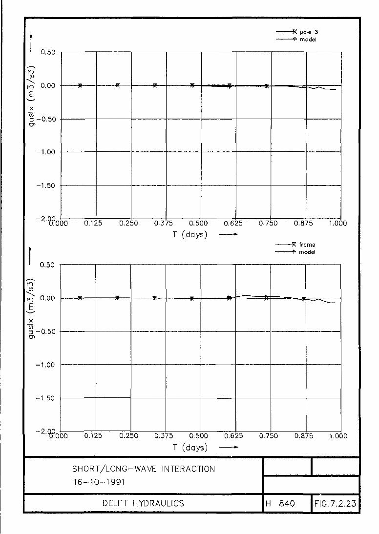
pole 3model
roV)
£,
en
0.50
0.00
-0.50
-1.00
-1.50
-2.QP.
-*- • * •
%°000 0.125 0.250 0.375 0.500 0.625 0.750 0.875 1,000
T (days)framemodel
E
en
0.50
0.00
-0.50
-1.00
-1.50
• * -
'2-{D0000 0.125 0.250 0.375 0.500 0.625 0.750 0.875 1.000
T (days) <-
SHORT/LONG-WAVE INTERACTION
16-10-1991
DELFT HYDRAULICS H 840 FIG.7.2.23
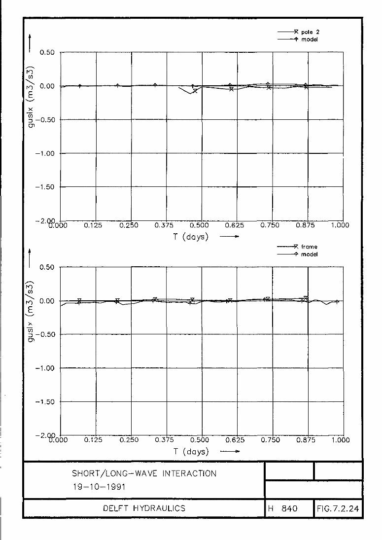
pole 2model
0.50
0.00
=3 - 0 . 5 0
-1.00
-1.50
- 2 .
I I • 1 " if- I
- — % -
• • • - f r . .
T000 0.125 0.250 0.375 0.500 0.625 0.750 0.S75 1.000
T (days)framemodel
0.50
0.00
-0.50
-1.00
-1.50
"2"%0000 0.125 0.250 0.375 0.500 0.625 0.750 0.875 1.000
T (days) — *
SHORT/LONG-WAVE INTERACTION
19-10-1991
DELFT HYDRAULICS H 840 FIG.7.2.24

roroE
CO3
2.50
2.00
1.50
1.00
0.50
0.00
- 0 .
fOCO
<n
2.50
2.00
1.50
1.00
0.50
0,00
-0.50
pole 3model
W , -
0.125 0.250 0,375 0.500 0.625 0.750 0.875 1.000T (days) ^
framemodel
V 1 g=^=—
%°000 0.125 0.250 0.375 0.500 0.625 0.750 0,875 1.000
T (days)
SHORT/LONG-WAVE INTERACTION16-10-1991
DELFT HYDRAULICS H 840 FIG.7.2.25

pole 2model
13
2,50
2.00
1.50
1.00
0.50
0.00
toin
COzs
2.50
2.00
1.50
1.00
0.50
0.00
T (days)
framemodel
°'%°000 0,125 0.250 0.375 0.500 0.625 0.750 0.875 1.000
T (days) **
=—^—. =—«== 8K— = - « n—n —
,000 0.125 0.250 0.375 0,500 0.625 0.750 0.875 1.000
SHORT/LONG-WAVE INTERACTION
19-10-1991
DELFT HYDRAULICS H 840 FIG.7.2.26

pole 3model
0.50
°-00
XuI -0.50
-1.00
-1,50
2>%°000 0.125 0.250 0.375 0.500
T (days)0.625 0.750 0.875 1.000
framemodel
CO
0.50
0.00
u1-0.50a*
-1.00
-1.50
• * • • * •
"2lC00000 0.125 0.250 0.375 0.500 0.625 0.750 0.875 1.000
T (days) *
WAVE-CURRENT INTERACTION
16-10-1991
DELFT HYDRAULICS H 840 FIG.7.2.27
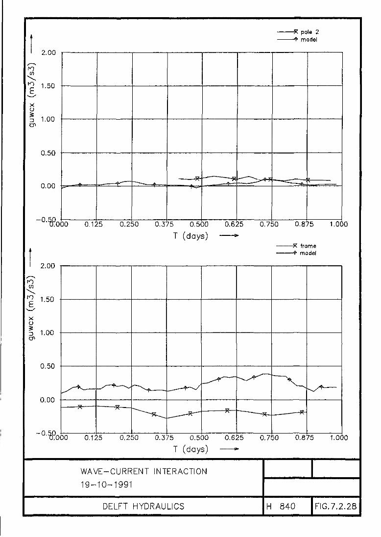
pole 2model
CO
2.00
1t5°xo3 1.00
0.50
0.00
"°"%°000 0,125 0.250 0.375 0.500 0.625 0.750 0.875 1.000
T (days) *•framemodel
2.00
£ 1'5°xoen
1.00
0.50
0.00
0.125 0,250 0.375 0.500 0.625 0.750 0.875 1.000
T (days) "-
WAVE-CURRENT INTERACTION
19-10-1991
DELFT HYDRAULICS H 840 FIG.7.2.28

I-O
2.50
2.00
1-50
1.00
0.50
0.00
- 0 . ffi
E
2.50
2.00
u1 1.50
1.00
0.50
0.00
000 0.125
pole 3rroclel
0.250 0,375 0.500
T (days)0.625 0.750 0.875 1.000
•-5? frame— ^ model
0.125 0.250 0.375 0.500 0.625 0.750 0.875 1.000T (days) «*
WAVE-CURRENT INTERACTION
16-10-1991
DELFT HYDRAULICS H 840 FIG.7.2.29

pote 2model
C/)
0.50
0.00
oI -0.50
-1.00
-1.50
2'%°000 0.125 0.250 0.375 0.500 0.625
T (days) "*0.750 0.875 1.000
framemodel
- 2 .).000 0,125 0.250 0.375 0.500 0.625 0.750 0.875 1.000
T (days) *•
WAVE-CURRENT INTERACTION
19-10-1991
DELFT HYDRAULICS H 840 lFIG.7.2.30

pole 3model
CO
nE
X
0.50
0.00
-0.50
-1.00
-1.50
- 2 .
to
r-o
Ex
0.50
0.00
-0.50
-1.00
-1.50
0.125 0.250 0.375 0.500 0.625 0.750 0.875 1.000
T (days) •-framemodel
• * -
'2-(00000 0.125 0,250 0.375 0.500 0.625 0.750 0.875 1.000
T (clays) »•
CURRENT iNTERACTION
16-10-1991
DELFT HYDRAULICS H 840 FIG. 7.2.31

pole 2model
CO
E
x
en
0.50
0.00
-0.50
-1.00
-1.50
- 2 .
w
7000 0.125 0.250 0.375 0.500 0.625 0.750 0.875 1.000
T (days) — *framemodel
-1.50
"2<(00000 0.125 0.250 0.375 0.500 0.625 0.750 0.875 1.000
T (days) — - *
CURRENT INTERACTION19-10-1991
DELFT HYDRAULICS H 840 FIG.7.2.32

pole 3mode!
ro
u=3
2.50
2.00
1.50
1.00
0.50
0.00
CO
CO
oen
2.50
2.00
1-50
1.00
0,50
0.00
T (days)
- 0 .
T (days)
framemodel
°'%°000 0.125 0.250 0.375 0.500 0.625 0.750 0.875 1.000
• 3 ?-3^
J /
1// X
7000 0.125 0.250 0.375 0.500 0.625 0.750 0.875 1.000
CURRENT INTERACTION
16-10-1991
DELFT HYDRAULICS H 840 FIG.7.2.33
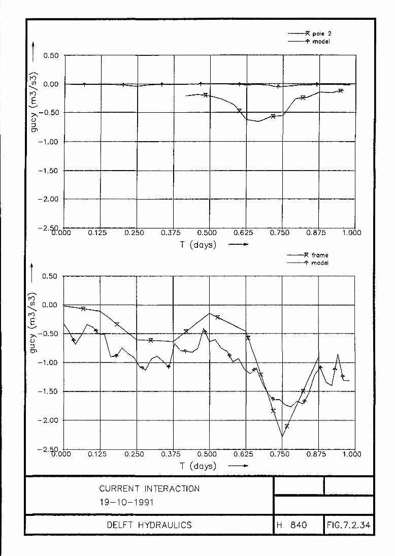
to
oCD
0.50
0.00
-0,50
-1.00
-1,50
-2.00
0.50
0.00rO
^ - 0 . 5 0
-1.00
-1.50
-2.00
V / \
pole 2model
"2'%°000 0.125 0.250 0.375 0.500 0.625 0.750 0.875 1.000
T (days) *•framemodel
"2'%°000 0.125 0.250 0.375 0.500 0.625 0.750 0.875 1.000
T (days) "
CURRENT INTERACTION
19-10-1991
DELFT HYDRAULICS H 840 FIG,7,2.34
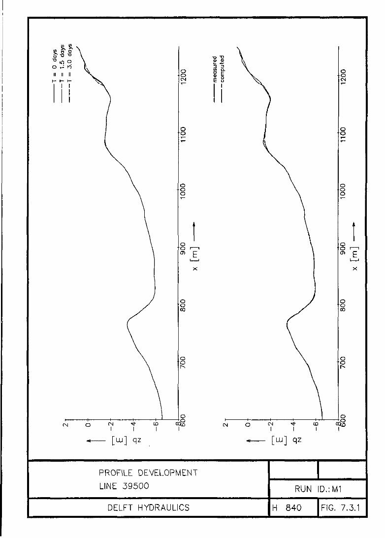
a.
8ooCM
OO
OOo
ooJ
[LU] qz [LU] qz
PROFILE DEVELOPMENT
LINE 39500 RUN ID.:M1
DELFT HYDRAULICS H 840 FIG. 7.3.1

Ei
X
[ U J ] qz [UJ] qz
PROFILE DEVELOPMENT
LINE 39500 RUN ID.:M2
DELFT HYDRAULICS H 840 FIG. 7.3.2

[w] qz [ai] qz
PROFILE DEVELOPMENT
LINE 39500 RUN iD.:M2
DELFT HYDRAULICS H 840 FIG. 7.3.3

[w] qz [LU] qz
PROFILE DEVELOPMENT
LINE 39500 RUN ID.:M3
DELFT HYDRAULICS H 840 FIG. 7.3.4

in w(^ o a
•° o oO Kl <*
II II IIt— t— 1—
11f
omoood
«•—
o
oood
o
oood
oCNOOod
/euu]
SEDIMENT
LINE
Is)
c
\
\
i
\
\
\
\
\
\
V\
\i
\
V\
\\
\
\
1i1
1iII .
a o o*— o *—o o 2o o go o 9d d o
doys
days
days
o o otri t& ai
oa ii it Hw i— 1—1—
1
iI
1100
1000
oO i 1
X
800
oo
oo ' "•
^ oi noood
• * -
TRANSPORT RATES
39500
DELFT HYDRAULICS
o
oood
(\
\
\
o
oood
/
/
//
/
(
\
1
oOOod
H
f
\ '
1 \\ !
Vi
1
1I
J/
\ \\\
1
ooood
] XS
RUN
840
nS 1
1//
/
O OO r-o o^ sD O
^ ?
ooCM
1100
1000
a
i
o i—>
X
800
oo
ooto
ID.:M2
FIG. 7.3.5

— [LU] qz
PROFILE DEVELOPMENT
LINE 39500
[ w ] qz
RUN ID.:M2S
DELFT HYDRAULICS H 840 FIG. 7.3.6
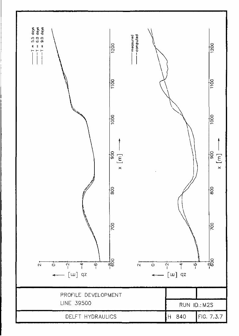
X
[ w ] qz
PROFILE DEVELOPMENT
LINE 39500 RUN ID.:M2S
DELFT HYDRAULICS H 840 FIG. 7.3.7

Appendix A
Third-order odd velocity constituents

Application-oriented validation of a cross-shore sediment transport model H 840 - June 1993
Given the third-order odd velocity moment in the cross-shore direction:
<w|wrz|> (al)
where:
«, = \ju2 + v2 (a2)
introducing in (a.l) before time-averaging:
u = u + u<a3)
v = v + {•
yields:
~ (it + tf)((« + ff)2 + <v + y>2)_ (a4)
•• w3 + iiv2 + 3MM2 + 3i?tf + MV2 + 2«vP + 2vM + fi3 + wv2
time averaging of (a.4) yields the following expressions for the velocity momentconstituents:constituents:
guc = u(j? + v2)
guwc = u(tf + v2) + 2MM2 + 2i?Pfi (a5)
gwu «
Introducing a short and long wave velocity component:
& = «, + M; (a6)
into the wave interaction term gww yields:
~ <«, + « , )«« ,+H,) 2 + (vs+v,)2)
/ / ? 2 + M;VS2 + (a7)
assuming that the long wave velocity is much smaller in magnitude than the short waveorbital velocity and time-averaging yields:
gus = M/M,2 + v,2)(a8)
gusl = * 2
delft hydraulics A — 1