DELFT UNIVERSITY OF TECHNOLOGY

REPORT 12-02

A Case Study in the Future Challenges in Electricity GridInfrastructure

Marjan van den Akker (Utrecht University),Herman Blok (University of Leiden),Chris Budd (University of Bath),Rob Eggermont (TU Eindhoven),

Alexander Guterman (Moscow State University),Domenico Lahaye (TU Delft) (corresponding author),Jesper Lansink Rotgerink (University of Twente),

Keith W. Myerscough (CWI Amsterdam),Corien Prins (TU Eindhoven),

Thijs Tromper (University of Twente),and Wander Wadman (CWI Amsterdam)

ISSN 1389-6520

Reports of the Department of Applied Mathematical Analysis

Delft 2012

Copyright 2012 by Department of Applied Mathematical Analysis, Delft, The Netherlands.

No part of the Journal may be reproduced, stored in a retrieval system, or transmitted, in anyform or by any means, electronic, mechanical, photocopying, recording, or otherwise, without theprior written permission from Department of Applied Mathematical Analysis, Delft University ofTechnology, The Netherlands.

A Case Study in the Future Challenges in Electricity Grid

Infrastructure ∗

Marjan van den Akker (Utrecht University),Herman Blok (University of Leiden),Chris Budd (University of Bath),Rob Eggermont (TU Eindhoven),

Alexander Guterman (Moscow State University),Domenico Lahaye (TU Delft) (corresponding author) †,

Jesper Lansink Rotgerink (University of Twente),Keith W. Myerscough (CWI Amsterdam),

Corien Prins (TU Eindhoven),Thijs Tromper (University of Twente),

and Wander Wadman (CWI Amsterdam)

Abstract

The generation by renewables and the loading by electrical vehicle charging imposes severechallenges in the redesign of today’s power supply systems. Indeed, accomodating these emerg-ing power sources and sinks requires traditional power systems to evolve from rigid centralizedunidirectional architectures to intelligent decentralized entities allowing a bi-directional powerflow. In the case study proposed by ENDINET, we investigate how the penetration of solarpanels and of battery charging stations on large scale affects the voltage quality and loss levelin a distribution network servicing a residential area in Eindhoven, The Netherlands. In ourcase study we take the average household load during summer and winter into account andconsider both a radial and meshed topology of the network. For both topologies our studyresults in a quantification of the levels of penetration as well as a strategy for electrical vehicleloading strategy that meet the voltage and loss requirements in the network.

Keywords: power systems, load flow computations, distributed generation, electrical ve-hicle charging

1 Introduction

The problem brought to SWI2012 by ENDINET is the hugely important question of the futureperformance, stability and integrity of the power supply network. The issues facing power gen-eration are changing rapidly. Until recently we have had a situation of a small number of largesuppliers of electricity (typically power stations delivering 100MW or more of power to consumerswith high demand during the day and low demand at night. In the future, and with the com-ming of the smart grid, this will change. In particular we will see a large number of small scalegeneration (and storage) of power (in the range of 1-10kW) from households, typically through

∗Problem contributed by ENDINET (www.endinet.nl, contact person: Sharmistha Bhattacharyya)†Delft University of Technology, Delft Institute of Applied Mathematics, Mekelweg 4, 2628 CD Delft, The

Netherlands. E-mail: d.j.p.lahaye@tudelft.nl

1

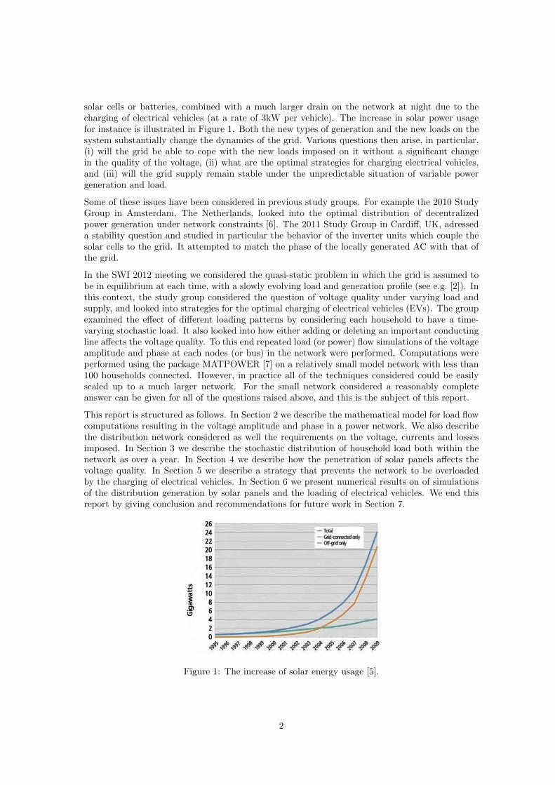
solar cells or batteries, combined with a much larger drain on the network at night due to thecharging of electrical vehicles (at a rate of 3kW per vehicle). The increase in solar power usagefor instance is illustrated in Figure 1. Both the new types of generation and the new loads on thesystem substantially change the dynamics of the grid. Various questions then arise, in particular,(i) will the grid be able to cope with the new loads imposed on it without a significant changein the quality of the voltage, (ii) what are the optimal strategies for charging electrical vehicles,and (iii) will the grid supply remain stable under the unpredictable situation of variable powergeneration and load.

Some of these issues have been considered in previous study groups. For example the 2010 StudyGroup in Amsterdam, The Netherlands, looked into the optimal distribution of decentralizedpower generation under network constraints [6]. The 2011 Study Group in Cardiff, UK, adresseda stability question and studied in particular the behavior of the inverter units which couple thesolar cells to the grid. It attempted to match the phase of the locally generated AC with that ofthe grid.

In the SWI 2012 meeting we considered the quasi-static problem in which the grid is assumed tobe in equilibrium at each time, with a slowly evolving load and generation profile (see e.g. [2]). Inthis context, the study group considered the question of voltage quality under varying load andsupply, and looked into strategies for the optimal charging of electrical vehicles (EVs). The groupexamined the effect of different loading patterns by considering each household to have a time-varying stochastic load. It also looked into how either adding or deleting an important conductingline affects the voltage quality. To this end repeated load (or power) flow simulations of the voltageamplitude and phase at each nodes (or bus) in the network were performed. Computations wereperformed using the package MATPOWER [7] on a relatively small model network with less than100 households connected. However, in practice all of the techniques considered could be easilyscaled up to a much larger network. For the small network considered a reasonably completeanswer can be given for all of the questions raised above, and this is the subject of this report.

This report is structured as follows. In Section 2 we describe the mathematical model for load flowcomputations resulting in the voltage amplitude and phase in a power network. We also describethe distribution network considered as well the requirements on the voltage, currents and lossesimposed. In Section 3 we describe the stochastic distribution of household load both within thenetwork as over a year. In Section 4 we describe how the penetration of solar panels affects thevoltage quality. In Section 5 we describe a strategy that prevents the network to be overloadedby the charging of electrical vehicles. In Section 6 we present numerical results on of simulationsof the distribution generation by solar panels and the loading of electrical vehicles. We end thisreport by giving conclusion and recommendations for future work in Section 7.

Figure 1: The increase of solar energy usage [5].

2

2 Power Flow Problem

The power flow problem is the problem to determine the voltage at each bus of a power system,given the supply at each generator and the demand at each load in the network (see e.g. [2]). Thenetwork we will consider is a low voltage network supplying a residential area consisting of a fewstreets. The power is fed into a network by a connection to medium voltage network through astransformer that can be regarded as an infinite source of power. The solar panels installed will betaken into account as decentralized power sources. Apart from the household loads, we will alsotake the loads of the charging of vehicles into account.

Let Y = G + jB denote the network admittance matrix of the power system. Then the powerflow problem can be formulated as the nonlinear system of equations∑N

k=1 |Vi| |Vk| (Gik cos δik +Bik sin δik) = Pi, (1)∑Nk=1 |Vi| |Vk| (Gik sin δik −Bik cos δik) = Qi, (2)

where |Vi| is the voltage magnitude, δi is the voltage angle, with δij = δi − δj , Pi is the activepower, and Qi is the reactive power at bus i. The current, voltage and power are measured inAmpere (A), Volts (V) and Watts (W), respectively. For details we refer to e.g. [2].

Define the power mismatch function as

~F (~x) =

[Pi −

∑Nk=1 |Vi| |Vk| (Gik cos δik +Bik sin δik)

Qi −∑N

k=1 |Vi| |Vk| (Gik sin δik −Bik cos δik)

](3)

where ~x is the vector of voltage angles and magnitudes. Then the power flow problem (1), (2) canbe reformulated as finding a solution vector ~x such that

~F (~x) = ~0. (4)

This is the system of non-linear equations that we solve to find the solution of the power flowproblem. In our experiments we will make use of the MATPOWER package [7].

In our study we perform repeated load flow computations to simulate the load profile over thecourse of a week in either summer or winter. We seek to understand to what extend the solarpanels can penetrate in the required power generation and to what affect the EVs can be loadedwith out introducing malfunctions in the network.

2.1 Distribution Network Considered

The distribution network considered is the network with 14 busses and 14 lines shown in Figure 2.It consists of two branches. The upper branch in this figure has a meshes structure as custumorsin this branch are fed from more than one source. The lower branch is intentionally kept radialto make the case study more interesting. The busses are numbered consecutively from 1 to 9 andfrom 10 to 14 by first traversing the upper and then the lower branch in from top left to bottomright. The dotted line in the lower right part of the figure is a hypothetical that ENDINETconsiders building to convert the radial topology into a meshed one. The line data of the networkconsidered is given in Table 1. Households are connected to the network by 3x25 A connections.

2.2 Network Requirements

To assess the performance of the network considered under loading, both the nodal voltages |Vi|at node i and the line currents |Iij | between node i and node j need to be taken into account.Key performance indicators are:

3

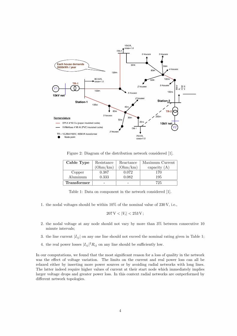
Figure 2: Diagram of the distribution network considered [1].

Cable Type Resistance Reactance Maximum Current(Ohm/km) (Ohm/km) capacity (A)

Copper 0.387 0.072 170Aluminum 0.333 0.082 195

Transformer - - 725

Table 1: Data on component in the network considered [1].

1. the nodal voltages should be within 10% of the nominal value of 230 V, i.e.,

207 V < |Vi| < 253 V ;

2. the nodal voltage at any node should not vary by more than 3% between consecutive 10minute intervals;

3. the line current |Iij | on any one line should not exceed the nominal rating given in Table 1;

4. the real power losses |Iij |2Rij on any line should be sufficiently low.

In our computations, we found that the most significant reason for a loss of quality in the networkwas the effect of voltage variation. The limits on the current and real power loss can all berelaxed either by inserting more power sources or by avoiding radial networks with long lines.The latter indeed require higher values of current at their start node which immediately implieslarger voltage drops and greater power loss. In this context radial networks are outperformed bydifferent network topologies.

4

3 Household Load

In order to solve the power flow problem it is necessary at each load bus, to specify the real powerPi (we took the reactive power drain Qi = 0). We therefore have that

Pi = PSi − PL

i − PEVi

where PSi is the power generated by the solar cells, PL

i is the general household load and PEVi is

the load due to the electrical vehicle charging. Each of these terms has a different form and weconsider each separately.

3.1 Distribution of Household Load over Network

The power drain PLi due to consumer load is a time varying variable, that depends stochastically

upon the customer. A typical household will consume around 400 W on average, with a peakload of around 1 kW. This load varies during the day (and is highest in the early evening) andwe will consider the time variation in the next subsection. Similarly, the power drain varies fromone household to the next, dependent, for example, on the number of people living in each house.Data for annual usage (in kW hours) presented by ENDINET is shown in Figure 3. This figureindicates that over one year the total consumption Pi follows a log-normal distribution so thatlog(Pi) has a mean of 7.904 kWh and a variance of 0.5607 kWh, i.e.,

log(Pi) ∼ N(7.904, 0.5607) .

When simulating the performance of the network the households were each assumed to follow thisdistribution, and the time varying household load scaled accordingly, so that the values of PL

i inthe power equation were each treated as random variables with the distribution as above.

Figure 3: Annual household load distribution accross the network and log-normal fit [1].

3.2 Time Evolution of Single Household Load

Figure 4 gives the electricity consumption of an average household as the percentage of the annualelectricity consumption. The data consist of a winter and summer time series, both of one weeklength and a step size of 15 minutes. Assuming a total annual electricity consumption of 3.5 kWh,

5

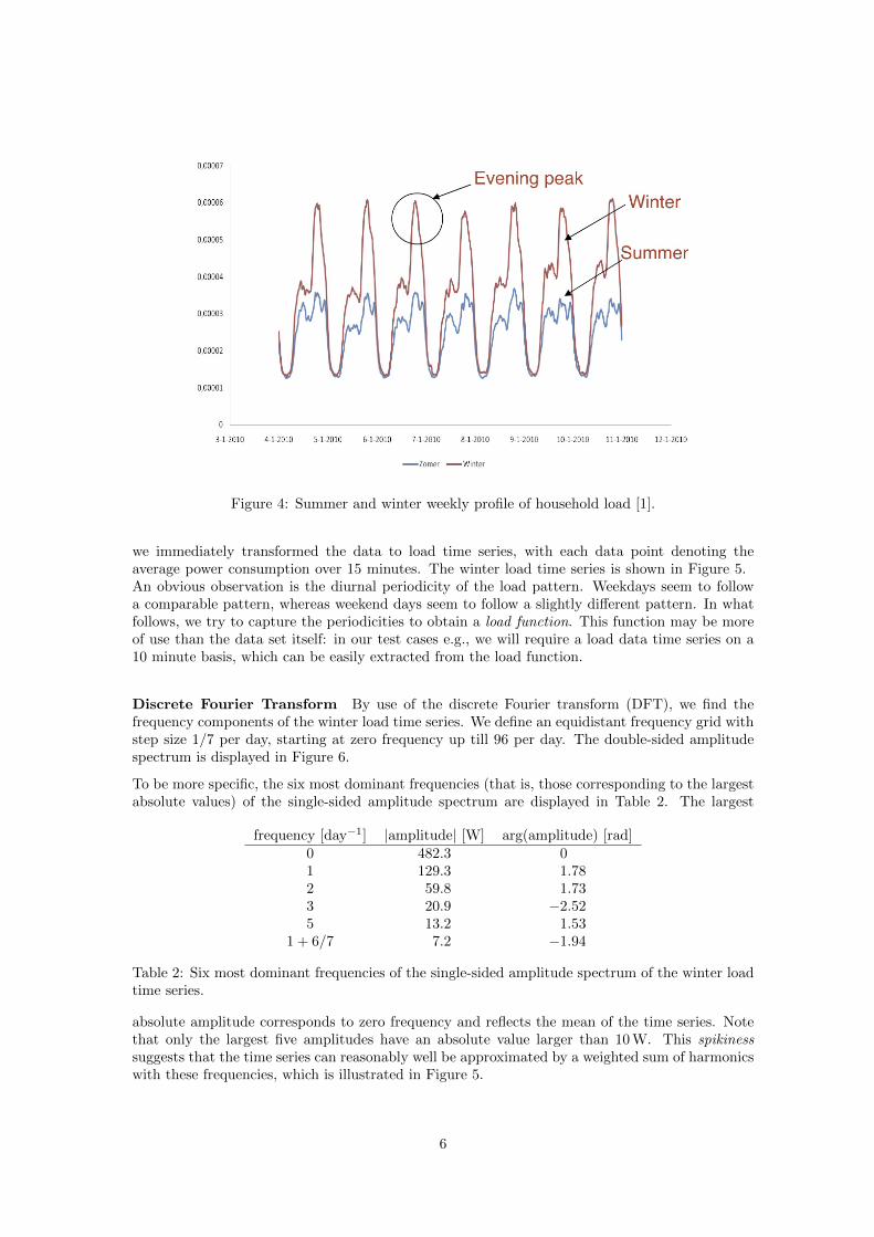
Figure 4: Summer and winter weekly profile of household load [1].

we immediately transformed the data to load time series, with each data point denoting theaverage power consumption over 15 minutes. The winter load time series is shown in Figure 5.An obvious observation is the diurnal periodicity of the load pattern. Weekdays seem to followa comparable pattern, whereas weekend days seem to follow a slightly different pattern. In whatfollows, we try to capture the periodicities to obtain a load function. This function may be moreof use than the data set itself: in our test cases e.g., we will require a load data time series on a10 minute basis, which can be easily extracted from the load function.

Discrete Fourier Transform By use of the discrete Fourier transform (DFT), we find thefrequency components of the winter load time series. We define an equidistant frequency grid withstep size 1/7 per day, starting at zero frequency up till 96 per day. The double-sided amplitudespectrum is displayed in Figure 6.

To be more specific, the six most dominant frequencies (that is, those corresponding to the largestabsolute values) of the single-sided amplitude spectrum are displayed in Table 2. The largest

frequency [day−1] |amplitude| [W] arg(amplitude) [rad]0 482.3 −0.001 129.3 −1.782 059.8 −1.733 020.9 −2.525 013.2 −1.53

1 + 6/7 007.2 −1.94

Table 2: Six most dominant frequencies of the single-sided amplitude spectrum of the winter loadtime series.

absolute amplitude corresponds to zero frequency and reflects the mean of the time series. Notethat only the largest five amplitudes have an absolute value larger than 10 W. This spikinesssuggests that the time series can reasonably well be approximated by a weighted sum of harmonicswith these frequencies, which is illustrated in Figure 5.

6

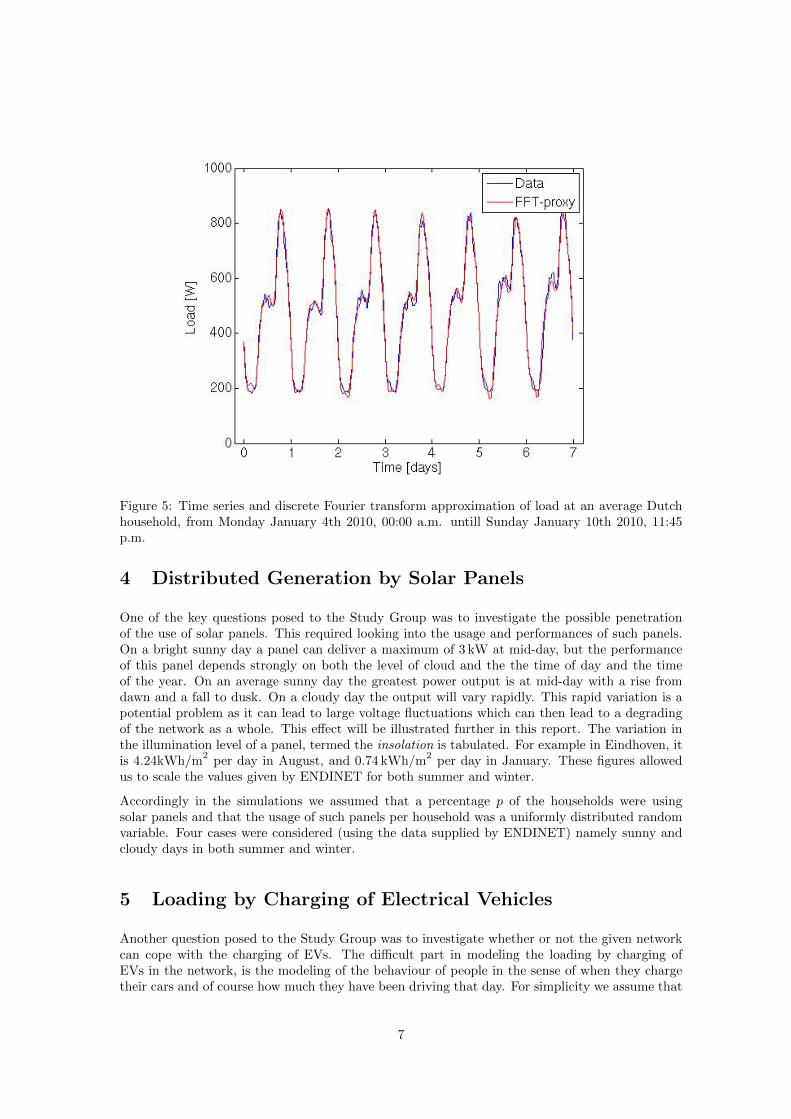
Figure 5: Time series and discrete Fourier transform approximation of load at an average Dutchhousehold, from Monday January 4th 2010, 00:00 a.m. untill Sunday January 10th 2010, 11:45p.m.

4 Distributed Generation by Solar Panels

One of the key questions posed to the Study Group was to investigate the possible penetrationof the use of solar panels. This required looking into the usage and performances of such panels.On a bright sunny day a panel can deliver a maximum of 3 kW at mid-day, but the performanceof this panel depends strongly on both the level of cloud and the the time of day and the timeof the year. On an average sunny day the greatest power output is at mid-day with a rise fromdawn and a fall to dusk. On a cloudy day the output will vary rapidly. This rapid variation is apotential problem as it can lead to large voltage fluctuations which can then lead to a degradingof the network as a whole. This effect will be illustrated further in this report. The variation inthe illumination level of a panel, termed the insolation is tabulated. For example in Eindhoven, itis 4.24kWh/m

2per day in August, and 0.74 kWh/m

2per day in January. These figures allowed

us to scale the values given by ENDINET for both summer and winter.

Accordingly in the simulations we assumed that a percentage p of the households were usingsolar panels and that the usage of such panels per household was a uniformly distributed randomvariable. Four cases were considered (using the data supplied by ENDINET) namely sunny andcloudy days in both summer and winter.

5 Loading by Charging of Electrical Vehicles

Another question posed to the Study Group was to investigate whether or not the given networkcan cope with the charging of EVs. The difficult part in modeling the loading by charging ofEVs in the network, is the modeling of the behaviour of people in the sense of when they chargetheir cars and of course how much they have been driving that day. For simplicity we assume that

7

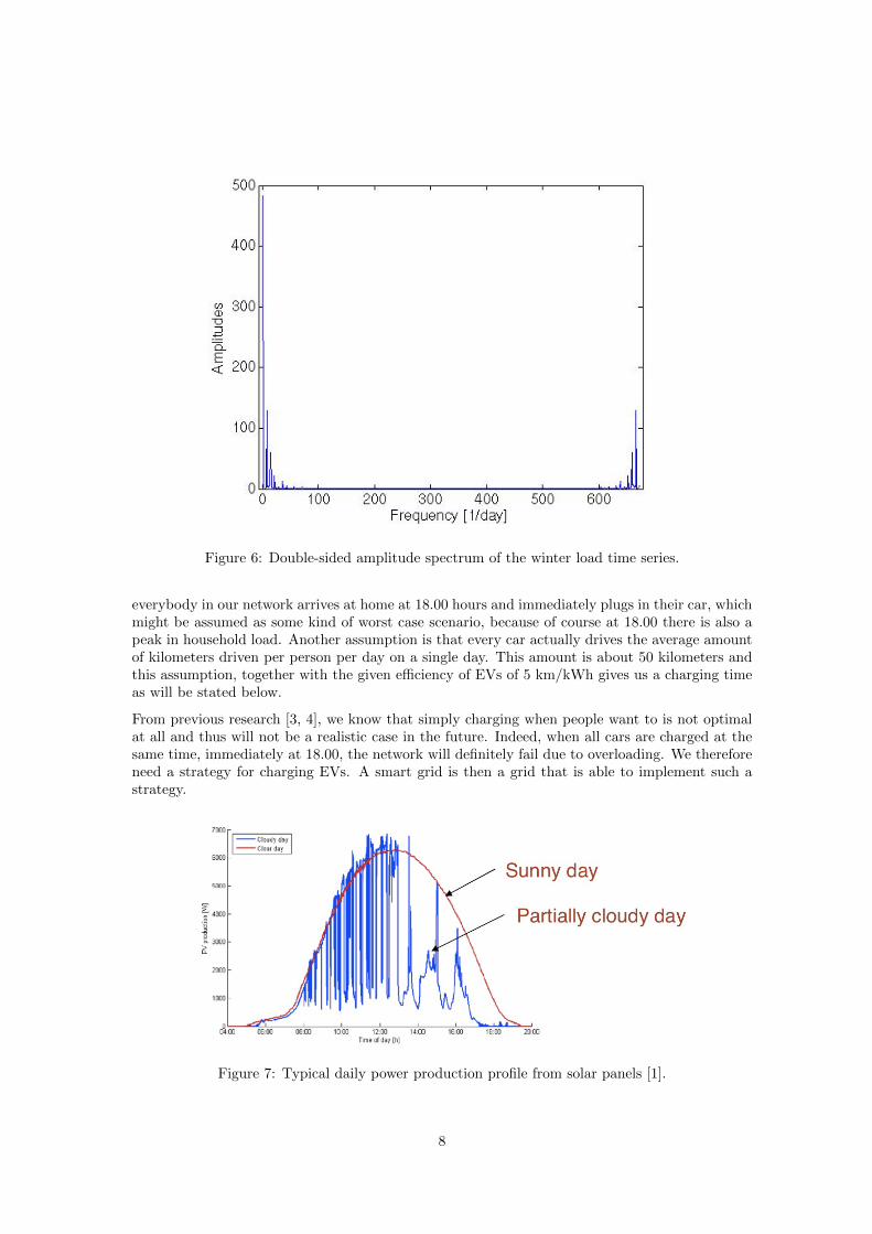
Figure 6: Double-sided amplitude spectrum of the winter load time series.

everybody in our network arrives at home at 18.00 hours and immediately plugs in their car, whichmight be assumed as some kind of worst case scenario, because of course at 18.00 there is also apeak in household load. Another assumption is that every car actually drives the average amountof kilometers driven per person per day on a single day. This amount is about 50 kilometers andthis assumption, together with the given efficiency of EVs of 5 km/kWh gives us a charging timeas will be stated below.

From previous research [3, 4], we know that simply charging when people want to is not optimalat all and thus will not be a realistic case in the future. Indeed, when all cars are charged at thesame time, immediately at 18.00, the network will definitely fail due to overloading. We thereforeneed a strategy for charging EVs. A smart grid is then a grid that is able to implement such astrategy.

Figure 7: Typical daily power production profile from solar panels [1].

8

Of course future work might lead to even better strategies, because we only look at a small pieceof the network might be needed regarding large networks with a lot of EV’s. Our strategy is notoptimal because it does not allow for vehicles charging at loads lower then the maximum one norfor partial charging in case of necessity.

5.1 Greedy Control Strategy for EV Charging

If a customer j arrives at home and wants to charge his car we are given:tj the time at which the customer puts the requestErest

j the energy still left in the carcj the time by which the customer wants the charging to be completed.

Echargedj (optional) the amount of energy that the customer wants to have after

charging. The default value is that the customer wants to have the carcharged fully

Dj the energy requested by the customer, Echargedj − Erest

j

We assume that the customer plugs in his car on the network at time tj . In a smart grid thenetwork can decide when the car is actually charged. The question is now to assign to eachcustomer j an interval that is a subset of [tj ; cj ] during which the the car is charged. This mightbe generalized to a collection of intervals, if we are allowed to preempt the charging of a car. Inthe future, it probably will be possible to charge cars at different speeds.

The problem then becomes a complex scheduling problem. At time tj we have to decide if thecar of customer j is charged or if he has to wait. If we decide to charge the car, we have to makesure that the voltage drop is at most 3 % and that the network constraints on the voltage andcurrent are met during the charging period. Moreover, if there are waiting requests and the powerconsumption in the network decreases, we have to decide whether we start charging another car.Solving this problem requires an intelligent strategy.

In our case study, we restricted ourselves to a basic case. We assume that EV-charging alwaystakes place at 3.5 kW and takes exactly 3 hours requiring therefore 10.5 kWh in total. We alsoassume that charging cannot be preempted. Each household owns one car, which arrives at 18.00and wants to be charged by 07.00 the next morning. We apply the following greedy strategy:

1. Initialization: set time t = 18.00, all customers get state ‘Request’

2. Select from the customers with state ’Request’ the one at the location with largest voltageand check if starting to charge the car of this customer is feasible subject to the networkconstraints.

• If Yes, start charging this car, set state of this customer to ‘Charging’ and updatevoltage and current in the network for the charging time. If there are customers leftwith state ‘Request’ go to Step 2, otherwise we are Finished.

• If No, set t to the next point in time were consumption decreases. If the decrease iscaused by completing the charging of a car, set the state of the customer to ’Complete’Go to Step 2.

An alternative strategy is obtained by selecting a random customer from the set of ‘Request’customers. If charging for this customer is infeasible in the network, we randomly select anothercustomer. We repeat this until we have found a ‘feasible’ customer, or found out that no requestcan be fulfilled. In the latter case, we have to try again at the next point in time where energyconsumption has been decreased. It is not hard to see that this approximates the situation wherecharging requests arrive in a random order.

9

6 Numerical Results

In this section we present numerical results illustrating the impact of distributed generation bysolar panels and loading by the charging of electrical vehicles.

6.1 Distributed Generation by Solar Panels

Impact on Single Node Voltage Figure 8 shows the simulated evolution in time of the voltageof the node with four neighbours in the lower branch of the network for seven consecutive days. Inthis simulation, the power usage of all houses in the network was chosen to be the average powerusage on a typical summer day. The bottom smooth line represents the voltage at the chosen nodewhen no solar panels are present. The voltage at this node is significantly lower than the nominalvalue of 230 V, but still larger than the minimum required voltage of 207 V. The top oscillatoryline represents the voltage at the same node when all houses have solar panels. The solar panelsincrease the voltage in the node up to 7 V, which is only a good thing, as the voltage was alreadyquite low. The graph also shows steep jumps in the voltage. This could cause violation of voltageprofile constraints. Figure 8 does not significantly change if one replaces the assumption of allhouse consuming an average load by a load according to a log-normal distribution.

Impact on Overall Network Performance For every combination of household loads andsolar panel placement four characteristic days are simulated: a cloudy and a sunny day in bothsummer and winter. The network must satisfy all the requirements mentioned in Subsection 2.2in all four conditions to be considered a success. We separately perform the experiment on theoriginal network and on the network with the extra cable.

The scatter plot in Figure 9 displays the results of our Monte Carlo simulations. The solar panelpenetration is plotted along the abscissa and the average household power demand is plottedagainst the ordinate. Both quantities disregard any information about the distribution within thenetwork.

The household power demand has little influence on the network performance. On the other hand,solar panel penetration has a great impact on the network. For penetration levels below 70% thenetwork is robust for any distribution of solar panels and household demand. Above 90% thenetwork fails regardless of distribution, almost exclusively due to excessive jumps in the voltagelevel. For intermediate values the internal distribution of solar panels and household demandhas an influence. But even then the average household usage is of little influence on networkperformance.

We studied the influence of adding a cable (the dotted line in Figure 2) to network performanceby comparing the power loss in the original network to that in the network with the extra cableadded. The household power usage and solar panel distribution were taken randomly in identicalfashion to before, taking an average over the four typical conditions. However only the middayconditions are considered, saving considerable computational time.

The results are presented in Figure 10. It is immediately obvious the extra cable is beneficial tonetwork performance. The power loss over the entire network is approximately halved, regardlessof solar penetration.

The only influence of solar penetration on the network losses is that for intermediate values there ismore variation in the distribution of solar panels throughout the neighbourhood and consequentlythere is some variation in the network losses. But this holds for both network configurationsequally.

10

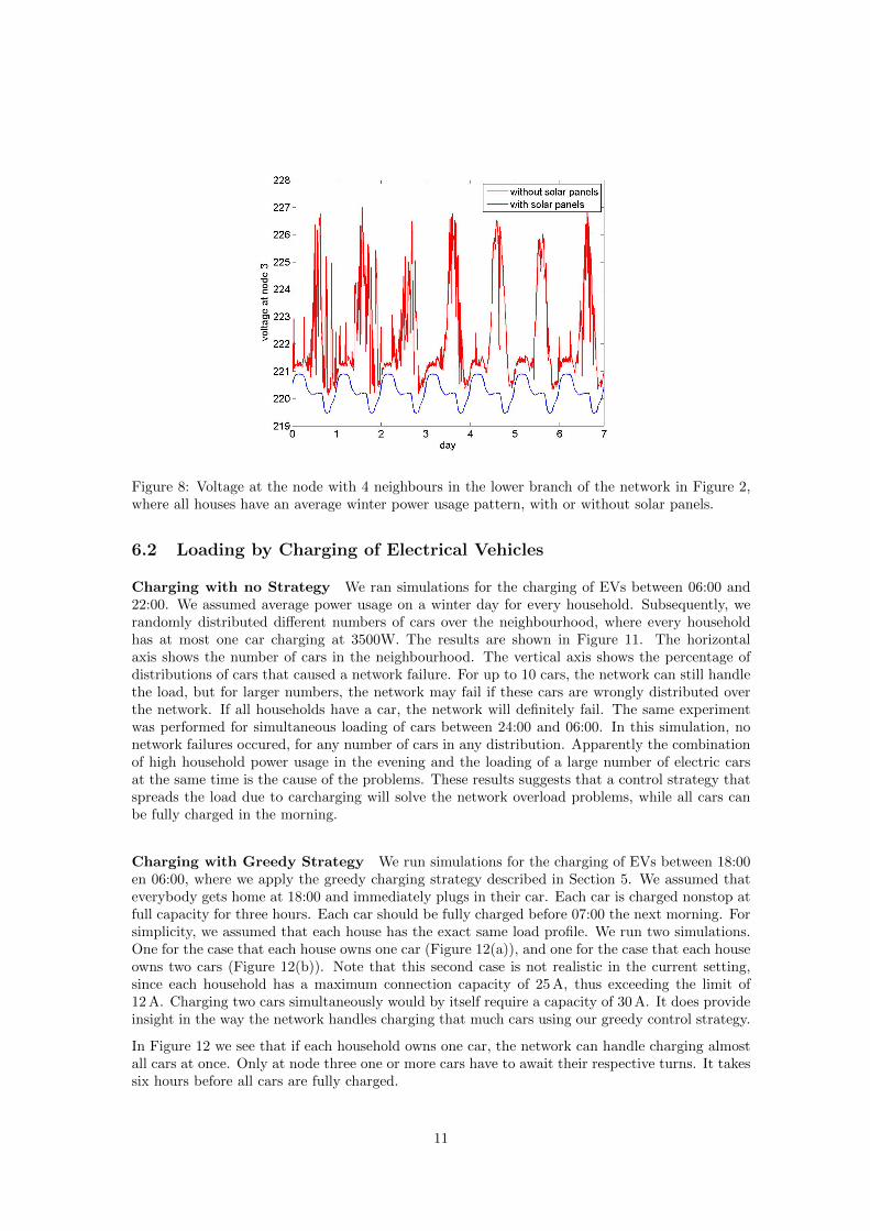
Figure 8: Voltage at the node with 4 neighbours in the lower branch of the network in Figure 2,where all houses have an average winter power usage pattern, with or without solar panels.

6.2 Loading by Charging of Electrical Vehicles

Charging with no Strategy We ran simulations for the charging of EVs between 06:00 and22:00. We assumed average power usage on a winter day for every household. Subsequently, werandomly distributed different numbers of cars over the neighbourhood, where every householdhas at most one car charging at 3500W. The results are shown in Figure 11. The horizontalaxis shows the number of cars in the neighbourhood. The vertical axis shows the percentage ofdistributions of cars that caused a network failure. For up to 10 cars, the network can still handlethe load, but for larger numbers, the network may fail if these cars are wrongly distributed overthe network. If all households have a car, the network will definitely fail. The same experimentwas performed for simultaneous loading of cars between 24:00 and 06:00. In this simulation, nonetwork failures occured, for any number of cars in any distribution. Apparently the combinationof high household power usage in the evening and the loading of a large number of electric carsat the same time is the cause of the problems. These results suggests that a control strategy thatspreads the load due to carcharging will solve the network overload problems, while all cars canbe fully charged in the morning.

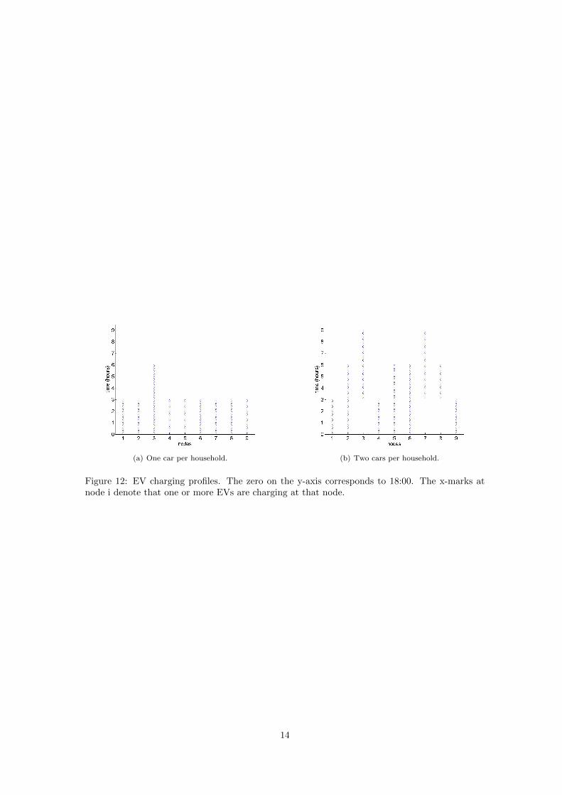
Charging with Greedy Strategy We run simulations for the charging of EVs between 18:00en 06:00, where we apply the greedy charging strategy described in Section 5. We assumed thateverybody gets home at 18:00 and immediately plugs in their car. Each car is charged nonstop atfull capacity for three hours. Each car should be fully charged before 07:00 the next morning. Forsimplicity, we assumed that each house has the exact same load profile. We run two simulations.One for the case that each house owns one car (Figure 12(a)), and one for the case that each houseowns two cars (Figure 12(b)). Note that this second case is not realistic in the current setting,since each household has a maximum connection capacity of 25 A, thus exceeding the limit of12 A. Charging two cars simultaneously would by itself require a capacity of 30 A. It does provideinsight in the way the network handles charging that much cars using our greedy control strategy.

In Figure 12 we see that if each household owns one car, the network can handle charging almostall cars at once. Only at node three one or more cars have to await their respective turns. It takessix hours before all cars are fully charged.

11

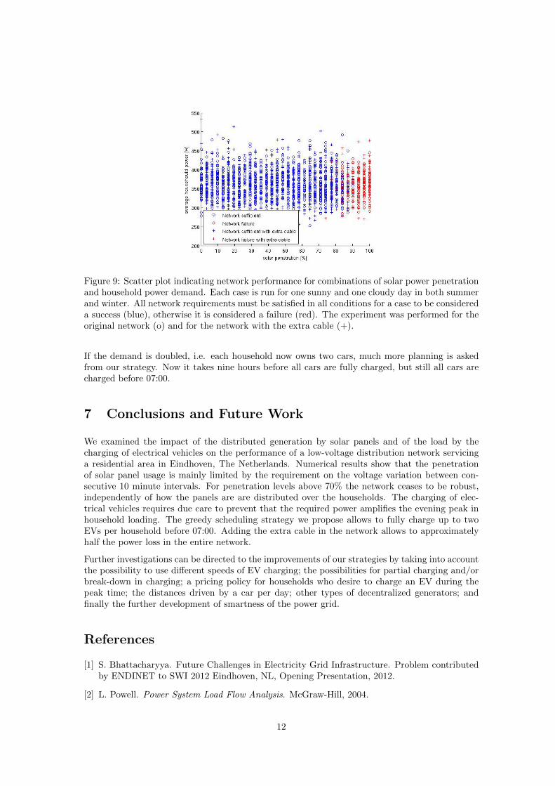
Figure 9: Scatter plot indicating network performance for combinations of solar power penetrationand household power demand. Each case is run for one sunny and one cloudy day in both summerand winter. All network requirements must be satisfied in all conditions for a case to be considereda success (blue), otherwise it is considered a failure (red). The experiment was performed for theoriginal network (o) and for the network with the extra cable (+).

If the demand is doubled, i.e. each household now owns two cars, much more planning is askedfrom our strategy. Now it takes nine hours before all cars are fully charged, but still all cars arecharged before 07:00.

7 Conclusions and Future Work

We examined the impact of the distributed generation by solar panels and of the load by thecharging of electrical vehicles on the performance of a low-voltage distribution network servicinga residential area in Eindhoven, The Netherlands. Numerical results show that the penetrationof solar panel usage is mainly limited by the requirement on the voltage variation between con-secutive 10 minute intervals. For penetration levels above 70% the network ceases to be robust,independently of how the panels are are distributed over the households. The charging of elec-trical vehicles requires due care to prevent that the required power amplifies the evening peak inhousehold loading. The greedy scheduling strategy we propose allows to fully charge up to twoEVs per household before 07:00. Adding the extra cable in the network allows to approximatelyhalf the power loss in the entire network.

Further investigations can be directed to the improvements of our strategies by taking into accountthe possibility to use different speeds of EV charging; the possibilities for partial charging and/orbreak-down in charging; a pricing policy for households who desire to charge an EV during thepeak time; the distances driven by a car per day; other types of decentralized generators; andfinally the further development of smartness of the power grid.

References

[1] S. Bhattacharyya. Future Challenges in Electricity Grid Infrastructure. Problem contributedby ENDINET to SWI 2012 Eindhoven, NL, Opening Presentation, 2012.

[2] L. Powell. Power System Load Flow Analysis. McGraw-Hill, 2004.

12

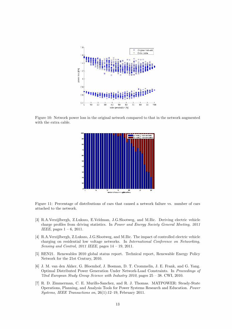
Figure 10: Network power loss in the original network compared to that in the network augmentedwith the extra cable.

Figure 11: Percentage of distributions of cars that caused a network failure vs. number of carsattached to the network.

[3] R.A.Verzijlbergh, Z.Lukszo, E.Veldman, J.G.Slootweg, and M.Ilic. Deriving electric vehiclecharge profiles from driving statistics. In Power and Energy Society General Meeting, 2011IEEE, pages 1 – 6, 2011.

[4] R.A.Verzijlbergh, Z.Lukszo, J.G.Slootweg, and M.Ilic. The impact of controlled electric vehiclecharging on residential low voltage networks. In International Conference on Networking,Sensing and Control, 2011 IEEE, pages 14 – 19, 2011.

[5] REN21. Renewables 2010 global status report. Technical report, Renewable Energy PolicyNetwork for the 21st Century, 2010.

[6] J. M. van den Akker, G. Bloemhof, J. Bosman, D. T. Crommelin, J. E. Frank, and G. Yang.Optimal Distributed Power Generation Under Network-Load Constraints. In Proceedings of72nd European Study Group Science with Industry 2010, pages 25 – 38. CWI, 2010.

[7] R. D. Zimmerman, C. E. Murillo-Sanchez, and R. J. Thomas. MATPOWER: Steady-StateOperations, Planning, and Analysis Tools for Power Systems Research and Education. PowerSystems, IEEE Transactions on, 26(1):12–19, February 2011.

13

(a) One car per household. (b) Two cars per household.

Figure 12: EV charging profiles. The zero on the y-axis corresponds to 18:00. The x-marks atnode i denote that one or more EVs are charging at that node.

14