Embed Size (px)
Citation preview
Délia Canha Gouveia ReisDOCTORATE IN MATHEMATICSSPECIALTY: PROBABILITY AND STATISTICS
Statistical Modelling ofExtreme Rainfall in Madeira IslandDOCTORAL THESIS
SUPERVISORSLuiz Carlos Guerreiro Lopes
Sandra Maria Freitas Mendonça


Statistical Modelling of Extreme Rainfall inMadeira Island
Thesis presented by
Delia Canha Gouveia Reis
and unanimously approved on 12 December 2014,
in public session to obtain the PhD Degree in Mathematics
Jury
Chairman:
Doctor Maria Teresa Alves Homem de Gouveia
(by delegation of authority of the Rector of the Universidade da Madeira)
Members of the Committee (in alphabetical order):
Doctor Dinis Duarte Ferreira Pestana
Full Professor, Universidade de Lisboa
Doctor Joao Alexandre Medina Corte-Real
Full Professor, Universidade de Evora
Doctor Luiz Carlos Guerreiro Lopes
Assistant Professor, Universidade da Madeira
Doctor Rita Cabral Pereira de Castro Guimaraes
Assistant Professor, Universidade de Evora
Doctor Sandra Maria Freitas Mendonca
Assistant Professor, Universidade da Madeira
Doctor Sılvio Filipe Velosa
Assistant Professor, Universidade da Madeira


Abstract
Statistical Modelling of Extreme Rainfall in Madeira Island
Extreme rainfall events have triggered a significant number of flash floods in
Madeira Island along its past and recent history. Madeira is a volcanic island where
the spatial rainfall distribution is strongly affected by its rugged topography. In this
thesis, annual maximum of daily rainfall data from 25 rain gauge stations located in
Madeira Island were modelled by the generalised extreme value distribution. Also,
the hypothesis of a Gumbel distribution was tested by two methods and the existence
of a linear trend in both distributions parameters was analysed. Estimates for the
50– and 100–year return levels were also obtained. Still in an univariate context,
the assumption that a distribution function belongs to the domain of attraction
of an extreme value distribution for monthly maximum rainfall data was tested
for the rainy season. The available data was then analysed in order to find the
most suitable domain of attraction for the sampled distribution. In a different
approach, a search for thresholds was also performed for daily rainfall values through
a graphical analysis. In a multivariate context, a study was made on the dependence
between extreme rainfall values from the considered stations based on Kendall’s
τ measure. This study suggests the influence of factors such as altitude, slope
orientation, distance between stations and their proximity of the sea on the spatial
distribution of extreme rainfall. Groups of three pairwise associated stations were
also obtained and an adjustment was made to a family of extreme value copulas
involving the Marshall–Olkin family, whose parameters can be written as a function
of Kendall’s τ association measures of the obtained pairs.
Keywords: statistics of extremes, annual maxima method, extreme domain of
attraction, threshold choice, copula functions, extreme rainfall.
v

Resumo
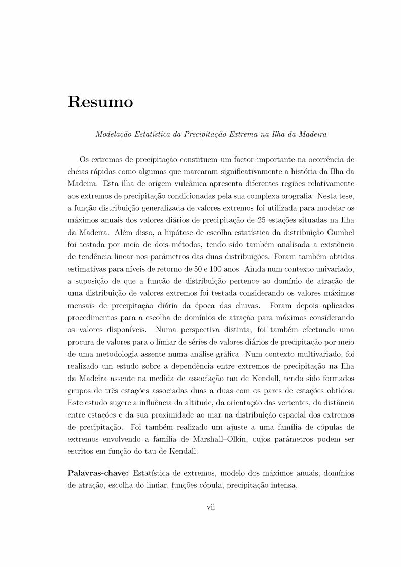
Modelacao Estatıstica da Precipitacao Extrema na Ilha da Madeira
Os extremos de precipitacao constituem um factor importante na ocorrencia de
cheias rapidas como algumas que marcaram significativamente a historia da Ilha da
Madeira. Esta ilha de origem vulcanica apresenta diferentes regioes relativamente
aos extremos de precipitacao condicionadas pela sua complexa orografia. Nesta tese,
a funcao distribuicao generalizada de valores extremos foi utilizada para modelar os
maximos anuais dos valores diarios de precipitacao de 25 estacoes situadas na Ilha
da Madeira. Alem disso, a hipotese de escolha estatıstica da distribuicao Gumbel
foi testada por meio de dois metodos, tendo sido tambem analisada a existencia
de tendencia linear nos parametros das duas distribuicoes. Foram tambem obtidas
estimativas para nıveis de retorno de 50 e 100 anos. Ainda num contexto univariado,
a suposicao de que a funcao de distribuicao pertence ao domınio de atracao de
uma distribuicao de valores extremos foi testada considerando os valores maximos
mensais de precipitacao diaria da epoca das chuvas. Foram depois aplicados
procedimentos para a escolha de domınios de atracao para maximos considerando
os valores disponıveis. Numa perspectiva distinta, foi tambem efectuada uma
procura de valores para o limiar de series de valores diarios de precipitacao por meio
de uma metodologia assente numa analise grafica. Num contexto multivariado, foi
realizado um estudo sobre a dependencia entre extremos de precipitacao na Ilha
da Madeira assente na medida de associacao tau de Kendall, tendo sido formados
grupos de tres estacoes associadas duas a duas com os pares de estacoes obtidos.
Este estudo sugere a influencia da altitude, da orientacao das vertentes, da distancia
entre estacoes e da sua proximidade ao mar na distribuicao espacial dos extremos
de precipitacao. Foi tambem realizado um ajuste a uma famılia de copulas de
extremos envolvendo a famılia de Marshall–Olkin, cujos parametros podem ser
escritos em funcao do tau de Kendall.
Palavras-chave: Estatıstica de extremos, modelo dos maximos anuais, domınios
de atracao, escolha do limiar, funcoes copula, precipitacao intensa.
vii


Acknowledgements
To Professors Luiz Lopes and Sandra Mendonca, my supervisors, for encouraging
me to work in the area of extreme value analysis and for suggesting the topic of the
present thesis. The generosity with which they offered their time and ideas to
this work is also appreciated. I would also like to acknowledge their support and
encouragement to participate in scientific meetings and their confidence in my work.
To the Portuguese Foundation for Science and Technology (FCT), for
the financial support through the PhD grant SFRH/BD/39226/2007, financed by
national funds of the Ministry of Science, Technology and Higher Education (MCTES).
I am also grateful to the Centre of Statistics and Applications of the University
of Lisbon (CEAUL) for the bibliographical and financial support through FCT
projects PEst-OE/MAT/UI0006/2011 and PEst-OE/MAT/UI0006/2014. To the
University of Madeira for providing the appropriate conditions for the realisation of
this thesis and for the logistic support.
To the Portuguese Institute for Sea and Atmosphere (IPMA), namely to Doctor
Victor Prior, for providing the monthly maximum rainfall data used in this thesis.
Thanks are also due to the Department of Hydraulics and Energy Technologies
of the Madeira Regional Laboratory of Civil Engineering (LREC), in particular to
Doctor Carlos Magro, for making available the daily rainfall data from 25 rain gauge
stations maintained in the past by the General Council of the Autonomous District
of Funchal.
I would also like to express my gratitude and appreciation to all those I have
had the opportunity and the pleasure to learn and work with directly in courses of
Statistics and Probability: Professor Ana Abreu, Professor Paulo Freitas, Professor
Rita Vasconcelos, Professor Sandra Mendonca and Professor Sılvio Velosa. A special
acknowledgement to Professor Rita Vasconcelos for her guidance when I first needed
to use a statistical software, for all the concise and fruitful meetings about the courses
I taught as her assistant, and for all the encouragement throughout the elaboration of
ix

x
this thesis. I would also like to thank Professors Rita Vasconcelos and Paulo Freitas
for sparing me from the grading task in the last weeks of the second semester of the
academic year 2013/2014, so that I could dedicate some more time to the conclusion
of the writing of this thesis. I am also grateful to Professors Ana Abreu and Sılvio
Velosa for all their efforts to offer me precious time to dedicate to the elaboration of
this thesis throughout the later five years. A special acknowledgement to Professor
Ana Abreu for introducing me the R software and language, which was essential for
the work developed and described here. I would also like to thank Professor Ana
Abreu for the classes about the R software functionalities and also for the tips about
R packages concerning maps, which were used in this thesis.
To all other colleagues at the Centre for Exact Sciences and Engineering for all
their contributions to my education as a student and as a teacher. I am also grateful
for their friendship and their support. A special acknowledgement to Professor
Custodia Drumond for the encouragement, the care and also for the tea breaks
which brightened many afternoons. A special acknowledgement to Professor Jose
Carmo for having always assured me the best possible working conditions and for
the constant encouragement throughout the elaboration of this thesis.
I would also like to express my appreciation to the participants of the scientific
meetings organised by the Portuguese Society of Statistics (SPE) from whom I had
the opportunity to learn. In particular, I would like to thank Professor Ivette Gomes
for the encouraging comments and guidance about a work I presented in one of those
meetings. A special acknowledgement to Professor Dinis Pestana for the guidance
and bibliographical support.
To all my (present and former) students for the motivation that comes from the
pleasure of lecturing to them.
To Maurıcio’s family (now also mine) for receiving me with open arms and also
for their friendship, support and care.
To Analuce, my sister, for personifying the persistence in the pursuit of aims and
dreams. To Lucia and Antonio, my parents, for personifying the strength and joy
of living. Thanks for all the support, care and love. I am blessed to have you three
in my life.
To Maurıcio, for listening, cheering and caring.
Contents
List of Acronyms and Symbols xiii
List of Figures xv
List of Tables xxiii
1 Introduction 1
1.1 Aims and contributions . . . . . . . . . . . . . . . . . . . . . . . . . . 2
1.2 Organization of the thesis . . . . . . . . . . . . . . . . . . . . . . . . 5
2 State of the art (and a taste of the history of extreme value theory) 7
2.1 Univariate and multivariate extreme value approaches . . . . . . . . . 10
2.2 Application to rainfall extremes . . . . . . . . . . . . . . . . . . . . . 13
3 About Madeira Island’s climate characteristics, flash flood history
and rainfall data 17
4 Methodology 29
4.1 Gumbel’s model approach . . . . . . . . . . . . . . . . . . . . . . . . 29
4.1.1 Extreme value distributions . . . . . . . . . . . . . . . . . . . 30
4.1.2 Parameter estimation methods and statistical tests . . . . . . 32
4.1.3 Plots and statistical tests for model diagnostics . . . . . . . . 37
4.1.4 A trend analysis . . . . . . . . . . . . . . . . . . . . . . . . . . 39
4.2 About extreme domains of attraction, number of observations above
a random threshold and threshold choices . . . . . . . . . . . . . . . . 41
4.3 An extreme value copula approach . . . . . . . . . . . . . . . . . . . 46
5 Results and discussion 57
5.1 Annual maxima – Gumbel’s model approach . . . . . . . . . . . . . . 57
5.1.1 Dataset I . . . . . . . . . . . . . . . . . . . . . . . . . . . . . 58
5.1.2 Dataset II . . . . . . . . . . . . . . . . . . . . . . . . . . . . . 67
xi

xii CONTENTS
5.1.3 Dataset I+II . . . . . . . . . . . . . . . . . . . . . . . . . . . . 81
5.2 Monthly and daily precipitation data – PORT and POT approaches . 89
5.2.1 Statistical choice of extreme domains of attraction . . . . . . . 90
5.2.2 Threshold choice in a POT approach . . . . . . . . . . . . . . 97
5.3 Spatial annual maxima – Copula functions . . . . . . . . . . . . . . . 104
5.3.1 Dataset V . . . . . . . . . . . . . . . . . . . . . . . . . . . . . 106
5.3.2 Dataset VI . . . . . . . . . . . . . . . . . . . . . . . . . . . . . 112
5.3.3 Dataset VII . . . . . . . . . . . . . . . . . . . . . . . . . . . . 121
6 Conclusion 129
References 137
Appendix 157
A Diagnostic plots for annual maxima – Dataset I 159
B Likelihood ratio tests’s p–values – Datasets II and I+II 167
C Diagnostic plots for annual maxima – Dataset II (Class 1) 171
D Diagnostic plots for annual maxima – Dataset II (Class 2) 177
E Diagnostic plots for annual maxima – Dataset II (Class 3) 185
F Diagnostic plots for annual maxima – Dataset II (Class 4) 193
G Diagnostic plots for annual maxima – Dataset I+II 203
H Threshold choice plots – Dataset IV (Class 1) 209
I Threshold choice plots – Dataset IV (Class 2) 213
J Threshold choice plots – Dataset IV (Class 3) 221
K Threshold choice plots – Dataset IV (Class 4) 227
L Exceedances percentage by month – Dataset IV 235
M Code of the functions implemented in R 239
List of Acronyms and Symbols
ASI Advanced Statistical Institute
EVC extreme value copula
GEV generalised extreme value
GPD generalised Pareto distribution
IPMA Portuguese Institute for the Sea and Atmosphere
LREC Regional Laboratory of Civil Engineering
ML maximum likelihood
POT peaks over threshold
PORT peaks over random threshold
PWM probability weighted moments
d−→ converges in distribution to
dX,Y distance in meters between stations X and Y
qp 1/p–year return level estimate
qMα 1/α–year return level estimate calculated by the method M (α ∈ (0, 1))
χ2k chi–square distribution with k degrees of freedom
rα return period of Eα = P (Xi > xi,α) for i ∈ {1, 2, 3} and α ∈ (0, 1)
Xi observation at the i–th rain gauge station
xi,q (1− q)–quantile of Xi for q ∈ (0, 1) and i ∈ {1, 2, 3}x1:n, ..., xn:n ascending order statistics of the sample (x1, . . . , xn)
x(1), ..., x(k) exceedances
τX,Yn estimates based on a sample of size n of Kendall’s τ association
measure between stations X and Y
xiii

List of Figures
3.1 Location and altitude range of the rain gauge stations–Set LREC
(Map data c©2014 Google). . . . . . . . . . . . . . . . . . . . . . . . 20
3.2 Annual maximum of daily precipitation values at Areeiro (A) (up
left), Bica da Cana (B) (up right), Santo da Serra (I) (down left),
and Santana (P) (down right) stations–Set IPMA. . . . . . . . . . . . 25
3.3 Annual maximum of daily precipitation values at Funchal (U) (up
left), Santa Catarina (V) (up right), and Lugar de Baixo (X) (down)
stations–Set IPMA. . . . . . . . . . . . . . . . . . . . . . . . . . . . . 26
3.4 Annual maximum of daily precipitation values at Poiso (C) (up left),
Montado do Pereiro (D) (up right), Encumeada (E) (down left), and
Ribeiro Frio (F) (down right) stations–Set LREC. . . . . . . . . . . . 26
3.5 Annual maximum of daily precipitation values at Queimadas (G)
(up left), Camacha (H) (up right), and Porto Moniz (J) (down)
stations–Set LREC. . . . . . . . . . . . . . . . . . . . . . . . . . . . . 27
3.6 Annual maximum of daily precipitation values at Curral das
Freiras (K) (up left), Ponta do Pargo (L) (up right), Santo
Antonio (M) (down left), and Canhas (N) (down right) stations–
Set LREC. . . . . . . . . . . . . . . . . . . . . . . . . . . . . . . . . . 27
3.7 Annual maximum of daily precipitation values at Sanatorio (O)
(up left), Loural (Q) (up right), and Bom Sucesso (R) (down)
stations–Set LREC. . . . . . . . . . . . . . . . . . . . . . . . . . . . . 28
3.8 Annual maximum of daily precipitation values at Machico (S)
(up left), Ponta Delgada (T) (up right), Canical (W) (down left),
and Ribeira Brava (Y) (down right) stations–Set LREC. . . . . . . . 28
5.1 Location and altitude range of the rain gauge stations–Dataset I (Map
data c©2014 Google). . . . . . . . . . . . . . . . . . . . . . . . . . . . . 58
xv
xvi LIST OF FIGURES
5.2 Profile log-likelihood for γ in Model 1 for Areeiro (A) (up left), Bica
da Cana (B) (up right), Santo da Serra (I) (down left), and Santana
(P) (down right) stations. . . . . . . . . . . . . . . . . . . . . . . . . 61
5.3 Profile log-likelihood for γ in Model 1 for Funchal (U) (up left), Santa
Catarina (V) (up right) and Lugar de Baixo (X) (down) stations. . . 62
5.4 Diagnostic plots for non-Gumbel GEV fit to the Funchal (U) station
data–Dataset I. . . . . . . . . . . . . . . . . . . . . . . . . . . . . . . 65
5.5 Diagnostic plots for Gumbel fit to the Funchal (U) station data–
Dataset I. . . . . . . . . . . . . . . . . . . . . . . . . . . . . . . . . . 65
5.6 Location and altitude range of the rain gauge stations–Dataset II
(Map data c©2014 Google). . . . . . . . . . . . . . . . . . . . . . . . . 68
5.7 Annual maximum of daily precipitation values at Areeiro (A) (up
left), Bica da Cana (B) (up right), Santo da Serra (I) (down left),
and Santana (P) (down right) stations–Dataset II. . . . . . . . . . . . 71
5.8 Annual maximum of daily precipitation values at Funchal (U) (up
left), Santa Catarina (V) (up right), and Lugar de Baixo (X) (down)
stations–Dataset II. . . . . . . . . . . . . . . . . . . . . . . . . . . . . 72
5.9 Diagnostic plots for GEV fit to the Ribeira Brava (Y) station data–
Dataset II. . . . . . . . . . . . . . . . . . . . . . . . . . . . . . . . . . 78
5.10 Diagnostic plots for GEV fit to the Ponta Delgada (T) station data–
Dataset II. . . . . . . . . . . . . . . . . . . . . . . . . . . . . . . . . . 78
5.11 Annual maximum daily precipitation values at Areeiro (A) (up left),
Bica da Cana (B) (up right), Santo da Serra (I) (down left), and
Lugar de Baixo (X) (down right) stations–Dataset I+II. . . . . . . . . 83
5.12 Diagnostic plots for GEV distribution fit to the Santo da Serra (I)
station data–Dataset I+II. . . . . . . . . . . . . . . . . . . . . . . . . 87
5.13 Diagnostic plots for GEV ditribution fit to the Santa Catarina (V)
station data–Dataset I+II. . . . . . . . . . . . . . . . . . . . . . . . . 87
5.14 Location and altitude range of the rain gauge stations–Dataset III
(Map data c©2014 Google). . . . . . . . . . . . . . . . . . . . . . . . . 90
5.15 Values of the test statistic En(k) (solid) and the 0.95 quantile (dotted)
applied to the datasets from Areeiro (A) (up left), Santo da Serra (I)
(up right) and Santana (P) (down) stations. . . . . . . . . . . . . . . 92
5.16 Values of the test statistic En(k) (solid) and the 0.95 quantile (dotted)
applied to the datasets from Bica da Cana (B) (up left), Funchal (U)
(up right), Santa Catarina (V) (down left) and Lugar de Baixo (X)
(down right) stations. . . . . . . . . . . . . . . . . . . . . . . . . . . . 93
LIST OF FIGURES xvii
5.17 Values of the test statistics W ∗n (solid) and R∗n (dotted) applied to the
datasets from Areeiro (A) (up left), Bica da Cana (B) (up right) and
Santo da Serra (I) (down) stations. . . . . . . . . . . . . . . . . . . . 95
5.18 Values of the test statistics W ∗n (solid) and R∗n (dotted) applied to the
datasets from Santana (P) (up left), Funchal (U) (up right), Santa
Catarina (V) (down left) and Lugar de Baixo (X) (down right) stations. 96
5.19 Location and altitude range of the rain gauge stations–Dataset IV
(Map data c©2014 Google). . . . . . . . . . . . . . . . . . . . . . . . . 97
5.20 Mean residual plot for the Areeiro (A) (up left), Encumeada (E) (up
right), Canhas (N) (down left) and Funchal (U) (down right) stations
data. . . . . . . . . . . . . . . . . . . . . . . . . . . . . . . . . . . . . 98
5.21 Parameter stability plots for the Areeiro (A) station data. . . . . . . 99
5.22 Parameter stability plots for the Encumeada (E) station data. . . . . 99
5.23 Parameter stability plots for the Canhas (N) station data. . . . . . . 100
5.24 Parameter stability plots for the Funchal (U) station data. . . . . . . 100
5.25 Location and altitude range of the rain gauge stations–Dataset V
(Map data c©2014 Google). . . . . . . . . . . . . . . . . . . . . . . . . 106
5.26 Location and altitude range of the rain gauge stations–Dataset VI
(Map data c©2014 Google). . . . . . . . . . . . . . . . . . . . . . . . . 112
5.27 Location and altitude range of the rain gauge stations–Dataset VI
(Map data c©2014 Google). . . . . . . . . . . . . . . . . . . . . . . . . 122
A.1 Diagnostic plots for Gumbel fit to the Areeiro (A) station data–
Dataset I. . . . . . . . . . . . . . . . . . . . . . . . . . . . . . . . . . 160
A.2 Diagnostic plots for GEV fit to the Areeiro (A) station data–Dataset I.160
A.3 Diagnostic plots for Gumbel fit to the Bica da Cana (B) station data–
Dataset I. . . . . . . . . . . . . . . . . . . . . . . . . . . . . . . . . . 161
A.4 Diagnostic plots for GEV fit to the Bica da Cana (B) station data–
Dataset I. . . . . . . . . . . . . . . . . . . . . . . . . . . . . . . . . . 161
A.5 Diagnostic plots for Gumbel fit to the Santo da Serra (I) station
data–Dataset I. . . . . . . . . . . . . . . . . . . . . . . . . . . . . . . 162
A.6 Diagnostic plots for GEV fit to the Santo da Serra (I) station data–
Dataset I. . . . . . . . . . . . . . . . . . . . . . . . . . . . . . . . . . 162
A.7 Diagnostic plots for Gumbel fit to the Santana (P) station data–
Dataset I. . . . . . . . . . . . . . . . . . . . . . . . . . . . . . . . . . 163
A.8 Diagnostic plots for GEV fit to the Santana (P) station data–Dataset I.163
xviii LIST OF FIGURES
A.9 Diagnostic plots for Gumbel fit to the Santa Catarina (V) station
data–Dataset I. . . . . . . . . . . . . . . . . . . . . . . . . . . . . . . 164
A.10 Diagnostic plots for GEV fit to the Santa Catarina (V) station data–
Dataset I. . . . . . . . . . . . . . . . . . . . . . . . . . . . . . . . . . 164
A.11 Diagnostic plots for Gumbel fit to the Lugar de Baixo (X) station
data–Dataset I. . . . . . . . . . . . . . . . . . . . . . . . . . . . . . . 165
A.12 Diagnostic plots for GEV fit to the Lugar de Baixo (X) station data–
Dataset I. . . . . . . . . . . . . . . . . . . . . . . . . . . . . . . . . . 165
C.1 Diagnostic plots for Gumbel fit to the Areeiro (A) station data–
Dataset II. . . . . . . . . . . . . . . . . . . . . . . . . . . . . . . . . . 172
C.2 Diagnostic plots for GEV fit to the Areeiro (A) station data–Dataset II.172
C.3 Diagnostic plots for Gumbel fit to the Bica da Cana (B) station data–
Dataset II. . . . . . . . . . . . . . . . . . . . . . . . . . . . . . . . . . 173
C.4 Diagnostic plots for GEV fit to the Bica da Cana (B) station data–
Dataset II. . . . . . . . . . . . . . . . . . . . . . . . . . . . . . . . . . 173
C.5 Diagnostic plots for Gumbel fit to the Poiso (C) station data–Dataset II.174
C.6 Diagnostic plots for GEV fit to the Poiso (C) station data–Dataset II. 174
C.7 Diagnostic plots for Gumbel fit to the Montado do Pereiro (D) station
data–Dataset II. . . . . . . . . . . . . . . . . . . . . . . . . . . . . . . 175
C.8 Diagnostic plots for GEV fit to the Montado do Pereiro (D) station
data–Dataset II. . . . . . . . . . . . . . . . . . . . . . . . . . . . . . . 175
D.1 Diagnostic plots for Gumbel fit to the Encumeada (E) station data–
Dataset II. . . . . . . . . . . . . . . . . . . . . . . . . . . . . . . . . . 178
D.2 Diagnostic plots for GEV fit to the Encumeada (E) station data–
Dataset II. . . . . . . . . . . . . . . . . . . . . . . . . . . . . . . . . . 178
D.3 Diagnostic plots for Gumbel fit to the Ribeiro Frio (F) station data–
Dataset II. . . . . . . . . . . . . . . . . . . . . . . . . . . . . . . . . . 179
D.4 Diagnostic plots for GEV fit to the Ribeiro Frio (F) station data–
Dataset II. . . . . . . . . . . . . . . . . . . . . . . . . . . . . . . . . . 179
D.5 Diagnostic plots for Gumbel fit to the Queimadas (G) station data–
Dataset II. . . . . . . . . . . . . . . . . . . . . . . . . . . . . . . . . . 180
D.6 Diagnostic plots for GEV fit to the Queimadas (G) station data–
Dataset II. . . . . . . . . . . . . . . . . . . . . . . . . . . . . . . . . . 180
D.7 Diagnostic plots for Gumbel fit to the Camacha (H) station data–
Dataset II. . . . . . . . . . . . . . . . . . . . . . . . . . . . . . . . . . 181

LIST OF FIGURES xix
D.8 Diagnostic plots for GEV fit to the Camacha (H) station data–
Dataset II. . . . . . . . . . . . . . . . . . . . . . . . . . . . . . . . . . 181
D.9 Diagnostic plots for Gumbel fit to the Santo da Serra (I) station
data–Dataset II. . . . . . . . . . . . . . . . . . . . . . . . . . . . . . . 182
D.10 Diagnostic plots for GEV fit to the Santo da Serra (I) station data–
Dataset II. . . . . . . . . . . . . . . . . . . . . . . . . . . . . . . . . . 182
D.11 Diagnostic plots for Gumbel fit to the Porto Moniz (J) station data–
Dataset II. . . . . . . . . . . . . . . . . . . . . . . . . . . . . . . . . . 183
D.12 Diagnostic plots for GEV fit to the Porto Moniz (J) station data–
Dataset II. . . . . . . . . . . . . . . . . . . . . . . . . . . . . . . . . . 183
D.13 Diagnostic plots for Gumbel fit to the Curral das Freiras (K) station
data–Dataset II. . . . . . . . . . . . . . . . . . . . . . . . . . . . . . . 184
D.14 Diagnostic plots for GEV fit to the Curral das Freiras (K) station
data–Dataset II. . . . . . . . . . . . . . . . . . . . . . . . . . . . . . . 184
E.1 Diagnostic plots for Gumbel fit to the Ponta do Pargo (L) station
data–Dataset II. . . . . . . . . . . . . . . . . . . . . . . . . . . . . . . 186
E.2 Diagnostic plots for GEV fit to the Ponta do Pargo (L) station data–
Dataset II. . . . . . . . . . . . . . . . . . . . . . . . . . . . . . . . . . 186
E.3 Diagnostic plots for Gumbel fit to the Santo Antonio (M) station
data–Dataset II. . . . . . . . . . . . . . . . . . . . . . . . . . . . . . . 187
E.4 Diagnostic plots for GEV fit to the Santo Antonio (M) station data–
Dataset II. . . . . . . . . . . . . . . . . . . . . . . . . . . . . . . . . . 187
E.5 Diagnostic plots for Gumbel fit to the Canhas (N) station data–
Dataset II. . . . . . . . . . . . . . . . . . . . . . . . . . . . . . . . . . 188
E.6 Diagnostic plots for GEV fit to the Canhas (N) station data–Dataset II.188
E.7 Diagnostic plots for Gumbel fit to the Sanatorio (O) station data–
Dataset II. . . . . . . . . . . . . . . . . . . . . . . . . . . . . . . . . . 189
E.8 Diagnostic plots for GEV fit to the Sanatorio (O) station data–
Dataset II. . . . . . . . . . . . . . . . . . . . . . . . . . . . . . . . . . 189
E.9 Diagnostic plots for Gumbel fit to the Santana (P) station data–
Dataset II. . . . . . . . . . . . . . . . . . . . . . . . . . . . . . . . . . 190
E.10 Diagnostic plots for GEV fit to the Santana (P) station data–Dataset II.190
E.11 Diagnostic plots for Gumbel fit to the Loural (Q) station data–
Dataset II. . . . . . . . . . . . . . . . . . . . . . . . . . . . . . . . . . 191
E.12 Diagnostic plots for GEV fit to the Loural (Q) station data–Dataset II.191
xx LIST OF FIGURES
F.1 Diagnostic plots for Gumbel fit to the Bom Sucesso (R) station data–
Dataset II. . . . . . . . . . . . . . . . . . . . . . . . . . . . . . . . . . 194
F.2 Diagnostic plots for GEV fit to the Bom Sucesso (R) station data–
Dataset II. . . . . . . . . . . . . . . . . . . . . . . . . . . . . . . . . . 194
F.3 Diagnostic plots for Gumbel fit to the Machico (S) station data–
Dataset II. . . . . . . . . . . . . . . . . . . . . . . . . . . . . . . . . . 195
F.4 Diagnostic plots for GEV fit to the Machico (S) station data–Dataset II.195
F.5 Diagnostic plots for Gumbel fit to the Ponta Delgada (T) station
data–Dataset II. . . . . . . . . . . . . . . . . . . . . . . . . . . . . . . 196
F.6 Diagnostic plots for GEV fit to the Ponta Delgada (T) station data–
Dataset II. . . . . . . . . . . . . . . . . . . . . . . . . . . . . . . . . . 196
F.7 Diagnostic plots for Gumbel fit to the Funchal (U) station data–
Dataset II. . . . . . . . . . . . . . . . . . . . . . . . . . . . . . . . . . 197
F.8 Diagnostic plots for GEV fit to the Funchal (U) station data–Dataset II.197
F.9 Diagnostic plots for Gumbel fit to the Santa Catarina (V) station
data–Dataset II. . . . . . . . . . . . . . . . . . . . . . . . . . . . . . . 198
F.10 Diagnostic plots for GEV fit to the Santa Catarina (V) station data–
Dataset II. . . . . . . . . . . . . . . . . . . . . . . . . . . . . . . . . . 198
F.11 Diagnostic plots for Gumbel fit to the Canical (W) station data–
Dataset II. . . . . . . . . . . . . . . . . . . . . . . . . . . . . . . . . . 199
F.12 Diagnostic plots for GEV fit to the Canical (W) station data–Dataset II.199
F.13 Diagnostic plots for Gumbel fit to the Lugar de Baixo (X) station
data–Dataset II. . . . . . . . . . . . . . . . . . . . . . . . . . . . . . . 200
F.14 Diagnostic plots for GEV fit to the Lugar de Baixo (X) station data–
Dataset II. . . . . . . . . . . . . . . . . . . . . . . . . . . . . . . . . . 200
F.15 Diagnostic plots for Gumbel fit to the Ribeira Brava (Y) station data–
Dataset II. . . . . . . . . . . . . . . . . . . . . . . . . . . . . . . . . . 201
F.16 Diagnostic plots for GEV fit to the Ribeira Brava (Y) station data–
Dataset II. . . . . . . . . . . . . . . . . . . . . . . . . . . . . . . . . . 201
G.1 Diagnostic plots for Gumbel fit to the Areeiro (A) station data–
Dataset I+II. . . . . . . . . . . . . . . . . . . . . . . . . . . . . . . . 204
G.2 Diagnostic plots for GEV fit to the Areeiro (A) station data–
Dataset I+II. . . . . . . . . . . . . . . . . . . . . . . . . . . . . . . . 204
G.3 Diagnostic plots for Gumbel fit to the Bica da Cana (B) station data–
Dataset I+II. . . . . . . . . . . . . . . . . . . . . . . . . . . . . . . . 205
LIST OF FIGURES xxi
G.4 Diagnostic plots for GEV fit to the Bica da Cana (B) station data–
Dataset I+II. . . . . . . . . . . . . . . . . . . . . . . . . . . . . . . . 205
G.5 Diagnostic plots for Gumbel fit to the Santo da Serra (I) station
data–Dataset I+II. . . . . . . . . . . . . . . . . . . . . . . . . . . . . 206
G.6 Diagnostic plots for GEV fit to the Santo da Serra (I) station data–
Dataset I+II. . . . . . . . . . . . . . . . . . . . . . . . . . . . . . . . 206
G.7 Diagnostic plots for Gumbel fit to the Santa Catarina (V) station
data–Dataset I+II. . . . . . . . . . . . . . . . . . . . . . . . . . . . . 207
G.8 Diagnostic plots for GEV fit to the Santa Catarina (V) station data–
Dataset I+II. . . . . . . . . . . . . . . . . . . . . . . . . . . . . . . . 207
G.9 Diagnostic plots for Gumbel fit to the Lugar de Baixo (X) station
data–Dataset I+II. . . . . . . . . . . . . . . . . . . . . . . . . . . . . 208
G.10 Diagnostic plots for GEV fit to the Lugar de Baixo (X) station data–
Dataset I+II. . . . . . . . . . . . . . . . . . . . . . . . . . . . . . . . 208
H.1 Mean residual plot for the Bica da Cana (B) station data. . . . . . . 210
H.2 Parameter stability plots for the Bica da Cana (B) station data. . . . 210
H.3 Mean residual plot for the Poiso (C) station data. . . . . . . . . . . . 211
H.4 Parameter stability plots for the Poiso (C) station data. . . . . . . . . 211
H.5 Mean residual plot for the Montado do Pereiro (D) station data. . . . 212
H.6 Parameter stability plots for the Montado do Pereiro (D) station data.212
I.1 Mean residual plot for the Ribeiro Frio (F) station data. . . . . . . . 214
I.2 Parameter stability plots for the Ribeiro Frio (F) station data. . . . . 214
I.3 Mean residual plot for the Queimadas (G) station data. . . . . . . . . 215
I.4 Parameter stability plots for the Queimadas (G) station data. . . . . 215
I.5 Mean residual plot for the Camacha (H) station data. . . . . . . . . . 216
I.6 Parameter stability plots for the Camacha (H) station data. . . . . . 216
I.7 Mean residual plot for the Santo da Serra (I) station data. . . . . . . 217
I.8 Parameter stability plots for the Santo da Serra (I) station data. . . . 217
I.9 Mean residual plot for the Porto Moniz (J) station data. . . . . . . . 218
I.10 Parameter stability plots for the Porto Moniz (J) station data. . . . . 218
I.11 Mean residual plot for the Curral das Freiras (K) station data. . . . . 219
I.12 Parameter stability plots for the Curral das Freiras (K) station data. 219
J.1 Mean residual plot for the Ponta do Pargo (L) station data. . . . . . 222
J.2 Parameter stability plots for the Ponta do Pargo (L) station data. . . 222
J.3 Mean residual plot for the Santo Antonio (M) station data. . . . . . . 223
xxii LIST OF FIGURES
J.4 Parameter stability plots for the Santo Antonio (M) station data. . . 223
J.5 Mean residual plot for to the Sanatorio (O) station data. . . . . . . . 224
J.6 Parameter stability plots for the Sanatorio (O) station data. . . . . . 224
J.7 Mean residual plot for the Santana (P) station data. . . . . . . . . . . 225
J.8 Parameter stability plots for the Santana (P) station data. . . . . . . 225
J.9 Mean residual plot for the Loural (Q) station data. . . . . . . . . . . 226
J.10 Parameter stability plots for the Loural (Q) station data. . . . . . . . 226
K.1 Mean residual plot for the Bom Sucesso (R) station data. . . . . . . . 228
K.2 Parameter stability plots for the Bom Sucesso (R) station data. . . . 228
K.3 Mean residual plot for the Machico (S) station data. . . . . . . . . . . 229
K.4 Parameter stability plots for the Machico (S) station data. . . . . . . 229
K.5 Mean residual plot for the Ponta Delgada (T) station data. . . . . . . 230
K.6 Parameter stability plots for the Ponta Delgada (T) station data. . . 230
K.7 Mean residual plot for the Santa Catarina (V) station data. . . . . . 231
K.8 Parameter stability plots for the Santa Catarina (V) station data. . . 231
K.9 Mean residual plot for the Canical (W) station data. . . . . . . . . . 232
K.10 Parameter stability plots for the Canical (W) station data. . . . . . . 232
K.11 Mean residual plot for the Lugar de Baixo (X) station data. . . . . . 233
K.12 Parameter stability plots for the Lugar de Baixo (X) station data. . . 233
K.13 Mean residual plot for the Ribeira Brava (Y) station data. . . . . . . 234
K.14 Parameter stability plots for the Ribeira Brava (Y) station data. . . . 234
List of Tables
3.1 Distances (m) between rain gauge stations (A to I). . . . . . . . . . . 21
3.2 Distances (m) between rain gauge stations (J to Q). . . . . . . . . . . 22
3.3 Distances (m) between rain gauge stations (R to Y). . . . . . . . . . 23
3.4 Information about the rain gauge stations–Set LREC. . . . . . . . . . 24
3.5 Information about the rain gauge stations–Set IPMA. . . . . . . . . . 25
4.1 Models GEV (β0 + β1t, exp(β2 + β3t), γ). . . . . . . . . . . . . . . . . 40
5.1 Dataset I: annual maximum precipitation (source: IPMA). . . . . . . 58
5.2 Records length, Kruskal-Wallis statistic test value and p–value–
Dataset I. . . . . . . . . . . . . . . . . . . . . . . . . . . . . . . . . . 59
5.3 p–values for the likelihood ratio tests for each station data–Dataset I. 60
5.4 Resulting models, ML parameter estimates and standard errors –
Dataset I. . . . . . . . . . . . . . . . . . . . . . . . . . . . . . . . . . 62
5.5 Resulting models and PWM parameter estimates–Dataset I. . . . . . 63
5.6 GEV parameter estimates by ML and PWM–Dataset I. . . . . . . . . 64
5.7 Estimates (mm) and confidence intervals (CI) for 50– and 100–year
return levels–Dataset I. . . . . . . . . . . . . . . . . . . . . . . . . . . 67
5.8 Dataset II: annual maximum precipitation (source: LREC). . . . . . . 69
5.9 Kruskal-Wallis statistic test value and p–value–Dataset II. . . . . . . 70
5.10 Resulting models and ML parameter estimates–Dataset II. . . . . . . 73
5.11 Resulting models and PWM parameter estimates–Dataset II. . . . . . 75
5.12 GEV parameters estimates by ML and PWM (Classes 1 and 2) . . . 76
5.13 GEV parameters estimates by ML and PWM (Classes 3 and 4) . . . 77
5.14 Estimates for 50– and 100–year return levels–Dataset II. . . . . . . . 80
5.15 Dataset I+II: annual maximum precipitation (sources: IPMA and
LREC). . . . . . . . . . . . . . . . . . . . . . . . . . . . . . . . . . . 81
5.16 Records length, Kruskal–Wallis statistic test value and p–value–
Dataset I+II. . . . . . . . . . . . . . . . . . . . . . . . . . . . . . . . 82
xxiii
xxiv LIST OF TABLES
5.17 Resulting models, ML parameter estimates and standard errors–
Dataset I+II. . . . . . . . . . . . . . . . . . . . . . . . . . . . . . . . 83
5.18 Resulting models and PWM parameter estimates–Dataset I+II. . . . 84
5.19 GEV parameter estimates by ML and PWM–Dataset I+II. . . . . . . 85
5.20 Estimate by ML and PWM of the upper endpoint of the fitted
distribution. . . . . . . . . . . . . . . . . . . . . . . . . . . . . . . . . 86
5.21 Estimates (mm) and confidence intervals (CI) for 50– and 100–year
return levels–Dataset I+II. . . . . . . . . . . . . . . . . . . . . . . . . 88
5.22 Estimates for 50– and 100–year return levels–Dataset I+II. . . . . . . 88
5.23 Dataset III: monthly maximum precipitation in the rainy season,
October to March (source: IPMA). . . . . . . . . . . . . . . . . . . . 91
5.24 Possible values for k for each location. . . . . . . . . . . . . . . . . . 91
5.25 Anderson-Darling and Kruskal-Wallis tests p–values. . . . . . . . . . . 94
5.26 Statistical choice of domain of attraction (Classes 1 and 2). . . . . . . 94
5.27 Statistical choice of domain of attraction (Classes 3 and 4). . . . . . . 94
5.28 Two possible thresholds and the corresponding exceedance numbers. . 101
5.29 Mean number of selected extremes by year for each threshold. . . . . 102
5.30 Information about the rain gauge stations–Dataset V. . . . . . . . . . 107
5.31 Kendall’s τ estimates and p–values in brackets (Classes 1 and 2)–
Dataset V. . . . . . . . . . . . . . . . . . . . . . . . . . . . . . . . . . 107
5.32 Kendall’s τ estimates and p–values in brackets (Classes 3 and 4)–
Dataset V. . . . . . . . . . . . . . . . . . . . . . . . . . . . . . . . . . 108
5.33 Kendall’s τ estimates and p–values in brackets (Classes 1 and 2 with
Classes 3 and 4)–Dataset V. . . . . . . . . . . . . . . . . . . . . . . . 108
5.34 Groups in set 1, distances between stations (m) and parameters β1,
β2 and β3–Dataset V. . . . . . . . . . . . . . . . . . . . . . . . . . . . 110
5.35 Groups in set 2, distances between stations (m) and parameters β1,
β2 and β3–Dataset V. . . . . . . . . . . . . . . . . . . . . . . . . . . . 110
5.36 Return periods in years, r0.98 and r0.99, and associated probabilities
for the groups in set 1–Dataset V. . . . . . . . . . . . . . . . . . . . . 111
5.37 Return periods in years, r0.98 and r0.99, and associated probabilities
for groups in set 2–Dataset V. . . . . . . . . . . . . . . . . . . . . . . 111
5.38 Information about the seven rain gauge stations belonging exclusively
to Dataset VI. . . . . . . . . . . . . . . . . . . . . . . . . . . . . . . . 113
5.39 Kendall’s τ estimates and p–values in brackets (Classes 1 and 2)–
Dataset VI. . . . . . . . . . . . . . . . . . . . . . . . . . . . . . . . . 114
LIST OF TABLES xxv
5.40 Kendall’s τ estimates and p–values in brackets (Classes 3 and 4)–
Dataset VI. . . . . . . . . . . . . . . . . . . . . . . . . . . . . . . . . 115
5.41 Kendall’s τ estimates and p–values in brackets (Classes 1 and 2 with
Classes 3 and 4)–Dataset VI. . . . . . . . . . . . . . . . . . . . . . . . 116
5.42 Groups in set 1, distances between stations (m) and parameters β1,
β2 and β3–Dataset VI. . . . . . . . . . . . . . . . . . . . . . . . . . . 117
5.43 Groups in set 2, distances between stations (m) and parameters β1,
β2 and β3–Dataset VI. . . . . . . . . . . . . . . . . . . . . . . . . . . 117
5.44 Groups in set 3, distances between stations (m) and parameters β1,
β2 and β3–Dataset VI. . . . . . . . . . . . . . . . . . . . . . . . . . . 118
5.45 Groups in set 4, distances between stations (m) and parameters β1,
β2 and β3–Dataset VI. . . . . . . . . . . . . . . . . . . . . . . . . . . 118
5.46 Return periods in years, r0.98 and r0.99, and associated probabilities
for the groups in set 1. . . . . . . . . . . . . . . . . . . . . . . . . . . 119
5.47 Return periods in years, r0.98 and r0.99, and associated probabilities
for groups in set 2. . . . . . . . . . . . . . . . . . . . . . . . . . . . . 119
5.48 Return periods in years, r0.98 and r0.99, and associated probabilities
for groups in set 3. . . . . . . . . . . . . . . . . . . . . . . . . . . . . 120
5.49 Return periods in years, r0.98 and r0.99, and associated probabilities
for the groups in set 4. . . . . . . . . . . . . . . . . . . . . . . . . . . 121
5.50 Information about the seven rain gauge stations belonging exclusively
to Dataset VII. . . . . . . . . . . . . . . . . . . . . . . . . . . . . . . 122
5.51 Kendall’s τ estimates and p–values in brackets (Classes 1 and 2)–
Dataset VII. . . . . . . . . . . . . . . . . . . . . . . . . . . . . . . . . 123
5.52 Kendall’s τ estimates and p–values in brackets (Classes 3 and 4)–
Dataset VII. . . . . . . . . . . . . . . . . . . . . . . . . . . . . . . . . 124
5.53 Kendall’s τ estimates and p–values in brackets (Classes 1 and 2 with
Classes 3 and 4)–Dataset VII. . . . . . . . . . . . . . . . . . . . . . . 125
5.54 Groups in set 1, distance between stations (m) and parameters β1, β2
and β3–Dataset VII. . . . . . . . . . . . . . . . . . . . . . . . . . . . 126
5.55 Groups in set 2, distance between stations (m) and parameters β1, β2
and β3–Dataset VII. . . . . . . . . . . . . . . . . . . . . . . . . . . . 126
5.56 Return periods in years, r0.98 and r0.99, and associated probabilities
for the groups in set 1. . . . . . . . . . . . . . . . . . . . . . . . . . . 127
5.57 Return periods in years, r0.98 and r0.99, and associated probabilities
for groups in set 2. . . . . . . . . . . . . . . . . . . . . . . . . . . . . 127
xxvi LIST OF TABLES
B.1 p–values for the likelihood ratio tests for A to G stations data–
Dataset II. . . . . . . . . . . . . . . . . . . . . . . . . . . . . . . . . . 168
B.2 p–values for the likelihood ratio tests for H to N stations data–
Dataset II. . . . . . . . . . . . . . . . . . . . . . . . . . . . . . . . . . 168
B.3 p–values for the likelihood ratio tests for O to U stations data–
Dataset II. . . . . . . . . . . . . . . . . . . . . . . . . . . . . . . . . . 168
B.4 p–values for the likelihood ratio tests for V to Y stations data–
Dataset II. . . . . . . . . . . . . . . . . . . . . . . . . . . . . . . . . . 169
B.5 p–values for the likelihood ratio tests for each station data–Dataset I+II.169
L.1 Exceedances percentage by month for u1. . . . . . . . . . . . . . . . . 236
L.2 Exceedances percentage by month for u2. . . . . . . . . . . . . . . . . 237
Chapter 1
Introduction
In the past and nowadays, hydrology is one of the most natural fields of application
of the extreme value theory. In the first book on statistics of extremes, Emil
Gumbel [107] wrote that the oldest problems connected with extreme values arise
from the study of floods. Madeira Island is a volcanic island located in the Atlantic
Ocean off the Northwest African coast, between latitudes 32◦30’N-33◦30’N and
longitudes 16◦30’W-17◦30’W, that presents a significant number of rainfall-induced
flash floods along its history. There are reports from the 17th century mentioning
the occurrence of flash floods [192], but the one known to have caused the largest
number of casualties, with more than 800 deaths, occurred on the 9th of October
1803 [70]. After that major occurrence, other extreme precipitation events have
triggered at least thirty significant flash floods. More precisely, eight intense flash
floods occured in the 19th century and twenty two in the last century [177]. Since
2001, at least ten events of this nature, with different intensities, have occurred
in the island. More recently, the most significant one was the one that happened
on the 20th of February 2010, which caused 45 casualties, six missing people and
extensive damage to properties and infrastructures, being Funchal and Ribeira
Brava the most affected areas [70, 162]. In the words of the authors Fragoso et
al. [70], this event resulted from the record rainy season observed and the great
amounts of precipitation observed on a daily and hourly scale during the event,
particularly in the mid and upper slopes of the mountains. Therefore, Madeira
Island, like other regions where the rainfall spatial distribution is strongly affected
by the rugged orography, e.g., the Hawaian Islands [24] and Tuscany [34], is a
natural laboratory for the analysis of extreme value rainfall events.
Extreme value theory has its origins in the beginnings of the twenties, although
there were previous related works. A landmark in this theory was achieved in 1928
1
2 CHAPTER 1. INTRODUCTION
by Fisher and Tippet [66], who showed that extreme limit distributions can
only be one of three types, namely the Gumbel (type I), Frechet (type II) and
Weibull (type III) distributions. The sufficient conditions under which each one of
those three asymptotic distributions is valid were presented by von Mises [219] in
1936, while the necessary and sufficient conditions were provided by Gnedenko [83]
in 1943. The Gumbel, Frechet and Weibull distributions correspond to specific
values of the shape parameter of the generalised extreme value (GEV) distribution,
whose parametrization is usually attributed to the work from von Mises [220]
in 1954 and also to the work of Jenkinson [121] in 1955. The importance of
the Fisher–Tippet theorem, also known as Fisher–Tippet–Gnedenko theorem, is
comparable to the one presented by the central limit theorem in the theory of sums
of random variables. Furthermore, according to some authors, extreme value theory
started to gain a coherence and attractiveness comparable to the one presented
by the theory of sums of random variables with the doctoral dissertation by L. de
Haan [39] in 1970. Also in the seventies the theoretical foundation of a branch of
this theory, namely the peaks over threshold (POT) methodology, was set up by
Pickands [171] and developed later by other authors, like, for example, Smith [196]
in 1989 and Leadbetter [135] in 1991. More branches appeared in this rich and
productive theory, which grew and broadened its applicability domain to areas such
as insurance, finance and sports in addition to the classical application areas such
as the strength of the materials and the environmental sciences.
1.1 Aims and contributions
The main goal of this study is to contribute to the knowledge about rainfall
extreme value events in Madeira Island. More explicitly, the objective is to
analyse rainfall values collected in Madeira over different periods of time within
the extreme value theory. Diverse definitions of extreme values led to relevant
methodologies under this quite general framework, providing a great source of
application methods to the study of extremes whether they are univariate or
multivariate. Therefore, an important aim of this study was to perform, in both of
these contexts, an analysis about the behaviour of distributional models and also of
various statistical techniques for extremes values in the modelling extreme rainfall
events. In particular, a specific objective was to compare the fits produced by the
Gumbel and the GEV distributions in the statistical modelling of extreme rainfall in
Madeira Island, since this is a classical but still a relevant topic at the present time.
Madeira’s annual maximum and daily rainfall data is here analysed in a context
1.1. AIMS AND CONTRIBUTIONS 3
of univariate extremes under the Gumbel’s and the POT approaches, respectively.
The monthly rainfall data was studied through a more recent approach than the two
previous ones, namely the PORT approach. Due to Madeira Island’s topographic
characteristics, an analysis of the spatial distribution of the extreme rainfall values
was also a purpose for this study. So, in a context of multivariate extremes, a study
with annual rainfall maxima data under an extreme value copula (EVC) approach
was carried out. One dataset studied in this work consists of monthly maximum
rainfall data from seven rain gauge stations, provided by the Portuguese Institute
of the Sea and Atmosphere (IPMA). Also, Madeira Civil Engineering Laboratory’s
Department of Hydraulics and Energy Technologies supplied daily rainfall data
from 25 rain gauge stations maintained in the past by the General Council of
the Autonomous District of Funchal. In the following paragraphs, more detailed
descriptions of the study, of the data and of the approaches followed are provided.
The GEV is widely used for modelling extremes of natural phenomena [119, e.g.],
being this distribution also used in this study to model the available data. Under
a Gumbel’s approach, with the annual maxima obtained from the data provided
by IPMA, the GEV distribution parameter estimates were determined by the
methods of maximum likelihood (ML) and probability weighted moments (PWM).
The hypothesis of a Gumbel distribution was tested by two methods present in
the literature [26, 118, e.g.] and the existence of a linear trend in the distribution
parameters was analysed. The estimates and confidence intervals for return levels
of 50 and 100 years were obtained from the ML method. From the data provided
by the Regional Laboratory of Civil Engineering (LREC), the parameter estimates
of the function of the GEV distribution were also determined by the two mentioned
methods. Additionally, the referred tests were applied to test the hypothesis
of a Gumbel distribution and the existence of linear trend in the parameters of
distribution was analysed. However, as the number of years for these datasets is
shorter than the previous ones, a comparison of return levels of 50 and 100 years
was performed using the estimates obtained by the ML method, and those obtained
by the PWM method. The results of this study were presented in Gouveia–Reis et
al. [93].
One of the alternative approaches to Gumbel’s approach is the PORT approach,
which only assumes that the common distribution function from n independent
random variables belongs to the domain of attraction of an extreme value
distribution. The method for testing a extreme value condition investigated by
Dietrich et al. [54] was applied to the monthly maximum precipitation data for
4 CHAPTER 1. INTRODUCTION
the rainy season from the seven rain gauge stations maintained by IPMA. More
explicitly, the hypothesis that the model F underlying the data was in the domain
of the GEV was tested, which is the only assumption that has to be made in a
semi-parametric framework. The statistical procedures for the problem of statistical
choice of extreme domains of attraction analysed by Neves and Fraga Alves [159]
were also applied to each station data set. The results of this analysis, presented
in Gouveia et al. [92], indicate the possible number of upper extremes (k) to be
used for each local sample and the sign of each extreme value index γ. On the
other hand, the more classical POT approach to the study of extremes requires
the analysis of observations that exceed a certain threshold, being the choice of
this value of critical importance. With the purpose of evaluating possible threshold
choices for each rain gauge station location, a graphical analysis was made to the
daily values of rainfall recorded in Madeira provided by the LREC. The analysis
for the period ranging from 1950 to 1980, which corresponds to 12 rain gauge
stations, yielded a manuscript entitled Aplicacao do metodo dos excessos de nıvel a
valores extremos de precipitacao na Ilha da Madeira, submitted for publication in
the proceedings of the XXI Congresso da Sociedade Portuguesa de Estatıstica.
The dependence between variables plays a central role in multivariate extremes.
The advantage of a copula function approach to this topic is the ability to
describe and model the dependence between variables, regardless of their marginal
distribution functions. Thus, in order to quantify the dependence of maximum
annual rainfall in Madeira Island, a study was carried out within a copula approach
using the data provided by LREC. This data was chosen in detriment to the one
provided by IPMA because it comes from a higher number of rain gauge stations,
allowing a better coverage of Madeira in spatial terms. Due to the existence
of annual maximum values covering three different measurement periods, the
dependence study was divided in three parts. In each one of these parts, a test of
independence based on the empirical version of the Kendall’s τ association measure
was applied, given the significance level α = 0.01 and the data from all pairs of
stations were analysed within each of those three parts. In a second stage, the
pairs formed by the considered stations, for which the independence was rejected,
were used to form groups of three pairwise associated stations with the purpose
of fitting a family of extreme value copulas involving the Marshall–Olkin family,
whose parameters can be written as a function of Kendall’s τ association measures
of the considered pairs. For each of the obtained groups within each measurement
period, two return periods were estimated. The work by Gouveia–Reis et al. [95]

1.2. ORGANIZATION OF THE THESIS 5
presents the results obtained with a significance level of 0.05 for the period ranging
from 1959 to 1980, considering only the group of stations belonging either to the
northern or the southern Madeira’s slope. From the obtained pairs, 16 groups of
three pairwise associated stations on the southern slope of Madeira Island were
obtained, while in the northern slope only four groups were obtained. These 20
groups and two corresponding return periods are presented in Gouveia–Reis et
al. [94].
1.2 Organization of the thesis
Extreme value theory involves a wide range of concepts and methodologies.
Moreover, its applicability to matters as important as the duration of human life
or natural hazards such as floods, droughts, storms and landslides, considerably
increases the research literature in this theory already prolific by itself. In Chapter 2,
there is a brief description of the origins and recent past of this theory and its
applications. In Subsection 2.1, special attention is given to the literature which
deals with the methodologies that were applied in this thesis, while Subsection 2.2
is exclusively dedicated to the literature devoted to the application of the extreme
value theory to the study of rainfall extremes.
A brief historical overview is also presented in Chapter 3, but with the focus on
Madeira’s flash flood history. Also in this chapter, characteristics of Madeira Island’s
topography and climate are described. Details about the rain gauge stations such
as its origins, geographical location and altitude are also presented. The source, the
type and the period range of the data available for this study are also described. For
a better perception of the spatial distribution of the rain gauge stations considered,
a map of Madeira Island is provided, which shows the location of each station.
Chapter 4 presents the concepts and methods of extreme value theory applied
in this study. The generalised and also the standard extreme value distributions are
recalled in Section 4.1, which also presents the estimation methods and the tests
applied in this study through the application of the block maxima model or, in
other words, the Gumbel’s approach. The reasoning that supports the exploratory
graphics used to model checking is also described in Section 4.1. Still in a univariate
context, Section 4.2 presents the statistical tests for testing extreme value conditions
and for choosing extreme domains of attraction that were applied in this study
through a PORT approach. In Section 4.2, now in a POT context, a description
of two graphical methods for threshold selection is presented. In the context of
6 CHAPTER 1. INTRODUCTION
multivariate extremes, the concepts and methodologies necessary to the application
of the extreme copula approach considered in this thesis are presented in Section 4.3.
The application to Madeira rainfall data of the methodologies described in
Chapter 4 led to the results compiled and discussed in Chapter 5, corresponding the
Sections 5.1, 5.2 and 5.3 to the Sections 4.1, 4.2 and 4.3, respectively. Section 5.1
is subdivided in the Subsections 5.1.1, 5.1.2 and 5.1.3, one for each of the three
different datasets analysed. In Subsection 5.1.1 the annual maximum precipitation
data from the seven rain gauge stations maintained by the IPMA is analysed,
while the analysis of the annual data extracted from the dataset provided by the
LREC is made in Subsection 5.1.2. The dataset which results of joining all data
concerning those stations that are common to the two previously mentioned sources
was analysed in Subsection 5.1.3. The results obtained from the application of the
PORT approach are presented in Subsection 5.2.1, while the ones resulting from
the application made of the POT approach are presented in Subsection 5.2.2. The
three analyses based on an EVC approach made to the annual LREC data form
the three subsections of Section 5.3. In Subsection 5.3.1 the dataset corresponds
to the highest values of annual daily precipitation on the island of Madeira from
12 rain gauge stations with measurement period from 1950 to 1980, while in
Subsection 5.3.2 the measurement period ranges from 1950 to 1972 coming from 19
rain gauge stations. In Subsection 5.3.3 the same analysis is made, but now to a
group of 18 rain gauge stations with the shorter measurement period considered in
this study, which ranges from 1959 to 1980.
Chapter 6 summarises, examines and discusses the obtained results in a more
detailed way. For completeness, an appendix is included in the final part of the
thesis. This appendix is divided in chapters including diagnostic plots for annual
maxima, threshold choice plots, tables with p–values of likelihood ratio tests, tables
with exceedances distributions (in percentage) by month, and also the code of some
functions implemented in R.
Chapter 2
State of the art (and a taste of the
history of extreme value theory)
One of the first results of the theory that is nowadays called Extreme Value
Theory (EVT) [107] was presented in the dissertation of Nicolaus Bernoulli, De Usu
Artis Conjectandi in Jure (The Use of the Art of Conjecturing in Law) [14] 1, in
1709, where Bernoulli deduces the value of the expected duration of life of the last
survivor in a group of n men of equal age that die within t years. However, it was
only in 1922, in a paper by von Bortkiewicz [218], that the notion of distribution of
the largest value was clearly defined for the first time. That paper dealt with the
distribution of the range in random samples from a normal distribution and marked
the beginning of a period of theoretical developments in the area of extreme value
analysis [128].
The first systematic study [211, 212] about the behaviour of maxima and
minima of samples of independent and identically distributed random variables
seems to be from Dodd [57], that studied the limit behaviour of the maximum
value of a random sample for six general classes of parent distributions that include
the seven Pearson distribution types, among others. In this work Dodd also gave
an expression for the median value of the maximum of a sample, and compares
the median and the asymptotic values of the variation interval, computed with
his formulas for the normal distribution, with the values obtained before by von
Bortkiewicz [218]. In 1927, Frechet [71] identified one possible limit distribution
for the largest order statistic, known today as the Frechet distribution, and, one
year later, Fisher and Tippet [66] showed that extreme limit distributions could
1A translation of this work by Richard J. Pulskamp could be found online in the web address
http://www.cs.edu/math/Sources/NBernoulli/de usu artis.pdf (last visited on October 26, 2013)
7

8 CHAPTER 2. STATE OF THE ART
only be one of three types, named today after the names of Gumbel (type I),
Frechet (type II) and Weibull (type III). Later, in 1936, von Mises [219] presented
sufficient conditions under which those three asymptotic distributions were valid.
In 1943, Gnedenko [83] went a step foward by providing necessary and sufficient
conditions for the convergence to these limit distributions. Gnedenko results were
refined by some other authors (e.g. [39, 40, 140, 147]) and extended by others
to the case of non identically distributed or non independent random variables
(e.g. [123, 151, 152]). Among these works, the doctoral dissertation by L. de
Haan [39] has been referred as the starting point of the extreme value theory as
a coherent and attractive theory, comparable to the theory of sums of random
variables [10].
From the application point of view, the astronomers were the first to study
extreme values due to the need of a criterion for using or rejecting outlying
observations when dealing with repeated observations of the same object [107, 128].
For example, Peirce in 1852 [167], and using the words of the author, by the
application of the “fundamental principles of the Calculus or Probabilities”,
produced “an exact rule for the rejection of observations” of a series, when
these differed considerably from others, “as to indicate some abnormal source or
error not contemplated in the theoretical discussions”. According to Kotz and
Nadarajah [128], extreme values were also studied in other contexts outside the field
of astronomy, such as flood flows and strength of materials (see, e.g., Fuller’s paper
from 1914 [73], Griffith’s paper from 1920 [100] and Peirce’s paper from 1926 [168]).
An application in the actuarial sciences also appeared in the already mentioned
work of Dodd from 1923 [57]. In 1939, Weibull [221, 222] addressed the topic of
the strength of the materials and advocated the use of the statistical distributions
that came to be called Weibull distributions. In the following years, flood analysis
returned to be a topic of interest in the application of extreme value theory mainly
by work of Gumbel [102, 104, 105] and other distinct topics emerged, such as, for
example, seismic analysis by Nordquist in 1945 [164] and microorganism survival
times by Velz in 1947 [217]. Gumbel was the first author to call the attention
of statisticians and engineers to the applications of the extreme value theory in
problems previously treated empirically, such as, for example, annual flood flows
and precipitation maxima [128]. The books by Gumbel published in 1954 [106] and
1958 [107] gave a first global view of the applications of extreme value theory, being
the latter one a mark in the references of this area.

2.2. ABOUT THE APPLICATION TO RAINFALL EXTREME VALUES 9
Returning back to the highlights of the development of the extreme value
theory, 1958 is the perfect year to mention the study of multivariate distributions.
According to Galambos [76], the leap to higher dimensions was given in that year
by Tiago de Oliveira in a paper on extremal distributions [202]. Nevertheless,
some results in this topic had been already obtained by Finkelstein in 1953 [65].
The papers by Geffroy [78, 79] and Sibuya [191] presented some results related
to bivariate extreme values and had some followers [13, 165], but it was Tiago de
Oliveira that had a more relevant work in this subject [203, 204]. In 1964, Gumbel
and Goldstein [110] illustrated for the first time the use of bivariate extremal
distributions with two examples: to study the distribution of the oldest ages at
death for the two genders and the distribution of the floods of the same river
recorded at two stations located upstream and downstream [201]. In the following
decade, necessary and sufficient conditions for the asymptotic independence
of arbitrary extremes in any dimension were obtained by Mikhailov [153] and
Galambos [74]. Also in the seventies, equivalent representations of multivariate
asymptotic distributions of the maxima were given by Pickands [172], de Haan
and Resnick [43], and Deheuvels [47]. The paper from de Haan and Resnick [43]
used the concept of max-infinite divisibility introduced by Balkema and Resnick
[8]. In 1980 and 1984, Deheuvels [49] worked on the existence and uniqueness
of dependence functions and de Haan [41] obtained a spectral representation for
max-stable processes, respectively. In these three decades there were also papers
by Arnold [3], Tiago de Oliveira [205, 206, 207] and Pickands [173] that treated the
statistical aspects of multivariate extremes.
Tiago de Oliveira wrote in the Preface of the NATO Advanced Statistical
Institute (ASI) on Statistical Extremes and Applications held in Vimeiro in 1983
[209] that extreme value theory was at that time already a prolific area with
numerous applications. Tiago de Oliveira continued writing that “the narrow and
shallow stream [of extremes] gained momentum and is now a huge river, enlarging
at every moment and flooding the margins”, providing a witty and acute description
of the state of the art at that time and giving a timeless prediction of the future
state of the art in extreme value theory. Facing this mighty river and given the
above brief overview of its birth and growth, only some highlights of its past and
recent waters and margins are mentioned in the next sections.
10 CHAPTER 2. STATE OF THE ART
2.1 Univariate and multivariate extreme value
approaches
A fundamental paper in the EVT framework, and particularly on univariate
extremes, is the one due to Gnedenko [83], which establishes necessary and
sufficient conditions for the convergence of the maximum of a series of independent
and identically distributed random variables to one of the three extreme value
distribution types, namely Gumbel, Frechet or Weibull. These three distributions
correspond to different signs of the shape parameter of the GEV distribution,
whose parametrization is attributed in the literature to von Mises [220] and
Jenkinson [121]. The Gumbel distribution corresponds to a null shape parameter,
while Frechet and Weibull distributions correspond respectively to a positive and
a negative value of the shape parameter. So, this parameter, also called extreme
value index or tail index was, and still is, of primary interest in extreme value
analysis.
The class of GEV distributions [160] is used to model the maximum of a random
sample obtained by equally spaced observation periods. This method, called Gumbel
method, is also referred to as annual maxima method because of the typical choice
of a one–year interval. In this approach, testing the Gumbel hypothesis versus the
Frechet or Weibull distribution has been treated extensively in the literature [160].
In the eighties, besides the revelant contribution of Tiago de Oliveira [208, 210,
213] on this topic, that the author called the “trilemma”, there are also relevant
contributions of his co–worker, Ivette Gomes [84, 85, 86]. Ivette Gomes also worked
on this topic with van Montfort [90], who had done some work on the subject in
the seventies [214, 215]. In this area, there were also, for example, the papers by
Bardsley [9] and by Otten and Van Montfort [166] in the seventies, the paper by
Hosking [118] in the eighties, and the papers by Marohn [141, 142] in the nineties.
In these two last decades, different ways to define extreme events have lead to
different approaches to the study of statistics of extremes. One of the approaches
considers, alternatively to the Gumbel method which considers only one value
per block, the observations that exceed a certain high threshold u, called the
exceedances. The values obtained by the difference between the exceedances and
the threshold are denominated excesses over u [179]. An adequate model to these
values is the Paretian excesses or the POT model [88]. The statistical development
of this approach has relevant contributions by Smith [195] and by Davison [36], both
published in the already mentioned Proceedings of the NATO ASI on Statistical
2.1. ABOUT EXTREME VALUE APPROACHES 11
Extremes and Applications [209]. These two authors further synthesised their works
in a paper [38], which also presents a survey about the POT methodology [88].
The deduction of the probability distribution of excesses — the generalised Pareto
distribution (GPD) — is considered by some authors [7, 171] a very important
result in EVT, as fundamental as Gnedenko’s results in [83]. Analogously, the
problem to testing the exponentiality of the upper tail of a distribution against
other GPD was also a topic that attracted attention of many researchers. Besides
the already mentioned work of Davison and Smith [38], there were, for example,
the papers [160] by van Montfort and Witter [216], Gomes and van Montfort [90],
Falk [63], Brilhante [15], and Marohn [143, 144].
Another approach to statistics of extremes is the PORT methodology, named
in this way by Araujo Santos and collaborators [2]. This semi-parametric approach
relies on the sample of excesses over a random threshold in the sense that, if the
k largest values are selected, then the n − k order observation can be regarded as
a random threshold [179]. In this case, the test of the exponentiality of the upper
tail versus other GPD is based on the k + 1 largest order statistics instead of the
exceedances over a threshold u. Unlike the parametric methodology above, the only
assumption in this semi-parametric approach is that the distribution function F is
in the domain of attraction of an extreme value distribution. To test this hypothesis,
Dietrich et al. [54] introduced, in 2002, a test statistic which includes the moment
estimator due to Dekkers et al. [51]. In 2006, Drees et al. [59] established a test
statistic using a tail approximation to the empirical distribution function [160]. Also
in 2006, tables of the critical points corresponding to these two tests were given by
Husler and Li [120], who analysed the two above mentioned statistical tests through
a simulation study. When the hypothesis that F belongs to the domain of attraction
of an extreme value distribution is not rejected, it may be useful for applications to
know what is the most suitable domain of attraction for the sampled distribution.
In this topic, and according to Neves et al. [159], the test by Hasofer and Wang [113],
from 1992, may be pointed out as one of the most commonly used. Earlier in the
eighties, Galambos [75] and Castillo et al. [20] had already worked on the problem
of finding the domain of attraction that included the sampled distribution [160].
In 1996, Fraga Alves and Gomes [69] presented a comparison between the Hasofer
and Wang [113] test procedure and other different tests of other authors for the
statistical choice of extremal models. Since then, other procedures appeared in the
literature, such as in the papers from 1999 by Fraga Alves [68], from 2000 by Segers
and Teugels [188], from 2006 by Neves et al. [161], and from 2007 by Neves and
12 CHAPTER 2. STATE OF THE ART
Fraga Alves [159]. In 2008, Neves and Fraga Alves [160] gave a brief overview of
the topic of the statistical choice of extreme value domains and also of the above
mentioned approaches.
Problems such as the ones that include, for example, a number of different
physical processes analysed at one site or a spatial process observed at a finite
number of sites, require a multivariate rather than an univariate approach [201].
Indeed, data recorded at multiple locations, such as rainfall or temperature,
constitute spatial datasets that are necessarily multivariate [31]. A review of
spatial extremes methods based on latent variables, copulas and spatial max-stable
processes is presented by Davison et al. [37], which refer that appropriately chosen
copula or max-stable models seem to be essential for the spatial modelling of
extremes. The importance of max-stable and copula approaches for modelling
spatial dependence is also emphasised by other authors such as Cooley et al. [31].
Max–stable processes can be viewed as infinite-dimensional generalizations of
extreme value distributions [10]. A spectral representation for such processes due
to de Haan [41] in 1984, already mentioned above, was used by Smith [197] to
develop a construction method for multivariate extreme value distributions in
1990 [10], being this method applied to rainfall by Smith [197] and also by Coles
and Tawn [29] in 1996. This application and others appeared in the nineties in
consequence of the advances achieved in the eighties in multivariate extreme value
theory. Some of those applications [128] are, for example, in the study of extreme
concentrations of a pollutant by Joe [122], of extremely cold temperatures by
Coles et al. [30], and of extreme sea levels by Dixon and Tawn [55].
The dependence structure of a multivariate distribution can be described
through a copula function, as mentioned above, being the term copula used
for the first time in 1959 by Sklar [194]. The copula function had appeared
earlier under different names in the works of Frechet, Dall’Aglio, Feron and
other authors, being results about such functions traceable to the early work
of Hoeffding, who called them “standardised distributions” [156]. In 1959, and
unaware of the existence of two papers written in German in the beginning of
the forties by Hoeffding [116, 117], Frechet [72] obtained some of the results
established earlier by Hoeffing, leading to expressions such as “Frechet–Hoeffding
bounds”. In the seventies, the copula functions were rediscovered by other
authors, including Kimeldorf and Sampson [126], who called them “uniform
representations”, and Galambos [76] and Deheuvels [47], who termed them as
“dependence functions” [156]. In 1975, Galambos [74] worked with a copula
2.2. APPLICATION TO RAINFALL EXTREMES 13
function that became to be known as the negative logistic model or Galambos
copula. According to Gudendorf and Segers [101], the notion of the definition of
extreme value copulas can be traced back at least to the first edition of the book by
Galambos [76] published in 1978, being also present in the paper by Deheuvels [50]
included in the already mentioned Proceedings of the NATO ASI on Statistical
Extremes and Applications [209]. Earlier in 1979, Deheuvels [48] estimated the
copula function and constructed nonparametric tests of independence by means
of the empirical copula’s application, being one of the many authors that applied
copula functions to the study of dependence. More recently, in 2010, Gudendorf
and Segers [101] advocated that extreme value copulas can be considered proper
models for the dependence structure between rare events, presenting also a state of
the art review in dependence modelling through extreme value copulas. Already in
the sixties, Gumbel [108, 109] had worked with an EVC considered today as one of
the oldest multivariate extreme value models [101], known as Gumbel–Hougaard or
logistic copula. The t–EVC is one other that is used in the context of modelling
multivariate financial return data, as mentioned by Demarta and McNeil [52], but
there are also applications of this model in environmental modelling, such as, for
example, in the study of extreme concentrations of a pollutant at several monitoring
stations in a region [122]. Ribatet and Sedki’s paper from last year [180] closes this
section. Ribatet and Sedki [180] present the copula framework with an emphasis
in the link between extreme value copulas and tail dependence, and establish some
connections with max–stable processes. According to these two authors, during the
last decades, the copula functions have been increasingly used as a convenient tool
to model dependence across several random variables. Ribatet and Sedki [180] also
made an application of extreme value copulas to the spatial modelling of extreme
temperatures in Switzerland.
2.2 Application to rainfall extremes
It seems that the first authors to connect extreme value theory and rainfall values
were Gumbel [103] and Potter [174] in 1942 and 1949, respectively. In the following
years, other authors, such as Jenkinson [121] in 1955, Sneyers [198, 199] in 1977
and 1979, and Sevruk and Geiger [190] in 1981, considered the Gumbel and Frechet
distributions good fits for maximum rainfall values [211]. Already in 1953, Brooks
and Carruthers [16] indicated that the Gumbel distribution tends to underestimate
the magnitude of extreme rainfall events, assertion that was also supported many
years later, in 2004, by Koutsoyannis [129]. Although the GEV distribution was
14 CHAPTER 2. STATE OF THE ART
recommended for flood frequency analysis in 1975 in the United Kingdom [157],
it was only recommended for rainfall frequency in 1995 [224] in the United
States of America [146]. Nevertheless, in 1991, Buishand [18] performed a regional
estimation of the GEV parameters for annual maximum daily precipitation amounts
in Netherlands. In 1985, Buishand [17] investigated the limiting distribution of
maxima of sequences of dependent random variables, working also with rainfall
data and considering the GEV distribution. The idea behind a regional analysis is
that if a region is relatively homogeneous, the extreme observations at different sites
can be used to improve the estimation of extreme quantiles at a given distinct site
within the same region [124]. According to the paper from 1991 by Buishand [18],
the inference about the form of the upper tail of the distribution of rainfall amounts
needs to be based on a joint evaluation of several records from a same region.
With the purpose of evaluate the accuracy of a regional approach relative to a
single site frequency analysis, Alila [1] proposed in 1999 a regional rainfall frequency
approach for estimating design storms, used in hydrological design applications [23].
Alila [1] performed a simulation study using rainfall extreme values from 375 rain
gauge stations located in Canada, presenting this rain gauge network an average
record length smaller than 25 years, with only a few stations having more than
40 years of records. Also in Canada and in an earlier study from 1980, Watt and
Nozdryn-Plotnicki observed that the Gumbel distribution is not always a satisfactory
fit model for the annual rainfall extremes. More recently, in 2002, Nguyen et al. [163]
also applied a regional frequency analysis to extreme rainfall in that country. In
the same year, Crisci et al. [34] made an analysis of extreme rainfall events in
Tuscany, Italy, using the GEV distribution and also a regional frequency analysis
approach. An emerging topic analysed by Crisci et al. [34] was the changes in
extreme precipitation, which was also addressed by Aronica et al. [4] in the same
year and in the same country. In 2003, the temporal changes in the occurrence
of extreme rainfall events in the United Kingdom were analysed by Fowler and
Kilsby [67].
The use of extreme value distributions in the analysis of rainfall extremes is
not limited to the regions mentioned above. For instance, some more examples can
be found in Belgium (Gellens [80]), Greece (Koutsoyannis and Baloutsos [132]),
Hawaiian Islands (Chu et al. [24]), New Zealand (Withers and Nadarajah [225]),
and South Korea (Nadarajah and Choi [154]). A case study with data from France,
Greece, Italy, United Kingdom and United States of America was performed in
2004 by Koutsoyannis [131], who empirically concluded that the GEV distribution
2.2. APPLICATION TO RAINFALL EXTREMES 15
with positive shape parameter is more adequate for modelling annual maximum
rainfall series than the Gumbel distribution, confirming the author’s own conclusion
of the theoretical investigation conducted in the same year [130]. The results of
the studies by Koutsoyannis [130, 131] are in agreement with the ones obtained
by Chaouche et al. [22], Coles et al. [27] and Sisson et al. [193], since all excluded
a Gumbel or an exponential distribution behaviour in the tail of the distribution
of rainfall extremes concerning annual maximum series or series of values over
a threshold. In 2002, Chaouche et al. [22] developed an algorithm for threshold
selection and applied it to rainfall datasets from Burkina Faso and the French
island of Reunion. Supported by an analysis made with annual and daily rainfall
data from Venezuela, Coles et al. [27] defended the use of a Bayesian approach over
a classical likelihood analysis. The work of these authors was extended by Sisson et
al. [193], who also considered classical and Bayesian methods of inference for
annual maxima and daily POT models. Besides daily rainfall data from Venezuela,
Sisson et al. [193] also analysed daily rainfall records from Puerto Rico and water
level data from Nicaragua, advocating the application of more flexible inferential
methods to the analysis of environmental extremes in the Caribbean region.
Considering modelling of extreme rainfall in a region as a problem of multivariate
nature, Coles and Tawn [25, 29] developed in the nineties methods to deal with
spatial extremes based on the spectral representation due to de Haan [41]. Coles,
in 1993, treated the problem of model specification and inference within the class
of max–stable processes [29], developing a model that consists of a multivariate
extreme value distribution that describes the extremes at a subset of rainfall
stations [19]. This method was applied in 1996 by Coles and Tawn [29] to calculate
quantiles of extreme daily areal rainfall for a region in the south west of England.
According to Schlather [184], the max–stable process approach taken by Coles
and Tawn, first considered in 1990 by Smith [197], should be applied to model
“convective precipitation”, which is characterised by an area of high rainfall
intensity in opposition to much less or even no rainfall elsewhere. Schlather [184]
also advocated a different max–stable approach to simulate “cyclonic precipitation”,
characterised by variable rainfall all over the affected region. Following the latter
approach, the representation of simple max–stable processes presented in de Haan
and Ferreira [42] was used in 2008 by de Haan and Zhou [44] to propose a stationary
max-stable process as a model of dependency structure. In the same year, that
model was applied by Buishand et al. [19] to rainfall extremes in the province of
North Holland, in the Netherlands. From the max–stable process, Buishand et
16 CHAPTER 2. STATE OF THE ART
al. [19] simulated extreme rainfall and estimated the 100–year quantile for the
areal average rainfall, having obtained a value lower than the average 100–year
quantile for the considered stations. In the previous year, extreme rainfall had also
been studied by Cooley et al. [32], who used a Bayesian framework for modelling
dependence in spatial extremes.
Considering the copula approach, Bacchi et al. [5] applied in the eighties a
bivariate exponential distribution to model storm duration and average intensity.
The bivariate exponential distribution applied was that introduced in 1960 by
Gumbel [108], in a paper where the Gumbel copula mentioned before had its
origins. However, according to Favre et al. [64], the use of copulas was scarce in
the hydrological domain until the beginning of 2005. Among the few previous
studies using copulas, these authors refer only one paper concerning the study of
rainfall, namely a work by De Michelle and Salvadori [46] published in 2003 [46].
De Michelle and Salvadori [46] considered an improved intensity–duration model
that, introducing generalised Pareto marginals for both variables, describes the
dependence between storm duration and the intensity through a suitable bivariate
copula. In 2006, Salvadori and De Michelle [181] described the dependence between
three variables, namely the average intensity and duration in wet and dry periods,
via a trivariate copula, presenting a list of the most relevant approaches to storm
modelling since the seventies. Also applying copulas to the study of association
between rainfall characteristics, Gargouri–Ellouze and Chebchoub [77], in 2008,
studied the dependence between rainfall depth and duration, being the joint
distribution of these two variables built using the Gumbel’s EVC. Rainfall as a
spatial process observed at a finite number of sites was also studied in recent years
by a copula approach by some authors, such as, for example, Serinaldi [189] in 2009
and Ghosh [82] in 2010.
Chapter 3
About Madeira Island’s climate
characteristics, flash flood history
and rainfall data
Madeira Island has an area of 737 km2, is 57 km long and 22 km wide [162]. The
island has a near E–W oriented orographic barrier, approximately perpendicular
to the prevailing NE wind direction, which induces a remarkable variation of
precipitation between the northern and southern slopes [70]. Madeira Island’s
mountain ridge located along its central part presents Pico Ruivo, the highest peak
with 1861 m, Pico do Areeiro with 1818 m in its eastern part, while Paul da Serra
massif is located above 1400 m in the western part [33, 176]. The amount of rainfall
increases with altitude and the northern slopes are more humid than the southern
ones [70, 175, 176, e.g.]. The total annual precipitation is therefore highest at the
highest altitudes, like Areeiro and Bica da Cana located in Paul da Serra, while
the lowest values correspond to lowlands in the southern slope, like Funchal and
Ponta do Sol [175, 176]. Madeira’s location, topography and natural vegetation
originate a variety of micro–climates, and this Portuguese island has essentially
a Mediterranean climate with mild summers and winters [33]. Some exceptions
are found at the highest altitudes, where the mean annual air temperature can
decrease to 8◦C, while in the coastal regions it ranges between 18◦C and 19◦C [45].
The precipitation regime over the island is not only affected by local circulation,
but also by synoptic systems typical of mid–latitudes such as fronts and extra
tropical–cyclones. During the summer season, the precipitation regime is also
affected by the Azores anticyclone [33].
17

18CHAPTER 3. MADEIRA’S FLASH FLOOD EVENTS AND RAINFALL DATA
Madeira Island has in its history a significant number of flash floods [177, 192,
e.g.]. Unfortunately, until very recently, the extreme rainfalls causing these flash
flood were not measured. According to Silva and Menezes [192], there is a document
dated from 1601 mentioning the occurrence of previous events that might have been
flash floods. Records referring flash flood type events in 1611 and in 1707 also
exist. The first event of this nature described by Silva and Menezes [192] was the
event occurred on the 18th of November 1724 which caused the death of 26 people
and 80 damaged houses in Machico, and damages in Santa Cruz and Funchal. In
the following century, more precisely in October 9 from 1803, Madeira suffered its
worst calamity with hundreds of deaths and a high devastation in Funchal. Other
southern areas like Machico, Santa Cruz, Campanario, Ribeira Brava and Calheta
were also affected by this calamity [177, 192, e.g ]. In the same month in the years
of 1815 and 1842, flash floods occurred in Madeira, Funchal being the most affected
area. Six years later, in November of 1848, floods occurred in Santana, a northern
region of Madeira, causing the lost of lives and crops, that were dragged to the
sea. In Funchal, no greater damage occurred, even tough it seems the rain was
heavier than the one from the 24th October 1842 [177]. Heavy rains were reported
in the island in the months of January and March of 1856, and in the first day of
year 1876 [177, 192]. In the second and third days of October 1895, torrential rains
occurred in the western part of the island, namely in the southern locations Calheta
and Ribeira Brava and in the northern location Sao Vicente and the resulting floods
caused some deaths and destruction of houses, roads and bridges [177, 192]. In the
beginning of following century, in November 1901, floods and landslides occurred in
Funchal and also in Machico. These two locations together with Camacha, Santa
Cruz, Ribeira Brava and Sao Vicente experienced a storm of wind and rain during
two days in the 25th and 26th February 1920 [177, 192]. In this event two persons
died and boats with their crews disappeared. Almost a year later, in March 1921 it
rained heavily again in Machico but also in Faial, Santana and Sao Jorge [177, 192].
In the twenties, two more extreme events occurred in the history of flash floods in
Madeira. In December of 1926, a ferocious storm hit Funchal, but the consequences
were not comparable with the ones occurred on the 6th of March of 1929 in Sao
Vicente where after consecutive days of rain a flash–flood caused 40 casualties and
11 destroyed houses [70, 177]. Fragoso et al. [70], based on the information of the
SRES 2010 technical report [56], identify the 10 main flash–floods events in Madeira
between 1800 and 2010, the dates of their occurrence, the affected areas and the
resulting casualties and damage. The event of March 1929 ranks second among
the most destructive ones after October 1803. The following five events, one in the
19
thirties, three in the seventies and one in the nineties, are also described in the work
of R. Quintal [177], which compiles information about all the previous events and
about others in the same century. All these events happened between September
and March and mainly affected the following locations: Funchal, Machico, Ribeira
Brava and Sao Vicente. The last event described in [177] occurred in Sao Vicente on
the 5th and 6th of March of 2001 and occupies the eight place in the list presented by
Fragoso et al. [70] with 4 casualties and 120 dislodged people. This event is followed
in that list by the event occurred on December 22, 2009, that affected the regions of
Madalena do Mar and Sao Vicente and by the one which occurred on February 20,
2010, and affected mainly Funchal and Ribeira Brava. Besides Fragoso et al. [70],
other authors such as Baioni [6], Couto et al. [33], Luna et al. [139] and Nguyen et
al. [162] also studied the event occurred on the 20th February 2010, the most severe
one in the last 211 years.
Relatively to Madeira’s rainfall data records, the oldest weather station in
Madeira, the one from Funchal, started to operate in January 1865 [192]. Thirty
years later, the General Council of the Autonomous District of Funchal had
intended to install another weather station in Pico do Areeiro, whose observations
combined with the ones from Funchal’s station would give a better insight of
Madeira Island’s climate and would allow its comparison with the ones of other
health resort islands. Nevertheless, the newer weather station began to provide
rainfall and temperature data only in November 1936 [192]. In order to provide
useful information for agriculture, more weather stations were settled on the island,
at different altitudes, from 1936 to 1955 [169]. However in 1990, according to
Goncalves and Nunes [91], some stations would no longer be functioning, and
others would provide data only concerning to the direction and height of waves and
to the prevailing wind direction and intensity. The remaining stations ceased to
be maintained by the General Council of the Autonomous District of Funchal [56].
Nowadays Madeira Island is well covered by rain gauge stations maintained by three
different organisations, namely the Madeira’s Investments and Water Management
company, IPMA and LREC [70, 56].
Madeira Civil Engineering Laboratory’s Department of Hydraulics and Energy
Technologies provided for this study daily rainfall data from 25 rain gauge stations
maintained in the past by the General Council of the Autonomous District of Funchal
(Set LREC). In Figure 3.1 a circle with a letter from A to Y, according to a decreasing
altitude order, marks the location of each station. The 25 rain gauge stations are
distributed by four altitude classes termed as Class 1, 2, 3 and 4 and the colour of
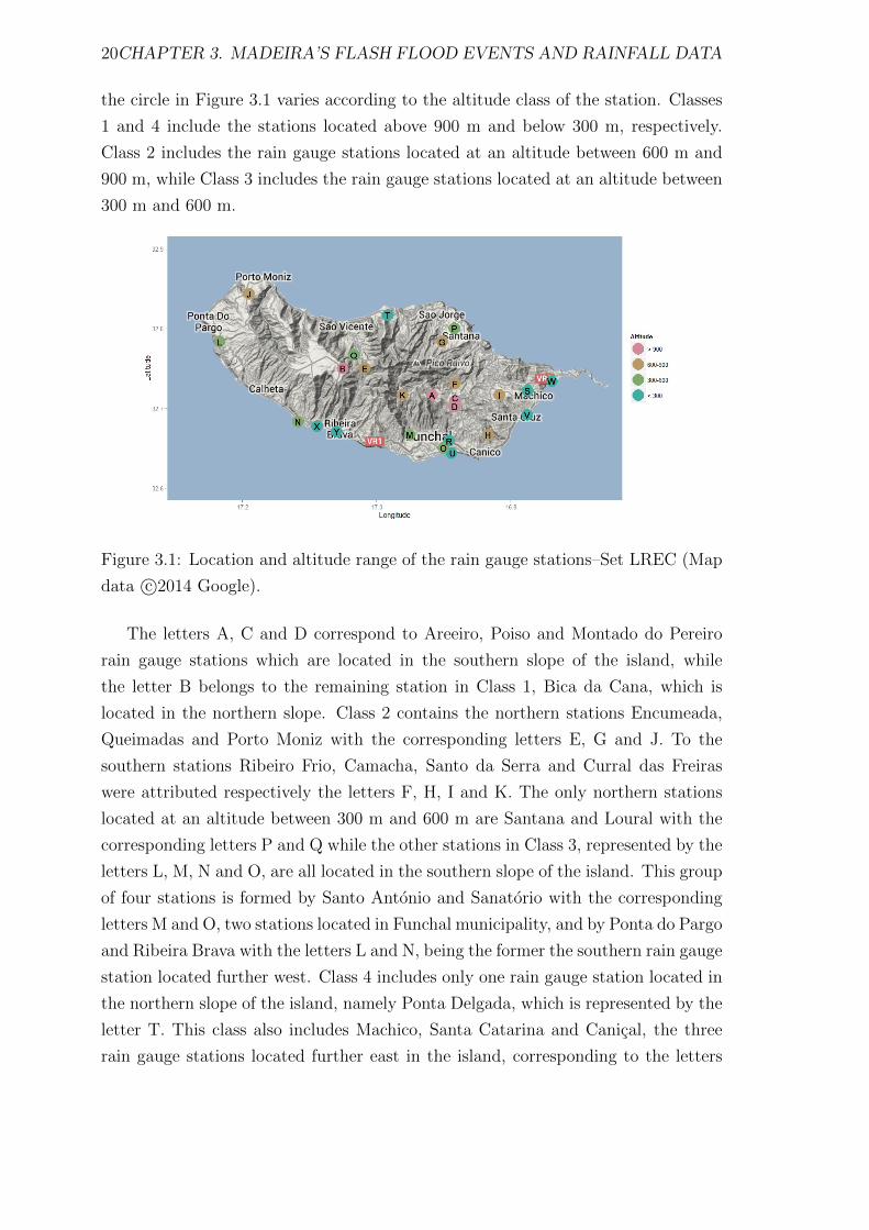
20CHAPTER 3. MADEIRA’S FLASH FLOOD EVENTS AND RAINFALL DATA
the circle in Figure 3.1 varies according to the altitude class of the station. Classes
1 and 4 include the stations located above 900 m and below 300 m, respectively.
Class 2 includes the rain gauge stations located at an altitude between 600 m and
900 m, while Class 3 includes the rain gauge stations located at an altitude between
300 m and 600 m.
Figure 3.1: Location and altitude range of the rain gauge stations–Set LREC (Map
data c©2014 Google).
The letters A, C and D correspond to Areeiro, Poiso and Montado do Pereiro
rain gauge stations which are located in the southern slope of the island, while
the letter B belongs to the remaining station in Class 1, Bica da Cana, which is
located in the northern slope. Class 2 contains the northern stations Encumeada,
Queimadas and Porto Moniz with the corresponding letters E, G and J. To the
southern stations Ribeiro Frio, Camacha, Santo da Serra and Curral das Freiras
were attributed respectively the letters F, H, I and K. The only northern stations
located at an altitude between 300 m and 600 m are Santana and Loural with the
corresponding letters P and Q while the other stations in Class 3, represented by the
letters L, M, N and O, are all located in the southern slope of the island. This group
of four stations is formed by Santo Antonio and Sanatorio with the corresponding
letters M and O, two stations located in Funchal municipality, and by Ponta do Pargo
and Ribeira Brava with the letters L and N, being the former the southern rain gauge
station located further west. Class 4 includes only one rain gauge station located in
the northern slope of the island, namely Ponta Delgada, which is represented by the
letter T. This class also includes Machico, Santa Catarina and Canical, the three
rain gauge stations located further east in the island, corresponding to the letters
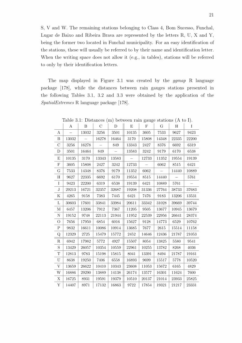
21
S, V and W. The remaining stations belonging to Class 4, Bom Sucesso, Funchal,
Lugar de Baixo and Ribeira Brava are represented by the letters R, U, X and Y,
being the former two located in Funchal municipality. For an easy identification of
the stations, these will usually be referred to by their name and identification letter.
When the writing space does not allow it (e.g., in tables), stations will be referred
to only by their identification letters.
The map displayed in Figure 3.1 was created by the ggmap R language
package [178], while the distances between rain gauges stations presented in
the following Tables 3.1, 3.2 and 3.3 were obtained by the application of the
SpatialExtremes R language package [178].
Table 3.1: Distances (m) between rain gauge stations (A to I).A B C D E F G H I
A − 13032 3256 3501 10135 3605 7533 9627 9423
B 13032 − 16278 16464 3170 15808 14348 22335 22200
C 3256 16278 − 849 13343 2427 8376 6692 6319
D 3501 16464 849 − 13583 3242 9179 6170 6538
E 10135 3170 13343 13583 − 12733 11352 19554 19139
F 3605 15808 2427 3242 12733 − 6062 8515 6421
G 7533 14348 8376 9179 11352 6062 − 14440 10889
H 9627 22335 6692 6170 19554 8515 14440 − 5761
I 9423 22200 6319 6538 19139 6421 10889 5761 −J 29213 16721 32357 32687 19208 31336 27764 38733 37683
K 4265 9158 7383 7445 6421 7476 9183 13206 13531
L 30603 17601 33841 33984 20611 33342 31028 39669 39744
M 6457 13206 7912 7367 11205 9505 13677 10945 13679
N 19152 9748 22113 21944 11952 22539 22956 26641 28374
O 7656 17950 6854 6016 15627 9128 14773 6529 10762
P 9832 16611 10086 10914 13685 7677 2615 15514 11158
Q 12329 2725 15479 15772 2452 14646 12436 21787 21053
R 6942 17982 5772 4927 15507 8054 13825 5580 9541
S 13429 26057 10354 10559 22961 10255 13782 8268 4036
T 12813 9783 15198 15815 8041 13391 8494 21787 19161
U 8638 19250 7406 6558 16893 9699 15517 5778 10520
V 13659 26622 10410 10343 23608 11053 15672 6165 4829
W 16886 29290 13889 14138 26174 13577 16301 11624 7600
X 16725 8931 19591 19379 10510 20137 21014 23933 25825
Y 14407 8971 17132 16863 9722 17854 19321 21217 23331
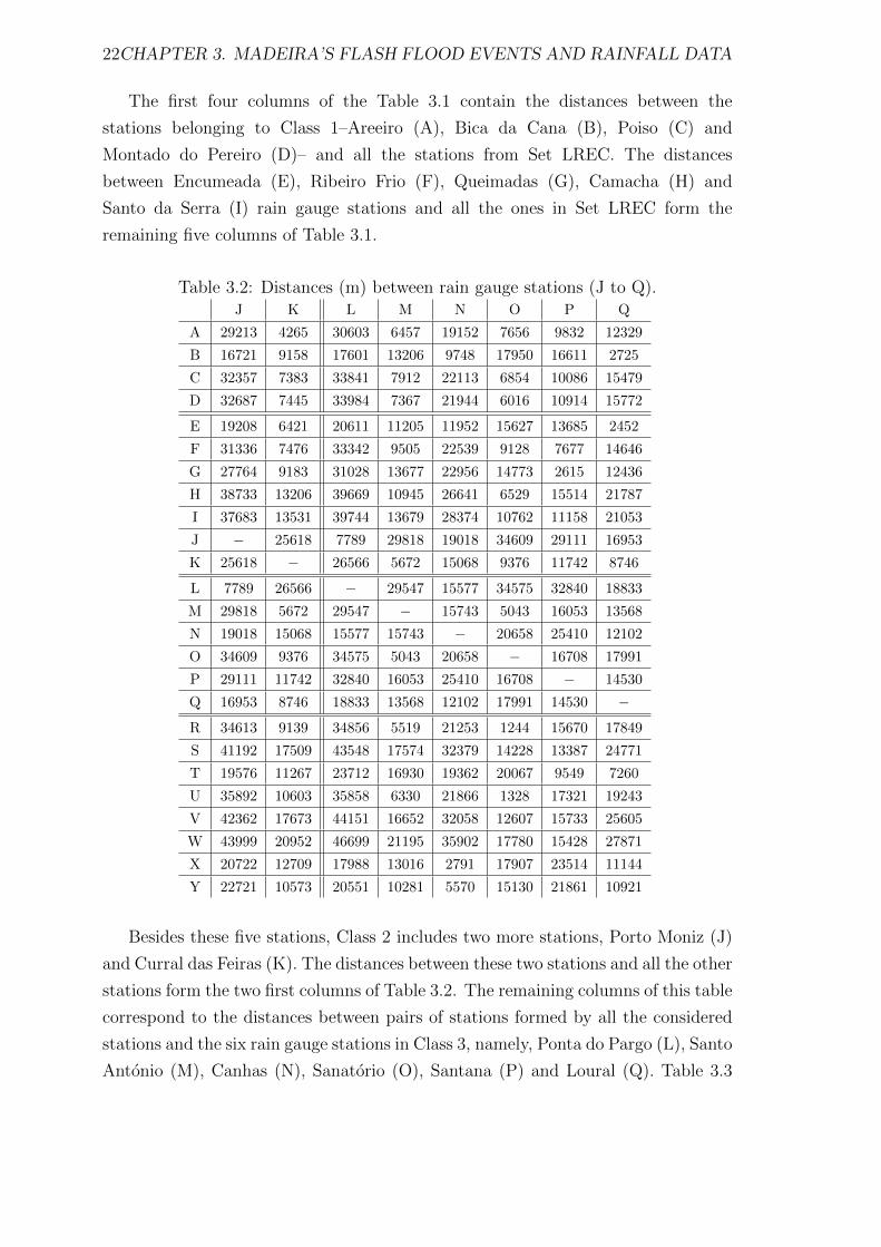
22CHAPTER 3. MADEIRA’S FLASH FLOOD EVENTS AND RAINFALL DATA
The first four columns of the Table 3.1 contain the distances between the
stations belonging to Class 1–Areeiro (A), Bica da Cana (B), Poiso (C) and
Montado do Pereiro (D)– and all the stations from Set LREC. The distances
between Encumeada (E), Ribeiro Frio (F), Queimadas (G), Camacha (H) and
Santo da Serra (I) rain gauge stations and all the ones in Set LREC form the
remaining five columns of Table 3.1.
Table 3.2: Distances (m) between rain gauge stations (J to Q).J K L M N O P Q
A 29213 4265 30603 6457 19152 7656 9832 12329
B 16721 9158 17601 13206 9748 17950 16611 2725
C 32357 7383 33841 7912 22113 6854 10086 15479
D 32687 7445 33984 7367 21944 6016 10914 15772
E 19208 6421 20611 11205 11952 15627 13685 2452
F 31336 7476 33342 9505 22539 9128 7677 14646
G 27764 9183 31028 13677 22956 14773 2615 12436
H 38733 13206 39669 10945 26641 6529 15514 21787
I 37683 13531 39744 13679 28374 10762 11158 21053
J − 25618 7789 29818 19018 34609 29111 16953
K 25618 − 26566 5672 15068 9376 11742 8746
L 7789 26566 − 29547 15577 34575 32840 18833
M 29818 5672 29547 − 15743 5043 16053 13568
N 19018 15068 15577 15743 − 20658 25410 12102
O 34609 9376 34575 5043 20658 − 16708 17991
P 29111 11742 32840 16053 25410 16708 − 14530
Q 16953 8746 18833 13568 12102 17991 14530 −
R 34613 9139 34856 5519 21253 1244 15670 17849
S 41192 17509 43548 17574 32379 14228 13387 24771
T 19576 11267 23712 16930 19362 20067 9549 7260
U 35892 10603 35858 6330 21866 1328 17321 19243
V 42362 17673 44151 16652 32058 12607 15733 25605
W 43999 20952 46699 21195 35902 17780 15428 27871
X 20722 12709 17988 13016 2791 17907 23514 11144
Y 22721 10573 20551 10281 5570 15130 21861 10921
Besides these five stations, Class 2 includes two more stations, Porto Moniz (J)
and Curral das Feiras (K). The distances between these two stations and all the other
stations form the two first columns of Table 3.2. The remaining columns of this table
correspond to the distances between pairs of stations formed by all the considered
stations and the six rain gauge stations in Class 3, namely, Ponta do Pargo (L), Santo
Antonio (M), Canhas (N), Sanatorio (O), Santana (P) and Loural (Q). Table 3.3

23
presents the distances between Bom Sucesso (R), Machico (S), Ponta Delgada (T),
Funchal (U), Santa Catarina (V), Canical (W), Lugar de Baixo (X) and Ribeira
Brava (Y), and all the rain gauge stations in Set LREC.
Table 3.3: Distances (m) between rain gauge stations (R to Y).R S T U V W X Y
A 6942 13429 12813 8638 13659 16886 16725 14407
B 17982 26057 9783 19250 26622 29290 8931 8971
C 5772 10354 15198 7406 10410 13889 19591 17132
D 4927 10559 15815 6558 10343 14138 19379 16863
E 15507 22961 8041 16893 23608 26174 10510 9722
F 8054 10255 13391 9699 11053 13577 20137 17854
G 13825 13782 8494 15517 15672 16301 21014 19321
H 5580 8268 21787 5778 6165 11624 23933 21217
I 9542 4036 19161 10520 4829 7600 25825 23331
J 34613 41192 19576 35892 42362 43999 20722 22721
K 9139 17509 11267 10603 17673 20952 12709 10573
L 34856 43548 23712 35858 44151 46699 17988 20551
M 5519 17574 16930 6330 16652 21195 13016 10281
N 21253 32379 19362 21866 32058 35902 2791 5570
O 1244 14228 20067 1328 12607 17780 17907 15130
P 15670 13387 9549 17321 15733 15428 23514 21861
Q 17849 24771 7260 19243 25605 27871 11144 10921
R − 13055 19483 1712 11558 16625 18513 15761
S 13055 − 22218 13750 3358 3622 29822 27319
T 19483 22218 − 21129 23944 24707 18291 17685
U 1712 13750 21129 − 11877 17238 19104 16319
V 11558 3358 23944 11877 − 5803 29402 26770
W 16625 3622 24707 17238 5803 − 33369 30893
X 18513 29822 18291 19104 29402 33369 − 2795
Y 15761 27319 17685 16319 26770 30893 2795 −
For each rain gauge station in Set LREC, the station’s name and identification
letter, geographical location, altitude and the measurement period considered are
presented in Table 3.4. The island slope where each one of the mentioned rain gauge
stations is located is also shown in Table 3.4, with 1 denoting the northern slope
and 2 the southern one. For a quick identification of all the rain gauge stations
within a specific class of altitude, there are three extra horizontal lines in Table 3.4
separating the stations that are included in Classes 1, 2, 3 and 4.
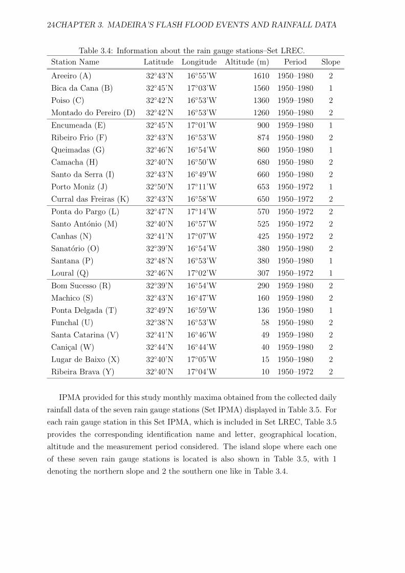
24CHAPTER 3. MADEIRA’S FLASH FLOOD EVENTS AND RAINFALL DATA
Table 3.4: Information about the rain gauge stations–Set LREC.
Station Name Latitude Longitude Altitude (m) Period Slope
Areeiro (A) 32◦43’N 16◦55’W 1610 1950–1980 2
Bica da Cana (B) 32◦45’N 17◦03’W 1560 1950–1980 1
Poiso (C) 32◦42’N 16◦53’W 1360 1959–1980 2
Montado do Pereiro (D) 32◦42’N 16◦53’W 1260 1950–1980 2
Encumeada (E) 32◦45’N 17◦01’W 900 1959–1980 1
Ribeiro Frio (F) 32◦43’N 16◦53’W 874 1950–1980 2
Queimadas (G) 32◦46’N 16◦54’W 860 1950–1980 1
Camacha (H) 32◦40’N 16◦50’W 680 1950–1980 2
Santo da Serra (I) 32◦43’N 16◦49’W 660 1950–1980 2
Porto Moniz (J) 32◦50’N 17◦11’W 653 1950–1972 1
Curral das Freiras (K) 32◦43’N 16◦58’W 650 1950–1972 2
Ponta do Pargo (L) 32◦47’N 17◦14’W 570 1950–1972 2
Santo Antonio (M) 32◦40’N 16◦57’W 525 1950–1972 2
Canhas (N) 32◦41’N 17◦07’W 425 1950–1972 2
Sanatorio (O) 32◦39’N 16◦54’W 380 1950–1980 2
Santana (P) 32◦48’N 16◦53’W 380 1950–1980 1
Loural (Q) 32◦46’N 17◦02’W 307 1950–1972 1
Bom Sucesso (R) 32◦39’N 16◦54’W 290 1959–1980 2
Machico (S) 32◦43’N 16◦47’W 160 1959–1980 2
Ponta Delgada (T) 32◦49’N 16◦59’W 136 1950–1980 1
Funchal (U) 32◦38’N 16◦53’W 58 1950–1980 2
Santa Catarina (V) 32◦41’N 16◦46’W 49 1959–1980 2
Canical (W) 32◦44’N 16◦44’W 40 1959–1980 2
Lugar de Baixo (X) 32◦40’N 17◦05’W 15 1950–1980 2
Ribeira Brava (Y) 32◦40’N 17◦04’W 10 1950–1972 2
IPMA provided for this study monthly maxima obtained from the collected daily
rainfall data of the seven rain gauge stations (Set IPMA) displayed in Table 3.5. For
each rain gauge station in this Set IPMA, which is included in Set LREC, Table 3.5
provides the corresponding identification name and letter, geographical location,
altitude and the measurement period considered. The island slope where each one
of these seven rain gauge stations is located is also shown in Table 3.5, with 1
denoting the northern slope and 2 the southern one like in Table 3.4.
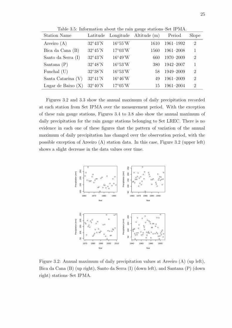
25
Table 3.5: Information about the rain gauge stations–Set IPMA.
Station Name Latitude Longitude Altitude (m) Period Slope
Areeiro (A) 32◦43’N 16◦55’W 1610 1961–1992 2
Bica da Cana (B) 32◦45’N 17◦03’W 1560 1961–2008 1
Santo da Serra (I) 32◦43’N 16◦49’W 660 1970–2009 2
Santana (P) 32◦48’N 16◦53’W 380 1942–2007 1
Funchal (U) 32◦38’N 16◦53’W 58 1949–2009 2
Santa Catarina (V) 32◦41’N 16◦46’W 49 1961–2009 2
Lugar de Baixo (X) 32◦40’N 17◦05’W 15 1961–2004 2
Figures 3.2 and 3.3 show the annual maximum of daily precipitation recorded
at each station from Set IPMA over the measurement period. With the exception
of these rain gauge stations, Figures 3.4 to 3.8 also show the annual maximum of
daily precipitation for the rain gauge stations belonging to Set LREC. There is no
evidence in each one of these figures that the pattern of variation of the annual
maximum of daily precipitation has changed over the observation period, with the
possible exception of Areeiro (A) station data. In this case, Figure 3.2 (upper left)
shows a slight decrease in the data values over time.
1960 1970 1980 1990
100
150
200
250
Year
Pre
cipi
tatio
n (m
m)
1960 1970 1980 1990 2000
5010
015
020
025
0
Year
Pre
cipi
tatio
n (m
m)
1970 1980 1990 2000 2010
5010
015
020
025
0
Year
Pre
cipi
tatio
n (m
m)
1940 1960 1980 2000
5010
015
020
0
Year
Pre
cipi
tatio
n (m
m)
Figure 3.2: Annual maximum of daily precipitation values at Areeiro (A) (up left),
Bica da Cana (B) (up right), Santo da Serra (I) (down left), and Santana (P) (down
right) stations–Set IPMA.

26CHAPTER 3. MADEIRA’S FLASH FLOOD EVENTS AND RAINFALL DATA
1950 1970 1990 2010
2060
100
Year
Pre
cipi
tatio
n (m
m)
1960 1980 2000
4080
120
Year
Pre
cipi
tatio
n (m
m)
1960 1980 2000
4080
120
Year
Pre
cipi
tatio
n (m
m)
Figure 3.3: Annual maximum of daily precipitation values at Funchal (U) (up left),
Santa Catarina (V) (up right), and Lugar de Baixo (X) (down) stations–Set IPMA.
1960 1970 1980
100
150
200
250
Year
Pre
cipi
tatio
n (m
m)
1950 1960 1970 1980
100
150
200
250
Year
Pre
cipi
tatio
n (m
m)
1960 1970 1980
100
200
Year
Pre
cipi
tatio
n (m
m)
1950 1960 1970 1980
100
150
200
Year
Pre
cipi
tatio
n (m
m)
Figure 3.4: Annual maximum of daily precipitation values at Poiso (C) (up left),
Montado do Pereiro (D) (up right), Encumeada (E) (down left), and Ribeiro Frio (F)
(down right) stations–Set LREC.

27
1950 1960 1970 1980
6010
014
018
0
Year
Pre
cipi
tatio
n (m
m)
1950 1960 1970 1980
6010
014
018
0
Year
Pre
cipi
tatio
n (m
m)
1950 1960 1970
5010
020
0
Year
Pre
cipi
tatio
n (m
m)
Figure 3.5: Annual maximum of daily precipitation values at Queimadas (G)
(up left), Camacha (H) (up right), and Porto Moniz (J) (down) stations–Set LREC.
1950 1960 1970
8012
016
020
0
Year
Pre
cipi
tatio
n (m
m)
1950 1960 1970
4060
8012
0
Year
Pre
cipi
tatio
n (m
m)
1950 1960 1970
4080
120
Year
Pre
cipi
tatio
n (m
m)
1950 1960 1970
6080
100
Year
Pre
cipi
tatio
n (m
m)
Figure 3.6: Annual maximum of daily precipitation values at Curral das Freiras (K)
(up left), Ponta do Pargo (L) (up right), Santo Antonio (M) (down left), and
Canhas (N) (down right) stations–Set LREC.
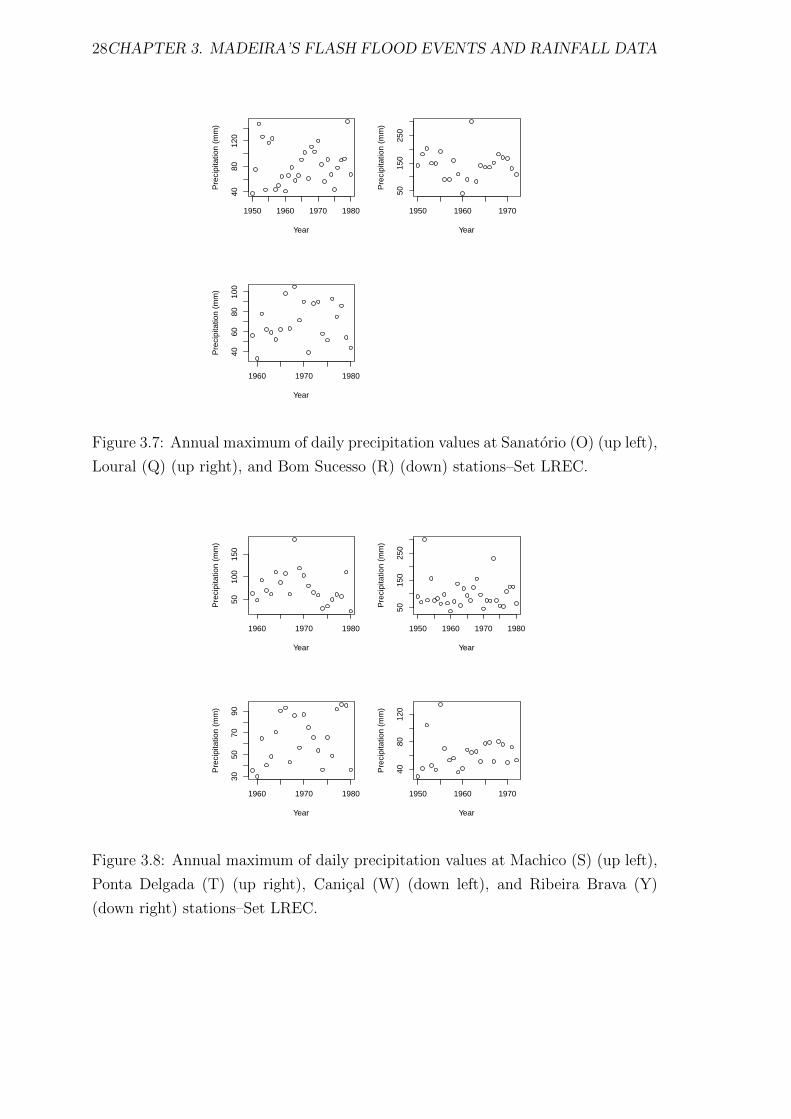
28CHAPTER 3. MADEIRA’S FLASH FLOOD EVENTS AND RAINFALL DATA
1950 1960 1970 1980
4080
120
Year
Pre
cipi
tatio
n (m
m)
1950 1960 1970
5015
025
0
Year
Pre
cipi
tatio
n (m
m)
1960 1970 1980
4060
8010
0
Year
Pre
cipi
tatio
n (m
m)
Figure 3.7: Annual maximum of daily precipitation values at Sanatorio (O) (up left),
Loural (Q) (up right), and Bom Sucesso (R) (down) stations–Set LREC.
1960 1970 1980
5010
015
0
Year
Pre
cipi
tatio
n (m
m)
1950 1960 1970 1980
5015
025
0
Year
Pre
cipi
tatio
n (m
m)
1960 1970 1980
3050
7090
Year
Pre
cipi
tatio
n (m
m)
1950 1960 1970
4080
120
Year
Pre
cipi
tatio
n (m
m)
Figure 3.8: Annual maximum of daily precipitation values at Machico (S) (up left),
Ponta Delgada (T) (up right), Canical (W) (down left), and Ribeira Brava (Y)
(down right) stations–Set LREC.
Chapter 4
Methodology
4.1 Gumbel’s model approach
The present section is related to the univariate extreme value theory, especially to
the so called Gumbel’s approach. The opening subsection recalls the generalised
and also the standard extreme value distributions, while the second one presents
the parameter estimation methods and statistical tests applied in Section 5.1 of
Chapter 5. The model checking procedures used in this thesis are presented in
subsection 4.1.3. Subsection 4.1.4 concludes the section. In this subsection, the
models considered in the trend analysis of Madeira Island’s annual rainfall data are
presented.
One method of extracting upper extremes from a set of data is called annual
maxima, blocks or Gumbel method. In this method, the considered dataset is
organised in blocks of equal size – assume that there are n blocks of size m – from
which the maximum values are chosen:
xi = max{yi,1, ..., yi,m}, i = 1, ..., n.
To implement this model a block size choice is needed, which implies an
underlying trade-off between bias and variance. A large block size yields few
block maxima and consequently large estimation variance. On the other hand, a
small block size can lead to a poor limit model approximation. Addressing this
problem, blocks are often chosen to correspond to a time period of one year, being
m the number of observations in a year and, therefore, block maxima being annual
maxima [26].
29
30 CHAPTER 4. METHODOLOGY
Let X1, X2, ..., Xn be independent random variables with a common distribution
function F . The distribution function of the maximum is given by
P
{maxi≤n
Xi ≤ x
}= P{X1 ≤ x, ..., Xn ≤ x} = F n(x).
It is important to notice that a distribution function of the form F n may still be
an accurate approximation of the actual distribution of the maximum, even when
the conditions of independence and homogeneity fail. When the variables Xi are
independent but heterogeneous with distribution functions Fi, Fn is replaced by∏
j≤n Fj. The distribution function F n can still be used instead of∏
j≤n Fj if the
deviations between the different distribution functions are negligible. On the other
hand, even if there is a slight dependence in the data, a distribution function of
the form F n may still be considered as a good approximation of the distribution
function of the maximum [179].
4.1.1 Extreme value distributions
The distribution of the largest extreme values in hydrology generally appears as a
type I extreme value distribution since most hydrologic variables are unbounded on
the right. Type I extreme value distribution is also referred to as the Gumbel’s
extreme value distribution, the Fisher–Tippett type I distribution, and the double
exponential distribution. Besides Gumbel’s extreme value distribution, there are two
other extreme value distributions, the Fisher-Tippett types II and III distributions,
also known as the Frechet and the Weibull distribution functions.
The three standard extreme value distribution functions are defined in the
following way, for x ∈ R:
• Gumbel (EV0): G0(x) = exp(− exp(−x)),
• Frechet (EV1), α > 0: G1,α (x) = exp (−x−α) IR+0
(x),
• Weibull (EV2), α < 0: G2,α (x) = exp(− (−x)−α
)IR− (x) + IR+
0(x).
Besides the above terminologies, the Gumbel distribution is also represented
in the literature by the Greek letter Λ, while the Frechet distribution with shape
parameter α > 0 is represented by Φα, and the Weibull distribution function by Ψα,
where α < 0 [179].
4.1. GUMBEL’S MODEL APPROACH 31
A unified model, known as the GEV distribution, is obtained through the von
Mises’ parametrization [219]. This model, which is also frequently attributed to
Jenkinson [121], is defined for γ = 1α
in the following way:
Gγ(x) =
{exp(−(1 + γx)−1/γ), if 1 + γx > 0, γ 6= 0;
exp(− exp(−x)), if x ∈ R, γ = 0.(4.1)
By adding location and scale parameters, µ and σ > 0, the full GEV family
Gγ(x−µσ
) follows. This unified model allows a unified expression also for the return
levels. For a given small probability p, a return level is a threshold qp, whose
probability of exceedance is p. In the context of annual block maxima, the return
level is the value exceeded by the annual maximum in any particular year with
probability p. In other words, the return level qp is the value expected to be exceeded
once every 1/p years [26].
Return level estimates qp can be obtained by the estimation of the extreme
quantiles of the annual maximum distribution given by
qp =
{µ− σ
γ[1− (− log(1− p))−γ], if γ 6= 0;
µ− σ log (− log(1− p)), if γ = 0,(4.2)
where µ, σ and γ are replaced by their respective estimates.
The use of Frechet, Weibull and Gumbel distribution functions in the modelling
of maxima is justified by the works of Frechet [71], Fisher and Tippet [66],
Gnedenko [83] and de Haan [39]. Together, these authors have found these
distributions to be the possible non-degenerate limits of sequences F n (bn + anx),
when n → +∞, for some sequences of constants bn and an > 0. The same authors
have also found the sufficient and necessary conditions on the distribution function
F for the convergence to these limits (see, e.g., J. Galambos [76]). In short, if
F n(bn + anx) has a non-degenerate limiting distribution function as n → ∞ for
constants bn and an > 0, then∣∣∣∣F n(bn + anx)−G(x− µσ
)∣∣∣∣→ 0, n→∞
with G ∈ {G0, G1,α, G2,−α, for some α ∈ R+} or, equivalently, G = Gγ, for some
γ ∈ R, where µ and σ > 0 are the location and scale parameters, respectively.
It is important to notice that the behaviour of the right tail of the distribution
function F determines the limit distribution of the normalised maximum (see, e.g.,
J. Galambos [76]). Even the right endpoint of the support of F has some influence,
32 CHAPTER 4. METHODOLOGY
for a finite one excludes as limit distribution the ones from the Frechet family and
an infinite one excludes the distributions from the Weibull family.
4.1.2 Parameter estimation methods and statistical tests
A variety of estimation methods for the extreme value distributions parameters
are present in the literature, such as, for example, the method of moments, the
ML and the PWM methods (see, e.g. [10, 21, 128]). The ML method is based on
maximising the likelihood of the observed sample, while the moments estimators
are obtained by comparing moments of the random variable to the corresponding
sample moments. The PWM method is a variant of the latter method, which
was introduced in 1979 by Greenwood et al. [98]. In the same year, Landwehr et
al. [133] proposed the use of this method for extreme value distributions. According
to Embrechts et al. [61], the method of moments attracted a lot of interest among
the researchers. For example, in 1958, Gumbel [107] preferred this method and
argued that the ML method required too much numerical work for routine use.
However, in 1982, Lettenmaier and Burges [137] showed that the ML method gave
better parameter estimates than the ones given by the method of moments. In
fact, Lettenmaier and Burges [137] paper is one among many papers found in
the literature devoted to the ML estimation [128]. The big advantage of the ML
method is to allow the study of more complex situations as non–stationarity and
covariate effects [28], without the need of a lot of changes in the basic methodology
of its procedures [61]. On the other hand, the major disadvantage of the ML
method is that it can be extremely erratic for small samples, contrary to what
happens with the PWM method [124]. The latter method is also a popular one in
extreme value investigations, and especially in environmental sciences [128], having
in its favour the simplicity of application and a good performance in simulation
studies [61]. In 1979, Landwehr et al. [133] addressed the comparability between
the PWM method and the two methods applied extensively in hydrology at that
time, ML and moments methods, arriving to the conclusion that for the Gumbel
distribution the results obtained with the PWM method were favourably compared
with those for the two older methods. However, as mentioned by Embrechts et
al. [61] in 1997, the PWM method has the disadvantage of not yet being extended
to more complex situations. Despite their advantages and disadvantages, both
methods can be applied in a complementary way since the PWM method can be
used to provide initial values for the iterative numerical procedure that leads to the
ML estimates [124].

4.1. GUMBEL’S MODEL APPROACH 33
ML method
The ML estimator (σ, γ, µ) for (σ, γ, µ) is obtained by maximising the log-likelihood
function. Given a sample X1, ..., Xn of independent and identically distributed
random variables with common GEV distribution defined by expression (4.1), this
function is given, when γ 6= 0, by
logL(σ, γ, µ) = −n log σ−(
1
γ+ 1
) n∑i=1
log
(1 + γ
Xi − µσ
)−
n∑i=1
(1 + γ
Xi − µσ
) 1γ
,
provided 1 + γXi−µσ
> 0, i = 1, ..., n. In case γ = 0, the log-likelihood function
reduces to
logL(σ, 0, µ) = −n log σ −n∑i=1
exp
(Xi − µσ
)−
n∑i=1
(Xi − µσ
).
Confidence intervals concerning the GEV parameters (σ, γ, µ) follow from the
asymptotic normality of the ML estimators. For example, for α ∈ (0, 1) the
(1− α)100% confidence interval for γ is given by
(γ − z1−α
2
√v2,2n, γ + z1−α
2
√v2,2n
)(4.3)
with γ the ML estimate of γ, z1−α2
the (1− α2)–quantile of the normal distribution
and v2,2 the second diagonal element of the inverse of the Fisher information matrix,
which is defined by
I(θ) = −E(∂2 log g(X; θ)
∂θ∂θ′
),
with θ = (σ, γ, µ) and g the GEV density function
g(x;σ, γ, µ) =1
σ
(1 + γ
x− µσ
)exp
(−(
1 + γx− µσ
)− 1γ
).
34 CHAPTER 4. METHODOLOGY
The Fisher information matrix has as generic elements
I1,1(θ) =1
σ2γ2(1− 2Γ(2 + γ) + a),
I1,2(θ) = − 1
σγ2
(1− ε− b+
1− Γ(2 + γ)
γ+a
γ
),
I1,3(θ) =1
σ2γ(a− Γ(2 + γ)),
I2,2(θ) =1
γ2
[π2
6+
(1− ε+
1
γ
)− 2b
γ+
a
γ2
],
I2,3(θ) = − 1
σγ
(b− a
γ
),
I3,3(θ) =a
σ2,
where ε ≈ 0.5772157 is Euler’s constant,
a = (1 + γ)2Γ(1 + 2γ),
b = Γ(2 + γ)
(ψ(1 + γ) +
1 + γ
γ
),
with ψ(x) = d log Γ(x)/dx [10]. The greek letter Γ stands, as usual, for the gamma
function defined by
Γ(t) =
∫ +∞
0
exp (−x)xt−1dx, for t > 0. (4.4)
Nevertheless, it is important to have in mind that inference based on the normal
limit results may be misleading as the normal approximation to the true sampled
distribution of the corresponding estimator can be poor [10]. In general, better
approximations can be obtained by the profile likelihood function as the confidence
intervals obtained in this way are not necessarily centred in the corresponding point
estimates as the ones resulting from the normality approximation [10, 87]. More
explicitly, profile likelihood intervals may present a shift to the right while the ones
resulting from the normality approximation are always centred in the corresponding
point estimates due the symmetry presented by the normal distribution (see,
e.g., [26, 87]).
The profile likelihood function for γ is given by
Lp(γ) = max(σ,µ)|γ
L(σ, γ, µ),
4.1. GUMBEL’S MODEL APPROACH 35
and the profile likelihood ratio statistic by
R =Lp(γ0)
Lp(γ),
which coincides with the classical likelihood ratio statistic for testing the hypothesis
H0 : γ = γ0 versus H1 : γ 6= γ0. Hence, under H0, when n→∞,
−2 logRd−→ χ2
1,
whered−→ stands for “converges in distribution to” and χ2
1 for the qui–square
distribution with one degree of freedom. The null hypothesis H0 will be rejected
at a significance level of α if −2 logR > χ21(1 − α), where χ2
1(1 − α) is the
(1 − α)–quantile of the χ21 distribution. Consequently, the profile likelihood-based
(1− α)100% confidence interval for γ is given by
CIγ =
{γ : −2 log
Lp(γ)
Lp(γ)≤ χ2
1(1− α)
}or equivalently
CIγ =
{γ : logLp(γ) ≥ logLp(γ)− χ2
1(1− α)
2
}.
PWM method
The test of the so–called Gumbel hypothesis (H0 : γ = 0), can also be based on the
PWM estimate of γ presented by Hosking et al. [119]. Given a random variable X
with distribution function F , the PWM of X are defined as
Mm,r,s = E [Xm {F (X)}r {1− F (X)}s] ,
where m, r, s ∈ R (cf., e.g., [119]). The PWM generalise the noncentral moments of
X, E (Xm), which are obtained when r = s = 0 and m = 1, 2, .... When s ∈ N1,
{1− F (x)}s =s∑j=0
(s
j
)[−F (x)]j
and
Mm,r,s = E [Xm {F (X)}r {1− F (X)}s] =s∑j=0
(s
j
)(−1)jMm,r+j,0,
and though special attention is given to the moments Mm,r,0 (a similar reasoning
can be made for r ∈ N1).
36 CHAPTER 4. METHODOLOGY
Consider X with distribution function given by Gγ
(•−µσ
)where Gγ is the GEV
distribution with expression given by (4.1). It is not difficult to prove that
M1,r,0 =1
r + 1
(µ− σ
γ(1− (r + 1)γΓ(1− γ))
), (4.5)
for γ < 1, taking into account that when F is an injective function,
Mm,r,s =
∫Rxm {F (x)}r {1− F (x)}s dF (x)
=
∫ 1
0
[F−1 (y)
]myr (1− y)s dy,
where F−1(y) = q1−y, and qp is given by expression (4.2). The greek letter Γ stands
as before for the gamma function defined by (4.4).
The PWM estimators of γ, σ and µ (σ, γ, µ) are the solutions of the following
system of equations obtained from (4.5) taking r = 0, 1, 2, after M1,r,0 is replaced
by an appropriate estimator:M1,0,0 = µ− σ
γ(1− Γ(1− γ)),
2M1,1,0 −M1,0,0 = σγΓ(1− γ)(2γ − 1)
3M1,2,0 −M1,0,0
2M1,1,0 −M1,0,0
=3γ − 1
2γ − 1
. (4.6)
The system above is solved after replacing M1,r,0 by, for example, the estimator
proposed by Landwehr et al. [133]:
M1,r,0 =1
n
n∑j=1
(r∏l=1
(j − l)(n− l)
)Xj:n.
The third equation in system (4.6) is solved numerically to obtain γ and, using this
result, the second equation in system (4.6) is solved for σ:
σ =γ(2M1,1,0 − M1,0,0)
Γ(1− γ)(2γ − 1).
Finally, µ is obtained through the first equation in system (4.6)
µ = M1,0,0 +σ
γ(1− Γ(1− σ)).
The test based on the PWM estimator of γ proposed by Hosking et al. [119] is
performed by comparing the test statistic
γ( n
0.5633
) 12
(4.7)
with the critical values of the standard normal distribution.
4.1. GUMBEL’S MODEL APPROACH 37
4.1.3 Plots and statistical tests for model diagnostics
After having found the estimates for the parameters, the adequacy of a Gumbel or
a non-Gumbel model can be checked through probability, quantile and return level
plots, which are based on a comparison of model–based and empirical estimates of
the distribution function [26]. The GEV distribution defined in (4.1) with µ as the
location parameter, σ as the scale parameter and γ as the shape parameter will be
from now on denoted by GEV (µ, σ, γ), and referred to as Model 1 when γ 6= 0. The
particular case of γ = 0 in (4.1) will be designated as Model 2 (GEV (µ, σ, 0)).
Let x1:n, ..., xn:n be the ordered sample of the block maxima x1, ..., xn. The
empirical distribution function at xi:n is
G(xi:n) =i
n+ 1,
and
G(xi:n) = exp
{−[1 + γ
(xi:n − µ
σ
)]−1/γ}, i = 1, . . . , n,
are the GEV model-based estimates, where γ, µ and σ are estimates for γ, µ and σ,
respectively. The probability plot consists of the points(G(xi:n), G(xi:n)
), i = 1, . . . , n,
which are expected to lie close to the diagonal {(x, x), x ∈ [0, 1]} if Model 1 is
adequate. For the highest values of xi:n, both G(xi:n) and G(xi:n) are, by definition,
close to one, which may be misleading in the interpretation of the region of major
interest. Therefore, the analysis of this plot should be complemented with the one
resulting from the quantile plot defined by the points(G−1
(i
n+ 1
), xi:n
), i = 1, . . . , n,
where by (4.2)
G−1(
i
n+ 1
)= µ− σ
γ
[1−
(− log
(i
n+ 1
)−γ)].
As it happened before with the probability plot, departures from linearity in
the quantile plot indicate that Model 1 is not an adequate model. Analogously,
probability and quantile plots can be used to check the adequacy of Model 2.
Considering again the return levels defined by (4.2), the return level plot consists
of the points
(log yp, qp), 0 < p < 1,
38 CHAPTER 4. METHODOLOGY
where yp = − log(1 − p). This plot is linear when Model 2 is an adequate choice,
being convex or concave for Model 1 particular cases of γ < 0 and γ > 0, respectively.
Also, when γ < 0, the graphical representation of the set {(log yp, qp) , p ∈ (0, 1)}has an asymptotic limit, as p → 0, equal to µ − σ/γ. When γ > 0, the graph is
unbounded when p → 0. The simplicity of the interpretation of these plots turns
these particularly important for both model presentation and validation.
To complement the information obtained by the previous analysis, confidence
intervals for the return level qp can be added. These are defined by(qp − z1−α
2
√V ar(qp), qp + z1−α
2
√V ar(qp)
)with z1−α
2the (1− α)–quantile of the standard normal distribution and V ar(qp) =
∇qTp V∇qp, where V is the variance–covariance matrix of (µ, σ, γ) and
∇qTp =
[∂qp∂µ
,∂qp∂σ
,∂qp∂γ
]=[1,−γ−1(1− y−γp ), σγ−2(1− y−γp )− σγ−1y−γp log yp
]evaluated at (µ, σ, γ) [26]. For example, the values qp can be obtained by substitution
of the ML estimates of the GEV parameters into (4.2), being its normality justified
by the delta method [10].1 The analysis of the adequacy of Model 1 and 2 through
the probability, quantile and return level plots can also be complemented with a
comparison between a histogram of the data and the probability density function
of the fitted model. The graphical approach to the analysis of the adequacy of
the model should be followed by a goodness of fit test such as the Kolmogorov–
Smirnov test. The evaluation of the adequacy of Model 2 can also be made by the
application of a goodness of fit test developed by Stephens [200]. This test is based
on the empirical distribution function statistic A2 defined by
1The delta method is the term usually attributed to the following theorem [26]: Let θ0 be
the large–sample ML estimator of the d–dimensional parameter θ0 with approximate variance–
covariance matrix Vθ. If Φ = g(θ) is a scalar function, then the ML estimator of Φ0 = g(θ0)
satisfies
Φ0 ≈ N(Φ0, VΦ)
where
VΦ = ∇ΦTVθ∇Φ
with
∇Φ =
[∂Φ
∂θ1, ...,
∂Φ
∂θd
]Tevaluated at θ0.

4.1. GUMBEL’S MODEL APPROACH 39
A2 = − 1
n
n∑i=1
(2i− 1) [log zi + log(1− zn+1−i)]− n (4.8)
where
zi = G(xi:n) = exp
[− exp
(xi:n − µ
σ
)]are the Gumbel model-based estimates obtained, for example, by substitution of
the parameters µ and σ by the PWM estimates µ and σ. For small samples,
Stephens [200] recommends the replacement of A2 by
A∗2 = A2
(1 +
0.2√n
). (4.9)
The obtained values for A2 or A∗2 can then be compared with the corresponding
upper tail points [Table 1 in [200]].
4.1.4 A trend analysis
Until now the random variables involved are assumed to be independent and to
have identical distributions, and both estimation methods, ML and PWM, were
considered. At the presence of non–stationarities, a usual aspect when a time series
is involved, the ML estimation method is the one that should be applied, as it
allows this aspect to be included in the analysis. According to Engeland et al. [62]
the non–stationarity can be accounted by three ways, namely, by a decomposition of
the time series into a deterministic seasonal component and a stationary sequence,
by a subdivision of the dataset into blocks that can be assumed homogeneous or by
the inclusion of parameters in the GEV distribution depending on the time or other
covariates. The Kruskal–Wallis test can be used to test the distributional identity of
the subsamples mentioned in the second approach (see, e.g., [132]). This approach
has the drawback of requiring the construction of the blocks. The third approach is
considered more flexible and was applied by a number of authors [26, 62, 154, e.g.].
This approach consists in the introduction of time dependence in the parameters
of the GEV distribution. The simplest way is to consider a linear trend although
according to Coles [26] there are many applications for which the variations through
time do not have the low order polynomial form. Coles [26] also advocates that is
usually unrealistic to try to model the shape parameter γ for it is difficult to obtain
a precise estimate for this one. Taking this into account, only location and scale
parameters are considered in the following trend analysis.
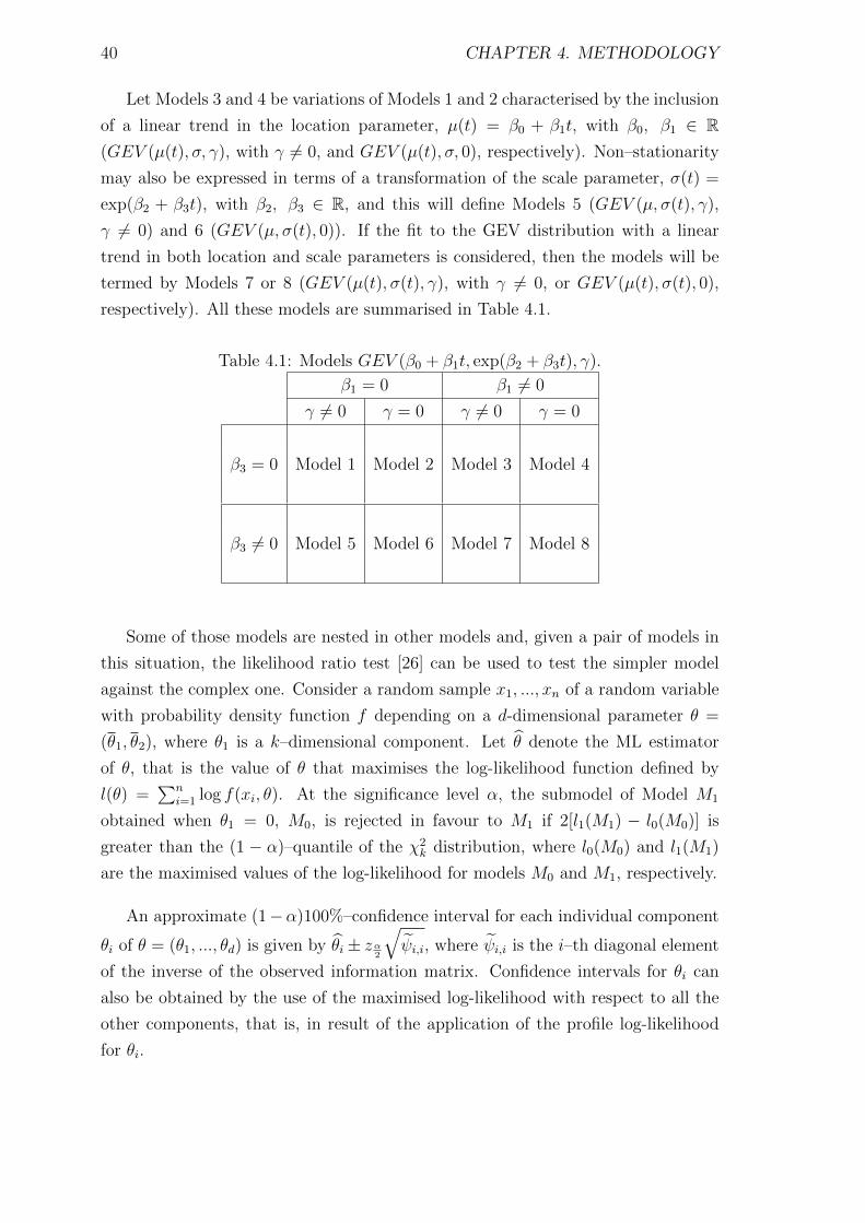
40 CHAPTER 4. METHODOLOGY
Let Models 3 and 4 be variations of Models 1 and 2 characterised by the inclusion
of a linear trend in the location parameter, µ(t) = β0 + β1t, with β0, β1 ∈ R(GEV (µ(t), σ, γ), with γ 6= 0, and GEV (µ(t), σ, 0), respectively). Non–stationarity
may also be expressed in terms of a transformation of the scale parameter, σ(t) =
exp(β2 + β3t), with β2, β3 ∈ R, and this will define Models 5 (GEV (µ, σ(t), γ),
γ 6= 0) and 6 (GEV (µ, σ(t), 0)). If the fit to the GEV distribution with a linear
trend in both location and scale parameters is considered, then the models will be
termed by Models 7 or 8 (GEV (µ(t), σ(t), γ), with γ 6= 0, or GEV (µ(t), σ(t), 0),
respectively). All these models are summarised in Table 4.1.
Table 4.1: Models GEV (β0 + β1t, exp(β2 + β3t), γ).
β1 = 0 β1 6= 0
γ 6= 0 γ = 0 γ 6= 0 γ = 0
β3 = 0 Model 1 Model 2 Model 3 Model 4
β3 6= 0 Model 5 Model 6 Model 7 Model 8
Some of those models are nested in other models and, given a pair of models in
this situation, the likelihood ratio test [26] can be used to test the simpler model
against the complex one. Consider a random sample x1, ..., xn of a random variable
with probability density function f depending on a d-dimensional parameter θ =
(θ1, θ2), where θ1 is a k–dimensional component. Let θ denote the ML estimator
of θ, that is the value of θ that maximises the log-likelihood function defined by
l(θ) =∑n
i=1 log f(xi, θ). At the significance level α, the submodel of Model M1
obtained when θ1 = 0, M0, is rejected in favour to M1 if 2[l1(M1) − l0(M0)] is
greater than the (1 − α)–quantile of the χ2k distribution, where l0(M0) and l1(M1)
are the maximised values of the log-likelihood for models M0 and M1, respectively.
An approximate (1−α)100%–confidence interval for each individual component
θi of θ = (θ1, ..., θd) is given by θi± zα2
√ψi,i, where ψi,i is the i–th diagonal element
of the inverse of the observed information matrix. Confidence intervals for θi can
also be obtained by the use of the maximised log-likelihood with respect to all the
other components, that is, in result of the application of the profile log-likelihood
for θi.
4.2. DOMAINS OF ATTRACTION AND THRESHOLD CHOICES 41
These (1 − α)100%–confidence intervals can be defined by Cα = {θi : 2(l(θ) −lp(θi)) ≤ cα} with the profile log-likelihood defined by lp(θi) = maxθ−i l(θi, θ−i),
where θ−i stands for the (d − 1)–dimensional vector given by θ without the i–th
component and cα is the (1− α)–quantile of the χ21 distribution [26].
4.2 About extreme domains of attraction, number
of observations above a random threshold and
threshold choices
This section, like the previous one, is related to the univariate extreme value theory
and is a preparation for Section 5.2 of Chapter 5. Here, a method for testing
extreme value conditions, two statistical procedures for the problem of choice of
extreme domains of attraction and some concepts and results related to the POT
method are reviewed. The section ends with the review of two graphical methods
for threshold selection.
The POT and the PORT approaches result from different classification methods
of extreme observations of a random variable [88]. In the latter the attention is
focused on a predetermined number of observations above the random threshold
xn−k:n, while the former deals with a random number ku of observations that exceed
a predetermined threshold u [159].
The PORT approach is a semi-parametric one and requires only that the
underlying distribution belongs to the domain of attraction of Gγ as defined
by (4.1), for some γ ∈ R [88]. Let X1, ..., Xn be independent and identically
distributed random variables with common distribution function F . The
assumption that F is in the domain of attraction of an extreme value distribution,
F ∈ D(Gγ), for some γ ∈ R, means that there are normalising constants an > 0
and bn ∈ R such that, for x such that 1 + γx > 0,
limn→∞
P
(max1≤i≤n
Xi − bnan
≤ x
)= Gγ(x) (4.10)
with Gγ defined by (4.1) [120, 179, e.g.].
Not all distribution functions belong to a domain of attraction, and for that
reason it is important to check the following null-hypothesis
H0 : F ∈ D(Gγ), for some γ ∈ R. (4.11)
42 CHAPTER 4. METHODOLOGY
Husler and Li et al. [120] have compared three statistical tests for (4.11) and
based on this study the test statistic developed by Dietrich et al. [54] will be here
considered. This test statistic is given by:
En(k) = k
∫ 1
0
(logXn−[kt]:n − logXn−k:n
γ+− t−γ− − 1
γ−(1− γ−)
)2
tηdt, (4.12)
where η > 0 and the estimates γ+ and γ− are obtained through the moment
estimator of
γ = γ+ + γ−,
with γ+ = max{γ, 0} and γ− = min{γ, 0}. The moment estimator for γ, due to
Dekkers et al. [51], is defined by γ = γ+ + γ− where
γ+ = M (1)n =
1
k
k−1∑k=0
(logXn−i:n − logXn−k:n) (4.13)
is the Hill estimator [115], and
γ− = 1− 1
2
1−
(M
(1)n
)2M
(2)n
−1
, (4.14)
with
M (2)n =
1
k
k−1∑k=0
(logXn−i:n − logXn−k:n)2 .
The recommended procedure (see [120, 179]) for application of the test of
Dietrich et al. [54] is to estimate the value of the test statistic En(k) and, after, use
Table 1 in [120] to find the corresponding quantile Q1−α,γ. If En(k) > Q1−α,γ, then
H0 is rejected with nominal type I error α.
When the null hypothesis (4.11) is not rejected, it may be useful to know
which domain of attraction best suits the sampled distribution. Neves and Fraga
Alves [159] point out the Hasofer and Wang test [113] as one of the most frequently
used statistical tests for testing the null hypothesis H0 : F ∈ D(G0) against
one of the alternative hypotheses: H1 : F ∈ D(Gγ)γ 6=0, H1 : F ∈ D(Gγ)γ>0 or
H1 : F ∈ D(Gγ)γ<0. This test statistic is given by
Wn(k) =(∑n
i=1 Zi)2
k2∑n
i=1 Z2i − k (
∑ni=1 Zi)
2 ,
4.2. DOMAINS OF ATTRACTION AND THRESHOLD CHOICES 43
where Zi = Xn−i+1:n−Xn−k:n, with i = 1, ..., k. The normalised versions of this test
statistic given by
W ∗n(k) =
√k/4 (kWn(k)− 1) (4.15)
and of the Greenwood’s test statistic [99] given by
R∗n(k) =√k/4
(k−1
∑ki=1 Z
2i
(k−1∑k
i=1 Zi)2− 2
)(4.16)
were both proposed by Neves and Fraga Alves [159], who used a simulation study
to evaluate their behaviour. Under the null hypothesis of the Gumbel domain of
attraction and some additional (second order) conditions (see, e.g., [159]), the test
statistics W ∗n(k) and R∗n(k), where k = k(n) is an intermediate sequence of integers,
that is, with k → +∞ and k/n → 0 as the sample size n tends to infinity, are
asymptotically normal, as n → ∞. The critical region for the two-sided test with
an approximate size α,
H0 : F ∈ D(G0) vs. H1 : F ∈ D(Gγ)γ 6=0,
is given by |W ∗n(k)| > z1−α
2and by |R∗n(k)| > z1−α
2, where z1−α
2denotes, as usual,
the (1− α2)–quantile of the standard normal distribution.
The one-sided testing problem of testing the Gumbel domain against the Weibull
domain,
H0 : F ∈ D(G0) vs. H1 : F ∈ D(Gγ)γ<0,
has the critical region given by W ∗n(k) > z1−α for the Hasofer and Wang’s test and
by R∗n(k) < −z1−α for the Greenwood type statistic R∗n(k). On the other hand,
when testing H0 against the Frechet domain
H0 : F ∈ D(G0) vs. H1 : F ∈ D(Gγ)γ>0,
the rejection criterion is, respectively, W ∗n(k) < −z1−α and R∗n(k) > z1−α. Neves and
Fraga Alves [159] concluded that on the presence of heavy–tailed distributions, the
test based on R∗n(k) has a better behaviour than the Greenwood type test. On the
other hand, for negative values of γ, the test statistic W ∗n(k) is the most powerful,
for the Greenwood type test barely detects the small negative values of γ.
The main purpose of the statistical theory of extremes is the prediction of
rare events, the adequate estimation of parameters such as high quantiles, return
44 CHAPTER 4. METHODOLOGY
periods and other parameters related to natural disaster events [89]. Among such
parameters, the extreme value index γ is of primary interest in extreme value
analysis, being its estimation under a semi-parametric approach based on the k
top order statistics of the sample by estimators such as the moment estimator.
According to Gomes et al. [88], the semi–parametric estimation of any parameter of
extreme events, and in particular of γ, should be done through an adaptive selection
of the sample fraction to be used in the estimation under consideration. For the
moment estimator, Draisma et al. [58] in 1999 presented an adaptive method based
on a double bootstrap to choose the number of order statistics involved in an
optimal way, in order to balance the variance and bias components. The double
bootstrap procedure was proposed by Hall [111] in 1990 in the selection of the
optimal sample fraction for the Hill estimator. In fact, knowing that the selection of
the optimal sample fraction by a resampling procedure such as the usual bootstrap
underestimated the bias of the Hill estimator, Hall [111] proposed to use resamples
whose size was of smaller order than the original sample size [60]. Hall’s suggestion
was followed by Danielson et al. [35], who developed a two–step subsample
bootstrap method which adaptively determines the sample fraction that minimises
the asymptotic mean–squared error. The Danielson et al. [35] bootstrap approach
and as well the Hall’s [111] and the Drees and Kaufmann [60] bootstrap approaches
were compared by Gomes and Oliveira [89]. The comparison of alternative choices
of the optimal sample fraction made by these authors also included the adaptive
estimators suggested by Hall and Welsh [112] and by Beirlant et al. [11, 12]. The
bootstrap technique of Danielson et al. [35] was elected by Gomes and Oliveira [89]
as the most appealing among all the methodologies considered by these authors
for selection of the optimal sample fraction of the Hill estimator, due to the lack
of need of an initial estimation of γ in this method. In a different perspective,
the value of k can also be selected by the heuristic method proposed by Reiss and
Thomas in [179], whose performance evaluation was carried out by Neves and Fraga
Alves [158].
Choosing a value for k, the number of top order statistics to be used in parameter
estimation, in the PORT approach and choosing a value for the threshold u in the
POT approach are parallel problems [87]. The choice of the threshold u is an open
and controversial problem, and involves a balance between the size of the bias of the
estimators and their variances, where high values of u lead to small bias and large
variances and small values of u lead to the opposite effects [87]. Nevertheless, the
choice of the threshold u is a key point in the definition of extreme events. Indeed, if
4.2. DOMAINS OF ATTRACTION AND THRESHOLD CHOICES 45
X1, X2, ... is a sequence of independent random variables with common distribution
F and X denote an arbitrary term in the Xi sequence, an extreme event of X can
be set as a value of X that exceeds u. Let F belong to the GEV family Gγ(� − µσ
), for
some γ, µ ∈ R, σ > 0. For u sufficiently large, the distribution function of X − u,
given X > u, is approximately given by
H(y) = 1−(
1 +γy
σu
)−1/γ,
where y > 0, 1 + γyσu> 0, σu = σ + γ(u− µ) > 0 and γ 6= 0. For γ = 0 and y > 0
H(y) = 1− exp
(− y
σu
),
the exponential distribution function with parameter 1/σu (see [26], e.g.). The
function H is the GPD function, and the values σ and γ are the parameters of
scale and shape, respectively. The duality between the GPD and GEV distribution
functions was established by Pickands [171] and also by Balkema and de Haan [7].
Having a threshold u, the k values exceeding this value, {xi : xi > u}, labelled
by x(1), ..., x(k), are called exceedances and the values x(j) − u, with j = 1, ..., k the
threshold excesses. If a GPD is valid as a model for the excesses of a threshold u0
and γ < 1, then
E(X − u0|X > u0) =σu0
1− γ,
where σu0 is the scale parameter concerning to the excesses of the threshold u0. In
this case, the GPD is also the distribution function of the excesses over any threshold
u > u0, having in consideration the suited change of the scale parameter. Therefore,
for u > u0
E(X − u|X > u) =σu
1− γ=σu0 + γu
1− γ,
as σ = σ + γ(u− µ) and E(X − u|X > u) is a linear function of u.
Since E(X−u|X > u) is the mean of the excesses over the threshold u, it follows
that the mean residual life plot consisting of the points of the set
{(u,
1
k
k∑i=1
(x(i) − u)
): u < xn:n
}
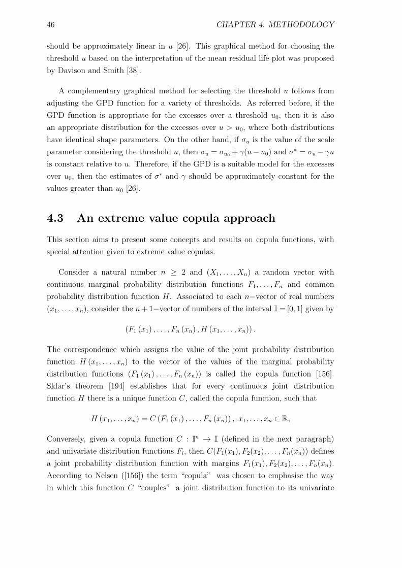
46 CHAPTER 4. METHODOLOGY
should be approximately linear in u [26]. This graphical method for choosing the
threshold u based on the interpretation of the mean residual life plot was proposed
by Davison and Smith [38].
A complementary graphical method for selecting the threshold u follows from
adjusting the GPD function for a variety of thresholds. As referred before, if the
GPD function is appropriate for the excesses over a threshold u0, then it is also
an appropriate distribution for the excesses over u > u0, where both distributions
have identical shape parameters. On the other hand, if σu is the value of the scale
parameter considering the threshold u, then σu = σu0 + γ(u− u0) and σ∗ = σu− γuis constant relative to u. Therefore, if the GPD is a suitable model for the excesses
over u0, then the estimates of σ∗ and γ should be approximately constant for the
values greater than u0 [26].
4.3 An extreme value copula approach
This section aims to present some concepts and results on copula functions, with
special attention given to extreme value copulas.
Consider a natural number n ≥ 2 and (X1, . . . , Xn) a random vector with
continuous marginal probability distribution functions F1, . . . , Fn and common
probability distribution function H. Associated to each n−vector of real numbers
(x1, . . . , xn), consider the n+ 1−vector of numbers of the interval I = [0, 1] given by
(F1 (x1) , . . . , Fn (xn) , H (x1, . . . , xn)) .
The correspondence which assigns the value of the joint probability distribution
function H (x1, . . . , xn) to the vector of the values of the marginal probability
distribution functions (F1 (x1) , . . . , Fn (xn)) is called the copula function [156].
Sklar’s theorem [194] establishes that for every continuous joint distribution
function H there is a unique function C, called the copula function, such that
H (x1, . . . , xn) = C (F1 (x1) , . . . , Fn (xn)) , x1, . . . , xn ∈ R,
Conversely, given a copula function C : In → I (defined in the next paragraph)
and univariate distribution functions Fi, then C(F1(x1), F2(x2), . . . , Fn(xn)) defines
a joint probability distribution function with margins F1(x1), F2(x2), . . . , Fn(xn).
According to Nelsen ([156]) the term “copula” was chosen to emphasise the way
in which this function C “couples” a joint distribution function to its univariate

4.3. AN EXTREME VALUE COPULA APPROACH 47
margins. It should be noted that, by changing the margins, each copula can of
course define infinitely many different joint probability distributions.
A function C : In → I is called a copula when (i) it is such that
C(u) = 0
if at least one coordinate of u = (u1, . . . , un) ∈ In is 0, and
C(u) = ui
if all coordinates of u ∈ In are 1 except ui; and (ii) C is an n-increasing function,
that is given a = (a1, . . . , an) , b = (b1, . . . , bn) ∈ In with ai ≤ bi, i = 1, . . . , n,
2∑i1=1
. . .
2∑in=1
(−1)i1+...+in C (x1i1 , . . . , xnin) ≥ 0,
where xj1 = aj, xj2 = bj. In other words, a copula function is a multivariate
distribution whose univariate margins are all uniform on (0, 1).
Special examples of copula functions are the Frechet–Hoeffding upper bound
copula defined for u = (u1, . . . , un) ∈ In by
Mn(u) = min(u1, . . . , un),
and the product copula defined by
Πn(u) = u1 . . . un.
Because the variables X1, . . . , Xn are independent if and only if the corresponding
copula is Πn [156], this copula is also called the independence copula [182]. The
Frechet–Hoeffding upper bound copula is characterised by the fact that each of the
continuous random variables Xi, i ∈ {1, . . . , n} is almost surely a strictly increasing
function of any of the others if an only if the corresponding copula is Mn [156].
According to Nelsen [155], many of the ways to describe and measure
dependence between random variables remain unchanged under strictly increasing
transformations of these ones. The concordance is one of these scale-invariant
dependence forms. On the other hand, it is also known (cf. e.g. [187]) that the
copula functions capture the properties of dependence between random variables.
In 2002, R. B. Nelsen [155] made a survey about the relationships between
concordance of random variables and their copulas, focusing on the relationship
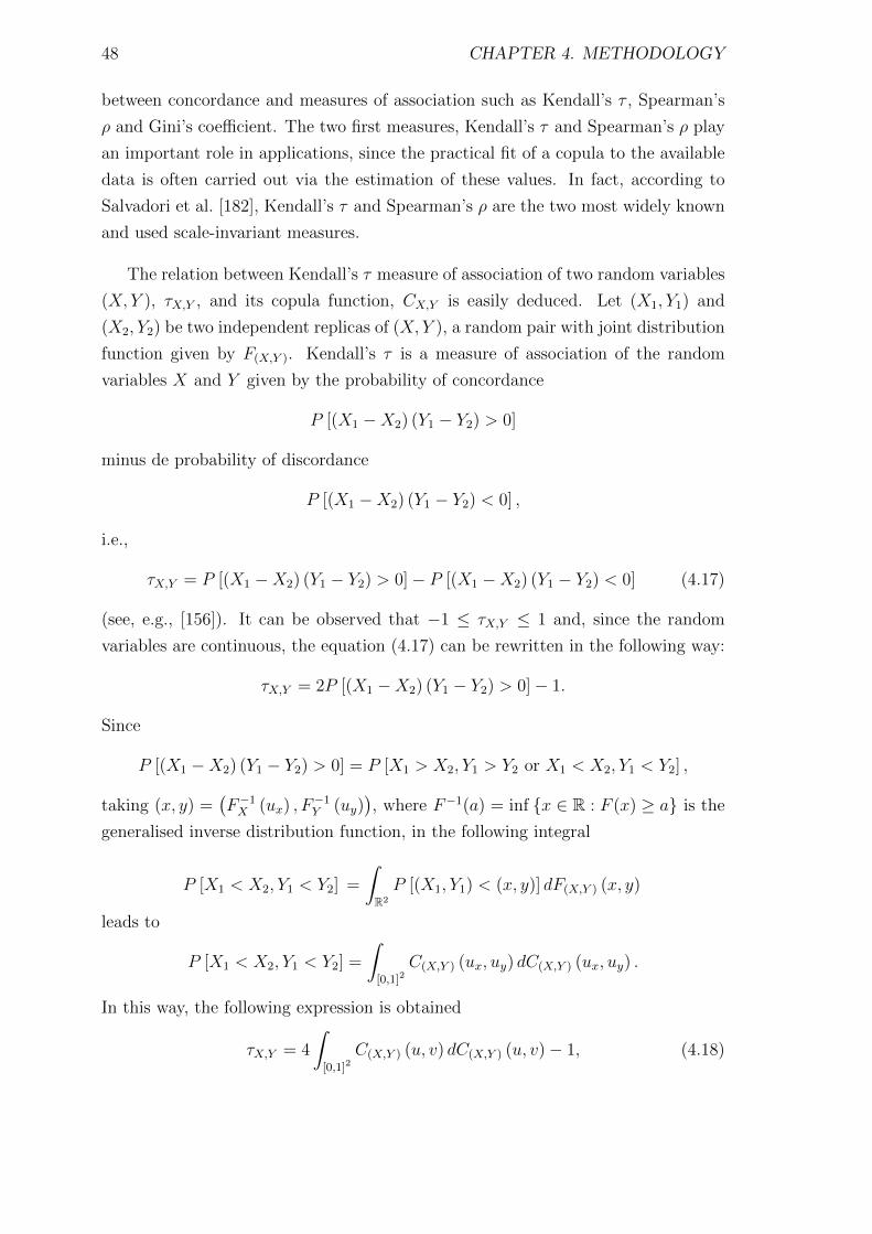
48 CHAPTER 4. METHODOLOGY
between concordance and measures of association such as Kendall’s τ , Spearman’s
ρ and Gini’s coefficient. The two first measures, Kendall’s τ and Spearman’s ρ play
an important role in applications, since the practical fit of a copula to the available
data is often carried out via the estimation of these values. In fact, according to
Salvadori et al. [182], Kendall’s τ and Spearman’s ρ are the two most widely known
and used scale-invariant measures.
The relation between Kendall’s τ measure of association of two random variables
(X, Y ), τX,Y , and its copula function, CX,Y is easily deduced. Let (X1, Y1) and
(X2, Y2) be two independent replicas of (X, Y ), a random pair with joint distribution
function given by F(X,Y ). Kendall’s τ is a measure of association of the random
variables X and Y given by the probability of concordance
P [(X1 −X2) (Y1 − Y2) > 0]
minus de probability of discordance
P [(X1 −X2) (Y1 − Y2) < 0] ,
i.e.,
τX,Y = P [(X1 −X2) (Y1 − Y2) > 0]− P [(X1 −X2) (Y1 − Y2) < 0] (4.17)
(see, e.g., [156]). It can be observed that −1 ≤ τX,Y ≤ 1 and, since the random
variables are continuous, the equation (4.17) can be rewritten in the following way:
τX,Y = 2P [(X1 −X2) (Y1 − Y2) > 0]− 1.
Since
P [(X1 −X2) (Y1 − Y2) > 0] = P [X1 > X2, Y1 > Y2 or X1 < X2, Y1 < Y2] ,
taking (x, y) =(F−1X (ux) , F
−1Y (uy)
), where F−1(a) = inf {x ∈ R : F (x) ≥ a} is the
generalised inverse distribution function, in the following integral
P [X1 < X2, Y1 < Y2] =
∫R2
P [(X1, Y1) < (x, y)] dF(X,Y ) (x, y)
leads to
P [X1 < X2, Y1 < Y2] =
∫[0,1]2
C(X,Y ) (ux, uy) dC(X,Y ) (ux, uy) .
In this way, the following expression is obtained
τX,Y = 4
∫[0,1]2
C(X,Y ) (u, v) dC(X,Y ) (u, v)− 1, (4.18)
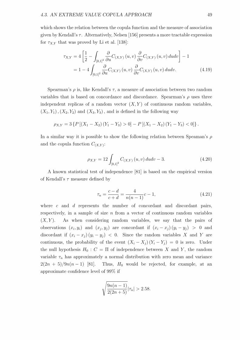
4.3. AN EXTREME VALUE COPULA APPROACH 49
which shows the relation between the copula function and the measure of association
given by Kendall’s τ . Alternatively, Nelsen [156] presents a more tractable expression
for τX,Y that was proved by Li et al. [138]:
τX,Y = 4
[1
2−∫[0,1]2
∂
∂uC(X,Y ) (u, v)
∂
∂vC(X,Y ) (u, v) dudv
]− 1
= 1− 4
∫[0,1]2
∂
∂uC(X,Y ) (u, v)
∂
∂vC(X,Y ) (u, v) dudv. (4.19)
Spearman’s ρ is, like Kendall’s τ, a measure of association between two random
variables that is based on concordance and discordance. Spearman’s ρ uses three
independent replicas of a random vector (X, Y ) of continuous random variables,
(X1, Y1) , (X2, Y2) and (X3, Y3) , and is defined in the following way
ρX,Y = 3 {P [(X1 −X2) (Y1 − Y3) > 0]− P [(X1 −X2) (Y1 − Y3) < 0]} .
In a similar way it is possible to show the following relation between Speaman’s ρ
and the copula function C(X,Y ):
ρX,Y = 12
∫[0,1]2
C(X,Y ) (u, v) dudv − 3. (4.20)
A known statistical test of independence [81] is based on the empirical version
of Kendall’s τ measure defined by
τn =c− dc+ d
=4
n(n− 1)c− 1, (4.21)
where c and d represents the number of concordant and discordant pairs,
respectively, in a sample of size n from a vector of continuous random variables
(X, Y ). As when considering random variables, we say that the pairs of
observations (xi, yi) and (xj, yj) are concordant if (xi − xj) (yi − yj) > 0 and
discordant if (xi − xj) (yi − yj) < 0. Since the random variables X and Y are
continuous, the probability of the event (Xi −Xj) (Yi − Yj) = 0 is zero. Under
the null hypothesis H0 : C = Π of independence between X and Y , the random
variable τn has approximately a normal distribution with zero mean and variance
2(2n + 5)/9n(n− 1) [81]. Thus, H0 would be rejected, for example, at an
approximate confidence level of 99% if√9n(n− 1)
2(2n+ 5)|τn| > 2.58.
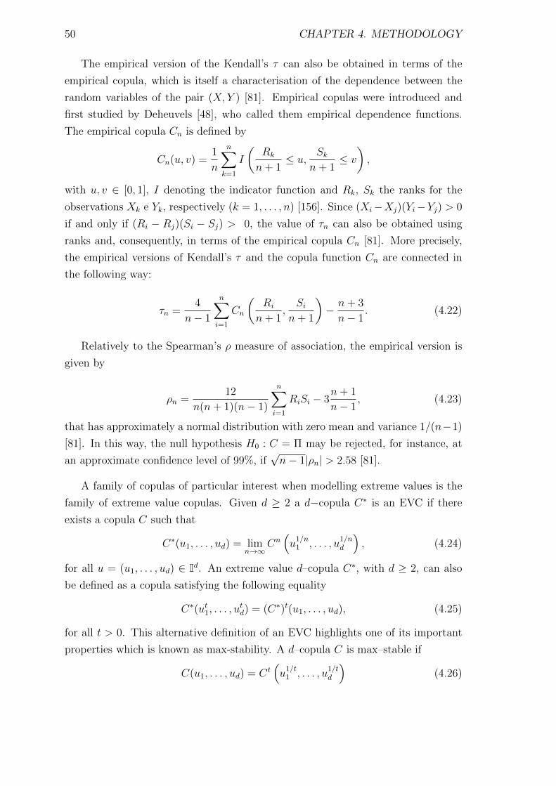
50 CHAPTER 4. METHODOLOGY
The empirical version of the Kendall’s τ can also be obtained in terms of the
empirical copula, which is itself a characterisation of the dependence between the
random variables of the pair (X, Y ) [81]. Empirical copulas were introduced and
first studied by Deheuvels [48], who called them empirical dependence functions.
The empirical copula Cn is defined by
Cn(u, v) =1
n
n∑k=1
I
(Rk
n+ 1≤ u,
Skn+ 1
≤ v
),
with u, v ∈ [0, 1], I denoting the indicator function and Rk, Sk the ranks for the
observations Xk e Yk, respectively (k = 1, . . . , n) [156]. Since (Xi−Xj)(Yi−Yj) > 0
if and only if (Ri − Rj)(Si − Sj) > 0, the value of τn can also be obtained using
ranks and, consequently, in terms of the empirical copula Cn [81]. More precisely,
the empirical versions of Kendall’s τ and the copula function Cn are connected in
the following way:
τn =4
n− 1
n∑i=1
Cn
(Ri
n+ 1,Si
n+ 1
)− n+ 3
n− 1. (4.22)
Relatively to the Spearman’s ρ measure of association, the empirical version is
given by
ρn =12
n(n+ 1)(n− 1)
n∑i=1
RiSi − 3n+ 1
n− 1, (4.23)
that has approximately a normal distribution with zero mean and variance 1/(n−1)
[81]. In this way, the null hypothesis H0 : C = Π may be rejected, for instance, at
an approximate confidence level of 99%, if√n− 1|ρn| > 2.58 [81].
A family of copulas of particular interest when modelling extreme values is the
family of extreme value copulas. Given d ≥ 2 a d−copula C∗ is an EVC if there
exists a copula C such that
C∗(u1, . . . , ud) = limn→∞
Cn(u1/n1 , . . . , u
1/nd
), (4.24)
for all u = (u1, . . . , ud) ∈ Id. An extreme value d–copula C∗, with d ≥ 2, can also
be defined as a copula satisfying the following equality
C∗(ut1, . . . , utd) = (C∗)t(u1, . . . , ud), (4.25)
for all t > 0. This alternative definition of an EVC highlights one of its important
properties which is known as max-stability. A d–copula C is max–stable if
C(u1, . . . , ud) = Ct(u1/t1 , . . . , u
1/td
)(4.26)

4.3. AN EXTREME VALUE COPULA APPROACH 51
is valid for all t > 0 and u ∈ Id.
For example, C = Πd given by Πd(u1, . . . , ud) = u1 . . . ud is a extreme value
d–copula for d ≥ 2. In fact,
Πd(ut1, . . . , u
td) = ut1 . . . u
td = Πt
d(u1, . . . , ud). (4.27)
The Frechet–Hoeffding upper bound copula is also an EVC since
Md(ut1, . . . , u
td) = min
{ut1, . . . , u
td
}= M t
d(u1, . . . , ud). (4.28)
The weighted geometric means of Πd and Md, known as Cuadras–Auge family
of copulas, are also extreme value copulas. For θ ∈ I, the members of the Cuadras–
Auge’s family of copulas are given by
Cθ(u) = Π1−θd (u)M θ
d (u), (4.29)
where u ∈ Id and d ≥ 2. In fact, from (4.27) and (4.28) it follows that
Cθ(ut) = Π1−θ
d
(ut)M θ
d (ut) =[Π1−θd (u)
]t [M θ
d (u)]t
= Ctθ(u) (4.30)
for ut = (ut1, . . . , utd).
More generally, if A and B are d–EVC then
Cα1,...,αd(u) = A (uα11 , . . . , u
αdd )B
(u1−α11 , . . . , u1−αdd
)defines a family of d–EVC with parameters α1, . . . , αd ∈ I. Indeed, from (4.26)
follows that
Ctα1,...,αd
(u1/t1 , . . . , u
1/td ) = At
(uα1/t1 , . . . , u
αd/td
)Bt(u(1−α1)/t1 , . . . , u
(1−αd)/td
)= A (uα1
1 , . . . , uαdd )B
(u1−α11 , . . . , u1−αdd
)= Cα1,...,αd(u1, . . . , ud).
These facts allow the construction of a more versatile family of extreme value
copulas. For example, taking d = 3, the three–dimensional Cuadras–Auge copula
for A, and Π3 for B, defined respectively by
A(u1, u2, u3) = (u1u2u3)1−θ (min (u1, u2, u3))
θ , θ ∈ I,
and
B(u1, u2, u3) = u1u2u3,
52 CHAPTER 4. METHODOLOGY
it follows that
Cα1,α2,α3(u1, u2, u3) = A (uα11 , u
α22 , u
α33 )B
(u1−α11 , u1−α2
2 , u1−α32
)= u
α1(1−θ)1 u
α2(1−θ)2 u
α3(1−θ)3 min
(uθα11 , uθα2
2 , uθα33
)u1−α11 u1−α2
2 u1−α33
= u1−α1θ1 u1−α2θ
2 u1−α3θ3 min
(uθα11 , uθα2
2 , uθα33
)defines a family of 3-EVC. Letting βi = θαi ∈ I this family can be defined in the
following way
C(u1, u2, u3) = Π3i=1u
1−βii min
(uβ11 , u
β22 , u
β33
). (4.31)
The two-dimensional marginals of C, which are obtained when ui → 1, for i = 1, 2
or 3, are Marshall–Olkin bivariate copulas with parameters (βi, βj) for i 6= j, with
i, j = 1, 2, 3. The Marshall–Olkin copula received its name from Ingram Olkin and
Albert Marshall who in 1967 [145] characterised a bivariate distribution, assuming
that it had an exponential marginal and that the following functional equation hold:
F (X,Y ) (s1 + t, s2 + t) = F (X,Y ) (s1, s2)F (X,Y ) (t, t) , (4.32)
where X and Y are two random variables, F (X,Y ) (s, t) = P (X > s, Y > t), with
s1, s2, t > 0.2 Condition (4.32) together with the conditions that make F(X,Y ) a
cumulative distribution function lead to the bivariate exponential distribution of
two random variables with parameters λ1, λ2, λ12 > 0, which can be denoted by
(X, Y ) _ BE (λ1, λ2, λ12) , with joint survival probability function given by
F (X,Y ) (x, y) = P (X > x, Y > y) = exp [−λ1x− λ2y − λ12 max (x, y)] , x, y > 0.
(4.33)
What is known today as the Marshall–Olkin copula (cf. e.g. [182]) should in fact
be known as the Marshall–Olkin survival copula. A survival copula of two random
variables X and Y is the function C(X,Y ) : [0, 1]2 → [0, 1] such that
F (X,Y ) (x, y) = C(X,Y )
(FX (x) , F Y (y)
), (4.34)
2This distribution was derived by Marshall and Olkin as the model to the life of a two–
component system that survives or dies according to the occurrences of “shocks” to each or both
of the components, being the fatal shocks governed by Poisson process {NS (t) , t ≥ 0} that with
rate λS , S ⊆ {1, 2}, destroys the components with indexes in S. Equation (4.32) is a natural
generalisation of the 1–dimensional exponential distribution property given by
FX (s+ t) = FX (s)FX (t) ,
thus representing a particular type of the lack of memory property.

4.3. AN EXTREME VALUE COPULA APPROACH 53
which is related to the copula C of X and Y in the following way:
C(X,Y ) (u, v) = u+ v − 1 + C(X,Y ) (1− u, 1− v) (4.35)
(see, e.g., [156], page 33). From the expression (4.33) it follows that
F (X,Y ) (x, y) =
{exp [− (λ1 + λ12)x− λ2y] , x > y
exp [−λ1x− (λ2 + λ12) y] , x ≤ y
=
FX (x) exp[− λ2λ2+λ12
(λ2 + λ12) y]
, x > y
F Y (y) exp[− λ1λ1+λ12
(λ1 + λ12)x]
, x ≤ y
=
{FX (x)F Y (y)1−β , x > y
F Y (y)FX (x)1−α , x ≤ y,
where α = λ12λ1+λ12
and β = λ12λ2+λ12
. Taking u = FX (x) and v = F Y (y), i.e.,
x = − 1λ1+λ12
lnu and y = − 1λ2+λ12
ln v, and noting that
x > y ⇔ − 1
λ1 + λ12lnu > − 1
λ2 + λ12ln v
⇔ −α lnu > −β ln v ⇔ uα < vβ ⇔ uαβ < v,
the following definition for the bivariate Marshall–Olkin (survival) copula is deduced
for the random pair (X, Y ) _ BE (λ1, λ2, λ12), λ1, λ2, λ12 > 0, for u, v ∈ [0, 1]:
C(X,Y ) (u, v) =
{u1−αv, v ≤ uα/β
uv1−β, v > uα/β(4.36)
= min(u1−αv, uv1−β). (4.37)
Replacing the expression (4.36) in the integral defined in (4.19) it follows that
τX,Y =
∫[0,1]2
∂
∂uC(X,Y ) (u, v)
∂
∂vC(X,Y ) (u, v) dudv
=
∫ 1
0
du
[∫ 1
uα/β
∂
∂uuv1−β
∂
∂vuv1−βdv +
∫ uα/β
0
∂
∂uvu1−α
∂
∂vvu1−αdv
]
=
∫ 1
0
u (1− β)
[v2−2β
2− 2β
]v=1
v=uα/β+ u1−2α (1− α)
[v2
2
]v=uα/βv=0
du
=1
2
∫ 1
0
u− u1−2α+2αβ + u1−2α+2α
β − αu1−2α+2αβ du
=1
2
∫ 1
0
u− αu1−2α+2αβ du =
1
2
[u2
2− α u2−2α+2α
β
2− 2α + 2αβ
]1u=0
=1
4
[1− βα
β − βα + α
],
54 CHAPTER 4. METHODOLOGY
i.e.,
τX,Y =αβ
α− αβ + β, (4.38)
which can be written in the following way
τ = τX,Y =1
1α
+ 1β− 1
. (4.39)
Inverting this relationship, e.g., for α, it follows that
1
τ=
1
α+
1
β− 1⇔ α =
11τ− 1
β+ 1
. (4.40)
A similar relation can be written for the Spearman’s ρ association measure3 but
considering that (see, e.g., [125]) the convergence of τn to normality for increasing
sample size is quicker than that of ρn from now on only Kendall’s τ will be used.
Expressions (4.39) and (4.40) allow the estimation of the parameters β1, β2 and
β3 from the extreme value copula C defined in (4.31), using the estimated values of
Kendall’s τ . Indeed, writing, for simplicity, τi,j instead of τXi,Xj , for i, j ∈ {1, 2, 3},i 6= j, from
1
βi=
1
τ i,j− 1
βj+ 1
3If (X,Y ) is a random pair whose copula function is given by the bivariate Marshall–Olkin
survival copula given by (4.36), then
ρ = ρX,Y =3αβ
2α− αβ + 2β. (4.41)
The association measures Kendall’s τ and Spearman’s ρ for a random pair having as copula the
bivariate Marshall–Olkin survival copula family are given by the expression (4.38) and (4.41).
Replacing α given by expression (4.40), α = 11τ − 1
β +1, in the equality given by (4.41) a relationship
between the measures is obtained:
ρ =3αβ
2α− αβ + 2β=
3β
2− β + 2βα=
3β
2− β + 2βτ −
2ββ + 2β
=3
2τ + 1
=3τ
2 + τ,
i.e.,
ρ =3τ
2 + τ,
for ρ and τ both in [0, 1] .

4.3. AN EXTREME VALUE COPULA APPROACH 55
it follows that, for k ∈ {1, 2, 3}\{i, j},
1
βi=
1
τ i,j− 1
βj+ 1 =
1
τ i,j− (
1
τ j,k− 1
βk+ 1) + 1
=1
τ i,j− 1
τ j,k+
1
βk=
1
τ i,j− 1
τ j,k+ (
1
τ i,k− 1
βi+ 1)
= 1 +1
τ i,j+
1
τ i,k− 1
τ j,k− 1
βi
that is equivalent to2
βi= 1 +
1
τ i,j+
1
τ i,k− 1
τ j,k.
Therefore,
1
βi=
1
2
(1 +
1
τ i,j+
1
τ i,k− 1
τ j,k
), (4.42)
where (i, j, k) is a permutation of (1, 2, 3).
These relationships allow the estimation of the probability of extremal events.
In practice, given a random vector (X1, . . . , Xn), an event is defined as extreme if
one or more variables exceed some given high values. Of particular practical interest
is the event
Ex1,...,xnn = {X1 > x1, ..., Xn > xn} .
Taking n = 3, assuming that the random vector (X1, X2, X3) has as continuous
distribution with copula function C and taking ui = P (Xi ≤ xi), it follows that
P (Ex1,x2,x33 ) = P (X1 > x1, X2 > x2, X3 > x3)
= 1−3∑i=1
P (Xi ≤ xi) +3∑
i,j=1i<j
P (Xi ≤ xi, Xj ≤ xj)
−P (X1 ≤ x1, X2 ≤ x2, X3 ≤ x3)
= 1− u1 − u2 − u3 − C (u1, u2, u3) + C (u1, u2, 1)
+ C (u1, 1, u3) + C (1, u2, u3) . (4.43)
Let Xi denote the observation at the i–th rain gauge station and xi,q the (1−q)–quantile of Xi for q ∈ (0, 1) and i ∈ {1, 2, 3}, and consider the extremal event
Eq = Ex1,q ,x2,q ,x3,q3 = {X1 > x1,q, X2 > x2,q, X3 > x3,q} .
56 CHAPTER 4. METHODOLOGY
The return period rq of Eq is given by 1pq
, with pq = P (Eq), which is given by
pq = P(Ex1,q ,x2,q ,x3,q3
)= 1− 3q − C (q, q, q) + C (q, q, 1) + C (q, 1, q) + C (1, q, q) . (4.44)
In this section, the concepts and methodologies necessary to the application of
the chosen extreme copula approach were presented and discussed. Kendall’s τ
association measure and the extreme value copulas involving the Marshall–Olkin
family will have a major role in such application, whose results and discussion are
presented in Section 5.3.
Chapter 5
Results and discussion
5.1 Annual maxima – Gumbel’s model approach
It was Emil Gumbel who in 1958 [107] firstly proposed the block maxima approach
in the study of statistics of extremes. Under this approach, also called block maxima
model, a sample of size m is divided into n sub–samples of size r. Then, the sample of
the maxima of these n sub-samples is fitted by one of the extremal models (Gumbel,
Frechet or Weibull) [88]. Usually, when data results from a record of some quantity
along time, the subsamples coincide with the records of the years and n is the number
of years sampled. This is why sometimes this model is also referred as the annual
maxima approach. Among the extremal models, Gumbel distribution is a commonly
used model for hydrological extremes, especially when quantifying risk associated
with extreme rainfall [129]. However, there are studies suggesting that the Gumbel
distribution may underestimate the largest extreme rainfall amounts [132, 129, 223,
e.g.]. To overcome this problem, statistical practioners tend to prefer to fit the
GEV distribution to the data [26, 132, 129, e.g.]. According to Hosking et al. [119],
the GEV distribution has been widely utilised for modelling extremes of natural
phenomena since this use was recommended in a report of the Natural Environment
Research Council [157]. In this report, GEV distributions were fitted to 32 samples,
with dimension sizes of at least 30, by the application of the ML estimation method.
The major disadvantage of this method is that it can be extremely erratic for small
samples as mentioned by Katz et al. [124]. The good performance of the PWM
method for small samples [119] was a factor that made this method more popular
than ML in applications to hydrological extremes. The differences between these
two methods have been analysed and some improvements have been proposed by
a number of authors [28, 53, e.g.]. In this section, these two methods, ML and
57

58 CHAPTER 5. RESULTS AND DISCUSSION
PWM, were used to obtain estimates for the GEV distribution parameters. Also,
tests based on the likelihood ratio statistic and on the PWM were used to test the
hypothesis of a Gumbel distribution versus a GEV distribution. The 50– and 100–
year return level estimates were obtained and, in addition, the existence of trends
in the parameters’ values was also analysed.
5.1.1 Dataset I
The dataset analysed in this subsection consists of annual maximum precipitation
data from seven rain gauge stations in Madeira Island maintained by IPMA whose
locations are shown in Figure 5.1. Table 5.1 provides information about each
data sample, namely size (n), measurement period and the corresponding station’s
altitude, identification name and letter.
Figure 5.1: Location and altitude range of the rain gauge stations–Dataset I (Map
data c©2014 Google).
Table 5.1: Dataset I: annual maximum precipitation (source: IPMA).
Station Altitude (m) Period n
Areeiro (A) 1610 1961–1992 31
Bica da Cana (B) 1560 1961–2008 40
Santo da Serra (I) 660 1970–2009 38
Santana (P) 380 1942–2007 59
Funchal (U) 58 1949–2009 61
Santa Catarina (V) 49 1961–2009 48
Lugar de Baixo (X) 15 1961–2004 43

5.1. ANNUAL MAXIMA – GUMBEL’S MODEL APPROACH 59
Hydrological time records may not satisfy the basic requirements of extreme
value theory as they can often be autocorrelated and not identically distributed
[62]. However, according to Leadbetter and Rootzen [136], under weak dependence
restrictions, the general “type” of limiting distribution for the maximum is the same
as for an independent and identically distributed sequence. The non-stationarity can
be accounted, for example, by subdividing the dataset into blocks that are considered
to be homogeneous or by letting the parameters in the GEV distribution depend on
time [62]. So, although the full set provided by IPMA contains a series of values
for each year, only the annual maxima are considered here. Thus, in this way,
intra-year dependencies are avoided and the supposition that the data x1, ..., xn are
realisations from a sequence X1, ..., Xn of independent and identically distributed
random variables, all with common extreme value distribution may be considered
as a valid assumption [61]. Nevertheless, a procedure to detect non-stationarities
considered in the work of Koutsoyiannis and Baloutsos [132] was applied to the
dataset of each of the seven locations. The procedure consists in dividing each station
data record into to four subsets with approximately the same length record and then
test the hypothesis that all four subseries have identical distributions by the non
parametric Kruskal-Wallis test. The four subsamples record length (n1, n2, n3, n4),
the Kruskal-Wallis statistic test value and the corresponding p–value for each station
dataset, obtained by the application of function kruskal.test in the stats R language
package [178], are displayed in Table 5.2.
Table 5.2: Records length, Kruskal-Wallis statistic test value and p–value–Dataset I.
Station (n1, n2, n3, n4) Statistic test value p–value
Areeiro (A) (8, 8, 8, 7) 6.0318 0.1101
Bica da Cana (B) (10, 10, 10, 10) 0.7098 0.8709
Santo da Serra (I) (10, 10, 10, 8) 5.5432 0.1361
Santana (P) (15, 15, 15, 14) 2.1671 0.5385
Funchal (U) (16, 16, 16, 13) 2.0754 0.5569
Santa Catarina (V) (12, 12, 12, 12) 0.5341 0.9113
Lugar de Baixo (X) (11, 11, 11, 10) 1.6237 0.6540
At a 0.05 significance level, the hypothesis of homogeneity is not rejected
for all seven station datasets. As mentioned above, another way to deal with
non-stationarities is to let the parameters in the chosen distribution to be time–
dependent. So, besides testing the null hypothesis H0 of a Gumbel distribution
(Model 2) against the alternative hypothesis H1 of another extreme value
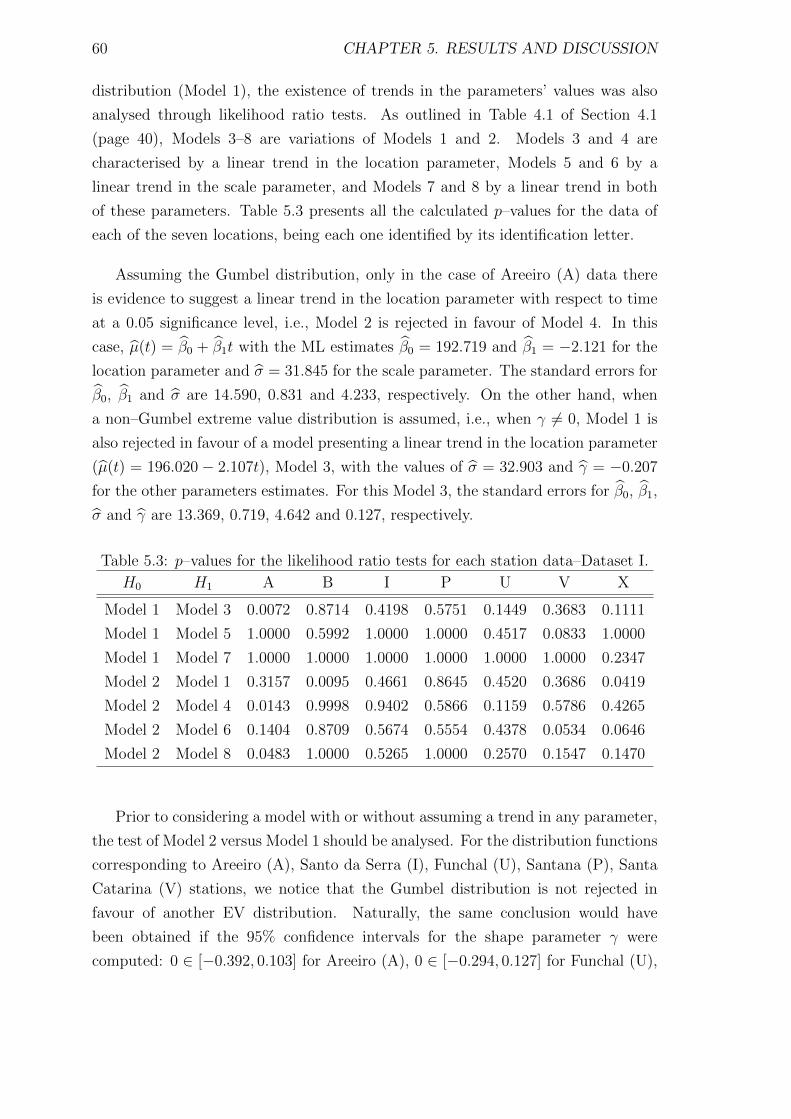
60 CHAPTER 5. RESULTS AND DISCUSSION
distribution (Model 1), the existence of trends in the parameters’ values was also
analysed through likelihood ratio tests. As outlined in Table 4.1 of Section 4.1
(page 40), Models 3–8 are variations of Models 1 and 2. Models 3 and 4 are
characterised by a linear trend in the location parameter, Models 5 and 6 by a
linear trend in the scale parameter, and Models 7 and 8 by a linear trend in both
of these parameters. Table 5.3 presents all the calculated p–values for the data of
each of the seven locations, being each one identified by its identification letter.
Assuming the Gumbel distribution, only in the case of Areeiro (A) data there
is evidence to suggest a linear trend in the location parameter with respect to time
at a 0.05 significance level, i.e., Model 2 is rejected in favour of Model 4. In this
case, µ(t) = β0 + β1t with the ML estimates β0 = 192.719 and β1 = −2.121 for the
location parameter and σ = 31.845 for the scale parameter. The standard errors for
β0, β1 and σ are 14.590, 0.831 and 4.233, respectively. On the other hand, when
a non–Gumbel extreme value distribution is assumed, i.e., when γ 6= 0, Model 1 is
also rejected in favour of a model presenting a linear trend in the location parameter
(µ(t) = 196.020 − 2.107t), Model 3, with the values of σ = 32.903 and γ = −0.207
for the other parameters estimates. For this Model 3, the standard errors for β0, β1,
σ and γ are 13.369, 0.719, 4.642 and 0.127, respectively.
Table 5.3: p–values for the likelihood ratio tests for each station data–Dataset I.
H0 H1 A B I P U V X
Model 1 Model 3 0.0072 0.8714 0.4198 0.5751 0.1449 0.3683 0.1111
Model 1 Model 5 1.0000 0.5992 1.0000 1.0000 0.4517 0.0833 1.0000
Model 1 Model 7 1.0000 1.0000 1.0000 1.0000 1.0000 1.0000 0.2347
Model 2 Model 1 0.3157 0.0095 0.4661 0.8645 0.4520 0.3686 0.0419
Model 2 Model 4 0.0143 0.9998 0.9402 0.5866 0.1159 0.5786 0.4265
Model 2 Model 6 0.1404 0.8709 0.5674 0.5554 0.4378 0.0534 0.0646
Model 2 Model 8 0.0483 1.0000 0.5265 1.0000 0.2570 0.1547 0.1470
Prior to considering a model with or without assuming a trend in any parameter,
the test of Model 2 versus Model 1 should be analysed. For the distribution functions
corresponding to Areeiro (A), Santo da Serra (I), Funchal (U), Santana (P), Santa
Catarina (V) stations, we notice that the Gumbel distribution is not rejected in
favour of another EV distribution. Naturally, the same conclusion would have
been obtained if the 95% confidence intervals for the shape parameter γ were
computed: 0 ∈ [−0.392, 0.103] for Areeiro (A), 0 ∈ [−0.294, 0.127] for Funchal (U),
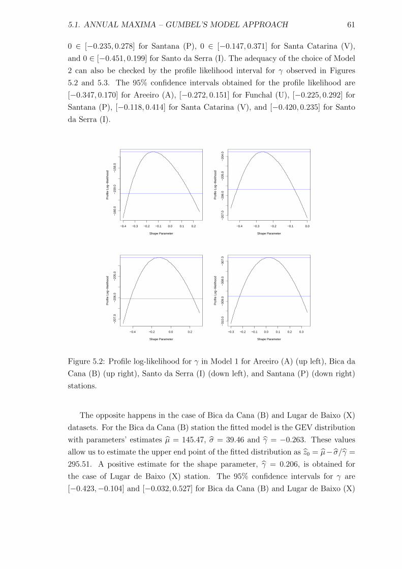
5.1. ANNUAL MAXIMA – GUMBEL’S MODEL APPROACH 61
0 ∈ [−0.235, 0.278] for Santana (P), 0 ∈ [−0.147, 0.371] for Santa Catarina (V),
and 0 ∈ [−0.451, 0.199] for Santo da Serra (I). The adequacy of the choice of Model
2 can also be checked by the profile likelihood interval for γ observed in Figures
5.2 and 5.3. The 95% confidence intervals obtained for the profile likelihood are
[−0.347, 0.170] for Areeiro (A), [−0.272, 0.151] for Funchal (U), [−0.225, 0.292] for
Santana (P), [−0.118, 0.414] for Santa Catarina (V), and [−0.420, 0.235] for Santo
da Serra (I).
−0.4 −0.3 −0.2 −0.1 0.0 0.1 0.2
−16
0.0
−15
9.0
−15
8.0
Shape Parameter
Pro
file
Log−
likel
ihoo
d
−0.4 −0.3 −0.2 −0.1 0.0
−20
7.0
−20
6.0
−20
5.0
−20
4.0
Shape Parameter
Pro
file
Log−
likel
ihoo
d
−0.4 −0.2 0.0 0.2
−20
7.0
−20
6.0
−20
5.0
Shape Parameter
Pro
file
Log−
likel
ihoo
d
−0.3 −0.2 −0.1 0.0 0.1 0.2 0.3
−31
0.0
−30
9.0
−30
8.0
−30
7.0
Shape Parameter
Pro
file
Log−
likel
ihoo
d
Figure 5.2: Profile log-likelihood for γ in Model 1 for Areeiro (A) (up left), Bica da
Cana (B) (up right), Santo da Serra (I) (down left), and Santana (P) (down right)
stations.
The opposite happens in the case of Bica da Cana (B) and Lugar de Baixo (X)
datasets. For the Bica da Cana (B) station the fitted model is the GEV distribution
with parameters’ estimates µ = 145.47, σ = 39.46 and γ = −0.263. These values
allow us to estimate the upper end point of the fitted distribution as z0 = µ− σ/γ =
295.51. A positive estimate for the shape parameter, γ = 0.206, is obtained for
the case of Lugar de Baixo (X) station. The 95% confidence intervals for γ are
[−0.423,−0.104] and [−0.032, 0.527] for Bica da Cana (B) and Lugar de Baixo (X)
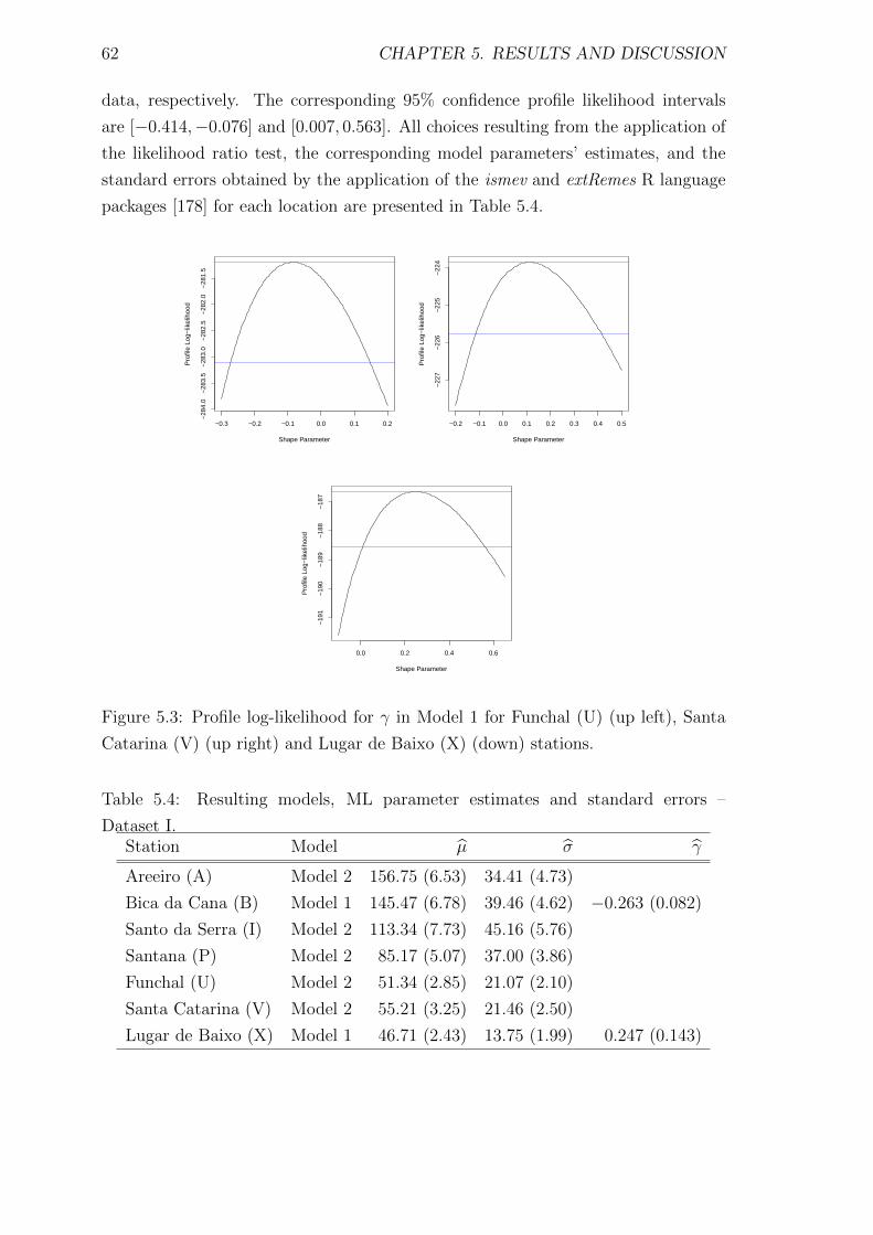
62 CHAPTER 5. RESULTS AND DISCUSSION
data, respectively. The corresponding 95% confidence profile likelihood intervals
are [−0.414,−0.076] and [0.007, 0.563]. All choices resulting from the application of
the likelihood ratio test, the corresponding model parameters’ estimates, and the
standard errors obtained by the application of the ismev and extRemes R language
packages [178] for each location are presented in Table 5.4.
−0.3 −0.2 −0.1 0.0 0.1 0.2
−28
4.0
−28
3.5
−28
3.0
−28
2.5
−28
2.0
−28
1.5
Shape Parameter
Pro
file
Log−
likel
ihoo
d
−0.2 −0.1 0.0 0.1 0.2 0.3 0.4 0.5
−22
7−
226
−22
5−
224
Shape Parameter
Pro
file
Log−
likel
ihoo
d
0.0 0.2 0.4 0.6
−19
1−
190
−18
9−
188
−18
7
Shape Parameter
Pro
file
Log−
likel
ihoo
d
Figure 5.3: Profile log-likelihood for γ in Model 1 for Funchal (U) (up left), Santa
Catarina (V) (up right) and Lugar de Baixo (X) (down) stations.
Table 5.4: Resulting models, ML parameter estimates and standard errors –
Dataset I.Station Model µ σ γ
Areeiro (A) Model 2 156.75 (6.53) 34.41 (4.73)
Bica da Cana (B) Model 1 145.47 (6.78) 39.46 (4.62) −0.263 (0.082)
Santo da Serra (I) Model 2 113.34 (7.73) 45.16 (5.76)
Santana (P) Model 2 85.17 (5.07) 37.00 (3.86)
Funchal (U) Model 2 51.34 (2.85) 21.07 (2.10)
Santa Catarina (V) Model 2 55.21 (3.25) 21.46 (2.50)
Lugar de Baixo (X) Model 1 46.71 (2.43) 13.75 (1.99) 0.247 (0.143)

5.1. ANNUAL MAXIMA – GUMBEL’S MODEL APPROACH 63
The adequacy of the model was tested through the Kolmogorov-Smirnov test by
the application of the function gofstat in the fitdistrplus R language package [178].
The test statistic values obtained when Model 2 was tested were 0.1146 for Areeiro
(A), 0.0602 for Funchal (U), 0.0955 for Santana (P), 0.0948 Santa Catarina (V),
and 0.0953 for Santo da Serra (I). In the two cases where Model 1 was tested, the
calculated test statistic values were 0.0708 and 0.0669 for Bica da Cana (B) and
Lugar de Baixo (X), respectively. So, each station data do not provide sufficient
evidence to conclude that the chosen model is not an appropriate model for modelling
the respective annual maxima.
The same models’ choices are made when the hypothesis of a Gumbel distribution
is analysed by a test based on the PWM estimate of γ presented by Hosking et
al. [118]. The value for the test statistic given by (4.7), Z = γ(n/0.5633)1/2, is not
significant in comparison with the critical values of the standard normal distribution
for Areeiro (A), Funchal (U), Santana (P), Santa Catarina (V) and Santo da Serra
(I) data. As before, the opposite happens with the cases of Bica da Cana (B) and
Lugar de Baixo (X). The models’ choices resulting from the application of this test
are presented in Table 5.5, which also shows the corresponding model parameter
estimates obtained by the use of the fExtremes R package.
Table 5.5: Resulting models and PWM parameter estimates–Dataset I.
Station Model µ σ γ
Areeiro (A) Model 2 93.04 143.22
Bica da Cana (B) Model 1 145.54 39.52 −0.274
Santo da Serra (I) Model 2 68.10 122.86
Santana (P) Model 2 51.33 96.42
Funchal (U) Model 2 30.92 56.07
Santa Catarina (V) Model 2 33.13 60.78
Lugar de Baixo (X) Model 1 46.74 14.38 0.206
Although for the distributions corresponding to Areeiro (A), Funchal (U),
Santana (P), Santa Catarina (V) and Santo da Serra (I) data there is no significant
evidence to decide to choose a non-Gumbel EV model in opposition to the Gumbel
model, it is observed that the ML estimate for each γ is not zero (see Table 5.6).
The same observation can be made when the PWM estimates are considered.
Besides the γ estimates, Table 5.6 presents the ML and PWM estimates for the
location and scale parameters. The values of estimates are similar for both methods
for Model 1 but that is not the case when the Model 2 is chosen. For the Gumbel
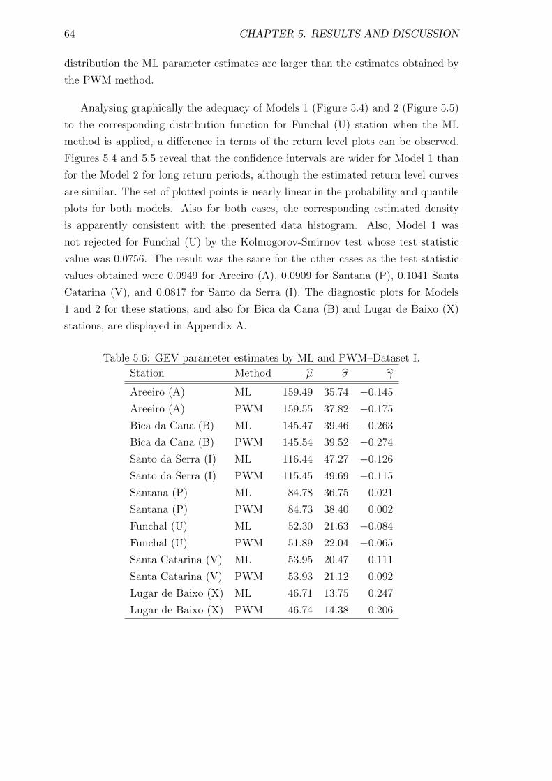
64 CHAPTER 5. RESULTS AND DISCUSSION
distribution the ML parameter estimates are larger than the estimates obtained by
the PWM method.
Analysing graphically the adequacy of Models 1 (Figure 5.4) and 2 (Figure 5.5)
to the corresponding distribution function for Funchal (U) station when the ML
method is applied, a difference in terms of the return level plots can be observed.
Figures 5.4 and 5.5 reveal that the confidence intervals are wider for Model 1 than
for the Model 2 for long return periods, although the estimated return level curves
are similar. The set of plotted points is nearly linear in the probability and quantile
plots for both models. Also for both cases, the corresponding estimated density
is apparently consistent with the presented data histogram. Also, Model 1 was
not rejected for Funchal (U) by the Kolmogorov-Smirnov test whose test statistic
value was 0.0756. The result was the same for the other cases as the test statistic
values obtained were 0.0949 for Areeiro (A), 0.0909 for Santana (P), 0.1041 Santa
Catarina (V), and 0.0817 for Santo da Serra (I). The diagnostic plots for Models
1 and 2 for these stations, and also for Bica da Cana (B) and Lugar de Baixo (X)
stations, are displayed in Appendix A.
Table 5.6: GEV parameter estimates by ML and PWM–Dataset I.
Station Method µ σ γ
Areeiro (A) ML 159.49 35.74 −0.145
Areeiro (A) PWM 159.55 37.82 −0.175
Bica da Cana (B) ML 145.47 39.46 −0.263
Bica da Cana (B) PWM 145.54 39.52 −0.274
Santo da Serra (I) ML 116.44 47.27 −0.126
Santo da Serra (I) PWM 115.45 49.69 −0.115
Santana (P) ML 84.78 36.75 0.021
Santana (P) PWM 84.73 38.40 0.002
Funchal (U) ML 52.30 21.63 −0.084
Funchal (U) PWM 51.89 22.04 −0.065
Santa Catarina (V) ML 53.95 20.47 0.111
Santa Catarina (V) PWM 53.93 21.12 0.092
Lugar de Baixo (X) ML 46.71 13.75 0.247
Lugar de Baixo (X) PWM 46.74 14.38 0.206
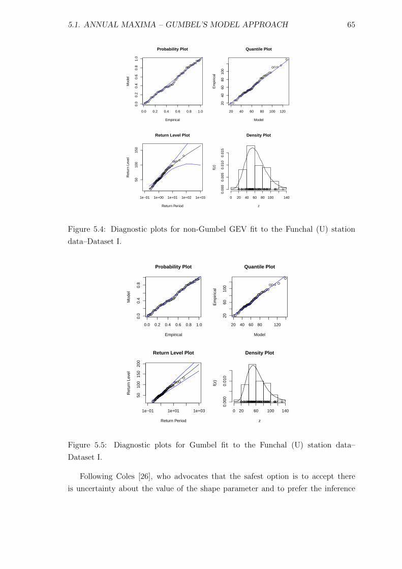
5.1. ANNUAL MAXIMA – GUMBEL’S MODEL APPROACH 65
0.0 0.2 0.4 0.6 0.8 1.0
0.0
0.2
0.4
0.6
0.8
1.0
Probability Plot
Empirical
Mod
el
20 40 60 80 100 120
2040
6080
100
Quantile Plot
Model
Em
piric
al
1e−01 1e+00 1e+01 1e+02 1e+03
5010
015
0
Return Period
Ret
urn
Leve
l
Return Level Plot Density Plot
z
f(z)
0 20 40 60 80 100 140
0.00
00.
005
0.01
00.
015
Figure 5.4: Diagnostic plots for non-Gumbel GEV fit to the Funchal (U) station
data–Dataset I.
0.0 0.2 0.4 0.6 0.8 1.0
0.0
0.4
0.8
Probability Plot
Empirical
Mod
el
20 40 60 80 120
2060
100
Quantile Plot
Model
Em
piric
al
1e−01 1e+01 1e+03
5010
015
020
0
Return Period
Ret
urn
Leve
l
Return Level Plot Density Plot
z
f(z)
0 20 60 100 140
0.00
00.
010
Figure 5.5: Diagnostic plots for Gumbel fit to the Funchal (U) station data–
Dataset I.
Following Coles [26], who advocates that the safest option is to accept there
is uncertainty about the value of the shape parameter and to prefer the inference
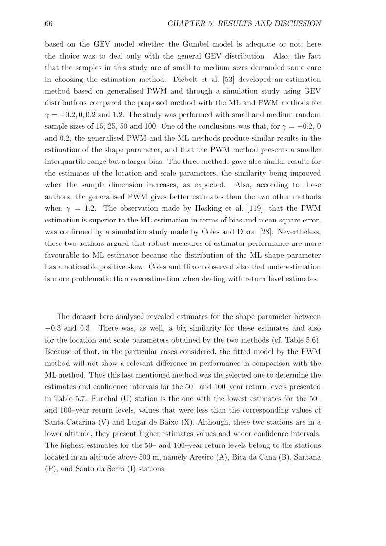
66 CHAPTER 5. RESULTS AND DISCUSSION
based on the GEV model whether the Gumbel model is adequate or not, here
the choice was to deal only with the general GEV distribution. Also, the fact
that the samples in this study are of small to medium sizes demanded some care
in choosing the estimation method. Diebolt et al. [53] developed an estimation
method based on generalised PWM and through a simulation study using GEV
distributions compared the proposed method with the ML and PWM methods for
γ = −0.2, 0, 0.2 and 1.2. The study was performed with small and medium random
sample sizes of 15, 25, 50 and 100. One of the conclusions was that, for γ = −0.2, 0
and 0.2, the generalised PWM and the ML methods produce similar results in the
estimation of the shape parameter, and that the PWM method presents a smaller
interquartile range but a larger bias. The three methods gave also similar results for
the estimates of the location and scale parameters, the similarity being improved
when the sample dimension increases, as expected. Also, according to these
authors, the generalised PWM gives better estimates than the two other methods
when γ = 1.2. The observation made by Hosking et al. [119], that the PWM
estimation is superior to the ML estimation in terms of bias and mean-square error,
was confirmed by a simulation study made by Coles and Dixon [28]. Nevertheless,
these two authors argued that robust measures of estimator performance are more
favourable to ML estimator because the distribution of the ML shape parameter
has a noticeable positive skew. Coles and Dixon observed also that underestimation
is more problematic than overestimation when dealing with return level estimates.
The dataset here analysed revealed estimates for the shape parameter between
−0.3 and 0.3. There was, as well, a big similarity for these estimates and also
for the location and scale parameters obtained by the two methods (cf. Table 5.6).
Because of that, in the particular cases considered, the fitted model by the PWM
method will not show a relevant difference in performance in comparison with the
ML method. Thus this last mentioned method was the selected one to determine the
estimates and confidence intervals for the 50– and 100–year return levels presented
in Table 5.7. Funchal (U) station is the one with the lowest estimates for the 50–
and 100–year return levels, values that were less than the corresponding values of
Santa Catarina (V) and Lugar de Baixo (X). Although, these two stations are in a
lower altitude, they present higher estimates values and wider confidence intervals.
The highest estimates for the 50– and 100–year return levels belong to the stations
located in an altitude above 500 m, namely Areeiro (A), Bica da Cana (B), Santana
(P), and Santo da Serra (I) stations.
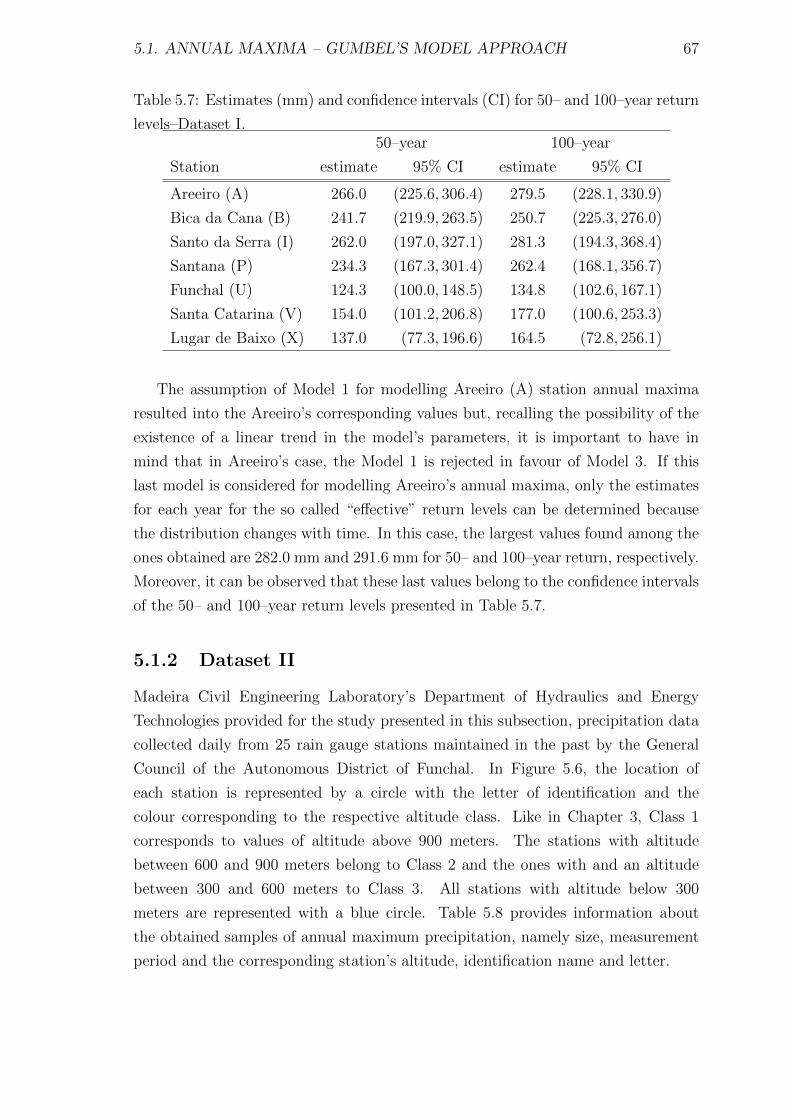
5.1. ANNUAL MAXIMA – GUMBEL’S MODEL APPROACH 67
Table 5.7: Estimates (mm) and confidence intervals (CI) for 50– and 100–year return
levels–Dataset I.50–year 100–year
Station estimate 95% CI estimate 95% CI
Areeiro (A) 266.0 (225.6, 306.4) 279.5 (228.1, 330.9)
Bica da Cana (B) 241.7 (219.9, 263.5) 250.7 (225.3, 276.0)
Santo da Serra (I) 262.0 (197.0, 327.1) 281.3 (194.3, 368.4)
Santana (P) 234.3 (167.3, 301.4) 262.4 (168.1, 356.7)
Funchal (U) 124.3 (100.0, 148.5) 134.8 (102.6, 167.1)
Santa Catarina (V) 154.0 (101.2, 206.8) 177.0 (100.6, 253.3)
Lugar de Baixo (X) 137.0 (77.3, 196.6) 164.5 (72.8, 256.1)
The assumption of Model 1 for modelling Areeiro (A) station annual maxima
resulted into the Areeiro’s corresponding values but, recalling the possibility of the
existence of a linear trend in the model’s parameters, it is important to have in
mind that in Areeiro’s case, the Model 1 is rejected in favour of Model 3. If this
last model is considered for modelling Areeiro’s annual maxima, only the estimates
for each year for the so called “effective” return levels can be determined because
the distribution changes with time. In this case, the largest values found among the
ones obtained are 282.0 mm and 291.6 mm for 50– and 100–year return, respectively.
Moreover, it can be observed that these last values belong to the confidence intervals
of the 50– and 100–year return levels presented in Table 5.7.
5.1.2 Dataset II
Madeira Civil Engineering Laboratory’s Department of Hydraulics and Energy
Technologies provided for the study presented in this subsection, precipitation data
collected daily from 25 rain gauge stations maintained in the past by the General
Council of the Autonomous District of Funchal. In Figure 5.6, the location of
each station is represented by a circle with the letter of identification and the
colour corresponding to the respective altitude class. Like in Chapter 3, Class 1
corresponds to values of altitude above 900 meters. The stations with altitude
between 600 and 900 meters belong to Class 2 and the ones with and an altitude
between 300 and 600 meters to Class 3. All stations with altitude below 300
meters are represented with a blue circle. Table 5.8 provides information about
the obtained samples of annual maximum precipitation, namely size, measurement
period and the corresponding station’s altitude, identification name and letter.
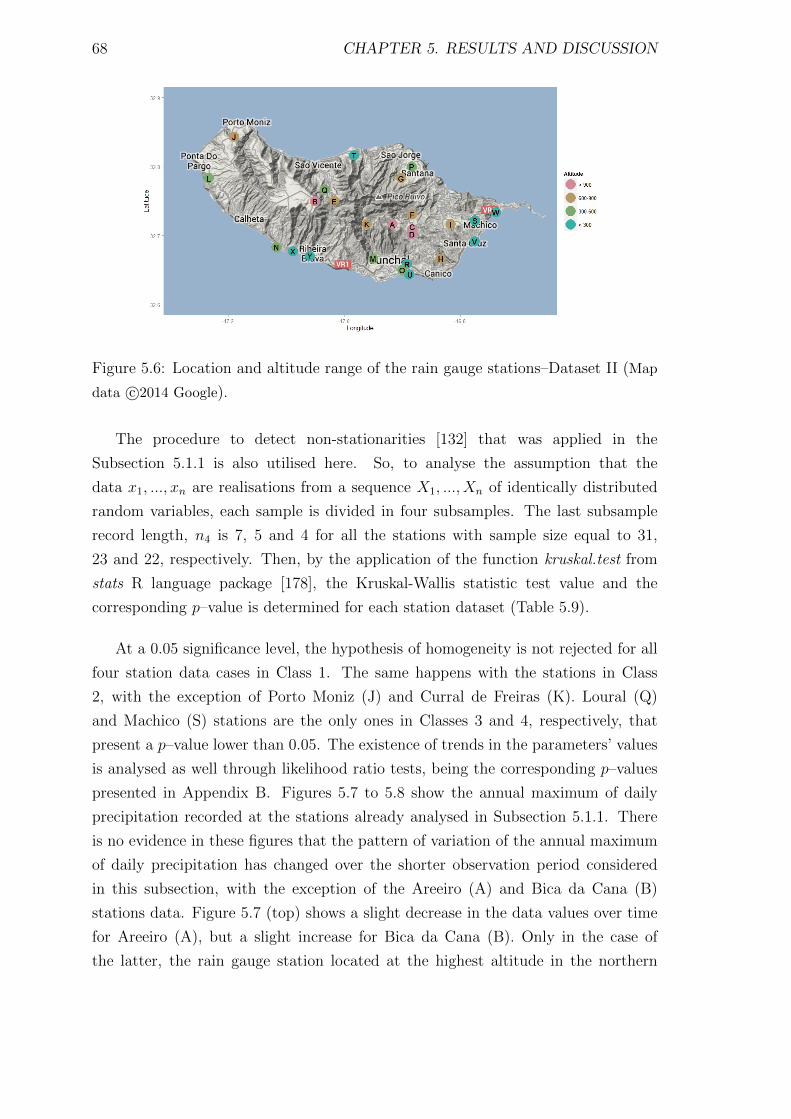
68 CHAPTER 5. RESULTS AND DISCUSSION
Figure 5.6: Location and altitude range of the rain gauge stations–Dataset II (Map
data c©2014 Google).
The procedure to detect non-stationarities [132] that was applied in the
Subsection 5.1.1 is also utilised here. So, to analyse the assumption that the
data x1, ..., xn are realisations from a sequence X1, ..., Xn of identically distributed
random variables, each sample is divided in four subsamples. The last subsample
record length, n4 is 7, 5 and 4 for all the stations with sample size equal to 31,
23 and 22, respectively. Then, by the application of the function kruskal.test from
stats R language package [178], the Kruskal-Wallis statistic test value and the
corresponding p–value is determined for each station dataset (Table 5.9).
At a 0.05 significance level, the hypothesis of homogeneity is not rejected for all
four station data cases in Class 1. The same happens with the stations in Class
2, with the exception of Porto Moniz (J) and Curral de Freiras (K). Loural (Q)
and Machico (S) stations are the only ones in Classes 3 and 4, respectively, that
present a p–value lower than 0.05. The existence of trends in the parameters’ values
is analysed as well through likelihood ratio tests, being the corresponding p–values
presented in Appendix B. Figures 5.7 to 5.8 show the annual maximum of daily
precipitation recorded at the stations already analysed in Subsection 5.1.1. There
is no evidence in these figures that the pattern of variation of the annual maximum
of daily precipitation has changed over the shorter observation period considered
in this subsection, with the exception of the Areeiro (A) and Bica da Cana (B)
stations data. Figure 5.7 (top) shows a slight decrease in the data values over time
for Areeiro (A), but a slight increase for Bica da Cana (B). Only in the case of
the latter, the rain gauge station located at the highest altitude in the northern
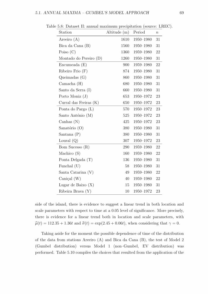
5.1. ANNUAL MAXIMA – GUMBEL’S MODEL APPROACH 69
Table 5.8: Dataset II: annual maximum precipitation (source: LREC).
Station Altitude (m) Period n
Areeiro (A) 1610 1950–1980 31
Bica da Cana (B) 1560 1950–1980 31
Poiso (C) 1360 1959–1980 22
Montado do Pereiro (D) 1260 1950–1980 31
Encumeada (E) 900 1959–1980 22
Ribeiro Frio (F) 874 1950–1980 31
Queimadas (G) 860 1950–1980 31
Camacha (H) 680 1950–1980 31
Santo da Serra (I) 660 1950–1980 31
Porto Moniz (J) 653 1950–1972 23
Curral das Freiras (K) 650 1950–1972 23
Ponta do Pargo (L) 570 1950–1972 23
Santo Antonio (M) 525 1950–1972 23
Canhas (N) 425 1950–1972 23
Sanatorio (O) 380 1950–1980 31
Santana (P) 380 1950–1980 31
Loural (Q) 307 1950–1972 23
Bom Sucesso (R) 290 1959–1980 22
Machico (S) 160 1959–1980 22
Ponta Delgada (T) 136 1950–1980 31
Funchal (U) 58 1950–1980 31
Santa Catarina (V) 49 1959–1980 22
Canical (W) 40 1959–1980 22
Lugar de Baixo (X) 15 1950–1980 31
Ribeira Brava (Y) 10 1950–1972 23
side of the island, there is evidence to suggest a linear trend in both location and
scale parameters with respect to time at a 0.05 level of significance. More precisely,
there is evidence for a linear trend both in location and scale parameters, with
µ(t) = 112.35 + 1.36t and σ(t) = exp(2.45 + 0.06t), when considering that γ = 0.
Taking aside for the moment the possible dependence of time of the distribution
of the data from stations Areeiro (A) and Bica da Cana (B), the test of Model 2
(Gumbel distribution) versus Model 1 (non–Gumbel, EV distribution) was
performed. Table 5.10 compiles the choices that resulted from the application of the

70 CHAPTER 5. RESULTS AND DISCUSSION
Table 5.9: Kruskal-Wallis statistic test value and p–value–Dataset II.
Station Statistic test value p–value
Areeiro (A) 6.5039 0.0895
Bica da Cana (B) 4.8497 0.1831
Poiso (C) 4.9091 0.1786
Montado do Pereiro (D) 1.2319 0.7454
Encumeada (E) 0.4368 0.9325
Ribeiro Frio (F) 5.1632 0.1602
Queimadas (G) 2.2603 0.5202
Camacha (H) 0.5720 0.9028
Santo da Serra (I) 3.4878 0.3224
Porto Moniz (J) 8.3942 0.0385
Curral das Freiras (K) 10.5138 0.0147
Ponta do Pargo (L) 4.3507 0.2260
Santo Antonio (M) 3.3906 0.3352
Canhas (N) 2.0380 0.5646
Sanatorio (O) 3.8968 0.2728
Santana (P) 2.3792 0.4975
Loural (Q) 8.1814 0.0424
Bom Sucesso (R) 5.2233 0.1562
Machico (S) 8.1581 0.0429
Ponta Delgada (T) 1.1464 0.7659
Funchal (U) 2.2637 0.5195
Santa Catarina (V) 4.2178 0.2389
Canical (W) 7.1528 0.0672
Lugar de Baixo (X) 0.7987 0.8498
Ribeira Brava (Y) 2.2167 0.5287
likelihood ratio test and the corresponding model parameters’ estimates, obtained
by the application, for each location, of the ismev and extRemes R language
packages [178].
The hypothesis of a Gumbel distribution is only rejected for six locations. In the
north of the island, the shape parameter estimate is negative for Queimadas (G), a
rain gauge located farther from the sea than Porto Moniz (J) and Ponta Delgada (T)
stations, which present positive shape parameter estimates. All the three locations
in the southern part of the island, namely Camacha (H), Curral das Freiras (K) and
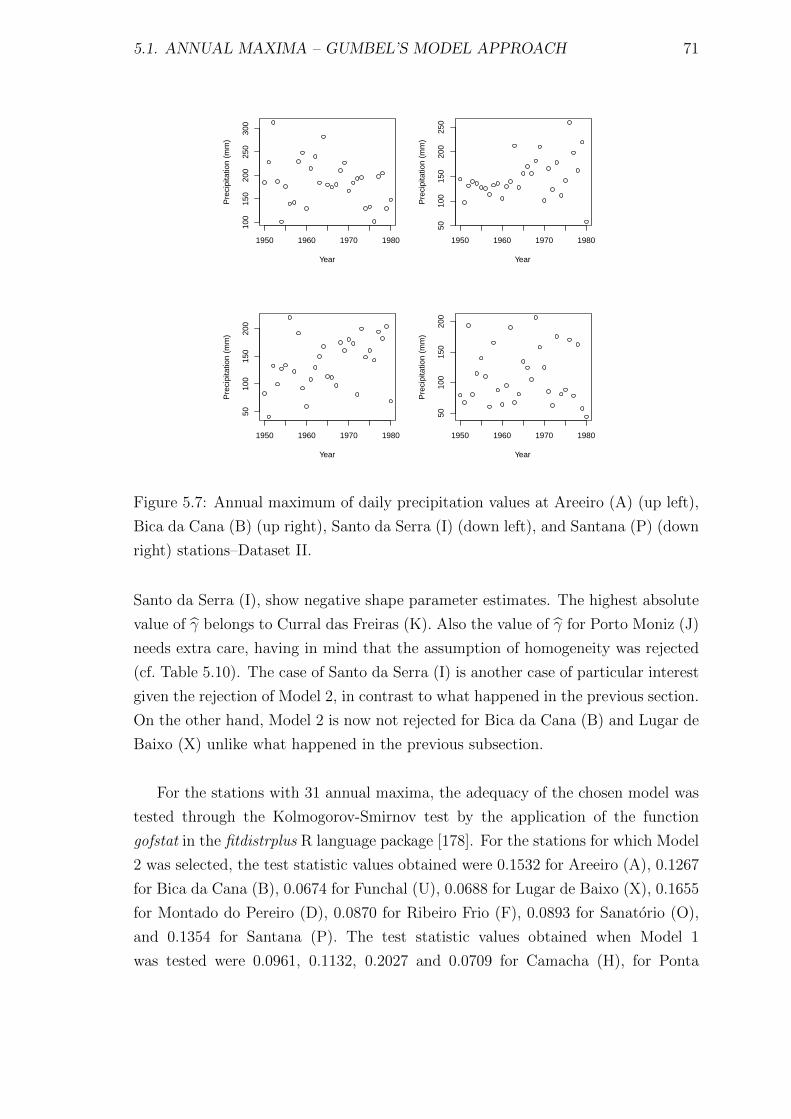
5.1. ANNUAL MAXIMA – GUMBEL’S MODEL APPROACH 71
1950 1960 1970 198010
015
020
025
030
0
Year
Pre
cipi
tatio
n (m
m)
1950 1960 1970 1980
5010
015
020
025
0
Year
Pre
cipi
tatio
n (m
m)
1950 1960 1970 1980
5010
015
020
0
Year
Pre
cipi
tatio
n (m
m)
1950 1960 1970 198050
100
150
200
Year
Pre
cipi
tatio
n (m
m)
Figure 5.7: Annual maximum of daily precipitation values at Areeiro (A) (up left),
Bica da Cana (B) (up right), Santo da Serra (I) (down left), and Santana (P) (down
right) stations–Dataset II.
Santo da Serra (I), show negative shape parameter estimates. The highest absolute
value of γ belongs to Curral das Freiras (K). Also the value of γ for Porto Moniz (J)
needs extra care, having in mind that the assumption of homogeneity was rejected
(cf. Table 5.10). The case of Santo da Serra (I) is another case of particular interest
given the rejection of Model 2, in contrast to what happened in the previous section.
On the other hand, Model 2 is now not rejected for Bica da Cana (B) and Lugar de
Baixo (X) unlike what happened in the previous subsection.
For the stations with 31 annual maxima, the adequacy of the chosen model was
tested through the Kolmogorov-Smirnov test by the application of the function
gofstat in the fitdistrplus R language package [178]. For the stations for which Model
2 was selected, the test statistic values obtained were 0.1532 for Areeiro (A), 0.1267
for Bica da Cana (B), 0.0674 for Funchal (U), 0.0688 for Lugar de Baixo (X), 0.1655
for Montado do Pereiro (D), 0.0870 for Ribeiro Frio (F), 0.0893 for Sanatorio (O),
and 0.1354 for Santana (P). The test statistic values obtained when Model 1
was tested were 0.0961, 0.1132, 0.2027 and 0.0709 for Camacha (H), for Ponta

72 CHAPTER 5. RESULTS AND DISCUSSION
1950 1960 1970 1980
2040
6080
100
Year
Pre
cipi
tatio
n (m
m)
1960 1965 1970 1975 1980
4060
8010
0
Year
Pre
cipi
tatio
n (m
m)
1950 1960 1970 1980
2040
6080
Year
Pre
cipi
tatio
n (m
m)
Figure 5.8: Annual maximum of daily precipitation values at Funchal (U) (up left),
Santa Catarina (V) (up right), and Lugar de Baixo (X) (down) stations–Dataset II.
Delgada (T), for Queimadas (G) and Santo da Serra (I), respectively. Therefore, for
each one rain gauge station, the data do not provide sufficient evidence to conclude
that the chosen model is not an appropriate model for modelling the respective
annual maxima, at a 0.05 significance level.
For the stations with shorter measurement periods, the adequacy of Model 2 was
tested by the application of the A2 modified statistic test discussed by Stephens [200]
and defined by expression (4.9), due to the sample sizes. The obtained values for
Poiso (C) and Encumeada (E), the remaining stations of Classes 1 and 2, were
0.267 and 0.351 respectively. The values of the A2 modified statistic test for the
remaining stations that belong to Class 3 is 0.246 for Ponta do Pargo (L), 0.246 for
Santo Antonio (M), 0.857 for Canhas (N) and 0.530 for Loural (Q). The values for
the stations with altitude below 300 meters are 0.332 for Bom Sucesso (R), 0.322
for Machico (S), 0.525 for Santa Catarina (V), 0.624 for Canical (W) and 0.211 for
Ribeira Brava (Y). At a 5% significance level, it appears that none of the observed
values of the test statistic, with the exception of Canhas (N) station, meets the
criteria for rejection, i.e., no value is greater than 0.757 ([200], Table 1). Thus, the
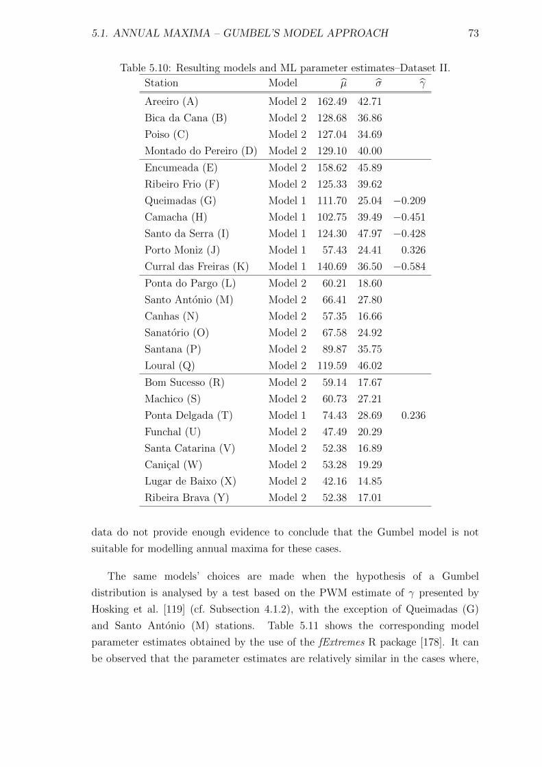
5.1. ANNUAL MAXIMA – GUMBEL’S MODEL APPROACH 73
Table 5.10: Resulting models and ML parameter estimates–Dataset II.
Station Model µ σ γ
Areeiro (A) Model 2 162.49 42.71
Bica da Cana (B) Model 2 128.68 36.86
Poiso (C) Model 2 127.04 34.69
Montado do Pereiro (D) Model 2 129.10 40.00
Encumeada (E) Model 2 158.62 45.89
Ribeiro Frio (F) Model 2 125.33 39.62
Queimadas (G) Model 1 111.70 25.04 −0.209
Camacha (H) Model 1 102.75 39.49 −0.451
Santo da Serra (I) Model 1 124.30 47.97 −0.428
Porto Moniz (J) Model 1 57.43 24.41 0.326
Curral das Freiras (K) Model 1 140.69 36.50 −0.584
Ponta do Pargo (L) Model 2 60.21 18.60
Santo Antonio (M) Model 2 66.41 27.80
Canhas (N) Model 2 57.35 16.66
Sanatorio (O) Model 2 67.58 24.92
Santana (P) Model 2 89.87 35.75
Loural (Q) Model 2 119.59 46.02
Bom Sucesso (R) Model 2 59.14 17.67
Machico (S) Model 2 60.73 27.21
Ponta Delgada (T) Model 1 74.43 28.69 0.236
Funchal (U) Model 2 47.49 20.29
Santa Catarina (V) Model 2 52.38 16.89
Canical (W) Model 2 53.28 19.29
Lugar de Baixo (X) Model 2 42.16 14.85
Ribeira Brava (Y) Model 2 52.38 17.01
data do not provide enough evidence to conclude that the Gumbel model is not
suitable for modelling annual maxima for these cases.
The same models’ choices are made when the hypothesis of a Gumbel
distribution is analysed by a test based on the PWM estimate of γ presented by
Hosking et al. [119] (cf. Subsection 4.1.2), with the exception of Queimadas (G)
and Santo Antonio (M) stations. Table 5.11 shows the corresponding model
parameter estimates obtained by the use of the fExtremes R package [178]. It can
be observed that the parameter estimates are relatively similar in the cases where,
74 CHAPTER 5. RESULTS AND DISCUSSION
independently of the method used, Model 2 is rejected. This is not the case
when Model 2 is chosen since the ML scale parameter estimates are much smaller
than the corresponding PWM estimates. The opposite happens with the location
parameter estimates, but in a less pronounced way. Although for the distributions
corresponding to these cases there is no significant evidence to choose Model 1
in opposition to Model 2, it is important to make the analysis of the situation
where only the GEV distribution is considered for the reasons already presented in
Subsection 5.1.1. The ML and PWM estimates for the location, scale and shape
parameters of the GEV distribution for each station in Classes 1 and 2 are displayed
in Table 5.12, while Table 5.13 shows the respective values for the ones that are in
Classes 3 and 4.
On the north side of the island, it can be observed that the estimated value of
the shape parameter for the GEV distribution is positive for the rain gauge stations
located nearest to the sea and it is negative for the three stations located in the
interior of the island, namely Bica da Cana (B), Encumeada (E) and Loural (Q).
For the rain gauge stations on the south side, there are cases of positive and negative
shape parameter estimates both in the interior and near the coast. The negative
shape parameter estimate enables the computation of an estimate of the upper end
point of the fitted distribution z0 through the expression z0 = µ − σ/γ. For the
stations that only appear in this subsection, z0 is equal to 333.71 mm for Montado
do Pereiro (D), 308.74 mm for Encumeada (E), 1421.46 mm for Ribeiro Frio (F),
231.51 mm for Queimadas (G), 190.31 mm for Camacha (H), 236.38 mm for Santo da
Serra (I), 203.19 mm for Curral das Freiras (K), 557.97 mm for Ponta do Pargo (L),
169.90 mm for Santo Antonio (M), 968.68 mm for Sanatorio (O), 510.69 mm for
Loural (Q), 123.80 mm for Bom Sucesso (R), and 96.64 mm for Canical (W).
If the PWM estimates are used, instead of the ML parameter ones, then the
value obtained for z0 is 336.45 mm for Montado do Pereiro (D), 327.85 mm for
Encumeada (E), 742.38 mm for Ribeiro Frio (F), 222.64 mm for Queimadas (G),
200.39 mm for Camacha (H), 259.49 mm for Santo da Serra (I), 205.95 mm for
Curral das Freiras (K), 397.23 mm for Ponta do Pargo (L), 166.08 mm for Santo
Antonio (M), 608.55 mm for Sanatorio (O), 419.31 mm for Loural (Q), 153.71 mm
for Bom Sucesso (R), and 142.34 mm for Canical (W).
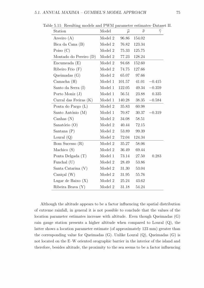
5.1. ANNUAL MAXIMA – GUMBEL’S MODEL APPROACH 75
Table 5.11: Resulting models and PWM parameter estimates–Dataset II.
Station Model µ σ γ
Areeiro (A) Model 2 96.86 154.02
Bica da Cana (B) Model 2 76.82 123.34
Poiso (C) Model 2 75.33 125.75
Montado do Pereiro (D) Model 2 77.23 128.24
Encumeada (E) Model 2 94.68 152.60
Ribeiro Frio (F) Model 2 74.75 127.66
Queimadas (G) Model 2 65.07 97.66
Camacha (H) Model 1 101.57 41.01 −0.415
Santo da Serra (I) Model 1 122.05 49.34 −0.359
Porto Moniz (J) Model 1 56.51 23.88 0.335
Curral das Freiras (K) Model 1 140.28 38.35 −0.584
Ponta do Pargo (L) Model 2 35.83 60.98
Santo Antonio (M) Model 1 70.87 30.37 −0.319
Canhas (N) Model 2 34.08 58.51
Sanatorio (O) Model 2 40.44 72.15
Santana (P) Model 2 53.89 99.39
Loural (Q) Model 2 72.04 124.34
Bom Sucesso (R) Model 2 35.27 58.06
Machico (S) Model 2 36.49 69.44
Ponta Delgada (T) Model 1 73.14 27.50 0.283
Funchal (U) Model 2 28.49 53.86
Santa Catarina (V) Model 2 31.30 53.04
Canical (W) Model 2 31.95 55.76
Lugar de Baixo (X) Model 2 25.24 43.62
Ribeira Brava (Y) Model 2 31.18 54.24
Although the altitude appears to be a factor influencing the spatial distribution
of extreme rainfall, in general it is not possible to conclude that the values of the
location parameter estimates increase with altitude. Even though Queimadas (G)
rain gauge station presents a higher altitude when compared to Loural (Q), the
latter shows a location parameter estimate (of approximately 123 mm) greater than
the corresponding value for Queimadas (G). Unlike Loural (Q), Queimadas (G) is
not located on the E–W oriented orographic barrier in the interior of the island and
therefore, besides altitude, the proximity to the sea seems to be a factor influencing

76 CHAPTER 5. RESULTS AND DISCUSSION
Table 5.12: GEV parameters estimates by ML and PWM (Classes 1 and 2)
Station Method µ σ γ
Areeiro (A) ML 166.07 44.22 −0.153
Areeiro (A) PWM 165.94 45.69 −0.167
Bica da Cana (B) ML 131.47 37.07 −0.143
Bica da Cana (B) PWM 129.40 34.15 −0.033
Poiso (C) ML 124.81 32.74 0.125
Poiso (C) PWM 125.15 36.50 0.045
Montado do Pereiro (D) ML 133.85 42.77 −0.214
Montado do Pereiro (D) PWM 133.45 45.27 −0.223
Encumeada (E) ML 167.24 49.10 −0.347
Encumeada (E) PWM 165.69 51.73 −0.319
Ribeiro Frio (F) ML 125.98 40.16 −0.031
Ribeiro Frio (F) PWM 126.04 43.76 −0.071
Queimadas (G) ML 111.70 25.04 −0.209
Queimadas (G) PWM 111.99 23.68 −0.214
Camacha (H) ML 102.75 39.49 −0.451
Camacha (H) PWM 101.57 41.01 −0.415
Santo da Serra (I) ML 124.30 47.97 −0.428
Santo da Serra (I) PWM 122.05 49.34 −0.359
Porto Moniz (J) ML 57.43 24.41 0.326
Porto Moniz (J) PWM 56.51 23.88 0.335
Curral das Freiras (K) ML 140.69 36.50 −0.584
Curral das Freiras (K) PWM 140.28 38.35 −0.584
the spatial distribution of extreme rainfall. Loural (Q) is also near the Encumeada
(E) rain gauge station, which presents the highest values for the location and scale
parameters estimates. Just below the values observed at Encumeada (E), are the
values corresponding to Areeiro (A), the rain gauge station located in the south
with the highest altitude in the island. Revealing the natural differences observed
on the windward and lee sides of any mountainous island, we have the rainfall data
from Sanatorio (O) and Santana (P) rain gauge stations. These stations have the
same altitude, but Sanatorio (O), which is located in the southern part of the island,
presents lower values for all the estimated values.

5.1. ANNUAL MAXIMA – GUMBEL’S MODEL APPROACH 77
Table 5.13: GEV parameters estimates by ML and PWM (Classes 3 and 4)
Station Method µ σ γ
Ponta do Pargo (L) ML 60.60 18.90 −0.038
Ponta do Pargo (L) PWM 60.34 20.55 −0.061
Santo Antonio (M) ML 70.86 29.02 −0.293
Santo Antonio (M) PWM 70.87 30.37 −0.319
Canhas (N) ML 52.64 11.52 0.637
Canhas (N) PWM 55.66 16.45 0.144
Sanatorio (O) ML 67.96 25.22 −0.028
Sanatorio (O) PWM 67.75 27.04 −0.050
Santana (P) ML 88.13 34.26 0.093
Santana (P) PWM 89.08 38.05 0.006
Loural (Q) ML 122.29 46.22 −0.119
Loural (Q) PWM 123.23 46.78 −0.158
Bom Sucesso (R) ML 62.18 19.41 −0.315
Bom Sucesso (R) PWM 60.86 19.87 −0.214
Machico (S) ML 60.49 27.06 0.016
Machico (S) PWM 59.80 27.62 0.030
Ponta Delgada (T) ML 74.43 28.69 0.236
Ponta Delgada (T) PWM 73.14 27.50 0.283
Funchal (U) ML 46.79 19.77 0.066
Funchal (U) PWM 46.35 20.32 0.070
Santa Catarina (V) ML 53.24 17.39 −0.094
Santa Catarina (V) PWM 52.80 17.81 −0.071
Canical (W) ML 62.35 28.32 −0.826
Canical (W) PWM 55.76 23.03 −0.266
Lugar de Baixo (X) ML 43.33 15.45 −0.145
Lugar de Baixo (X) PWM 42.68 15.66 −0.091
Ribeira Brava (Y) ML 51.74 16.55 0.070
Ribeira Brava (Y) PWM 51.43 17.28 0.060
The differences between the northern and the southern parts of Madeira Island
can also be found in terms of return levels. Illustrating these differences, Figures 5.9
and 5.10 present the diagnostic plots (cf. Subsection 4.1.3) for the GEV fit to Ribeira
Brava (Y) and Ponta Delgada (T) rain gauge data, respectively. The diagnostic
plots for Models 1 and 2 for the stations in Classes 1, 2, 3 and 4 are displayed in
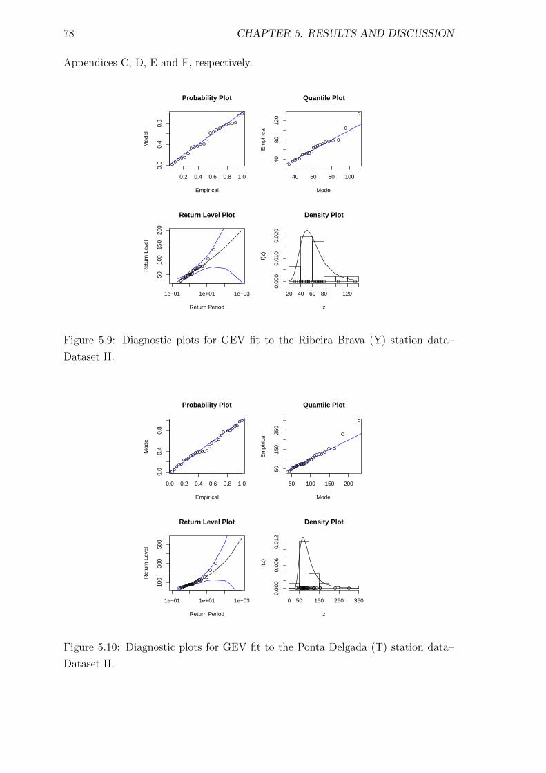
78 CHAPTER 5. RESULTS AND DISCUSSION
Appendices C, D, E and F, respectively.
0.2 0.4 0.6 0.8 1.0
0.0
0.4
0.8
Probability Plot
Empirical
Mod
el
40 60 80 100
4080
120
Quantile Plot
Model
Em
piric
al
1e−01 1e+01 1e+03
5010
015
020
0
Return Period
Ret
urn
Leve
l
Return Level Plot Density Plot
z
f(z)
20 40 60 80 120
0.00
00.
010
0.02
0
Figure 5.9: Diagnostic plots for GEV fit to the Ribeira Brava (Y) station data–
Dataset II.
0.0 0.2 0.4 0.6 0.8 1.0
0.0
0.4
0.8
Probability Plot
Empirical
Mod
el
50 100 150 200
5015
025
0
Quantile Plot
Model
Em
piric
al
1e−01 1e+01 1e+03
100
300
500
Return Period
Ret
urn
Leve
l
Return Level Plot Density Plot
z
f(z)
0 50 150 250 350
0.00
00.
006
0.01
2
Figure 5.10: Diagnostic plots for GEV fit to the Ponta Delgada (T) station data–
Dataset II.
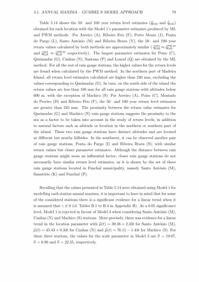
5.1. ANNUAL MAXIMA – GUMBEL’S MODEL APPROACH 79
Table 5.14 shows the 50– and 100–year return level estimates (q0.02 and q0.01)
obtained for each location with the Model 1’s parameter estimates produced by ML
and PWM methods. For Areeiro (A), Ribeiro Frio (F), Porto Moniz (J), Ponta
do Pargo (L), Santo Antonio (M) and Ribeira Brava (Y), the 50– and 100–year
return values calculated by both methods are approximately similar ( qML0.02 ≈ qPWM
0.02
and qML0.01 ≈ qPWM
0.01 respectively). The largest parameter estimates for Poiso (C),
Queimadas (G), Canhas (N), Santana (P) and Loural (Q) are obtained by the ML
method. For all the rest of rain gauge stations, the higher values for the return levels
are found when calculated by the PWM method. In the northern part of Madeira
Island, all return level estimates calculated are higher than 240 mm, excluding the
values corresponding to Queimadas (G). In turn, on the south side of the island the
return values are less than 180 mm for all rain gauge stations with altitudes below
600 m, with the exception of Machico (S). For Areeiro (A), Poiso (C), Montado
do Pereiro (D) and Ribeiro Frio (F), the 50– and 100–year return level estimates
are greater than 245 mm. The proximity between the return value estimates for
Queimadas (G) and Machico (N) rain gauge stations suggests the proximity to the
sea as a factor to be taken into account in the study of return levels, in addition
to natural factors such as altitude or location in the northern or southern part of
the island. These two rain gauge stations have distinct altitudes and are located
at different but nearby hillsides. In the southwest, it can be observed another pair
of rain gauge stations, Ponta do Pargo (I) and Ribeira Brava (S), with similar
return values but closer parameter estimates. Although the distance between rain
gauge stations might seem an influential factor, closer rain gauge stations do not
necessarily have similar return level estimates, as it is shown by the set of three
rain gauge stations located in Funchal municipality, namely Santo Antonio (M),
Sanatorio (K) and Funchal (P).
Recalling that the values presented in Table 5.14 were obtained using Model 1 for
modelling each station annual maxima, it is important to have in mind that for some
of the considered stations there is a significant evidence for a linear trend when it
is assumed that γ 6= 0 (cf. Tables B.1 to B.4 in Appendix B). At a 0.05 significance
level, Model 1 is rejected in favour of Model 3 when considering Santo Antonio (M),
Canhas (N) and Machico (S) stations. More precisely, there was evidence for a linear
trend in the location parameter with µ(t) = 39.38 + 2.33t for Santo Antonio (M),
µ(t) = 45.43 + 0.33t for Canhas (N) and µ(t) = 76.11 − 1.44t for Machico (S). For
these three stations, the values for the scale parameter in Model 3 are σ = 19.07,
σ = 6.90 and σ = 22.55, respectively.
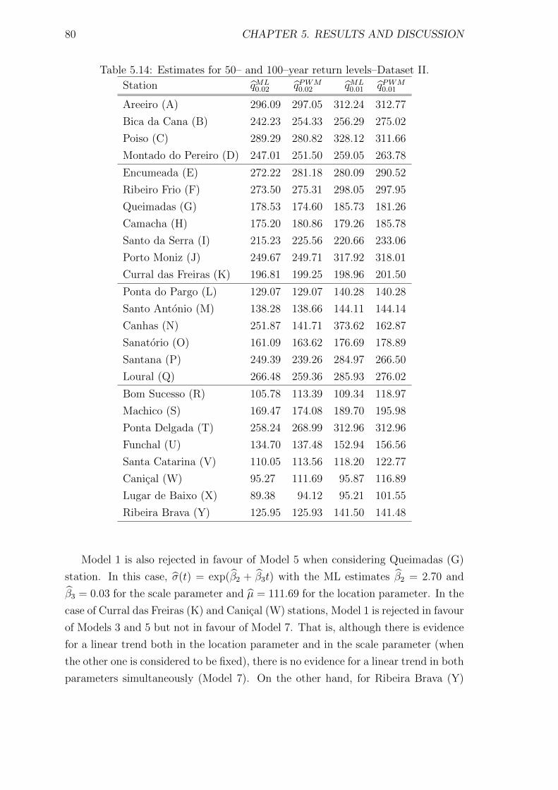
80 CHAPTER 5. RESULTS AND DISCUSSION
Table 5.14: Estimates for 50– and 100–year return levels–Dataset II.
Station qML0.02 qPWM
0.02 qML0.01 qPWM
0.01
Areeiro (A) 296.09 297.05 312.24 312.77
Bica da Cana (B) 242.23 254.33 256.29 275.02
Poiso (C) 289.29 280.82 328.12 311.66
Montado do Pereiro (D) 247.01 251.50 259.05 263.78
Encumeada (E) 272.22 281.18 280.09 290.52
Ribeiro Frio (F) 273.50 275.31 298.05 297.95
Queimadas (G) 178.53 174.60 185.73 181.26
Camacha (H) 175.20 180.86 179.26 185.78
Santo da Serra (I) 215.23 225.56 220.66 233.06
Porto Moniz (J) 249.67 249.71 317.92 318.01
Curral das Freiras (K) 196.81 199.25 198.96 201.50
Ponta do Pargo (L) 129.07 129.07 140.28 140.28
Santo Antonio (M) 138.28 138.66 144.11 144.14
Canhas (N) 251.87 141.71 373.62 162.87
Sanatorio (O) 161.09 163.62 176.69 178.89
Santana (P) 249.39 239.26 284.97 266.50
Loural (Q) 266.48 259.36 285.93 276.02
Bom Sucesso (R) 105.78 113.39 109.34 118.97
Machico (S) 169.47 174.08 189.70 195.98
Ponta Delgada (T) 258.24 268.99 312.96 312.96
Funchal (U) 134.70 137.48 152.94 156.56
Santa Catarina (V) 110.05 113.56 118.20 122.77
Canical (W) 95.27 111.69 95.87 116.89
Lugar de Baixo (X) 89.38 94.12 95.21 101.55
Ribeira Brava (Y) 125.95 125.93 141.50 141.48
Model 1 is also rejected in favour of Model 5 when considering Queimadas (G)
station. In this case, σ(t) = exp(β2 + β3t) with the ML estimates β2 = 2.70 and
β3 = 0.03 for the scale parameter and µ = 111.69 for the location parameter. In the
case of Curral das Freiras (K) and Canical (W) stations, Model 1 is rejected in favour
of Models 3 and 5 but not in favour of Model 7. That is, although there is evidence
for a linear trend both in the location parameter and in the scale parameter (when
the other one is considered to be fixed), there is no evidence for a linear trend in both
parameters simultaneously (Model 7). On the other hand, for Ribeira Brava (Y)
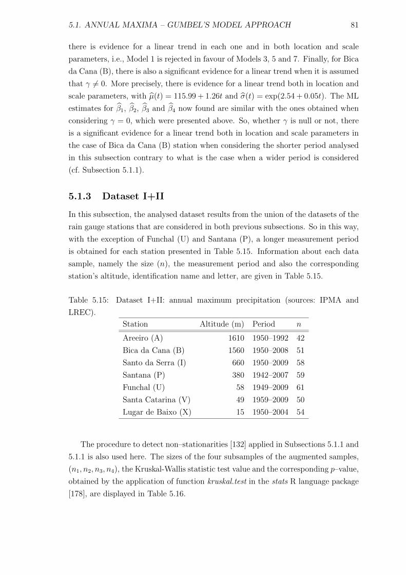
5.1. ANNUAL MAXIMA – GUMBEL’S MODEL APPROACH 81
there is evidence for a linear trend in each one and in both location and scale
parameters, i.e., Model 1 is rejected in favour of Models 3, 5 and 7. Finally, for Bica
da Cana (B), there is also a significant evidence for a linear trend when it is assumed
that γ 6= 0. More precisely, there is evidence for a linear trend both in location and
scale parameters, with µ(t) = 115.99 + 1.26t and σ(t) = exp(2.54 + 0.05t). The ML
estimates for β1, β2, β3 and β4 now found are similar with the ones obtained when
considering γ = 0, which were presented above. So, whether γ is null or not, there
is a significant evidence for a linear trend both in location and scale parameters in
the case of Bica da Cana (B) station when considering the shorter period analysed
in this subsection contrary to what is the case when a wider period is considered
(cf. Subsection 5.1.1).
5.1.3 Dataset I+II
In this subsection, the analysed dataset results from the union of the datasets of the
rain gauge stations that are considered in both previous subsections. So in this way,
with the exception of Funchal (U) and Santana (P), a longer measurement period
is obtained for each station presented in Table 5.15. Information about each data
sample, namely the size (n), the measurement period and also the corresponding
station’s altitude, identification name and letter, are given in Table 5.15.
Table 5.15: Dataset I+II: annual maximum precipitation (sources: IPMA and
LREC).
Station Altitude (m) Period n
Areeiro (A) 1610 1950–1992 42
Bica da Cana (B) 1560 1950–2008 51
Santo da Serra (I) 660 1950–2009 58
Santana (P) 380 1942–2007 59
Funchal (U) 58 1949–2009 61
Santa Catarina (V) 49 1959–2009 50
Lugar de Baixo (X) 15 1950–2004 54
The procedure to detect non–stationarities [132] applied in Subsections 5.1.1 and
5.1.1 is also used here. The sizes of the four subsamples of the augmented samples,
(n1, n2, n3, n4), the Kruskal-Wallis statistic test value and the corresponding p–value,
obtained by the application of function kruskal.test in the stats R language package
[178], are displayed in Table 5.16.
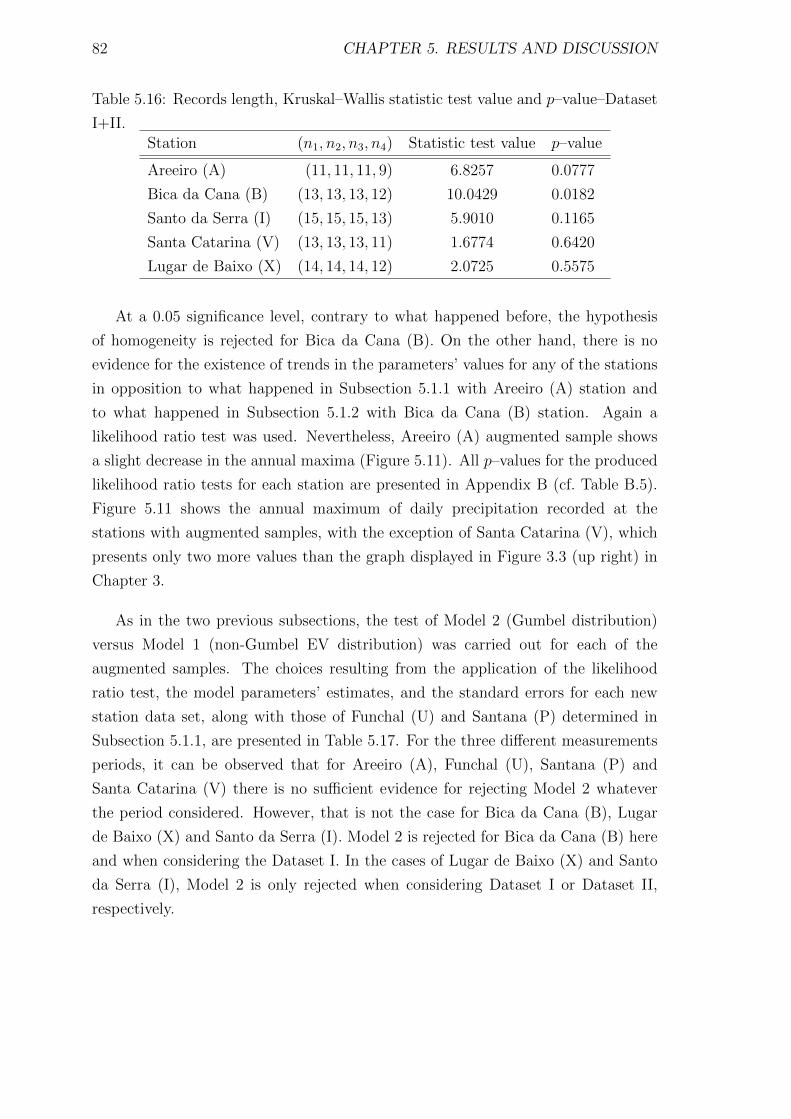
82 CHAPTER 5. RESULTS AND DISCUSSION
Table 5.16: Records length, Kruskal–Wallis statistic test value and p–value–Dataset
I+II.Station (n1, n2, n3, n4) Statistic test value p–value
Areeiro (A) (11, 11, 11, 9) 6.8257 0.0777
Bica da Cana (B) (13, 13, 13, 12) 10.0429 0.0182
Santo da Serra (I) (15, 15, 15, 13) 5.9010 0.1165
Santa Catarina (V) (13, 13, 13, 11) 1.6774 0.6420
Lugar de Baixo (X) (14, 14, 14, 12) 2.0725 0.5575
At a 0.05 significance level, contrary to what happened before, the hypothesis
of homogeneity is rejected for Bica da Cana (B). On the other hand, there is no
evidence for the existence of trends in the parameters’ values for any of the stations
in opposition to what happened in Subsection 5.1.1 with Areeiro (A) station and
to what happened in Subsection 5.1.2 with Bica da Cana (B) station. Again a
likelihood ratio test was used. Nevertheless, Areeiro (A) augmented sample shows
a slight decrease in the annual maxima (Figure 5.11). All p–values for the produced
likelihood ratio tests for each station are presented in Appendix B (cf. Table B.5).
Figure 5.11 shows the annual maximum of daily precipitation recorded at the
stations with augmented samples, with the exception of Santa Catarina (V), which
presents only two more values than the graph displayed in Figure 3.3 (up right) in
Chapter 3.
As in the two previous subsections, the test of Model 2 (Gumbel distribution)
versus Model 1 (non-Gumbel EV distribution) was carried out for each of the
augmented samples. The choices resulting from the application of the likelihood
ratio test, the model parameters’ estimates, and the standard errors for each new
station data set, along with those of Funchal (U) and Santana (P) determined in
Subsection 5.1.1, are presented in Table 5.17. For the three different measurements
periods, it can be observed that for Areeiro (A), Funchal (U), Santana (P) and
Santa Catarina (V) there is no sufficient evidence for rejecting Model 2 whatever
the period considered. However, that is not the case for Bica da Cana (B), Lugar
de Baixo (X) and Santo da Serra (I). Model 2 is rejected for Bica da Cana (B) here
and when considering the Dataset I. In the cases of Lugar de Baixo (X) and Santo
da Serra (I), Model 2 is only rejected when considering Dataset I or Dataset II,
respectively.
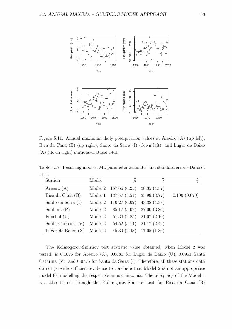
5.1. ANNUAL MAXIMA – GUMBEL’S MODEL APPROACH 83
1950 1970 1990
100
200
300
YearP
reci
pita
tion
(mm
)
1950 1970 1990 2010
5010
020
0
Year
Pre
cipi
tatio
n (m
m)
1950 1970 1990 2010
5015
025
0
Year
Pre
cipi
tatio
n (m
m)
1950 1970 1990
2060
100
140
YearP
reci
pita
tion
(mm
)
Figure 5.11: Annual maximum daily precipitation values at Areeiro (A) (up left),
Bica da Cana (B) (up right), Santo da Serra (I) (down left), and Lugar de Baixo
(X) (down right) stations–Dataset I+II.
Table 5.17: Resulting models, ML parameter estimates and standard errors–Dataset
I+II.Station Model µ σ γ
Areeiro (A) Model 2 157.66 (6.25) 38.35 (4.57)
Bica da Cana (B) Model 1 137.57 (5.51) 35.99 (3.77) −0.190 (0.079)
Santo da Serra (I) Model 2 110.27 (6.02) 43.38 (4.38)
Santana (P) Model 2 85.17 (5.07) 37.00 (3.86)
Funchal (U) Model 2 51.34 (2.85) 21.07 (2.10)
Santa Catarina (V) Model 2 54.52 (3.14) 21.17 (2.42)
Lugar de Baixo (X) Model 2 45.39 (2.43) 17.05 (1.86)
The Kolmogorov-Smirnov test statistic value obtained, when Model 2 was
tested, is 0.1025 for Areeiro (A), 0.0681 for Lugar de Baixo (U), 0.0951 Santa
Catarina (V), and 0.0725 for Santo da Serra (I). Therefore, all these stations data
do not provide sufficient evidence to conclude that Model 2 is not an appropriate
model for modelling the respective annual maxima. The adequacy of the Model 1
was also tested through the Kolmogorov-Smirnov test for Bica da Cana (B)
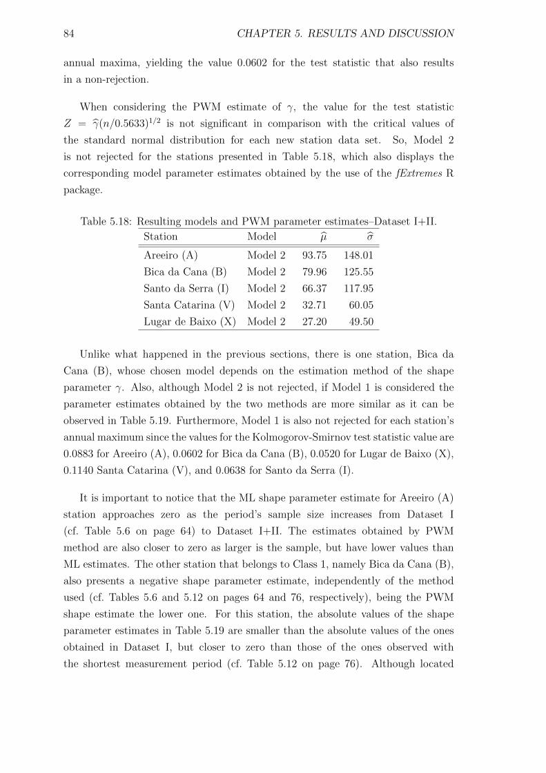
84 CHAPTER 5. RESULTS AND DISCUSSION
annual maxima, yielding the value 0.0602 for the test statistic that also results
in a non-rejection.
When considering the PWM estimate of γ, the value for the test statistic
Z = γ(n/0.5633)1/2 is not significant in comparison with the critical values of
the standard normal distribution for each new station data set. So, Model 2
is not rejected for the stations presented in Table 5.18, which also displays the
corresponding model parameter estimates obtained by the use of the fExtremes R
package.
Table 5.18: Resulting models and PWM parameter estimates–Dataset I+II.
Station Model µ σ
Areeiro (A) Model 2 93.75 148.01
Bica da Cana (B) Model 2 79.96 125.55
Santo da Serra (I) Model 2 66.37 117.95
Santa Catarina (V) Model 2 32.71 60.05
Lugar de Baixo (X) Model 2 27.20 49.50
Unlike what happened in the previous sections, there is one station, Bica da
Cana (B), whose chosen model depends on the estimation method of the shape
parameter γ. Also, although Model 2 is not rejected, if Model 1 is considered the
parameter estimates obtained by the two methods are more similar as it can be
observed in Table 5.19. Furthermore, Model 1 is also not rejected for each station’s
annual maximum since the values for the Kolmogorov-Smirnov test statistic value are
0.0883 for Areeiro (A), 0.0602 for Bica da Cana (B), 0.0520 for Lugar de Baixo (X),
0.1140 Santa Catarina (V), and 0.0638 for Santo da Serra (I).
It is important to notice that the ML shape parameter estimate for Areeiro (A)
station approaches zero as the period’s sample size increases from Dataset I
(cf. Table 5.6 on page 64) to Dataset I+II. The estimates obtained by PWM
method are also closer to zero as larger is the sample, but have lower values than
ML estimates. The other station that belongs to Class 1, namely Bica da Cana (B),
also presents a negative shape parameter estimate, independently of the method
used (cf. Tables 5.6 and 5.12 on pages 64 and 76, respectively), being the PWM
shape estimate the lower one. For this station, the absolute values of the shape
parameter estimates in Table 5.19 are smaller than the absolute values of the ones
obtained in Dataset I, but closer to zero than those of the ones observed with
the shortest measurement period (cf. Table 5.12 on page 76). Although located
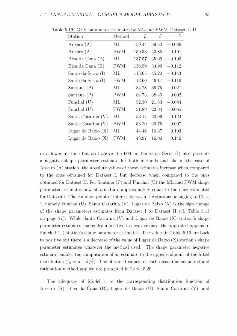
5.1. ANNUAL MAXIMA – GUMBEL’S MODEL APPROACH 85
Table 5.19: GEV parameter estimates by ML and PWM–Dataset I+II.
Station Method µ σ γ
Areeiro (A) ML 159.44 39.32 −0.086
Areeiro (A) PWM 159.33 40.85 −0.101
Bica da Cana (B) ML 137.57 35.99 −0.190
Bica da Cana (B) PWM 136.59 34.99 −0.142
Santo da Serra (I) ML 113.65 45.20 −0.143
Santo da Serra (I) PWM 112.60 46.17 −0.116
Santana (P) ML 84.78 36.75 0.021
Santana (P) PWM 84.73 38.40 0.002
Funchal (U) ML 52.30 21.63 −0.084
Funchal (U) PWM 51.89 22.04 −0.065
Santa Catarina (V) ML 53.14 20.06 0.124
Santa Catarina (V) PWM 53.20 20.75 0.097
Lugar de Baixo (X) ML 44.46 16.37 0.103
Lugar de Baixo (X) PWM 43.97 16.00 0.140
in a lower altitude but still above the 600 m, Santo da Serra (I) also presents
a negative shape parameter estimate for both methods and like in the case of
Areeiro (A) station, the absolute values of these estimates increase when compared
to the ones obtained for Dataset I, but decrease when compared to the ones
obtained for Dataset II. For Santana (P) and Funchal (U) the ML and PWM shape
parameter estimates now obtained are approximately equal to the ones estimated
for Dataset I. The common point of interest between the stations belonging to Class
1, namely Funchal (U), Santa Catarina (V), Lugar de Baixo (X) is the sign change
of the shape parameters estimates from Dataset I to Dataset II (cf. Table 5.13
on page 77). While Santa Catarina (V) and Lugar de Baixo (X) station’s shape
parameter estimates change from positive to negative ones, the opposite happens to
Funchal (U) station’s shape parameter estimates. The values in Table 5.19 are back
to positive but there is a decrease of the value of Lugar de Baixo (X) station’s shape
parameter estimates whatever the method used. The shape parameter negative
estimate enables the computation of an estimate to the upper endpoint of the fitted
distribution (z0 = µ− σ/γ). The obtained values for each measurement period and
estimation method applied are presented in Table 5.20.
The adequacy of Model 1 to the corresponding distribution function of
Areeiro (A), Bica da Cana (B), Lugar de Baixo (U), Santa Catarina (V), and
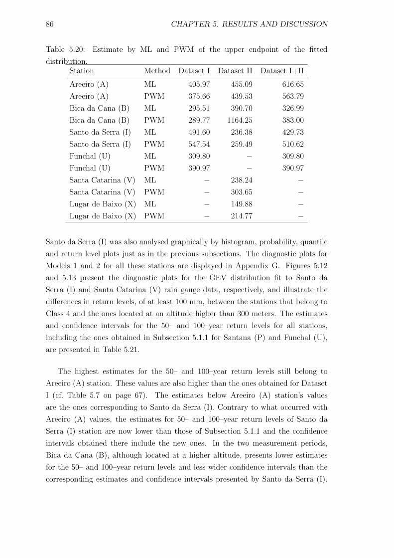
86 CHAPTER 5. RESULTS AND DISCUSSION
Table 5.20: Estimate by ML and PWM of the upper endpoint of the fitted
distribution.Station Method Dataset I Dataset II Dataset I+II
Areeiro (A) ML 405.97 455.09 616.65
Areeiro (A) PWM 375.66 439.53 563.79
Bica da Cana (B) ML 295.51 390.70 326.99
Bica da Cana (B) PWM 289.77 1164.25 383.00
Santo da Serra (I) ML 491.60 236.38 429.73
Santo da Serra (I) PWM 547.54 259.49 510.62
Funchal (U) ML 309.80 − 309.80
Funchal (U) PWM 390.97 − 390.97
Santa Catarina (V) ML − 238.24 −Santa Catarina (V) PWM − 303.65 −Lugar de Baixo (X) ML − 149.88 −Lugar de Baixo (X) PWM − 214.77 −
Santo da Serra (I) was also analysed graphically by histogram, probability, quantile
and return level plots just as in the previous subsections. The diagnostic plots for
Models 1 and 2 for all these stations are displayed in Appendix G. Figures 5.12
and 5.13 present the diagnostic plots for the GEV distribution fit to Santo da
Serra (I) and Santa Catarina (V) rain gauge data, respectively, and illustrate the
differences in return levels, of at least 100 mm, between the stations that belong to
Class 4 and the ones located at an altitude higher than 300 meters. The estimates
and confidence intervals for the 50– and 100–year return levels for all stations,
including the ones obtained in Subsection 5.1.1 for Santana (P) and Funchal (U),
are presented in Table 5.21.
The highest estimates for the 50– and 100–year return levels still belong to
Areeiro (A) station. These values are also higher than the ones obtained for Dataset
I (cf. Table 5.7 on page 67). The estimates below Areeiro (A) station’s values
are the ones corresponding to Santo da Serra (I). Contrary to what occurred with
Areeiro (A) values, the estimates for 50– and 100–year return levels of Santo da
Serra (I) station are now lower than those of Subsection 5.1.1 and the confidence
intervals obtained there include the new ones. In the two measurement periods,
Bica da Cana (B), although located at a higher altitude, presents lower estimates
for the 50– and 100–year return levels and less wider confidence intervals than the
corresponding estimates and confidence intervals presented by Santo da Serra (I).
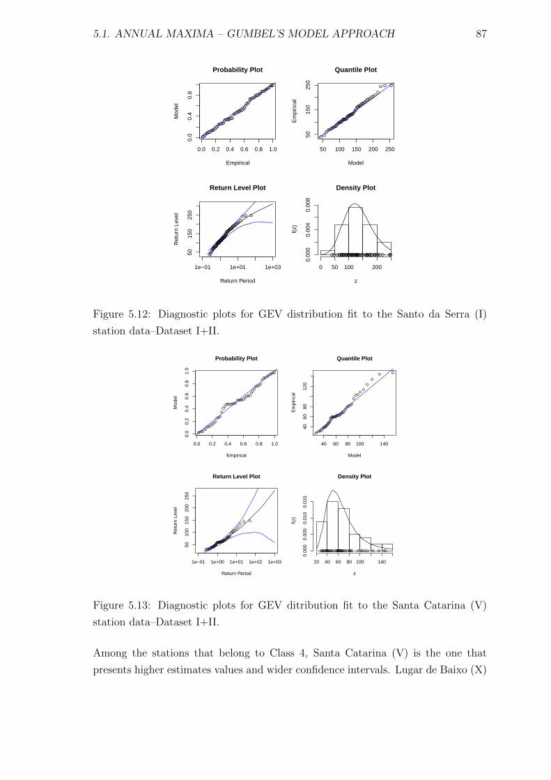
5.1. ANNUAL MAXIMA – GUMBEL’S MODEL APPROACH 87
0.0 0.2 0.4 0.6 0.8 1.0
0.0
0.4
0.8
Probability Plot
Empirical
Mod
el
50 100 150 200 250
5015
025
0
Quantile Plot
Model
Em
piric
al
1e−01 1e+01 1e+03
5015
025
0
Return Period
Ret
urn
Leve
l
Return Level Plot Density Plot
z
f(z)
0 50 100 200
0.00
00.
004
0.00
8
Figure 5.12: Diagnostic plots for GEV distribution fit to the Santo da Serra (I)
station data–Dataset I+II.
0.0 0.2 0.4 0.6 0.8 1.0
0.0
0.2
0.4
0.6
0.8
1.0
Probability Plot
Empirical
Mod
el
40 60 80 100 140
4060
8012
0
Quantile Plot
Model
Em
piric
al
1e−01 1e+00 1e+01 1e+02 1e+03
5010
015
020
025
0
Return Period
Ret
urn
Leve
l
Return Level Plot Density Plot
z
f(z)
20 40 60 80 100 140
0.00
00.
005
0.01
00.
015
Figure 5.13: Diagnostic plots for GEV ditribution fit to the Santa Catarina (V)
station data–Dataset I+II.
Among the stations that belong to Class 4, Santa Catarina (V) is the one that
presents higher estimates values and wider confidence intervals. Lugar de Baixo (X)
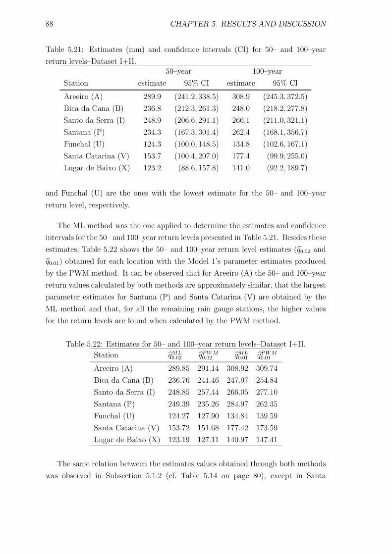
88 CHAPTER 5. RESULTS AND DISCUSSION
Table 5.21: Estimates (mm) and confidence intervals (CI) for 50– and 100–year
return levels–Dataset I+II.50–year 100–year
Station estimate 95% CI estimate 95% CI
Areeiro (A) 289.9 (241.2, 338.5) 308.9 (245.3, 372.5)
Bica da Cana (B) 236.8 (212.3, 261.3) 248.0 (218.2, 277.8)
Santo da Serra (I) 248.9 (206.6, 291.1) 266.1 (211.0, 321.1)
Santana (P) 234.3 (167.3, 301.4) 262.4 (168.1, 356.7)
Funchal (U) 124.3 (100.0, 148.5) 134.8 (102.6, 167.1)
Santa Catarina (V) 153.7 (100.4, 207.0) 177.4 (99.9, 255.0)
Lugar de Baixo (X) 123.2 (88.6, 157.8) 141.0 (92.2, 189.7)
and Funchal (U) are the ones with the lowest estimate for the 50– and 100–year
return level, respectively.
The ML method was the one applied to determine the estimates and confidence
intervals for the 50– and 100–year return levels presented in Table 5.21. Besides these
estimates, Table 5.22 shows the 50– and 100–year return level estimates (q0.02 and
q0.01) obtained for each location with the Model 1’s parameter estimates produced
by the PWM method. It can be observed that for Areeiro (A) the 50– and 100–year
return values calculated by both methods are approximately similar, that the largest
parameter estimates for Santana (P) and Santa Catarina (V) are obtained by the
ML method and that, for all the remaining rain gauge stations, the higher values
for the return levels are found when calculated by the PWM method.
Table 5.22: Estimates for 50– and 100–year return levels–Dataset I+II.
Station qML0.02 qPWM
0.02 qML0.01 qPWM
0.01
Areeiro (A) 289.85 291.14 308.92 309.74
Bica da Cana (B) 236.76 241.46 247.97 254.84
Santo da Serra (I) 248.85 257.44 266.05 277.10
Santana (P) 249.39 235.26 284.97 262.35
Funchal (U) 124.27 127.90 134.84 139.59
Santa Catarina (V) 153.72 151.68 177.42 173.59
Lugar de Baixo (X) 123.19 127.11 140.97 147.41
The same relation between the estimates values obtained through both methods
was observed in Subsection 5.1.2 (cf. Table 5.14 on page 80), except in Santa
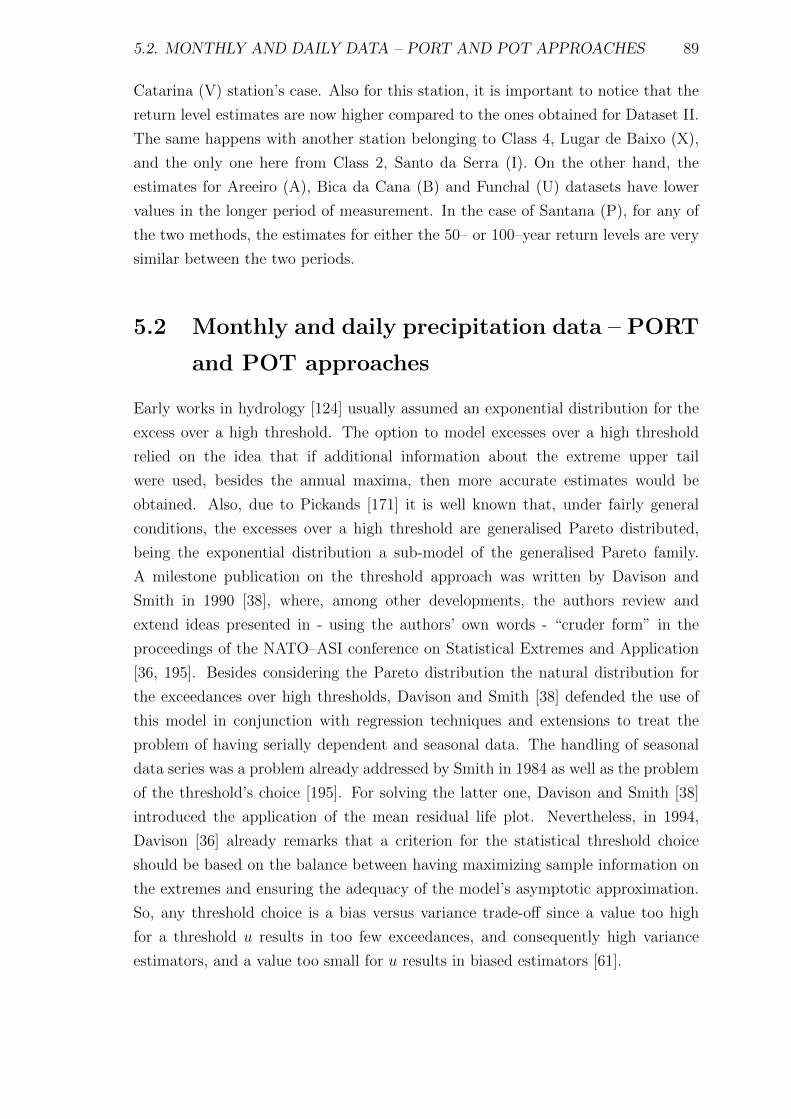
5.2. MONTHLY AND DAILY DATA – PORT AND POT APPROACHES 89
Catarina (V) station’s case. Also for this station, it is important to notice that the
return level estimates are now higher compared to the ones obtained for Dataset II.
The same happens with another station belonging to Class 4, Lugar de Baixo (X),
and the only one here from Class 2, Santo da Serra (I). On the other hand, the
estimates for Areeiro (A), Bica da Cana (B) and Funchal (U) datasets have lower
values in the longer period of measurement. In the case of Santana (P), for any of
the two methods, the estimates for either the 50– or 100–year return levels are very
similar between the two periods.
5.2 Monthly and daily precipitation data – PORT
and POT approaches
Early works in hydrology [124] usually assumed an exponential distribution for the
excess over a high threshold. The option to model excesses over a high threshold
relied on the idea that if additional information about the extreme upper tail
were used, besides the annual maxima, then more accurate estimates would be
obtained. Also, due to Pickands [171] it is well known that, under fairly general
conditions, the excesses over a high threshold are generalised Pareto distributed,
being the exponential distribution a sub-model of the generalised Pareto family.
A milestone publication on the threshold approach was written by Davison and
Smith in 1990 [38], where, among other developments, the authors review and
extend ideas presented in - using the authors’ own words - “cruder form” in the
proceedings of the NATO–ASI conference on Statistical Extremes and Application
[36, 195]. Besides considering the Pareto distribution the natural distribution for
the exceedances over high thresholds, Davison and Smith [38] defended the use of
this model in conjunction with regression techniques and extensions to treat the
problem of having serially dependent and seasonal data. The handling of seasonal
data series was a problem already addressed by Smith in 1984 as well as the problem
of the threshold’s choice [195]. For solving the latter one, Davison and Smith [38]
introduced the application of the mean residual life plot. Nevertheless, in 1994,
Davison [36] already remarks that a criterion for the statistical threshold choice
should be based on the balance between having maximizing sample information on
the extremes and ensuring the adequacy of the model’s asymptotic approximation.
So, any threshold choice is a bias versus variance trade-off since a value too high
for a threshold u results in too few exceedances, and consequently high variance
estimators, and a value too small for u results in biased estimators [61].
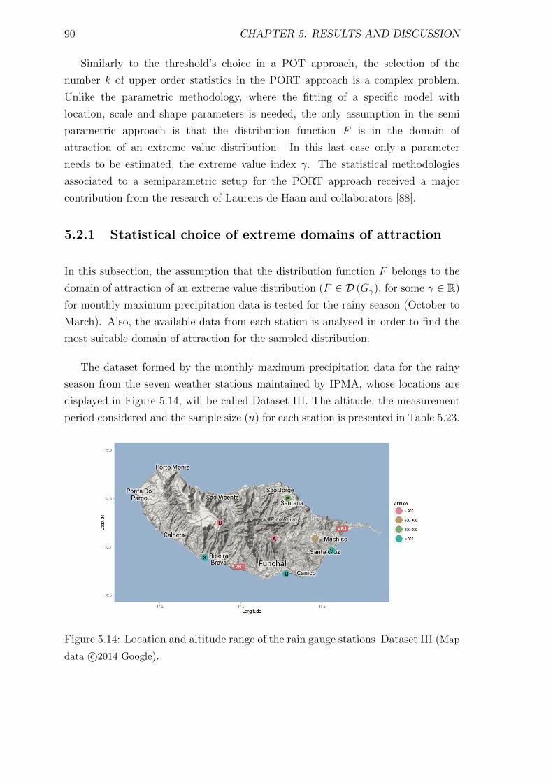
90 CHAPTER 5. RESULTS AND DISCUSSION
Similarly to the threshold’s choice in a POT approach, the selection of the
number k of upper order statistics in the PORT approach is a complex problem.
Unlike the parametric methodology, where the fitting of a specific model with
location, scale and shape parameters is needed, the only assumption in the semi
parametric approach is that the distribution function F is in the domain of
attraction of an extreme value distribution. In this last case only a parameter
needs to be estimated, the extreme value index γ. The statistical methodologies
associated to a semiparametric setup for the PORT approach received a major
contribution from the research of Laurens de Haan and collaborators [88].
5.2.1 Statistical choice of extreme domains of attraction
In this subsection, the assumption that the distribution function F belongs to the
domain of attraction of an extreme value distribution (F ∈ D (Gγ), for some γ ∈ R)
for monthly maximum precipitation data is tested for the rainy season (October to
March). Also, the available data from each station is analysed in order to find the
most suitable domain of attraction for the sampled distribution.
The dataset formed by the monthly maximum precipitation data for the rainy
season from the seven weather stations maintained by IPMA, whose locations are
displayed in Figure 5.14, will be called Dataset III. The altitude, the measurement
period considered and the sample size (n) for each station is presented in Table 5.23.
Figure 5.14: Location and altitude range of the rain gauge stations–Dataset III (Map
data c©2014 Google).
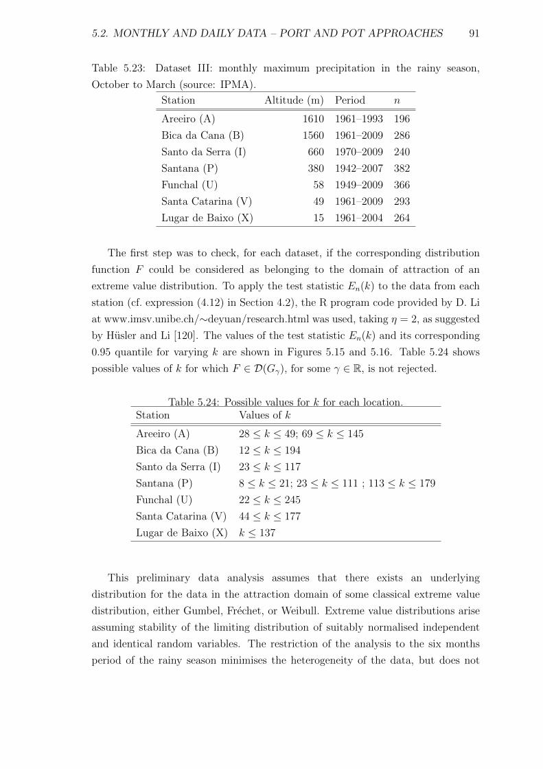
5.2. MONTHLY AND DAILY DATA – PORT AND POT APPROACHES 91
Table 5.23: Dataset III: monthly maximum precipitation in the rainy season,
October to March (source: IPMA).
Station Altitude (m) Period n
Areeiro (A) 1610 1961–1993 196
Bica da Cana (B) 1560 1961–2009 286
Santo da Serra (I) 660 1970–2009 240
Santana (P) 380 1942–2007 382
Funchal (U) 58 1949–2009 366
Santa Catarina (V) 49 1961–2009 293
Lugar de Baixo (X) 15 1961–2004 264
The first step was to check, for each dataset, if the corresponding distribution
function F could be considered as belonging to the domain of attraction of an
extreme value distribution. To apply the test statistic En(k) to the data from each
station (cf. expression (4.12) in Section 4.2), the R program code provided by D. Li
at www.imsv.unibe.ch/∼deyuan/research.html was used, taking η = 2, as suggested
by Husler and Li [120]. The values of the test statistic En(k) and its corresponding
0.95 quantile for varying k are shown in Figures 5.15 and 5.16. Table 5.24 shows
possible values of k for which F ∈ D(Gγ), for some γ ∈ R, is not rejected.
Table 5.24: Possible values for k for each location.Station Values of k
Areeiro (A) 28 ≤ k ≤ 49; 69 ≤ k ≤ 145
Bica da Cana (B) 12 ≤ k ≤ 194
Santo da Serra (I) 23 ≤ k ≤ 117
Santana (P) 8 ≤ k ≤ 21; 23 ≤ k ≤ 111 ; 113 ≤ k ≤ 179
Funchal (U) 22 ≤ k ≤ 245
Santa Catarina (V) 44 ≤ k ≤ 177
Lugar de Baixo (X) k ≤ 137
This preliminary data analysis assumes that there exists an underlying
distribution for the data in the attraction domain of some classical extreme value
distribution, either Gumbel, Frechet, or Weibull. Extreme value distributions arise
assuming stability of the limiting distribution of suitably normalised independent
and identical random variables. The restriction of the analysis to the six months
period of the rainy season minimises the heterogeneity of the data, but does not
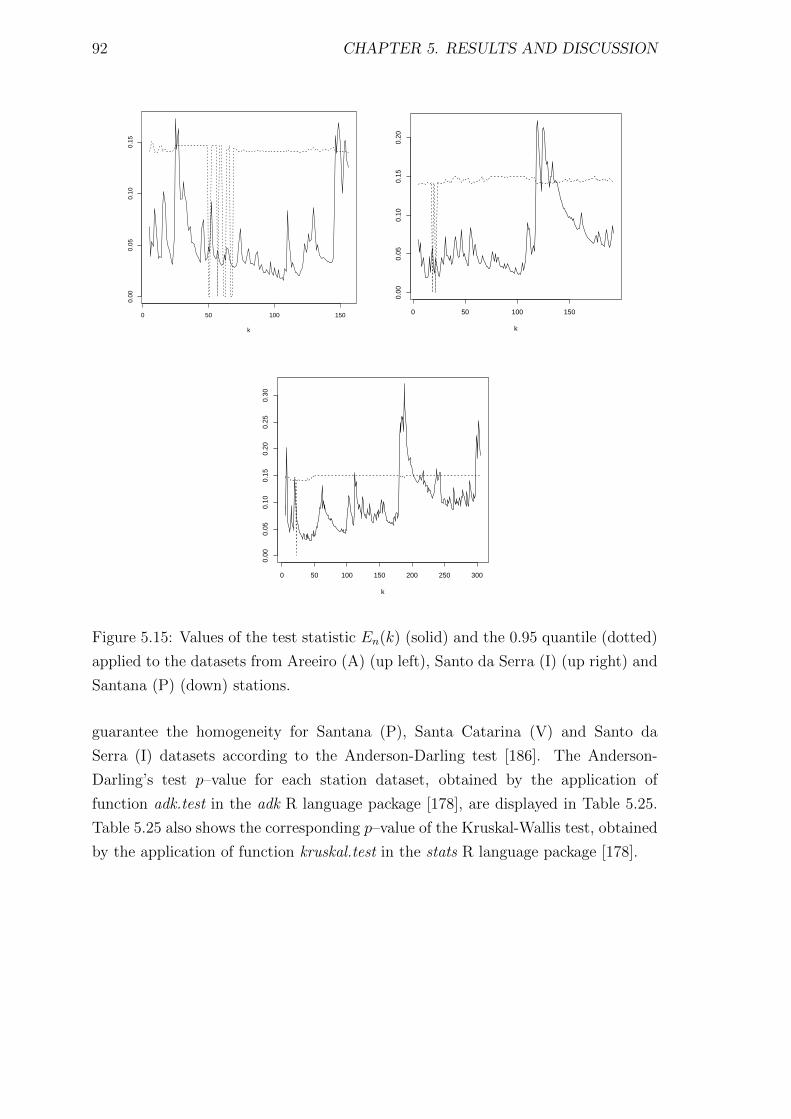
92 CHAPTER 5. RESULTS AND DISCUSSION
0 50 100 150
0.00
0.05
0.10
0.15
k
0 50 100 150
0.00
0.05
0.10
0.15
0.20
k
0 50 100 150 200 250 300
0.00
0.05
0.10
0.15
0.20
0.25
0.30
k
Figure 5.15: Values of the test statistic En(k) (solid) and the 0.95 quantile (dotted)
applied to the datasets from Areeiro (A) (up left), Santo da Serra (I) (up right) and
Santana (P) (down) stations.
guarantee the homogeneity for Santana (P), Santa Catarina (V) and Santo da
Serra (I) datasets according to the Anderson-Darling test [186]. The Anderson-
Darling’s test p–value for each station dataset, obtained by the application of
function adk.test in the adk R language package [178], are displayed in Table 5.25.
Table 5.25 also shows the corresponding p–value of the Kruskal-Wallis test, obtained
by the application of function kruskal.test in the stats R language package [178].
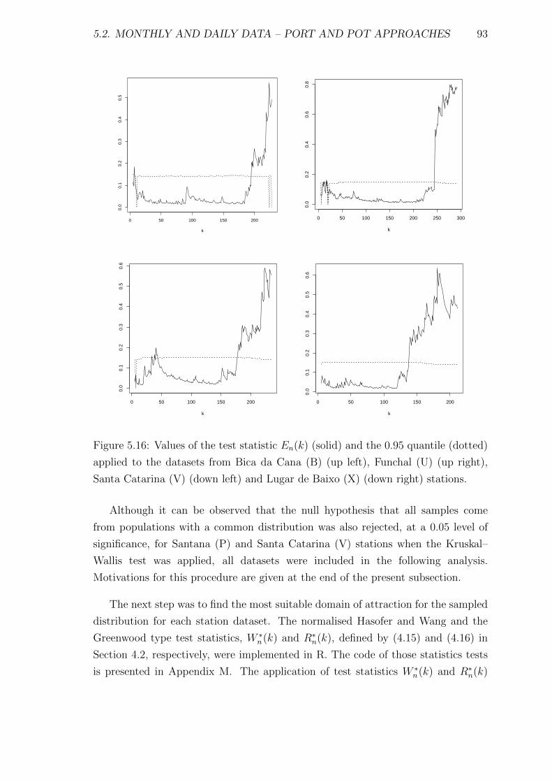
5.2. MONTHLY AND DAILY DATA – PORT AND POT APPROACHES 93
0 50 100 150 200
0.0
0.1
0.2
0.3
0.4
0.5
k
0 50 100 150 200 250 300
0.0
0.2
0.4
0.6
0.8
k
0 50 100 150 200
0.0
0.1
0.2
0.3
0.4
0.5
0.6
k
0 50 100 150 200
0.0
0.1
0.2
0.3
0.4
0.5
0.6
k
Figure 5.16: Values of the test statistic En(k) (solid) and the 0.95 quantile (dotted)
applied to the datasets from Bica da Cana (B) (up left), Funchal (U) (up right),
Santa Catarina (V) (down left) and Lugar de Baixo (X) (down right) stations.
Although it can be observed that the null hypothesis that all samples come
from populations with a common distribution was also rejected, at a 0.05 level of
significance, for Santana (P) and Santa Catarina (V) stations when the Kruskal–
Wallis test was applied, all datasets were included in the following analysis.
Motivations for this procedure are given at the end of the present subsection.
The next step was to find the most suitable domain of attraction for the sampled
distribution for each station dataset. The normalised Hasofer and Wang and the
Greenwood type test statistics, W ∗n(k) and R∗n(k), defined by (4.15) and (4.16) in
Section 4.2, respectively, were implemented in R. The code of those statistics tests
is presented in Appendix M. The application of test statistics W ∗n(k) and R∗n(k)
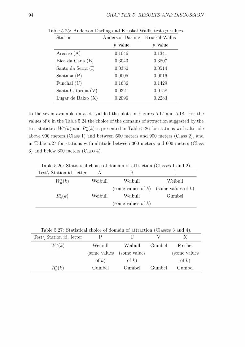
94 CHAPTER 5. RESULTS AND DISCUSSION
Table 5.25: Anderson-Darling and Kruskal-Wallis tests p–values.
Station Anderson-Darling Kruskal-Wallis
p–value p–value
Areeiro (A) 0.1046 0.1341
Bica da Cana (B) 0.3043 0.3807
Santo da Serra (I) 0.0350 0.0514
Santana (P) 0.0005 0.0016
Funchal (U) 0.1636 0.1429
Santa Catarina (V) 0.0327 0.0158
Lugar de Baixo (X) 0.2096 0.2283
to the seven available datasets yielded the plots in Figures 5.17 and 5.18. For the
values of k in the Table 5.24 the choice of the domains of attraction suggested by the
test statistics W ∗n(k) and R∗n(k) is presented in Table 5.26 for stations with altitude
above 900 meters (Class 1) and between 600 meters and 900 meters (Class 2), and
in Table 5.27 for stations with altitude between 300 meters and 600 meters (Class
3) and below 300 meters (Class 4).
Table 5.26: Statistical choice of domain of attraction (Classes 1 and 2).
Test\ Station id. letter A B I
W ∗n(k) Weibull Weibull Weibull
(some values of k) (some values of k)
R∗n(k) Weibull Weibull Gumbel
(some values of k)
Table 5.27: Statistical choice of domain of attraction (Classes 3 and 4).
Test\ Station id. letter P U V X
W ∗n(k) Weibull Weibull Gumbel Frechet
(some values (some values (some values
of k) of k) of k)
R∗n(k) Gumbel Gumbel Gumbel Gumbel
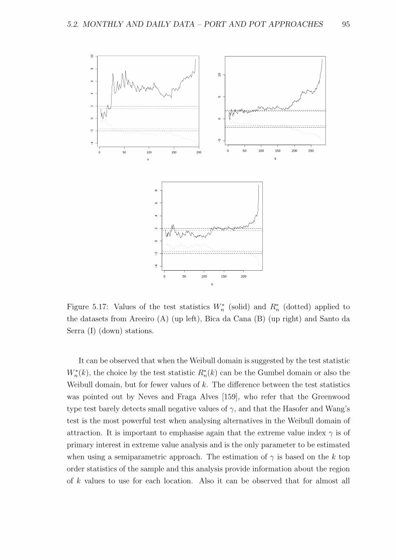
5.2. MONTHLY AND DAILY DATA – PORT AND POT APPROACHES 95
0 50 100 150 200
−4
−2
02
46
810
k
0 50 100 150 200 250
−5
05
10
k
0 50 100 150 200
−4
−2
02
46
8
k
Figure 5.17: Values of the test statistics W ∗n (solid) and R∗n (dotted) applied to
the datasets from Areeiro (A) (up left), Bica da Cana (B) (up right) and Santo da
Serra (I) (down) stations.
It can be observed that when the Weibull domain is suggested by the test statistic
W ∗n(k), the choice by the test statistic R∗n(k) can be the Gumbel domain or also the
Weibull domain, but for fewer values of k. The difference between the test statistics
was pointed out by Neves and Fraga Alves [159], who refer that the Greenwood
type test barely detects small negative values of γ, and that the Hasofer and Wang’s
test is the most powerful test when analysing alternatives in the Weibull domain of
attraction. It is important to emphasise again that the extreme value index γ is of
primary interest in extreme value analysis and is the only parameter to be estimated
when using a semiparametric approach. The estimation of γ is based on the k top
order statistics of the sample and this analysis provide information about the region
of k values to use for each location. Also it can be observed that for almost all
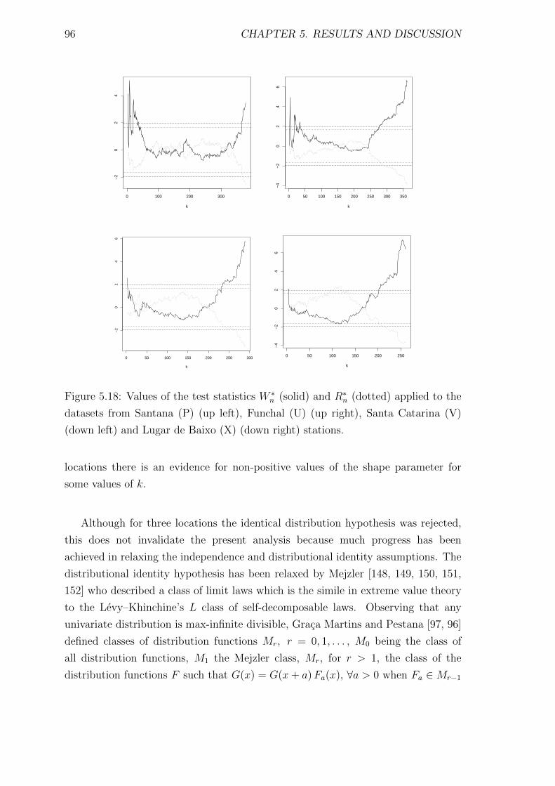
96 CHAPTER 5. RESULTS AND DISCUSSION
0 100 200 300
−2
02
4
k
0 50 100 150 200 250 300 350
−4
−2
02
46
k
0 50 100 150 200 250 300
−2
02
46
k
0 50 100 150 200 250
−4
−2
02
46
k
Figure 5.18: Values of the test statistics W ∗n (solid) and R∗n (dotted) applied to the
datasets from Santana (P) (up left), Funchal (U) (up right), Santa Catarina (V)
(down left) and Lugar de Baixo (X) (down right) stations.
locations there is an evidence for non-positive values of the shape parameter for
some values of k.
Although for three locations the identical distribution hypothesis was rejected,
this does not invalidate the present analysis because much progress has been
achieved in relaxing the independence and distributional identity assumptions. The
distributional identity hypothesis has been relaxed by Mejzler [148, 149, 150, 151,
152] who described a class of limit laws which is the simile in extreme value theory
to the Levy–Khinchine’s L class of self-decomposable laws. Observing that any
univariate distribution is max-infinite divisible, Graca Martins and Pestana [97, 96]
defined classes of distribution functions Mr, r = 0, 1, . . . , M0 being the class of
all distribution functions, M1 the Mejzler class, Mr, for r > 1, the class of the
distribution functions F such that G(x) = G(x+ a)Fa(x), ∀a > 0 when Fa ∈Mr−1

5.2. MONTHLY AND DAILY DATA – PORT AND POT APPROACHES 97
and M∞ =∞⋂r=0
Mr, where G = F if R is the support of the distribution function F ,
or a simple transformation whenever its support is a proper subset of the real line,
cf. Galambos [76]. Mejzler’s class can be characterised in terms of log-concavity
of G. Analogously, Graca Martins and Pestana Mr classes may be characterised
in terms of higher order monotonicity (fully described by Pestana and Mendonca
[170]) of the corresponding G, and M∞ in terms of complete monotonicity: F ∈M∞if and only the corresponding G satisfies G(x) = exp[−K(x)], with K completely
monotone. Hence, M∞ is a non-trivial extension of both the superclass of stable
extreme value distributions for maxima, and a subclass of Mejzler’s laws, that can
provide a proper framework to analyse maxima of linearly transformed data arising
from various parent distributions.
5.2.2 Threshold choice in a POT approach
The dataset analysed in this subsection, called Dataset IV, consists of daily
precipitation data provided by the Madeira Civil Engineering Laboratory’s
Department of Hydraulics and Energy Technologies from the stations whose
locations are shown in Figure 5.19.
Figure 5.19: Location and altitude range of the rain gauge stations–Dataset IV (Map
data c©2014 Google).
In the search for a threshold value for each one of these stations data, the
first step taken was to analyse each mean residual life plot. By way of example,
Figure 5.20 shows the obtained plots for Areeiro (A), Encumeada (E), Canhas (N)
and Funchal (U) stations belonging to the Classes 1, 2, 3 and 4, respectively.
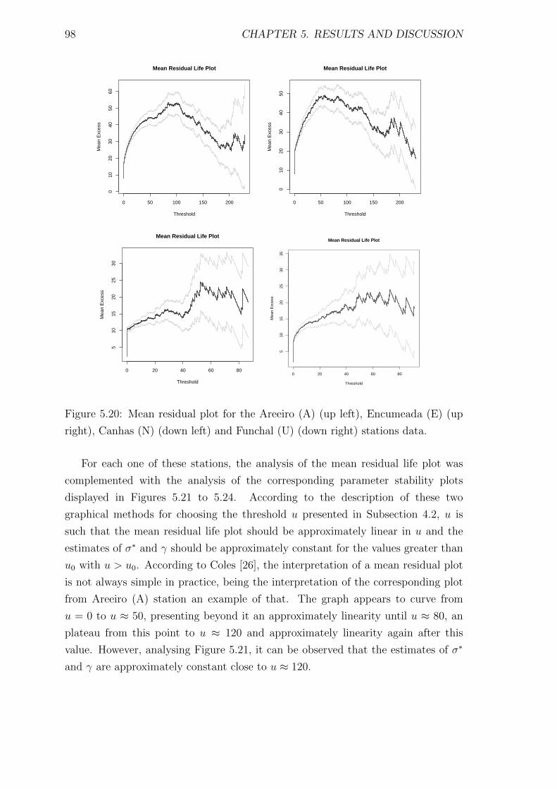
98 CHAPTER 5. RESULTS AND DISCUSSION
0 50 100 150 200
010
2030
4050
60
Mean Residual Life Plot
Threshold
Mea
n E
xces
s
0 50 100 150 200
010
2030
4050
Mean Residual Life Plot
Threshold
Mea
n E
xces
s
0 20 40 60 80
510
1520
2530
Mean Residual Life Plot
Threshold
Mea
n E
xces
s
0 20 40 60 80
510
1520
2530
35
Mean Residual Life Plot
Threshold
Mea
n E
xces
s
Figure 5.20: Mean residual plot for the Areeiro (A) (up left), Encumeada (E) (up
right), Canhas (N) (down left) and Funchal (U) (down right) stations data.
For each one of these stations, the analysis of the mean residual life plot was
complemented with the analysis of the corresponding parameter stability plots
displayed in Figures 5.21 to 5.24. According to the description of these two
graphical methods for choosing the threshold u presented in Subsection 4.2, u is
such that the mean residual life plot should be approximately linear in u and the
estimates of σ∗ and γ should be approximately constant for the values greater than
u0 with u > u0. According to Coles [26], the interpretation of a mean residual plot
is not always simple in practice, being the interpretation of the corresponding plot
from Areeiro (A) station an example of that. The graph appears to curve from
u = 0 to u ≈ 50, presenting beyond it an approximately linearity until u ≈ 80, an
plateau from this point to u ≈ 120 and approximately linearity again after this
value. However, analysing Figure 5.21, it can be observed that the estimates of σ∗
and γ are approximately constant close to u ≈ 120.
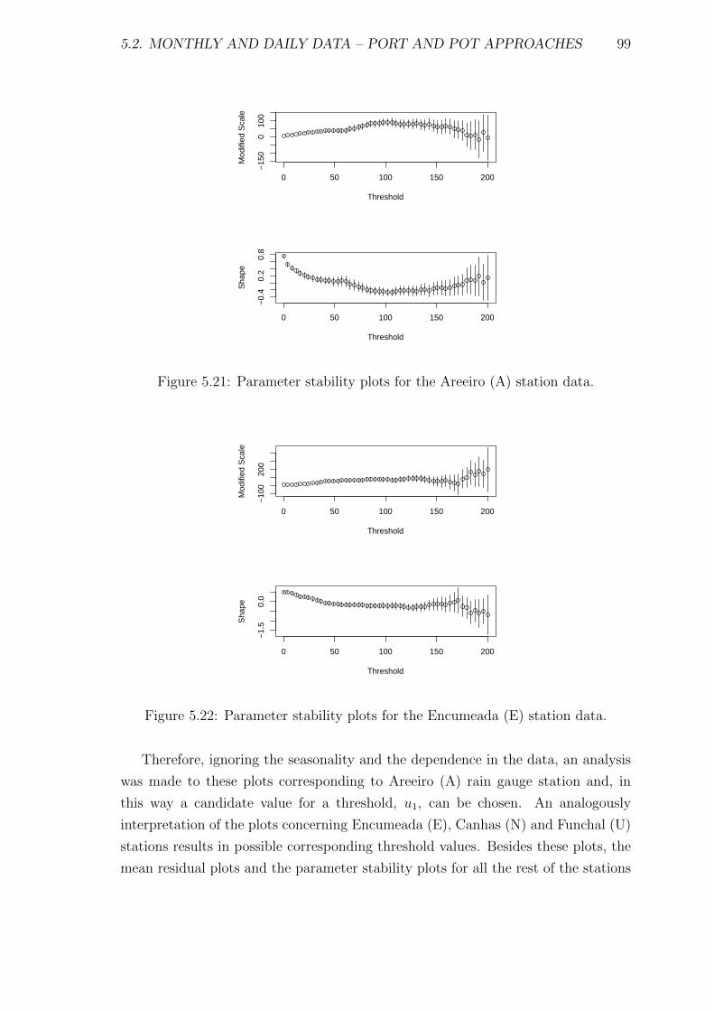
5.2. MONTHLY AND DAILY DATA – PORT AND POT APPROACHES 99
0 50 100 150 200
−15
00
100
Threshold
Mod
ified
Sca
le
0 50 100 150 200
−0.
40.
20.
8
Threshold
Sha
pe
Figure 5.21: Parameter stability plots for the Areeiro (A) station data.
0 50 100 150 200
−10
020
0
Threshold
Mod
ified
Sca
le
0 50 100 150 200
−1.
50.
0
Threshold
Sha
pe
Figure 5.22: Parameter stability plots for the Encumeada (E) station data.
Therefore, ignoring the seasonality and the dependence in the data, an analysis
was made to these plots corresponding to Areeiro (A) rain gauge station and, in
this way a candidate value for a threshold, u1, can be chosen. An analogously
interpretation of the plots concerning Encumeada (E), Canhas (N) and Funchal (U)
stations results in possible corresponding threshold values. Besides these plots, the
mean residual plots and the parameter stability plots for all the rest of the stations
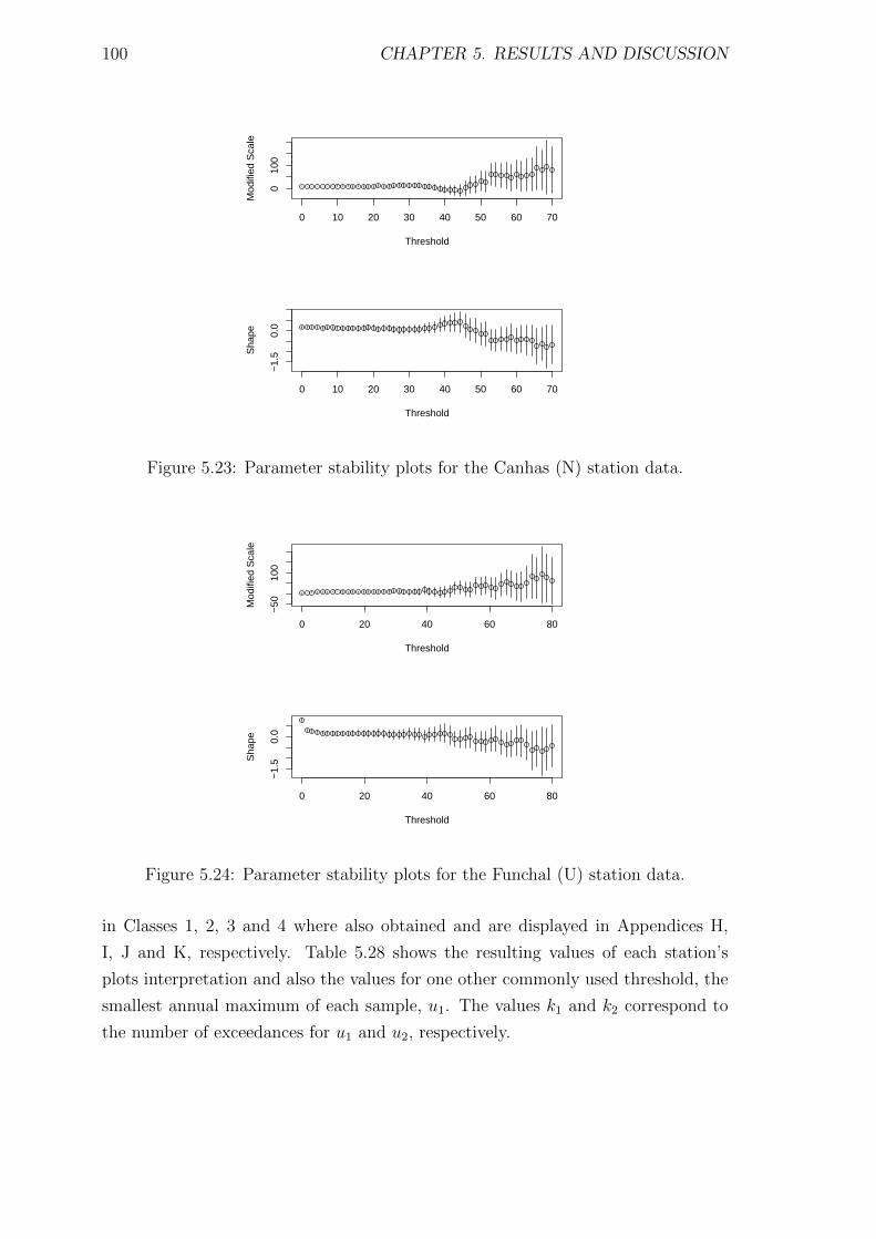
100 CHAPTER 5. RESULTS AND DISCUSSION
0 10 20 30 40 50 60 70
010
0
ThresholdM
odifi
ed S
cale
0 10 20 30 40 50 60 70
−1.
50.
0
Threshold
Sha
pe
Figure 5.23: Parameter stability plots for the Canhas (N) station data.
0 20 40 60 80
−50
100
Threshold
Mod
ified
Sca
le
0 20 40 60 80
−1.
50.
0
Threshold
Sha
pe
Figure 5.24: Parameter stability plots for the Funchal (U) station data.
in Classes 1, 2, 3 and 4 where also obtained and are displayed in Appendices H,
I, J and K, respectively. Table 5.28 shows the resulting values of each station’s
plots interpretation and also the values for one other commonly used threshold, the
smallest annual maximum of each sample, u1. The values k1 and k2 correspond to
the number of exceedances for u1 and u2, respectively.
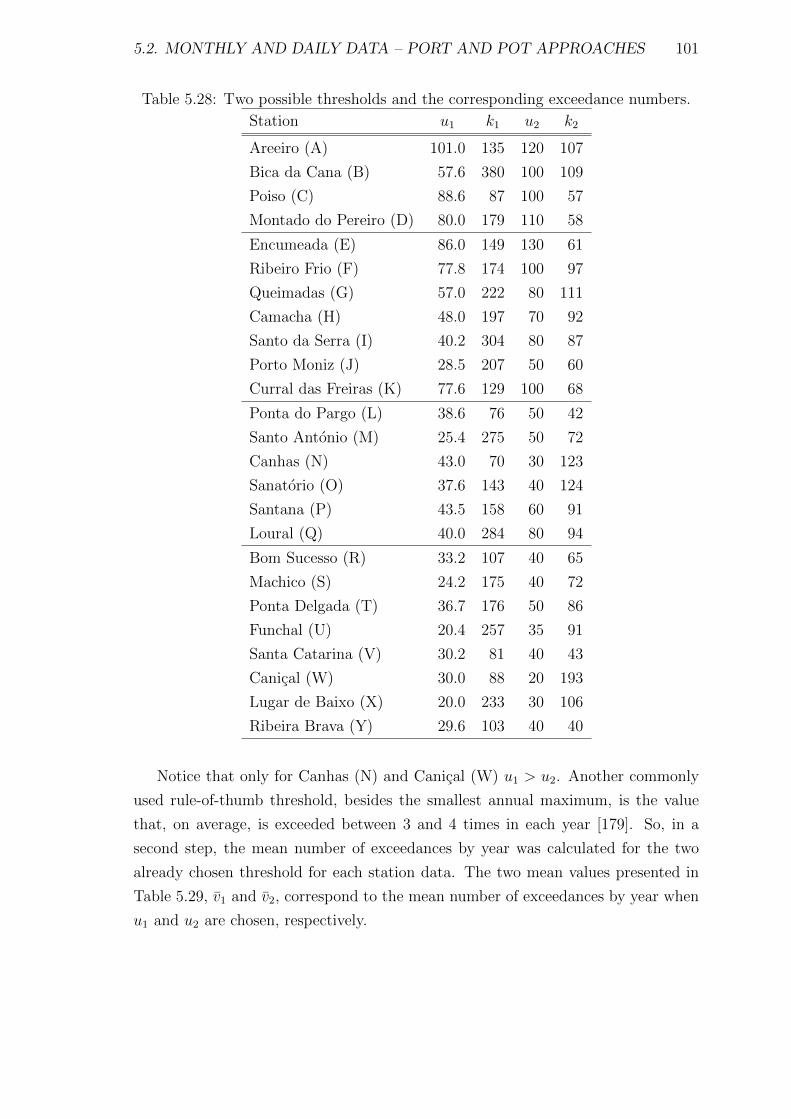
5.2. MONTHLY AND DAILY DATA – PORT AND POT APPROACHES 101
Table 5.28: Two possible thresholds and the corresponding exceedance numbers.
Station u1 k1 u2 k2
Areeiro (A) 101.0 135 120 107
Bica da Cana (B) 57.6 380 100 109
Poiso (C) 88.6 87 100 57
Montado do Pereiro (D) 80.0 179 110 58
Encumeada (E) 86.0 149 130 61
Ribeiro Frio (F) 77.8 174 100 97
Queimadas (G) 57.0 222 80 111
Camacha (H) 48.0 197 70 92
Santo da Serra (I) 40.2 304 80 87
Porto Moniz (J) 28.5 207 50 60
Curral das Freiras (K) 77.6 129 100 68
Ponta do Pargo (L) 38.6 76 50 42
Santo Antonio (M) 25.4 275 50 72
Canhas (N) 43.0 70 30 123
Sanatorio (O) 37.6 143 40 124
Santana (P) 43.5 158 60 91
Loural (Q) 40.0 284 80 94
Bom Sucesso (R) 33.2 107 40 65
Machico (S) 24.2 175 40 72
Ponta Delgada (T) 36.7 176 50 86
Funchal (U) 20.4 257 35 91
Santa Catarina (V) 30.2 81 40 43
Canical (W) 30.0 88 20 193
Lugar de Baixo (X) 20.0 233 30 106
Ribeira Brava (Y) 29.6 103 40 40
Notice that only for Canhas (N) and Canical (W) u1 > u2. Another commonly
used rule-of-thumb threshold, besides the smallest annual maximum, is the value
that, on average, is exceeded between 3 and 4 times in each year [179]. So, in a
second step, the mean number of exceedances by year was calculated for the two
already chosen threshold for each station data. The two mean values presented in
Table 5.29, v1 and v2, correspond to the mean number of exceedances by year when
u1 and u2 are chosen, respectively.
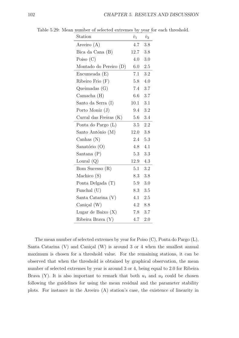
102 CHAPTER 5. RESULTS AND DISCUSSION
Table 5.29: Mean number of selected extremes by year for each threshold.
Station v1 v2
Areeiro (A) 4.7 3.8
Bica da Cana (B) 12.7 3.8
Poiso (C) 4.0 3.0
Montado do Pereiro (D) 6.0 2.5
Encumeada (E) 7.1 3.2
Ribeiro Frio (F) 5.8 4.0
Queimadas (G) 7.4 3.7
Camacha (H) 6.6 3.7
Santo da Serra (I) 10.1 3.1
Porto Moniz (J) 9.4 3.2
Curral das Freiras (K) 5.6 3.4
Ponta do Pargo (L) 3.5 2.2
Santo Antonio (M) 12.0 3.8
Canhas (N) 2.4 5.3
Sanatorio (O) 4.8 4.1
Santana (P) 5.3 3.3
Loural (Q) 12.9 4.3
Bom Sucesso (R) 5.1 3.2
Machico (S) 8.3 3.8
Ponta Delgada (T) 5.9 3.0
Funchal (U) 8.3 3.5
Santa Catarina (V) 4.1 2.5
Canical (W) 4.2 8.8
Lugar de Baixo (X) 7.8 3.7
Ribeira Brava (Y) 4.7 2.0
The mean number of selected extremes by year for Poiso (C), Ponta do Pargo (L),
Santa Catarina (V) and Canical (W) is around 3 or 4 when the smallest annual
maximum is chosen for a threshold value. For the remaining stations, it can be
observed that when the threshold is obtained by graphical observation, the mean
number of selected extremes by year is around 3 or 4, being equal to 2.0 for Ribeira
Brava (Y). It is also important to remark that both u1 and u2 could be chosen
following the guidelines for using the mean residual and the parameter stability
plots. For instance in the Areeiro (A) station’s case, the existence of linearity in
5.2. MONTHLY AND DAILY DATA – PORT AND POT APPROACHES 103
the mean residual plot (cf. Figure 5.20 on page 98) might be considered at the
right of both u1 = 101 and u2 = 120. Also, at these two values, the shape and
the modified scale parameters seem to be in a plateau (cf. Figure 5.21 on page 99)
comparing with other lower thresholds which can be considered to show bias–related
curvature. Like for Areeiro (A) station, it can be observed what it seems to be an
horizontal line for u1 and a down straight line for u2 in the mean residual plot of
Encumeada (E) station data (cf. Figure 5.20). These somehow similar diagnostic
plots for these two stations located in the interior of the island are quite different from
the ones corresponding to the two stations located nearest to the sea, Canhas (N) and
Funchal (U) (cf. Figure 5.20). For the station that belongs to Class 3, Canhas (N),
there are different plateaus in the parameter stability plots for u1 and u2, and what
it seems to be a down straight line for u1 and a upper straight line for u2 in the mean
residual plot. For the Funchal (U) station’s case, the shape and the modified scale
parameters seem to be in the same plateau for both u1 and u2, and an approximately
upper straight line before both u1 and u2 can be observed, but with wider intervals
for the latter value. The interpretation of these diagnostic plots is considered a
challenge with intrinsic subjectivity [26, 183], that often leads different threshold
choices resulting in diverse tail behaviours. Scarrot and MacDonald [183] suggest
an informal approach to this problem in which the sensitivity of the parameters and
return levels estimates to the different threshold choices are evaluated.
The violation of the independence and distributional equality assumptions may
also result into misleading diagnostic plots. The clustering of extreme values is
observed in many applications. Sometimes it is sufficient to consider the cluster
maxima, but other times the clusters time intervals and sizes of components
excesses need to be considered too [36]. Also, according to Engeland et al. [62] the
non-stationarity can, for instance, be accounted by subdividing the dataset into
blocks that are considered to be homogeneous or, in an alternative approach, by
letting the parameters in the GPD depend on time or on other covariates. The
present analysis is not complete, but is an important step in the analysis following
in what concerns non–stationarity. For the first approach to non–stationarity,
the obtained results indicate that caution is needed when dividing each of the
stations datasets. Indeed, the exceedances percentage by month for the both
chosen thresholds displayed in Appendix L reveal that seasonality might not be
the same for all locations. Although for all the stations with the exception of
Bom Sucesso (R), the highest percentages belong to the rainy season (October to
March), the difference is not so pronounced between some of these percentages and
104 CHAPTER 5. RESULTS AND DISCUSSION
the ones presented by others months like April or September for a few stations.
These sample percentages support the observation made by Lang et al. [134] that
the advantages of a seasonal approach may be lost when the division of the year
into alleged homogeneous seasons is somehow slightly unreal. The second approach
to non–stationarity mentioned by Engeland et al. [62] was applied, for example,
in the papers by Smith [196] and Katz et al. [124], but unlike Katz et al. [124],
Smith [196] does not assume any specific form of seasonal variation. On the other
hand, Katz et al. [124] do not apply an initial declustering process. Indirectly using
the POT approach, Katz et al. [124] fit to a time series of daily precipitation the
GEV distribution that is fitted to the annual maxima by ML, assuming that these
values of daily precipitation amount have a GEV distribution with parameters that
can be written through sine waves depending on the day t within a given year. The
application of the two mentioned approaches to non-stationarity to the Dataset IV,
and the consequent comparison of results in terms of parameters and return levels
estimates is postponed for future work.
5.3 Spatial annual maxima – Copula functions
A variety of statistical tools, such as copulas and spatial max-stable processes,
have been used in the most recent decades for modelling spatial extreme data. A
review of spatial extremes methods based on latent variables, copulas and spatial
max-stable processes is presented by Davison et al. [37], who refer that appropriately
chosen copula or max-stable models seem to be essential for the modelling of spatial
extremes. The importance of max-stable processes and copula approaches for
modelling spatial dependence is also emphasised by other authors such as Cooley et
al. [31]. Although most of the studies on spatial extremes mentioned in the reviews
cited above focus on modelling block maxima data, it is important to mention
here that there are other studies (e.g., [185]) where these same methods are also
applied to continuous time series of daily aggregated precipitation. The dependence
between variables plays a central role in multivariate extremes. The ability to
describe and model the dependence between variables, regardless of their marginal
distribution functions, is the major advantage of the copula functions approach. In
practice, the application of these functions to the data can be considered based on
an estimate of a measure of association, for example, the Kendall’s τ [156, 182].
In order to quantify this association in the case of Madeira island’s extreme
rainfall, an estimate for the Kendall’s τ value is calculated, using the annual maxima
5.3. SPATIAL ANNUAL MAXIMA – COPULA FUNCTIONS 105
data from rain gauge stations maintained in the past by the General Council of
the Autonomous District of Funchal. Thus, for each pair (X, Y ), where X and Y
correspond to the maxima annual dataset obtained in the stations identified by the
same letters, the independence was analysed through the application of a test based
on the empirical version of Kendall’s τ association measure [81]. In a second stage
of the study, groups of three stations, with the ones for which the independence was
rejected at the significance level of α = 0.01. Then, the estimated values of Kendall’s
τ measure of association from each pair were used to determine the coefficients of
the extreme value copula C defined by (4.31) in Section 4.3 of the Methodology.
Since the regarded stations do not have the same measurement period, the maxima
annual datasets were divided into three subsets according to the different periods.
The highest values of annual daily precipitation on the island of Madeira, in the
period of 1950–1980, that will be termed by Dataset V, come from 12 stations,
namely, Areeiro (A), Bica da Cana (B), Montado do Pereiro (D), Ribeiro Frio (F),
Queimadas (G), Camacha (H), Santo da Serra (I), Sanatorio (O), Santana (P),
Ponta Delgada (T), Funchal (U) and Lugar de Baixo (X) stations. Dataset VI
corresponds to the shorter period 1950–1972 and includes Porto Moniz (J), Curral
das Freiras (K), Ponta do Pargo (L), Santo Antonio (M), Canhas (N), Loural(Q)
and Ribeira Brava (Y) stations. Finally, Dataset VII will consist of the 12 stations
of the Dataset V and Poiso (C), Encumeada (E), Bom Sucesso (R), Machico (S),
Santa Catarina (V) and Canical (W) stations. Besides the better coverage of
Madeira Island naturally obtained by an increase of the number of rain gauge
stations, Datasets VI and VII add information to the study because two regions of
the island not considered in the analysis made with Dataset V are included. More
precisely, with the data from Porto Moniz (J) and Ponta do Pargo (L) stations the
region further west of the island is included in the study performed with Dataset VI,
while the region further east is covered when the data coming from Machico (S),
Santa Catarina (V) and Canical (W) stations included in Dataset VII is considered.
The analysis corresponding to Dataset V led to 17 groups of three pairwise
associated stations, while the analysis made to Datasets VI and VII originated 40
and 16 groups, respectively. These differences between the studies of Datasets V,
VI and VII visible in terms of number of groups are even more pronounced since
there is no group common to these three analysis among the ones formed by three
stations with measurement period ranging from 1950 to 1980. For the period 1950–
1972, 34 of the groups include one or more rain gauge stations of the seven extra
stations considered relatively to the wider period, being the remaining six groups
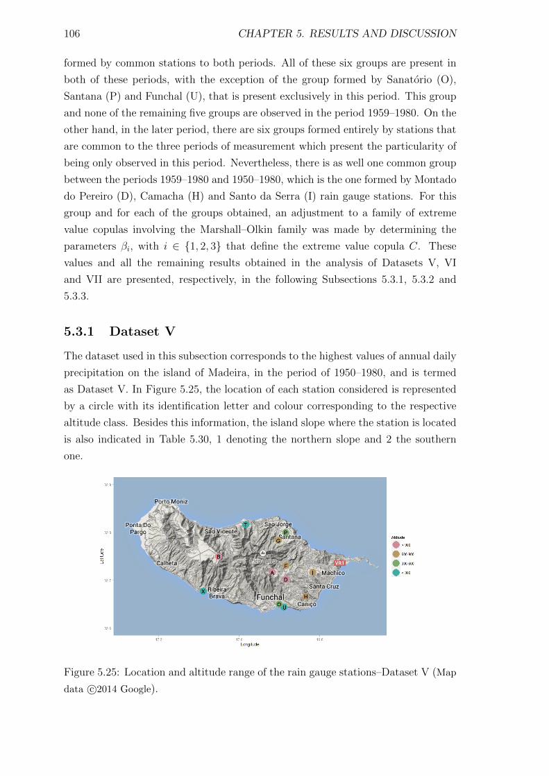
106 CHAPTER 5. RESULTS AND DISCUSSION
formed by common stations to both periods. All of these six groups are present in
both of these periods, with the exception of the group formed by Sanatorio (O),
Santana (P) and Funchal (U), that is present exclusively in this period. This group
and none of the remaining five groups are observed in the period 1959–1980. On the
other hand, in the later period, there are six groups formed entirely by stations that
are common to the three periods of measurement which present the particularity of
being only observed in this period. Nevertheless, there is as well one common group
between the periods 1959–1980 and 1950–1980, which is the one formed by Montado
do Pereiro (D), Camacha (H) and Santo da Serra (I) rain gauge stations. For this
group and for each of the groups obtained, an adjustment to a family of extreme
value copulas involving the Marshall–Olkin family was made by determining the
parameters βi, with i ∈ {1, 2, 3} that define the extreme value copula C. These
values and all the remaining results obtained in the analysis of Datasets V, VI
and VII are presented, respectively, in the following Subsections 5.3.1, 5.3.2 and
5.3.3.
5.3.1 Dataset V
The dataset used in this subsection corresponds to the highest values of annual daily
precipitation on the island of Madeira, in the period of 1950–1980, and is termed
as Dataset V. In Figure 5.25, the location of each station considered is represented
by a circle with its identification letter and colour corresponding to the respective
altitude class. Besides this information, the island slope where the station is located
is also indicated in Table 5.30, 1 denoting the northern slope and 2 the southern
one.
Figure 5.25: Location and altitude range of the rain gauge stations–Dataset V (Map
data c©2014 Google).
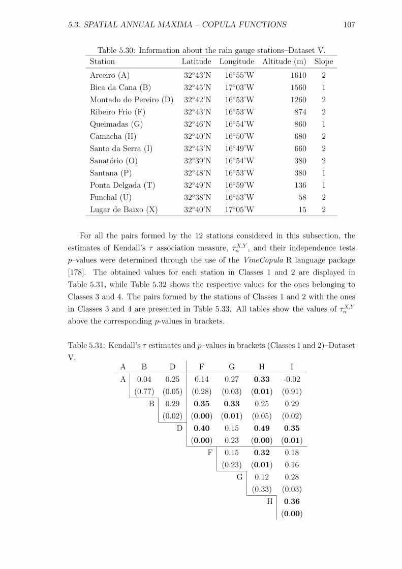
5.3. SPATIAL ANNUAL MAXIMA – COPULA FUNCTIONS 107
Table 5.30: Information about the rain gauge stations–Dataset V.
Station Latitude Longitude Altitude (m) Slope
Areeiro (A) 32◦43’N 16◦55’W 1610 2
Bica da Cana (B) 32◦45’N 17◦03’W 1560 1
Montado do Pereiro (D) 32◦42’N 16◦53’W 1260 2
Ribeiro Frio (F) 32◦43’N 16◦53’W 874 2
Queimadas (G) 32◦46’N 16◦54’W 860 1
Camacha (H) 32◦40’N 16◦50’W 680 2
Santo da Serra (I) 32◦43’N 16◦49’W 660 2
Sanatorio (O) 32◦39’N 16◦54’W 380 2
Santana (P) 32◦48’N 16◦53’W 380 1
Ponta Delgada (T) 32◦49’N 16◦59’W 136 1
Funchal (U) 32◦38’N 16◦53’W 58 2
Lugar de Baixo (X) 32◦40’N 17◦05’W 15 2
For all the pairs formed by the 12 stations considered in this subsection, the
estimates of Kendall’s τ association measure, τX,Yn , and their independence tests
p–values were determined through the use of the VineCopula R language package
[178]. The obtained values for each station in Classes 1 and 2 are displayed in
Table 5.31, while Table 5.32 shows the respective values for the ones belonging to
Classes 3 and 4. The pairs formed by the stations of Classes 1 and 2 with the ones
in Classes 3 and 4 are presented in Table 5.33. All tables show the values of τX,Yn
above the corresponding p-values in brackets.
Table 5.31: Kendall’s τ estimates and p–values in brackets (Classes 1 and 2)–Dataset
V.A B D F G H I
A 0.04 0.25 0.14 0.27 0.33 -0.02
(0.77) (0.05) (0.28) (0.03) (0.01) (0.91)
B 0.29 0.35 0.33 0.25 0.29
(0.02) (0.00) (0.01) (0.05) (0.02)
D 0.40 0.15 0.49 0.35
(0.00) 0.23 (0.00) (0.01)
F 0.15 0.32 0.18
(0.23) (0.01) 0.16
G 0.12 0.28
(0.33) (0.03)
H 0.36
(0.00)
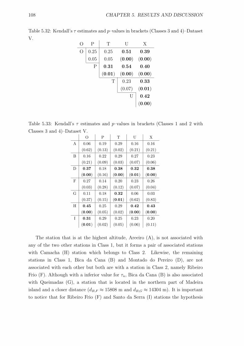
108 CHAPTER 5. RESULTS AND DISCUSSION
Table 5.32: Kendall’s τ estimates and p–values in brackets (Classes 3 and 4)–Dataset
V.O P T U X
O 0.25 0.25 0.51 0.39
0.05 0.05 (0.00) (0.00)
P 0.31 0.54 0.40
(0.01) (0.00) (0.00)
T 0.23 0.33
(0.07) (0.01)
U 0.42
(0.00)
Table 5.33: Kendall’s τ estimates and p–values in brackets (Classes 1 and 2 with
Classes 3 and 4)–Dataset V.O P T U X
A 0.06 0.19 0.29 0.16 0.16
(0.62) (0.13) (0.02) (0.21) (0.21)
B 0.16 0.22 0.29 0.27 0.23
(0.21) (0.09) (0.03) (0.07) (0.06)
D 0.37 0.18 0.38 0.32 0.38
(0.00) (0.16) (0.00) (0.01) (0.00)
F 0.27 0.14 0.20 0.23 0.26
(0.03) (0.28) (0.12) (0.07) (0.04)
G 0.11 0.18 0.32 0.06 0.03
(0.37) (0.15) (0.01) (0.62) (0.83)
H 0.45 0.25 0.29 0.42 0.43
(0.00) (0.05) (0.02) (0.00) (0.00)
I 0.31 0.29 0.25 0.23 0.20
(0.01) (0.02) (0.05) (0.06) (0.11)
The station that is at the highest altitude, Areeiro (A), is not associated with
any of the two other stations in Class 1, but it forms a pair of associated stations
with Camacha (H) station which belongs to Class 2. Likewise, the remaining
stations in Class 1, Bica da Cana (B) and Montado do Pereiro (D), are not
associated with each other but both are with a station in Class 2, namely Ribeiro
Frio (F). Although with a inferior value for τn, Bica da Cana (B) is also associated
with Queimadas (G), a station that is located in the northern part of Madeira
island and a closer distance (dB,F ≈ 15808 m and dB,G ≈ 14304 m). It is important
to notice that for Ribeiro Frio (F) and Santo da Serra (I) stations the hypothesis
5.3. SPATIAL ANNUAL MAXIMA – COPULA FUNCTIONS 109
of independence of the corresponding data sets is not rejected at a 0.01 significance
level although the proximity between these two stations (dI,F ≈ 6421 m) is smaller
than the one between the associated Santo da Serra (I) and Santana (P) stations
(dI,P ≈ 11158 m). The hypothesis of independence is also not rejected for the
even closer stations Santana (P) and Queimadas (G) (dG,P ≈ 2615 m), that are
both located in the northern part of the island. Santana (P) station forms with
Funchal (U) station the pair that presents the higher Kendall’s τ empirical value.
Despite their proximity to the sea, Santana (P) and Funchal (U) are located in
different slopes and the distance between them is higher than the one between
Santana (P) and Ponta Delgada (T) stations that present a much smaller value
of τn (τP,Tn = 0.31). This value is even smaller than the ones presented by the
pairs formed by these stations and another station closer to the sea but in the
opposite slope, namely Lugar de Baixo (X). Besides this group of three stations,
Santana (P) forms with Funchal (U) and Lugar de Baixo (X) another group of
pairwise associated stations formed by a station in Class 3 and two others in Class
4. The second highest estimate for Kendall’s τ is presented by the pair formed
by Sanatorio (O) and Funchal (U) stations (τO,Un = 0.51), that are located in
different altitudes but very close to each other (dO,U = 1328 m). These two stations
also show a statistically significant concordance with Lugar de Baixo (X) station,
forming a group of pairwise associated stations located near the sea. Sanatorio (O),
Funchal (U) and Lugar de Baixo (X) stations are all in association with Montado
do Pereiro (D) and Camacha (H) stations, which belong to different classes of
altitude and are located farther way of the sea. These two stations form the pair of
associated stations with the third highest value for τn observed in Dataset V, being
both also associated with Ribeiro Frio (F) and Santo da Serra (I) stations.
In short, Tables 5.34 and 5.35 show all the groups formed by three pairwise
associated stations (s1 − s2 − s3), the corresponding parameters βi of the extreme
value copula C defined by (4.31) in Section 4.3 of the Methodology, and the distances
between stations within each group ((d1,2, d1,3, d2,3), where di,j stands for the distance
in m between stations si and sj – cf. Tables 3.1–3.3). Table 5.34 shows all the
groups including Montado do Pereiro (D) (set 1), being the remaining groups (set 2)
displayed in Table 5.35. All the results presented were obtained using functions that
were implemented in R, whose corresponding code is presented in Appendix M.
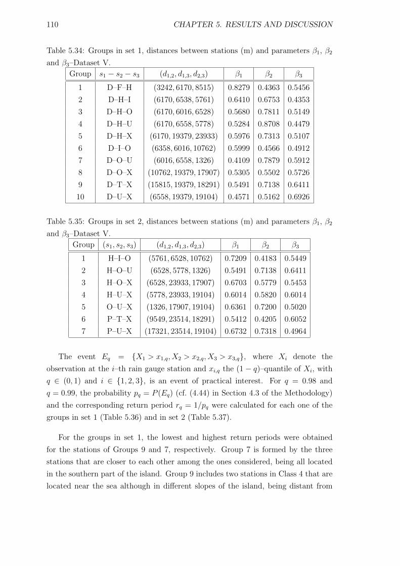
110 CHAPTER 5. RESULTS AND DISCUSSION
Table 5.34: Groups in set 1, distances between stations (m) and parameters β1, β2
and β3–Dataset V.
Group s1 − s2 − s3 (d1,2, d1,3, d2,3) β1 β2 β3
1 D–F–H (3242, 6170, 8515) 0.8279 0.4363 0.5456
2 D–H–I (6170, 6538, 5761) 0.6410 0.6753 0.4353
3 D–H–O (6170, 6016, 6528) 0.5680 0.7811 0.5149
4 D–H–U (6170, 6558, 5778) 0.5284 0.8708 0.4479
5 D–H–X (6170, 19379, 23933) 0.5976 0.7313 0.5107
6 D–I–O (6358, 6016, 10762) 0.5999 0.4566 0.4912
7 D–O–U (6016, 6558, 1326) 0.4109 0.7879 0.5912
8 D–O–X (10762, 19379, 17907) 0.5305 0.5502 0.5726
9 D–T–X (15815, 19379, 18291) 0.5491 0.7138 0.6411
10 D–U–X (6558, 19379, 19104) 0.4571 0.5162 0.6926
Table 5.35: Groups in set 2, distances between stations (m) and parameters β1, β2
and β3–Dataset V.
Group (s1, s2, s3) (d1,2, d1,3, d2,3) β1 β2 β3
1 H–I–O (5761, 6528, 10762) 0.7209 0.4183 0.5449
2 H–O–U (6528, 5778, 1326) 0.5491 0.7138 0.6411
3 H–O–X (6528, 23933, 17907) 0.6703 0.5779 0.5453
4 H–U–X (5778, 23933, 19104) 0.6014 0.5820 0.6014
5 O–U–X (1326, 17907, 19104) 0.6361 0.7200 0.5020
6 P–T–X (9549, 23514, 18291) 0.5412 0.4205 0.6052
7 P–U–X (17321, 23514, 19104) 0.6732 0.7318 0.4964
The event Eq = {X1 > x1,q, X2 > x2,q, X3 > x3,q}, where Xi denote the
observation at the i–th rain gauge station and xi,q the (1− q)–quantile of Xi, with
q ∈ (0, 1) and i ∈ {1, 2, 3}, is an event of practical interest. For q = 0.98 and
q = 0.99, the probability pq = P (Eq) (cf. (4.44) in Section 4.3 of the Methodology)
and the corresponding return period rq = 1/pq were calculated for each one of the
groups in set 1 (Table 5.36) and in set 2 (Table 5.37).
For the groups in set 1, the lowest and highest return periods were obtained
for the stations of Groups 9 and 7, respectively. Group 7 is formed by the three
stations that are closer to each other among the ones considered, being all located
in the southern part of the island. Group 9 includes two stations in Class 4 that are
located near the sea although in different slopes of the island, being distant from
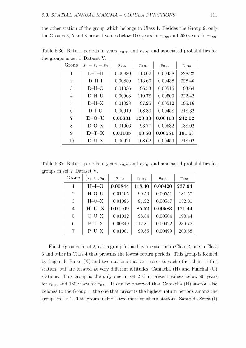
5.3. SPATIAL ANNUAL MAXIMA – COPULA FUNCTIONS 111
the other station of the group which belongs to Class 1. Besides the Group 9, only
the Groups 3, 5 and 8 present values below 100 years for r0.98 and 200 years for r0.99.
Table 5.36: Return periods in years, r0.98 and r0.99, and associated probabilities for
the groups in set 1–Dataset V.
Group s1 − s2 − s3 p0.98 r0.98 p0.99 r0.99
1 D–F–H 0.00880 113.62 0.00438 228.22
2 D–H–I 0.00880 113.60 0.00438 228.46
3 D–H–O 0.01036 96.53 0.00516 193.64
4 D–H–U 0.00903 110.78 0.00500 222.42
5 D–H–X 0.01028 97.25 0.00512 195.16
6 D–I–O 0.00919 108.80 0.00458 218.32
7 D–O–U 0.00831 120.33 0.00413 242.02
8 D–O–X 0.01066 93.77 0.00532 188.02
9 D–T–X 0.01105 90.50 0.00551 181.57
10 D–U–X 0.00921 108.62 0.00459 218.02
Table 5.37: Return periods in years, r0.98 and r0.99, and associated probabilities for
groups in set 2–Dataset V.
Group (s1, s2, s3) p0.98 r0.98 p0.99 r0.99
1 H–I–O 0.00844 118.40 0.00420 237.94
2 H–O–U 0.01105 90.50 0.00551 181.57
3 H–O–X 0.01096 91.22 0.00547 182.91
4 H–U–X 0.01169 85.52 0.00583 171.44
5 O–U–X 0.01012 98.84 0.00504 198.44
6 P–T–X 0.00849 117.81 0.00422 236.72
7 P–U–X 0.01001 99.85 0.00499 200.58
For the groups in set 2, it is a group formed by one station in Class 2, one in Class
3 and other in Class 4 that presents the lowest return periods. This group is formed
by Lugar de Baixo (X) and two stations that are closer to each other than to this
station, but are located at very different altitudes, Camacha (H) and Funchal (U)
stations. This group is the only one in set 2 that present values below 90 years
for r0.98 and 180 years for r0.99. It can be observed that Camacha (H) station also
belongs to the Group 1, the one that presents the highest return periods among the
groups in set 2. This group includes two more southern stations, Santo da Serra (I)
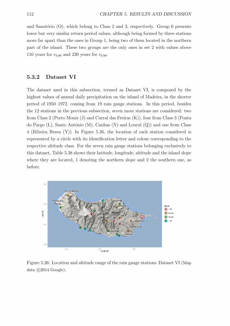
112 CHAPTER 5. RESULTS AND DISCUSSION
and Sanatorio (O), which belong to Class 2 and 3, respectively. Group 6 presents
lower but very similar return period values, although being formed by three stations
more far apart than the ones in Group 1, being two of them located in the northern
part of the island. These two groups are the only ones in set 2 with values above
110 years for r0.98 and 230 years for r0.99.
5.3.2 Dataset VI
The dataset used in this subsection, termed as Dataset VI, is composed by the
highest values of annual daily precipitation on the island of Madeira, in the shorter
period of 1950–1972, coming from 19 rain gauge stations. In this period, besides
the 12 stations in the previous subsection, seven more stations are considered: two
from Class 2 (Porto Moniz (J) and Curral das Freiras (K)), four from Class 3 (Ponta
do Pargo (L), Santo Antonio (M), Canhas (N) and Loural (Q)) and one from Class
4 (Ribeira Brava (Y)). In Figure 5.26, the location of each station considered is
represented by a circle with its identification letter and colour corresponding to the
respective altitude class. For the seven rain gauge stations belonging exclusively to
this dataset, Table 5.38 shows their latitude, longitude, altitude and the island slope
where they are located, 1 denoting the northern slope and 2 the southern one, as
before.
Figure 5.26: Location and altitude range of the rain gauge stations–Dataset VI (Map
data c©2014 Google).

5.3. SPATIAL ANNUAL MAXIMA – COPULA FUNCTIONS 113
Table 5.38: Information about the seven rain gauge stations belonging exclusively
to Dataset VI.Station Latitude Longitude Altitude (m) Slope
Porto Moniz (J) 32◦50’N 17◦11’W 653 1
Curral das Freiras (K) 32◦43’N 16◦58’W 650 2
Ponta do Pargo (L) 32◦47’N 17◦14’W 570 2
Santo Antonio (M) 32◦40’N 16◦57’W 525 2
Canhas (N) 32◦41’N 17◦07’W 425 2
Loural (Q) 32◦46’N 17◦02’W 307 1
Ribeira Brava (Y) 32◦40’N 17◦04’W 10 2
As in the previous subsection, for all pairs formed by the stations considered in
this subsection, the values of the Kendall’s τ association measure, τX,Yn , and their
independence tests p-values were determined through the use of the VineCopula R
language package [178]. The obtained values for each station in Classes 1 and 2 are
displayed in Table 5.39, while Table 5.40 shows the values for the ones that are in
Classes 3 and 4. The pairs formed by the stations of Classes 1 and 2 with the ones
in Classes 3 and 4 are presented in Table 5.41. All tables show the values of τX,Yn
above the corresponding p-values in brackets.
In the following analysis, the identification of the dataset considered will be added
as a subscript when a comparison between obtained values in different datasets shows
itself to be relevant. For example, τX,Yn,V I will refer to the estimate of the Kendall’s τ
association between stations X and Y when considering Dataset VI. Despite the high
distance between them (dJ,K ≈ 25618 m), Porto Moniz (J) station is only associated
with one other station that belongs to the same class of altitude, namely Curral
das Freiras (K) station. The latter one is also associated with Bica da Cana (B),
a nearest station located in Madeira island’s orographic barrier, but at a higher
altitude. Like in the period analysed in the previous subsection, there is here also a
statistically significant association between Bica da Cana (B) and Ribeiro Frio (F)
although with a higher value for the empirical version of the Kendall’s τ association
measure (τB,Fn,V = 0.35 and τB,Fn,V I = 0.48). Conversely, Montado do Pereiro (D)
and Camacha (H) stations form a pair of associated stations that present a lower
estimate of τn when the shorter period is considered (τD,Hn,V = 0.49 and τD,Hn,V I = 0.45).
The stations in this pair are also associated with Sanatorio (O) and Funchal (U)
stations in Class 4 likewise as in the period 1950–1980, presenting other associations
with two stations only considered in this period, namely Santo Antonio (M) and
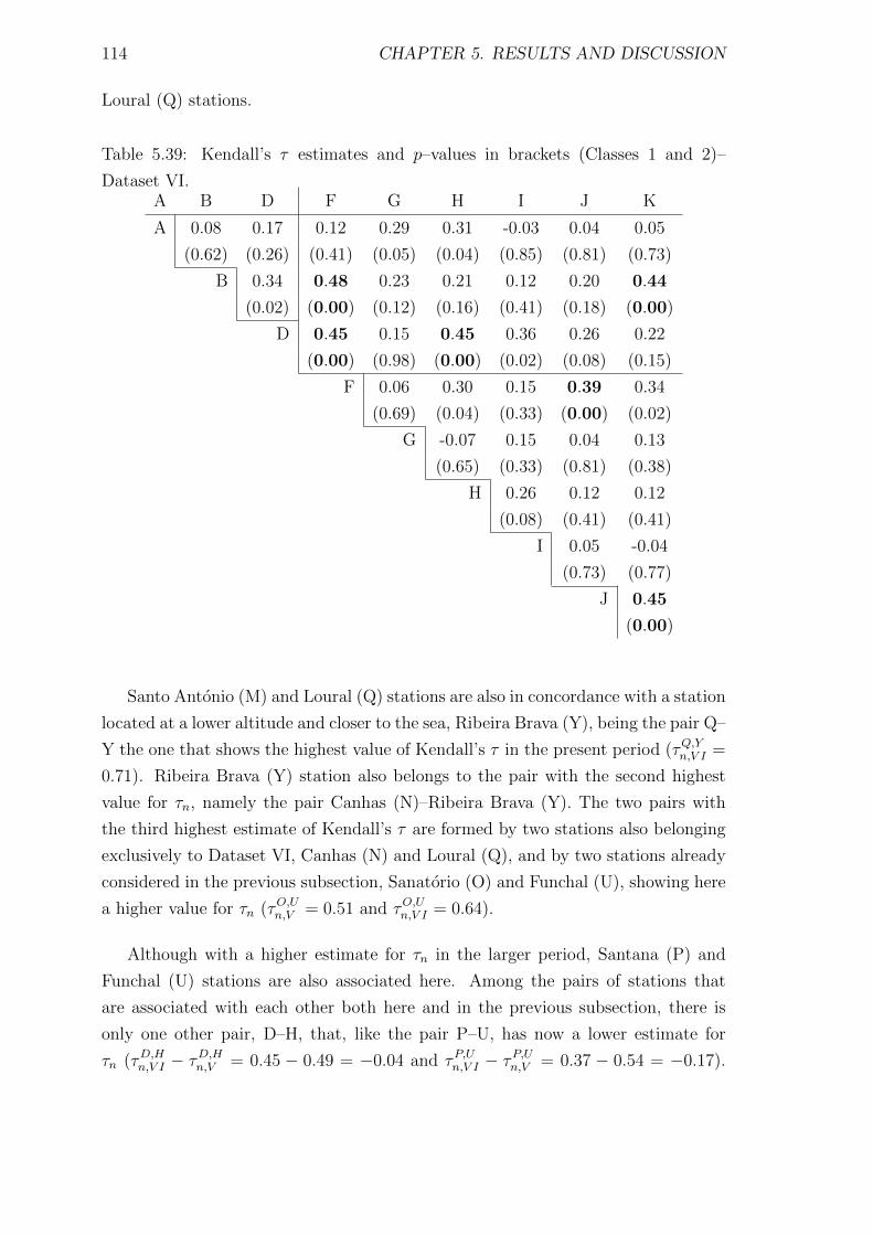
114 CHAPTER 5. RESULTS AND DISCUSSION
Loural (Q) stations.
Table 5.39: Kendall’s τ estimates and p–values in brackets (Classes 1 and 2)–
Dataset VI.A B D F G H I J K
A 0.08 0.17 0.12 0.29 0.31 -0.03 0.04 0.05
(0.62) (0.26) (0.41) (0.05) (0.04) (0.85) (0.81) (0.73)
B 0.34 0.48 0.23 0.21 0.12 0.20 0.44
(0.02) (0.00) (0.12) (0.16) (0.41) (0.18) (0.00)
D 0.45 0.15 0.45 0.36 0.26 0.22
(0.00) (0.98) (0.00) (0.02) (0.08) (0.15)
F 0.06 0.30 0.15 0.39 0.34
(0.69) (0.04) (0.33) (0.00) (0.02)
G -0.07 0.15 0.04 0.13
(0.65) (0.33) (0.81) (0.38)
H 0.26 0.12 0.12
(0.08) (0.41) (0.41)
I 0.05 -0.04
(0.73) (0.77)
J 0.45
(0.00)
Santo Antonio (M) and Loural (Q) stations are also in concordance with a station
located at a lower altitude and closer to the sea, Ribeira Brava (Y), being the pair Q–
Y the one that shows the highest value of Kendall’s τ in the present period (τQ,Yn,V I =
0.71). Ribeira Brava (Y) station also belongs to the pair with the second highest
value for τn, namely the pair Canhas (N)–Ribeira Brava (Y). The two pairs with
the third highest estimate of Kendall’s τ are formed by two stations also belonging
exclusively to Dataset VI, Canhas (N) and Loural (Q), and by two stations already
considered in the previous subsection, Sanatorio (O) and Funchal (U), showing here
a higher value for τn (τO,Un,V = 0.51 and τO,Un,V I = 0.64).
Although with a higher estimate for τn in the larger period, Santana (P) and
Funchal (U) stations are also associated here. Among the pairs of stations that
are associated with each other both here and in the previous subsection, there is
only one other pair, D–H, that, like the pair P–U, has now a lower estimate for
τn (τD,Hn,V I − τD,Hn,V = 0.45 − 0.49 = −0.04 and τP,Un,V I − τ
P,Un,V = 0.37 − 0.54 = −0.17).
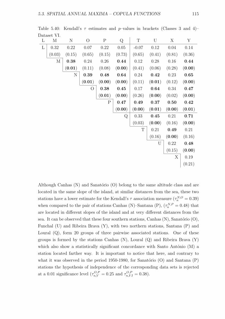
5.3. SPATIAL ANNUAL MAXIMA – COPULA FUNCTIONS 115
Table 5.40: Kendall’s τ estimates and p–values in brackets (Classes 3 and 4)–
Dataset VI.L M N O P Q T U X Y
L 0.32 0.22 0.07 0.22 0.05 -0.07 0.12 0.04 0.14
(0.03) (0.15) (0.65) (0.15) (0.73) (0.65) (0.41) (0.81) (0.36)
M 0.38 0.24 0.26 0.44 0.12 0.28 0.16 0.44
(0.01) (0.11) (0.08) (0.00) (0.41) (0.06) (0.28) (0.00)
N 0.39 0.48 0.64 0.24 0.42 0.23 0.65
(0.01) (0.00) (0.00) (0.11) (0.01) (0.12) (0.00)
O 0.38 0.45 0.17 0.64 0.34 0.47
(0.01) (0.00) (0.26) (0.00) (0.02) (0.00)
P 0.47 0.49 0.37 0.50 0.42
(0.00) (0.00) (0.01) (0.00) (0.01)
Q 0.33 0.45 0.21 0.71
(0.03) (0.00) (0.16) (0.00)
T 0.21 0.49 0.21
(0.16) (0.00) (0.16)
U 0.22 0.48
(0.15) (0.00)
X 0.19
(0.21)
Although Canhas (N) and Sanatorio (O) belong to the same altitude class and are
located in the same slope of the island, at similar distances from the sea, these two
stations have a lower estimate for the Kendall’s τ association measure (τN,On = 0.39)
when compared to the pair of stations Canhas (N)–Santana (P), (τN,Pn = 0.48) that
are located in different slopes of the island and at very different distances from the
sea. It can be observed that these four southern stations, Canhas (N), Sanatorio (O),
Funchal (U) and Ribeira Brava (Y), with two northern stations, Santana (P) and
Loural (Q), form 20 groups of three pairwise associated stations. One of these
groups is formed by the stations Canhas (N), Loural (Q) and Ribeira Brava (Y)
which also show a statistically significant concordance with Santo Antonio (M) a
station located farther way. It is important to notice that here, and contrary to
what it was observed in the period 1950-1980, for Sanatorio (O) and Santana (P)
stations the hypothesis of independence of the corresponding data sets is rejected
at a 0.01 significance level (τO,Pn,V = 0.25 and τO,Pn,V I = 0.38).

116 CHAPTER 5. RESULTS AND DISCUSSION
Table 5.41: Kendall’s τ estimates and p–values in brackets (Classes 1 and 2 with
Classes 3 and 4)–Dataset VI.L M N O P Q T U X Y
A 0.03 0.31 0.02 0.04 0.15 0.09 0.23 0.05 0.30 0.04
(0.85) (0.04) (0.89) (0.77) (0.32) (0.54) (0.13) (0.73) (0.05) (0.81)
B 0.10 0.37 0.22 0.08 0.22 0.32 0.28 0.22 0.08 0.23
(0.51) (0.01) (0.15) (0.58) (0.15) (0.03) (0.06) (0.15) (0.58) (0.12)
D 0.19 0.49 0.25 0.38 0.28 0.45 0.22 0.44 0.15 0.36
(0.20) (0.00) (0.10) (0.01) (0.06) (0.00) (0.15) (0.00) (0.33) (0.02)
F 0.19 0.35 0.09 0.29 0.20 0.21 0.11 0.26 0.21 0.11
(0.20) (0.02) (0.54) (0.05) (0.18) (0.16) (0.48) (0.08) (0.16) (0.48)
G 0.09 0.09 0.07 -0.02 0.23 -0.05 0.26 -0.04 0.38 0.08
(0.54) (0.54) (0.65) (0.89) (0.13) (0.73) (0.09) (0.77) (0.01) (0.58)
H 0.18 0.53 0.31 0.48 0.30 0.45 0.14 0.45 0.27 0.39
(0.23) (0.00) (0.04) (0.00) (0.05) (0.00) (0.36) (0.00) (0.07) (0.01)
I 0.30 0.34 0.26 0.31 0.43 0.28 0.19 0.29 0.12 0.34
(0.05) (0.02) (0.09) (0.04) (0.00) 0.06 (0.20) (0.05) (0.41) (0.02)
J -0.27 0.04 0.11 0.30 0.29 0.26 0.26 0.27 0.25 0.13
(0.07) (0.77) (0.44) (0.05) (0.05) (0.08) (0.09) (0.07) (0.10) (0.38)
K -0.04 0.20 0.24 0.20 0.23 0.22 0.16 0.21 0.14 0.16
(0.81) (0.18) (0.11) (0.18) (0.13) (0.15) (0.28) (0.16) (0.36) (0.28)
On the other hand, in both periods, Lugar de Baixo (X) forms a group of pairwise
associated stations with Santana (P) and Ponta Delgada (T), having this pair a much
higher estimate for τn in the shorter period (τP,Tn,V = 0.31 and τP,Tn,V I = 0.49). These
stations located on the north of the island present the particularity in the period
of 1950-1972 of being also associated with Loural (Q), a northern station that is
farther from the sea.
In summary, Tables 5.42, 5.43, 5.44 and 5.45 show all the groups settled by three
pairs of associated stations (s1 − s2 − s3), the corresponding parameters βi of the
extreme value copula C defined by (4.31) in Section 4.3 of the Methodology, and
the distance between stations within each group ((d1,2, d1,3, d2,3), where di,j stands
for the distance in m between stations si and sj). Tables 5.42 and 5.43 show all the
groups starting with stations belonging to Classes 1 and 2, Montado do Pereiro (D)
and Camacha (H), respectively.
Table 5.44 displays the groups that belong exclusively to this period (set 3), while
the groups starting with Sanatorio (O), Santana (P) and Loural (Q) stations (set 4)
are shown in Table 5.45. All the results presented were obtained using functions that
were implemented in R, whose corresponding code is presented in Appendix M.
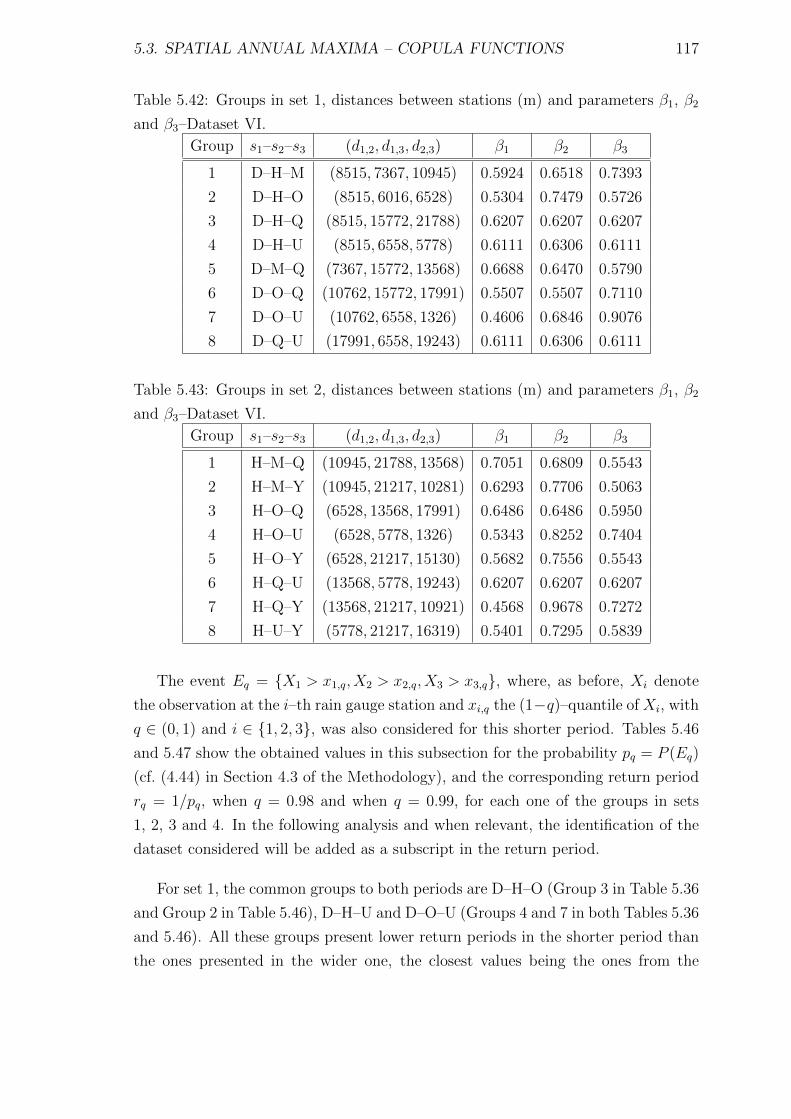
5.3. SPATIAL ANNUAL MAXIMA – COPULA FUNCTIONS 117
Table 5.42: Groups in set 1, distances between stations (m) and parameters β1, β2
and β3–Dataset VI.
Group s1–s2–s3 (d1,2, d1,3, d2,3) β1 β2 β3
1 D–H–M (8515, 7367, 10945) 0.5924 0.6518 0.7393
2 D–H–O (8515, 6016, 6528) 0.5304 0.7479 0.5726
3 D–H–Q (8515, 15772, 21788) 0.6207 0.6207 0.6207
4 D–H–U (8515, 6558, 5778) 0.6111 0.6306 0.6111
5 D–M–Q (7367, 15772, 13568) 0.6688 0.6470 0.5790
6 D–O–Q (10762, 15772, 17991) 0.5507 0.5507 0.7110
7 D–O–U (10762, 6558, 1326) 0.4606 0.6846 0.9076
8 D–Q–U (17991, 6558, 19243) 0.6111 0.6306 0.6111
Table 5.43: Groups in set 2, distances between stations (m) and parameters β1, β2
and β3–Dataset VI.
Group s1–s2–s3 (d1,2, d1,3, d2,3) β1 β2 β3
1 H–M–Q (10945, 21788, 13568) 0.7051 0.6809 0.5543
2 H–M–Y (10945, 21217, 10281) 0.6293 0.7706 0.5063
3 H–O–Q (6528, 13568, 17991) 0.6486 0.6486 0.5950
4 H–O–U (6528, 5778, 1326) 0.5343 0.8252 0.7404
5 H–O–Y (6528, 21217, 15130) 0.5682 0.7556 0.5543
6 H–Q–U (13568, 5778, 19243) 0.6207 0.6207 0.6207
7 H–Q–Y (13568, 21217, 10921) 0.4568 0.9678 0.7272
8 H–U–Y (5778, 21217, 16319) 0.5401 0.7295 0.5839
The event Eq = {X1 > x1,q, X2 > x2,q, X3 > x3,q}, where, as before, Xi denote
the observation at the i–th rain gauge station and xi,q the (1−q)–quantile of Xi, with
q ∈ (0, 1) and i ∈ {1, 2, 3}, was also considered for this shorter period. Tables 5.46
and 5.47 show the obtained values in this subsection for the probability pq = P (Eq)
(cf. (4.44) in Section 4.3 of the Methodology), and the corresponding return period
rq = 1/pq, when q = 0.98 and when q = 0.99, for each one of the groups in sets
1, 2, 3 and 4. In the following analysis and when relevant, the identification of the
dataset considered will be added as a subscript in the return period.
For set 1, the common groups to both periods are D–H–O (Group 3 in Table 5.36
and Group 2 in Table 5.46), D–H–U and D–O–U (Groups 4 and 7 in both Tables 5.36
and 5.46). All these groups present lower return periods in the shorter period than
the ones presented in the wider one, the closest values being the ones from the
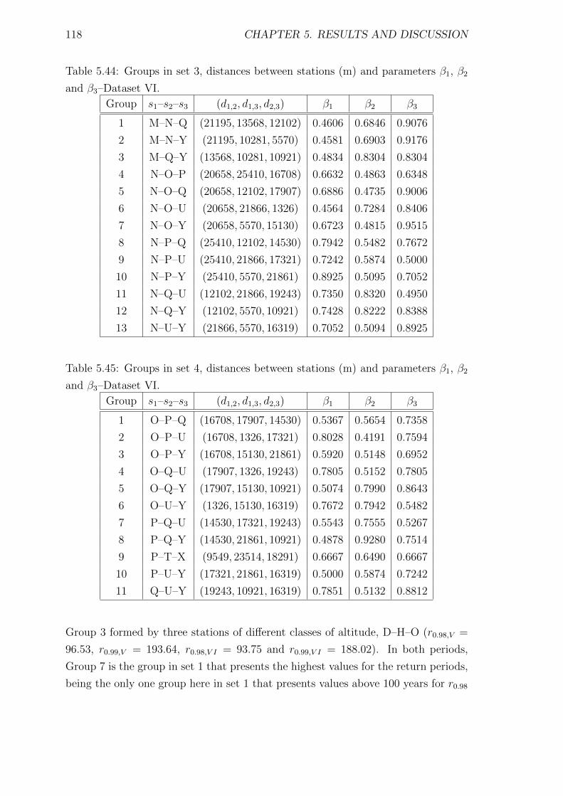
118 CHAPTER 5. RESULTS AND DISCUSSION
Table 5.44: Groups in set 3, distances between stations (m) and parameters β1, β2
and β3–Dataset VI.
Group s1–s2–s3 (d1,2, d1,3, d2,3) β1 β2 β3
1 M–N–Q (21195, 13568, 12102) 0.4606 0.6846 0.9076
2 M–N–Y (21195, 10281, 5570) 0.4581 0.6903 0.9176
3 M–Q–Y (13568, 10281, 10921) 0.4834 0.8304 0.8304
4 N–O–P (20658, 25410, 16708) 0.6632 0.4863 0.6348
5 N–O–Q (20658, 12102, 17907) 0.6886 0.4735 0.9006
6 N–O–U (20658, 21866, 1326) 0.4564 0.7284 0.8406
7 N–O–Y (20658, 5570, 15130) 0.6723 0.4815 0.9515
8 N–P–Q (25410, 12102, 14530) 0.7942 0.5482 0.7672
9 N–P–U (25410, 21866, 17321) 0.7242 0.5874 0.5000
10 N–P–Y (25410, 5570, 21861) 0.8925 0.5095 0.7052
11 N–Q–U (12102, 21866, 19243) 0.7350 0.8320 0.4950
12 N–Q–Y (12102, 5570, 10921) 0.7428 0.8222 0.8388
13 N–U–Y (21866, 5570, 16319) 0.7052 0.5094 0.8925
Table 5.45: Groups in set 4, distances between stations (m) and parameters β1, β2
and β3–Dataset VI.
Group s1–s2–s3 (d1,2, d1,3, d2,3) β1 β2 β3
1 O–P–Q (16708, 17907, 14530) 0.5367 0.5654 0.7358
2 O–P–U (16708, 1326, 17321) 0.8028 0.4191 0.7594
3 O–P–Y (16708, 15130, 21861) 0.5920 0.5148 0.6952
4 O–Q–U (17907, 1326, 19243) 0.7805 0.5152 0.7805
5 O–Q–Y (17907, 15130, 10921) 0.5074 0.7990 0.8643
6 O–U–Y (1326, 15130, 16319) 0.7672 0.7942 0.5482
7 P–Q–U (14530, 17321, 19243) 0.5543 0.7555 0.5267
8 P–Q–Y (14530, 21861, 10921) 0.4878 0.9280 0.7514
9 P–T–X (9549, 23514, 18291) 0.6667 0.6490 0.6667
10 P–U–Y (17321, 21861, 16319) 0.5000 0.5874 0.7242
11 Q–U–Y (19243, 10921, 16319) 0.7851 0.5132 0.8812
Group 3 formed by three stations of different classes of altitude, D–H–O (r0.98,V =
96.53, r0.99,V = 193.64, r0.98,V I = 93.75 and r0.99,V I = 188.02). In both periods,
Group 7 is the group in set 1 that presents the highest values for the return periods,
being the only one group here in set 1 that presents values above 100 years for r0.98
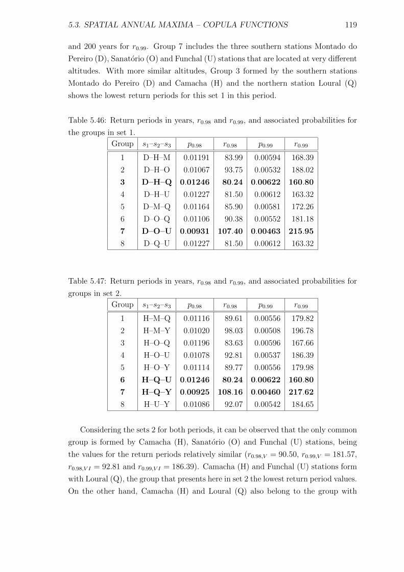
5.3. SPATIAL ANNUAL MAXIMA – COPULA FUNCTIONS 119
and 200 years for r0.99. Group 7 includes the three southern stations Montado do
Pereiro (D), Sanatorio (O) and Funchal (U) stations that are located at very different
altitudes. With more similar altitudes, Group 3 formed by the southern stations
Montado do Pereiro (D) and Camacha (H) and the northern station Loural (Q)
shows the lowest return periods for this set 1 in this period.
Table 5.46: Return periods in years, r0.98 and r0.99, and associated probabilities for
the groups in set 1.
Group s1–s2–s3 p0.98 r0.98 p0.99 r0.99
1 D–H–M 0.01191 83.99 0.00594 168.39
2 D–H–O 0.01067 93.75 0.00532 188.02
3 D–H–Q 0.01246 80.24 0.00622 160.80
4 D–H–U 0.01227 81.50 0.00612 163.32
5 D–M–Q 0.01164 85.90 0.00581 172.26
6 D–O–Q 0.01106 90.38 0.00552 181.18
7 D–O–U 0.00931 107.40 0.00463 215.95
8 D–Q–U 0.01227 81.50 0.00612 163.32
Table 5.47: Return periods in years, r0.98 and r0.99, and associated probabilities for
groups in set 2.
Group s1–s2–s3 p0.98 r0.98 p0.99 r0.99
1 H–M–Q 0.01116 89.61 0.00556 179.82
2 H–M–Y 0.01020 98.03 0.00508 196.78
3 H–O–Q 0.01196 83.63 0.00596 167.66
4 H–O–U 0.01078 92.81 0.00537 186.39
5 H–O–Y 0.01114 89.77 0.00556 179.98
6 H–Q–U 0.01246 80.24 0.00622 160.80
7 H–Q–Y 0.00925 108.16 0.00460 217.62
8 H–U–Y 0.01086 92.07 0.00542 184.65
Considering the sets 2 for both periods, it can be observed that the only common
group is formed by Camacha (H), Sanatorio (O) and Funchal (U) stations, being
the values for the return periods relatively similar (r0.98,V = 90.50, r0.99,V = 181.57,
r0.98,V I = 92.81 and r0.99,V I = 186.39). Camacha (H) and Funchal (U) stations form
with Loural (Q), the group that presents here in set 2 the lowest return period values.
On the other hand, Camacha (H) and Loural (Q) also belong to the group with
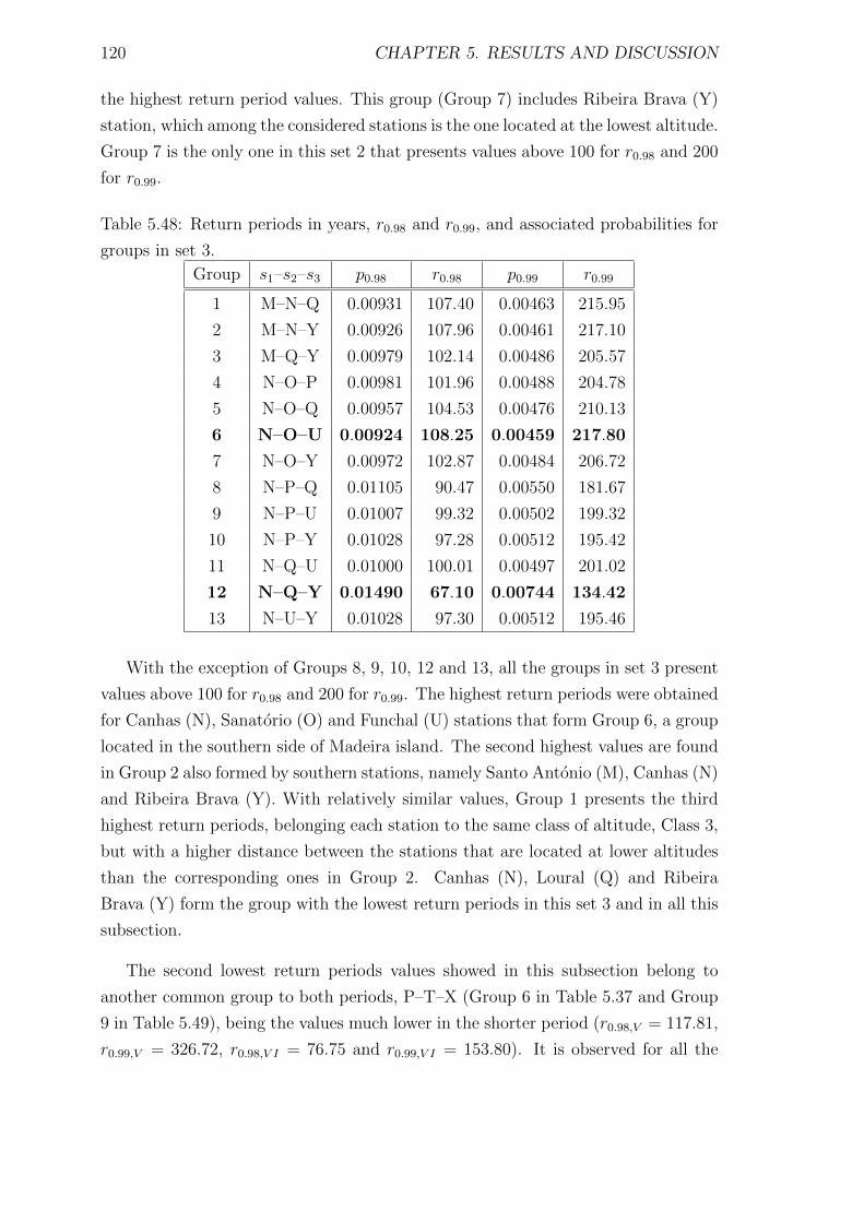
120 CHAPTER 5. RESULTS AND DISCUSSION
the highest return period values. This group (Group 7) includes Ribeira Brava (Y)
station, which among the considered stations is the one located at the lowest altitude.
Group 7 is the only one in this set 2 that presents values above 100 for r0.98 and 200
for r0.99.
Table 5.48: Return periods in years, r0.98 and r0.99, and associated probabilities for
groups in set 3.
Group s1–s2–s3 p0.98 r0.98 p0.99 r0.99
1 M–N–Q 0.00931 107.40 0.00463 215.95
2 M–N–Y 0.00926 107.96 0.00461 217.10
3 M–Q–Y 0.00979 102.14 0.00486 205.57
4 N–O–P 0.00981 101.96 0.00488 204.78
5 N–O–Q 0.00957 104.53 0.00476 210.13
6 N–O–U 0.00924 108.25 0.00459 217.80
7 N–O–Y 0.00972 102.87 0.00484 206.72
8 N–P–Q 0.01105 90.47 0.00550 181.67
9 N–P–U 0.01007 99.32 0.00502 199.32
10 N–P–Y 0.01028 97.28 0.00512 195.42
11 N–Q–U 0.01000 100.01 0.00497 201.02
12 N–Q–Y 0.01490 67.10 0.00744 134.42
13 N–U–Y 0.01028 97.30 0.00512 195.46
With the exception of Groups 8, 9, 10, 12 and 13, all the groups in set 3 present
values above 100 for r0.98 and 200 for r0.99. The highest return periods were obtained
for Canhas (N), Sanatorio (O) and Funchal (U) stations that form Group 6, a group
located in the southern side of Madeira island. The second highest values are found
in Group 2 also formed by southern stations, namely Santo Antonio (M), Canhas (N)
and Ribeira Brava (Y). With relatively similar values, Group 1 presents the third
highest return periods, belonging each station to the same class of altitude, Class 3,
but with a higher distance between the stations that are located at lower altitudes
than the corresponding ones in Group 2. Canhas (N), Loural (Q) and Ribeira
Brava (Y) form the group with the lowest return periods in this set 3 and in all this
subsection.
The second lowest return periods values showed in this subsection belong to
another common group to both periods, P–T–X (Group 6 in Table 5.37 and Group
9 in Table 5.49), being the values much lower in the shorter period (r0.98,V = 117.81,
r0.99,V = 326.72, r0.98,V I = 76.75 and r0.99,V I = 153.80). It is observed for all the
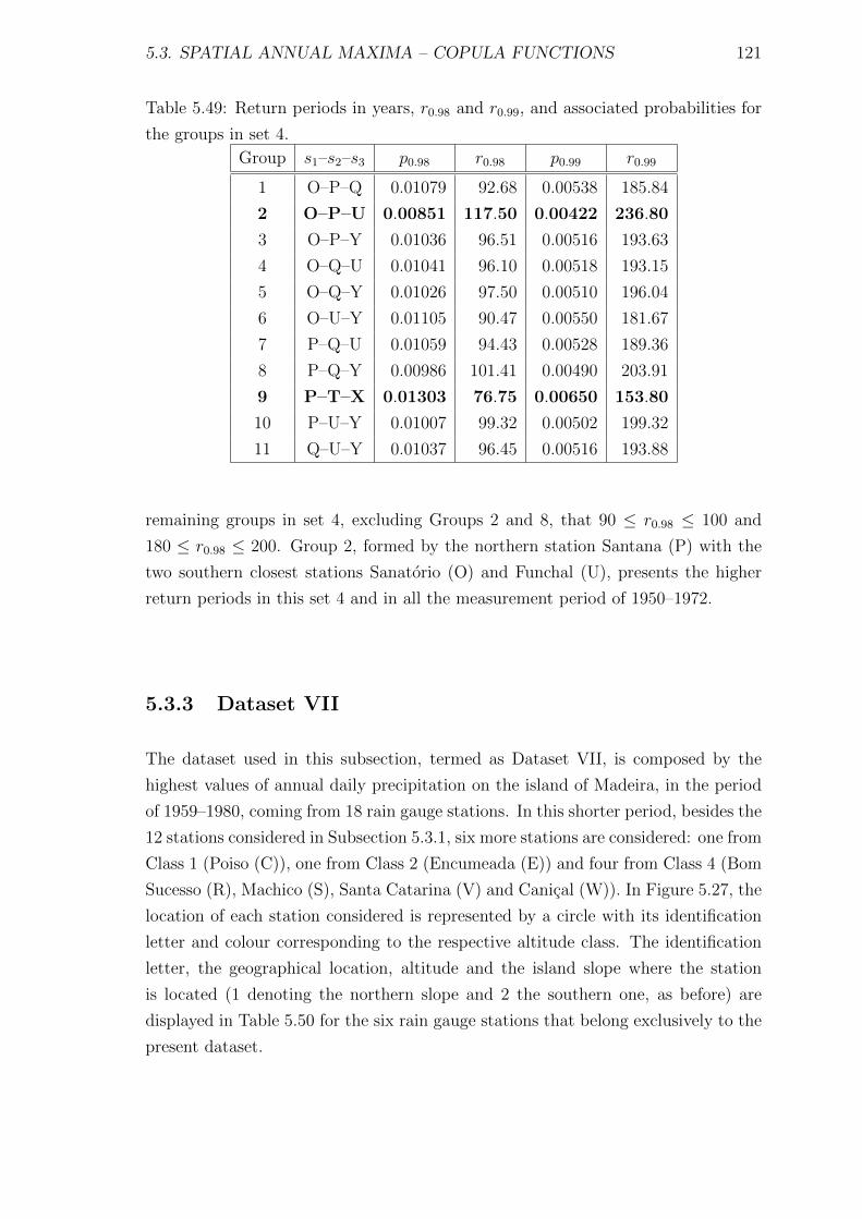
5.3. SPATIAL ANNUAL MAXIMA – COPULA FUNCTIONS 121
Table 5.49: Return periods in years, r0.98 and r0.99, and associated probabilities for
the groups in set 4.
Group s1–s2–s3 p0.98 r0.98 p0.99 r0.99
1 O–P–Q 0.01079 92.68 0.00538 185.84
2 O–P–U 0.00851 117.50 0.00422 236.80
3 O–P–Y 0.01036 96.51 0.00516 193.63
4 O–Q–U 0.01041 96.10 0.00518 193.15
5 O–Q–Y 0.01026 97.50 0.00510 196.04
6 O–U–Y 0.01105 90.47 0.00550 181.67
7 P–Q–U 0.01059 94.43 0.00528 189.36
8 P–Q–Y 0.00986 101.41 0.00490 203.91
9 P–T–X 0.01303 76.75 0.00650 153.80
10 P–U–Y 0.01007 99.32 0.00502 199.32
11 Q–U–Y 0.01037 96.45 0.00516 193.88
remaining groups in set 4, excluding Groups 2 and 8, that 90 ≤ r0.98 ≤ 100 and
180 ≤ r0.98 ≤ 200. Group 2, formed by the northern station Santana (P) with the
two southern closest stations Sanatorio (O) and Funchal (U), presents the higher
return periods in this set 4 and in all the measurement period of 1950–1972.
5.3.3 Dataset VII
The dataset used in this subsection, termed as Dataset VII, is composed by the
highest values of annual daily precipitation on the island of Madeira, in the period
of 1959–1980, coming from 18 rain gauge stations. In this shorter period, besides the
12 stations considered in Subsection 5.3.1, six more stations are considered: one from
Class 1 (Poiso (C)), one from Class 2 (Encumeada (E)) and four from Class 4 (Bom
Sucesso (R), Machico (S), Santa Catarina (V) and Canical (W)). In Figure 5.27, the
location of each station considered is represented by a circle with its identification
letter and colour corresponding to the respective altitude class. The identification
letter, the geographical location, altitude and the island slope where the station
is located (1 denoting the northern slope and 2 the southern one, as before) are
displayed in Table 5.50 for the six rain gauge stations that belong exclusively to the
present dataset.
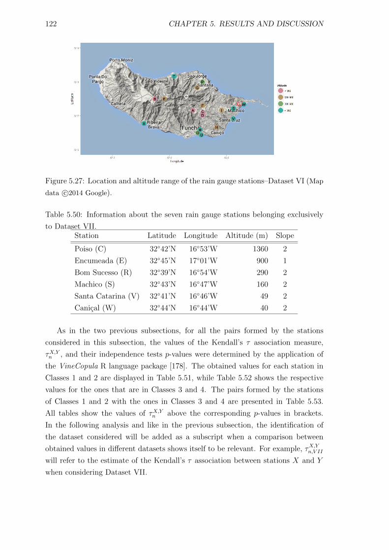
122 CHAPTER 5. RESULTS AND DISCUSSION
Figure 5.27: Location and altitude range of the rain gauge stations–Dataset VI (Map
data c©2014 Google).
Table 5.50: Information about the seven rain gauge stations belonging exclusively
to Dataset VII.Station Latitude Longitude Altitude (m) Slope
Poiso (C) 32◦42’N 16◦53’W 1360 2
Encumeada (E) 32◦45’N 17◦01’W 900 1
Bom Sucesso (R) 32◦39’N 16◦54’W 290 2
Machico (S) 32◦43’N 16◦47’W 160 2
Santa Catarina (V) 32◦41’N 16◦46’W 49 2
Canical (W) 32◦44’N 16◦44’W 40 2
As in the two previous subsections, for all the pairs formed by the stations
considered in this subsection, the values of the Kendall’s τ association measure,
τX,Yn , and their independence tests p-values were determined by the application of
the VineCopula R language package [178]. The obtained values for each station in
Classes 1 and 2 are displayed in Table 5.51, while Table 5.52 shows the respective
values for the ones that are in Classes 3 and 4. The pairs formed by the stations
of Classes 1 and 2 with the ones in Classes 3 and 4 are presented in Table 5.53.
All tables show the values of τX,Yn above the corresponding p-values in brackets.
In the following analysis and like in the previous subsection, the identification of
the dataset considered will be added as a subscript when a comparison between
obtained values in different datasets shows itself to be relevant. For example, τX,Yn,V II
will refer to the estimate of the Kendall’s τ association between stations X and Y
when considering Dataset VII.
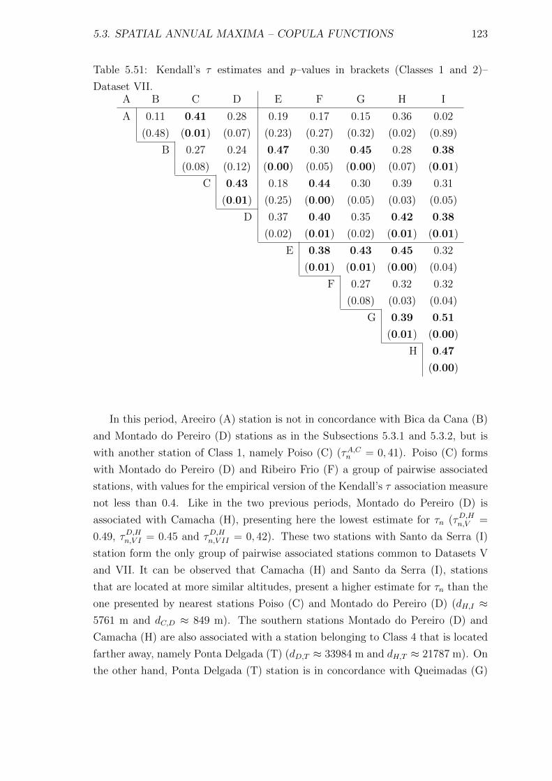
5.3. SPATIAL ANNUAL MAXIMA – COPULA FUNCTIONS 123
Table 5.51: Kendall’s τ estimates and p–values in brackets (Classes 1 and 2)–
Dataset VII.A B C D E F G H I
A 0.11 0.41 0.28 0.19 0.17 0.15 0.36 0.02
(0.48) (0.01) (0.07) (0.23) (0.27) (0.32) (0.02) (0.89)
B 0.27 0.24 0.47 0.30 0.45 0.28 0.38
(0.08) (0.12) (0.00) (0.05) (0.00) (0.07) (0.01)
C 0.43 0.18 0.44 0.30 0.39 0.31
(0.01) (0.25) (0.00) (0.05) (0.03) (0.05)
D 0.37 0.40 0.35 0.42 0.38
(0.02) (0.01) (0.02) (0.01) (0.01)
E 0.38 0.43 0.45 0.32
(0.01) (0.01) (0.00) (0.04)
F 0.27 0.32 0.32
(0.08) (0.03) (0.04)
G 0.39 0.51
(0.01) (0.00)
H 0.47
(0.00)
In this period, Areeiro (A) station is not in concordance with Bica da Cana (B)
and Montado do Pereiro (D) stations as in the Subsections 5.3.1 and 5.3.2, but is
with another station of Class 1, namely Poiso (C) (τA,Cn = 0, 41). Poiso (C) forms
with Montado do Pereiro (D) and Ribeiro Frio (F) a group of pairwise associated
stations, with values for the empirical version of the Kendall’s τ association measure
not less than 0.4. Like in the two previous periods, Montado do Pereiro (D) is
associated with Camacha (H), presenting here the lowest estimate for τn (τD,Hn,V =
0.49, τD,Hn,V I = 0.45 and τD,Hn,V II = 0, 42). These two stations with Santo da Serra (I)
station form the only group of pairwise associated stations common to Datasets V
and VII. It can be observed that Camacha (H) and Santo da Serra (I), stations
that are located at more similar altitudes, present a higher estimate for τn than the
one presented by nearest stations Poiso (C) and Montado do Pereiro (D) (dH,I ≈5761 m and dC,D ≈ 849 m). The southern stations Montado do Pereiro (D) and
Camacha (H) are also associated with a station belonging to Class 4 that is located
farther away, namely Ponta Delgada (T) (dD,T ≈ 33984 m and dH,T ≈ 21787 m). On
the other hand, Ponta Delgada (T) station is in concordance with Queimadas (G)
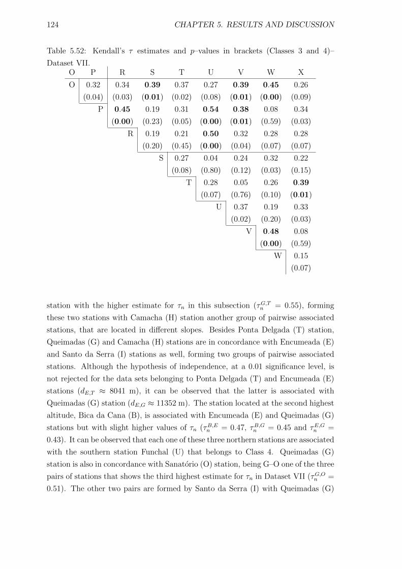
124 CHAPTER 5. RESULTS AND DISCUSSION
Table 5.52: Kendall’s τ estimates and p–values in brackets (Classes 3 and 4)–
Dataset VII.O P R S T U V W X
O 0.32 0.34 0.39 0.37 0.27 0.39 0.45 0.26
(0.04) (0.03) (0.01) (0.02) (0.08) (0.01) (0.00) (0.09)
P 0.45 0.19 0.31 0.54 0.38 0.08 0.34
(0.00) (0.23) (0.05) (0.00) (0.01) (0.59) (0.03)
R 0.19 0.21 0.50 0.32 0.28 0.28
(0.20) (0.45) (0.00) (0.04) (0.07) (0.07)
S 0.27 0.04 0.24 0.32 0.22
(0.08) (0.80) (0.12) (0.03) (0.15)
T 0.28 0.05 0.26 0.39
(0.07) (0.76) (0.10) (0.01)
U 0.37 0.19 0.33
(0.02) (0.20) (0.03)
V 0.48 0.08
(0.00) (0.59)
W 0.15
(0.07)
station with the higher estimate for τn in this subsection (τG,Tn = 0.55), forming
these two stations with Camacha (H) station another group of pairwise associated
stations, that are located in different slopes. Besides Ponta Delgada (T) station,
Queimadas (G) and Camacha (H) stations are in concordance with Encumeada (E)
and Santo da Serra (I) stations as well, forming two groups of pairwise associated
stations. Although the hypothesis of independence, at a 0.01 significance level, is
not rejected for the data sets belonging to Ponta Delgada (T) and Encumeada (E)
stations (dE,T ≈ 8041 m), it can be observed that the latter is associated with
Queimadas (G) station (dE,G ≈ 11352 m). The station located at the second highest
altitude, Bica da Cana (B), is associated with Encumeada (E) and Queimadas (G)
stations but with slight higher values of τn (τB,En = 0.47, τB,Gn = 0.45 and τE,Gn =
0.43). It can be observed that each one of these three northern stations are associated
with the southern station Funchal (U) that belongs to Class 4. Queimadas (G)
station is also in concordance with Sanatorio (O) station, being G–O one of the three
pairs of stations that shows the third highest estimate for τn in Dataset VII (τG,On =
0.51). The other two pairs are formed by Santo da Serra (I) with Queimadas (G)
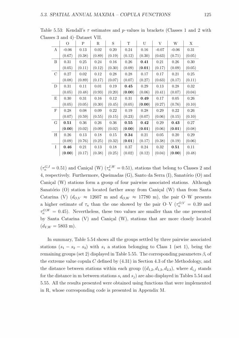
5.3. SPATIAL ANNUAL MAXIMA – COPULA FUNCTIONS 125
Table 5.53: Kendall’s τ estimates and p–values in brackets (Classes 1 and 2 with
Classes 3 and 4)–Dataset VII.O P R S T U V W X
A -0.06 0.13 0.02 0.20 0.24 0.16 -0.07 -0.06 0.31
(0.67) (0.38) (0.89) (0.19) (0.12) (0.30) (0.63) (0.71) (0.05)
B 0.31 0.25 0.24 0.16 0.26 0.41 0.21 0.26 0.30
(0.05) (0.11) (0.12) (0.30) (0.09) (0.01) (0.17) (0.09) (0.05)
C 0.27 0.02 0.12 0.28 0.28 0.17 0.17 0.21 0.25
(0.08) (0.89) (0.17) (0.07) (0.07) (0.27) (0.63) (0.17) (0.11)
D 0.31 0.11 0.01 0.19 0.45 0.29 0.13 0.28 0.32
(0.05) (0.48) (0.93) (0.20) (0.00) (0.06) (0.41) (0.07) (0.04)
E 0.30 0.31 0.16 0.12 0.31 0.49 0.17 0.05 0.26
(0.05) (0.05) (0.30) (0.45) (0.05) (0.00) (0.27) (0.76) (0.10)
F 0.28 0.08 0.09 0.22 0.19 0.28 0.29 0.22 0.26
(0.07) (0.59) (0.55) (0.15) (0.23) (0.07) (0.06) (0.15) (0.10)
G 0.51 0.36 0.26 0.36 0.55 0.42 0.29 0.43 0.27
(0.00) (0.02) (0.09) (0.02) (0.00) (0.01) (0.06) (0.01) (0.08)
H 0.26 0.13 0.18 0.15 0.34 0.21 0.05 0.20 0.29
(0.09) (0.76) (0.25) (0.32) (0.01) (0.17) (0.38) (0.19) (0.06)
I 0.46 0.21 0.13 0.18 0.37 0.24 0.32 0.51 0.11
(0.00) (0.17) (0.38) (0.25) (0.02) (0.12) (0.04) (0.00) (0.48)
(τG,In = 0.51) and Canical (W) (τ I,Wn = 0.51), stations that belong to Classes 2 and
4, respectively. Furthermore, Queimadas (G), Santo da Serra (I), Sanatorio (O) and
Canical (W) stations form a group of four pairwise associated stations. Although
Sanatorio (O) station is located farther away from Canical (W) than from Santa
Catarina (V) (dO,V ≈ 12607 m and dO,W ≈ 17780 m), the pair O–W presents
a higher estimate of τn than the one showed by the pair O–V (τO,Vn = 0.39 and
τO,Wn = 0.45). Nevertheless, these two values are smaller than the one presented
by Santa Catarina (V) and Canical (W), stations that are more closely located
(dV,W = 5803 m).
In summary, Table 5.54 shows all the groups settled by three pairwise associated
stations (s1 − s2 − s3) with s1 a station belonging to Class 1 (set 1), being the
remaining groups (set 2) displayed in Table 5.55. The corresponding parameters βi of
the extreme value copula C defined by (4.31) in Section 4.3 of the Methodology, and
the distance between stations within each group ((d1,2, d1,3, d2,3), where di,j stands
for the distance in m between stations si and sj) are also displayed in Tables 5.54 and
5.55. All the results presented were obtained using functions that were implemented
in R, whose corresponding code is presented in Appendix M.

126 CHAPTER 5. RESULTS AND DISCUSSION
Table 5.54: Groups in set 1, distance between stations (m) and parameters β1, β2
and β3–Dataset VII.
Group s1-s2-s3 (d1,2, d1,3, d2,3) β1 β2 β3
1 B–E–G (3170, 14348, 11352) 0.6613 0.6190 0.5848
2 B–E–U (3170, 19250, 16893) 0.5672 0.7327 0.5966
3 B–G–I (14348, 22200, 10889) 0.5137 0.7839 0.5934
4 B–G–U (14348, 19250, 15517) 0.6097 0.6321 0.5559
5 C–D–F (849, 2426, 3242) 0.5802 0.6455 0.5629
6 D–H–I (8515, 6538, 5761) 0.5148 0.6952 0.5920
7 D–H–T (8515, 19379, 21787) 0.7513 0.4878 0.5288
Table 5.55: Groups in set 2, distance between stations (m) and parameters β1, β2
and β3–Dataset VII.
Group s1-s2-s3 (d1,2, d1,3, d2,3) β1 β2 β3
1 E–G–H (11352, 19554, 14440) 0.6703 0.5453 0.5779
2 E–G–U (11352, 16893, 15517) 0.6699 0.5456 0.6460
3 G–H–I (14440, 10889, 5761) 0.5887 0.5361 0.7923
4 G–H–T (14440, 8494, 21787) 0.8193 0.4267 0.6259
5 G–I–O (10889, 14774, 10762) 0.7279 0.6301 0.6301
6 G–I–W (10889, 16301, 7600) 0.6014 0.7704 0.6014
7 G–O–W (14774, 16301, 17780) 0.6527 0.6999 0.5576
8 I–O–W (10762, 7600, 17780) 0.6867 0.5822 0.6647
9 O–V–W (12607, 17780, 5803) 0.5401 0.5839 0.7295
The event Eq = {X1 > x1,q, X2 > x2,q, X3 > x3,q}, where Xi denote the
observation at the i–th rain gauge station and xi,q the (1− q)–quantile of Xi, with
q ∈ (0, 1) and i ∈ {1, 2, 3}, was also considered for this subsection. For q = 0.98
and q = 0.99, Tables 5.56 and 5.57 show the obtained values in this subsection of
the probability pq = P (Eq) (cf. (4.44) in Section 4.3 of the Methodology), and the
corresponding return period rq = 1/pq for each one of the groups in sets 1 and 2,
respectively.
In set 1, the lowest return period values obtained correspond to Group 1 (r0.98 =
85.10 and r0.99 = 170.60), a group formed by the three northern stations Bica da
Cana (B), Encumeada (E) and Queimadas (G). The first two stations also belong
to the group that presents the second lowest return period (r0.98 = 87.73 and r0.99 =
175.88), being the third station, Funchal (U), located in the southern side of the
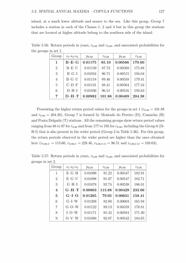
5.3. SPATIAL ANNUAL MAXIMA – COPULA FUNCTIONS 127
island, at a much lower altitude and nearer to the sea. Like this group, Group 7
includes a station in each of the Classes 1, 2 and 4 but in this group the stations
that are located at higher altitude belong to the southern side of the island.
Table 5.56: Return periods in years, r0.98 and r0.99, and associated probabilities for
the groups in set 1.
Group s1-s2-s3 p0.98 r0.98 p0.99 r0.99
1 B–E–G 0.01175 85.10 0.00586 170.60
2 B–E–U 0.01139 87.73 0.00569 175.88
3 B–G–I 0.01034 96.71 0.00515 194.04
4 B–G–U 0.01118 89.46 0.00558 179.41
5 C–D–F 0.01131 88.41 0.00564 177.24
6 D–H–I 0.01036 96.51 0.00516 193.63
7 D–H–T 0.00982 101.88 0.00489 204.38
Presenting the higher return period values for the groups in set 1 (r0.98 = 101.88
and r0.99 = 204.38), Group 7 is formed by Montado do Pereiro (D), Camacha (H)
and Ponta Delgada (T) stations. All the remaining groups show return period values
ranging from 88 to 97 for r0.98 and from 177 to 195 for r0.98, including the Group 6 (D-
H-I) that is also present in the wider period (Group 2 in Table 5.36). For this group,
the return periods observed in the wider period are higher than the ones obtained
here (r0.98,V = 113.60, r0.99,V = 228.46, r0.98,V II = 96.51 and r0.99,V II = 193.63).
Table 5.57: Return periods in years, r0.98 and r0.99, and associated probabilities for
groups in set 2.
Group s1-s2-s3 p0.98 r0.98 p0.99 r0.99
1 E–G–H 0.01096 91.22 0.00547 182.91
2 E–G–U 0.01098 91.07 0.00547 182.71
3 G–H–I 0.01078 92.74 0.00538 186.01
4 G–H–T 0.00863 115.88 0.00429 233.06
5 G–I–O 0.01265 79.05 0.00631 158.41
6 G–I–W 0.01208 82.80 0.00603 165.94
7 G–O–W 0.01122 89.13 0.00559 178.81
8 I–O–W 0.01171 85.42 0.00584 171.30
9 O–V–W 0.01086 92.07 0.00542 184.65
128 CHAPTER 5. RESULTS AND DISCUSSION
In set 2, the highest and the lowest return period values obtained correspond
to the Groups 4 and 5, respectively, being Queimadas (G) a common station to
the two groups. Besides Queimadas (G) station, Group 4 includes Camacha (H), a
southern station that belongs to the same class of altitude, and Ponta Delgada (T)
a station that is located in the northern side of the island and nearest the sea. The
southern station Santo da Serra (I) belongs to Class 2 like Queimadas (G), but the
third station of Group 5, Sanatorio (O), is included in Class 4 and is located in the
southern side. The return periods for Group 4 (r0.98 = 115.88 and r0.99 = 233.06)
show the highest values observed in set 2 and in all the period 1959–1980. The
lowest values for the same period are shown by Group 5 of set 2: r0.98 = 79.05 and
r0.99 = 158.41. All the remaining groups present return period values ranging from
82 to 93 for r0.98 and from 165 to 187 for r0.99.
Chapter 6
Conclusion
Early work in hydrology usually assumed a Gumbel distribution for the block
maxima or equivalently an exponential distribution for the excesses over a high
threshold [124]. However, since the earlier years of the extreme value theory
there was the notion that the Gumbel distribution tends to underestimate the
magnitude of extreme rainfall events and the use of the GEV distribution has been
recommended for rainfall frequency since 1995 [224]. On the other hand, the GPD
has been suggested for the excess distribution function since a long time ago, being
the definition of the GPD traceable back to the work of Pickands [171] in 1975.
Statistics of extremes for independent and identical random variables were applied
following a parametric approach, but a semi–parametric one has gained its space in
the most recent times. Under the PORT semi-parametric approach, and also under
the classical Gumbel’s and POT approaches, an analysis of rainfall values collected
in Madeira Island over different periods of time was done in this thesis. Also, a
study about the dependence of annual maximum rainfall in Madeira Island by
means of the Kendall’s τ association measure was carried out, and the multivariate
extremes were addressed through an EVC approach.
Using Gumbel’s approach, GEV parameters estimates for annual maxima of daily
rainfall in Madeira Island are provided by ML and PWM methods. For the annual
maxima data drawn from the seven rain gauge stations maintained in the island
by IPMA, the hyphotesis of Gumbel distribution was tested by the likelihood ratio
test and a test presented by Hosking et al. [119], both methods leading to the same
conclusions. For the distributions corresponding to Areeiro (A), Santo da Serra (I),
Santana (P), Funchal (U) and Santa Catarina (V), there is not significant evidence
to choose the GEV model, with γ 6= 0, instead of the Gumbel model. Nevertheless,
it can be observed that the ML estimate for the shape parameter γ for each of
129
130 CHAPTER 6. CONCLUSION
these stations is not equal to zero and that the GEV location and scale parameters
estimates are similar for both methods, but that is not the case when the Gumbel
distribution is chosen. Therefore, in these particular cases, the option taken was to
determine the estimates for the 50– and 100–year return levels using the ML method
and considering the GEV distribution.
The estimates for the shape parameter range from −0.3 to 0.3, being greater
than 0.09 for the two stations located at the lowest altitudes and nearest the sea,
namely, Santa Catarina (V) and Lugar de Baixo (X) stations. The estimate for
γ is also positive for the Santana (P) station but it is closer to zero. Data from
Areeiro (A), Bica da Cana (B), Santo da Serra (I) and Funchal (U) rain gauge
stations revealed negative estimates for the shape parameter, being the lowest values
presented by Bica da Cana (B) station. Exploring the possibility of the existence of
trends, a significant evidence for a linear trend in the location parameter was only
found for the Areeiro (A) station data. Without considering this trend, this rain
gauge station is the one that shows the higher estimates for the location parameter,
with values approximately equal to 159 mm, for both methods considered. Bica
da Cana (B) presents lower values for the location parameter estimates than the
ones from Areeiro (A), but that is not the case for the values of the scale parameter
estimates. However, it is Santo da Serra (I) station the one that presents the highest
scale parameter estimates, having values approximately equal to 116 mm for the
location parameter estimates. Although, Santana (P) presents values for location
parameter estimates that are nearly half of the ones presented by Areeiro (A), the
values for the scale parameter estimates are still slightly higher than the ones from
this station. The stations below 300 m present lower location and scale estimates
with values below 55 mm and 25 mm, respectively. The lower values correspond to
the rain gauge station located at the lowest altitude, namely Lugar de Baixo (X). It
turns out this is the station that presents the second lowest estimate values for the
50– and 100–year return level, being the lowest ones showed by Funchal (U) station.
On the other hand, the highest estimates for the 50– and 100–year return levels are
showed by Areeiro (A) station. Although Santo da Serra (I) station is located in a
lower altitude than Bica da Cana (B), it presents higher estimates for the 50– and
100–year return levels than this station.
Also in this thesis, tests based on the likelihood ratio statistic and the PWM
were used to test the hypothesis of a Gumbel distribution for the annual 1-day
maximum rainfall data, from 25 rain gauge stations, maintained in the past by
the General Council of the Autonomous District of Funchal. From the rainfall

131
records drawn from these rain gauge stations located in the northern and southern
hillsides of the island, annual maxima datasets with 22 to 31 years of extension were
obtained. Although most of the rain gauge stations considered are deactivated, and
consequently the rainfall time series are relatively short, it is important to analyse
all the available data, given the number of major flash flood events reported so far
in Madeira Island. The most significant one among the most recent events of this
nature occurred on the 20th of February 2010, with 146.9 mm observed in Funchal
and 333.8 mm in Areeiro [70]. Given the GEV estimates obtained in this work
by ML, these values correspond to return periods of approximately 79 years and
292 years, respectively, or 70 years and 297 years when GEV estimates by PWM are
used. Although for almost all rainfall data series there was no significant evidence to
choose the GEV distribution, non Gumbel, in opposition to the Gumbel distribution,
GEV parameters estimates by ML and PWM methods were provided in this work
given that the corresponding shape parameters estimates are not equal to zero and
that location and scale GEV estimates are relatively similar for both methods. The
hypothesis of a Gumbel distribution was tested by the likelihood ratio test and by
the test presented by Hosking et al. [119], and the same conclusions were obtained
for both methods, with the exception of the data from Queimadas (G) and Santo
Antonio (M) rain gauge stations. For the latter two stations and also for Bica da
Cana (B), Curral das Freiras (K), Canhas (N), Machico (S), Canical (W) and Ribeira
Brava (Y) stations, there was evidence of a linear trend in one or two parameters
when modelling the corresponding annual maxima by the GEV distribution. For
Bica da Cana (B) and Ribeira Brava (Y) stations, a significant evidence for a linear
trend in location and scale parameters was found in the data independently of the
model chosen. Estimates for the 50– and 100–year return levels were also determined
for all rain gauge stations data using the GEV parameter estimates obtained from
both methods.
The parameters and return level estimates, regardless of the method used to
obtain them, suggest a complex characterization of the spatial distribution of
extreme rainfall in Madeira Island. It seems that there is a simultaneous influence
of factors such as altitude, proximity to the sea, distance, and location in nearby
hillsides or in the northern or the southern part of the island. Besides, there are
differences in the return levels estimates according to the method applied, except
for Areeiro (A), Ribeiro Frio (F), Porto Moniz (J), Ponta do Pargo (L), Santo
Antonio (M) and Ribeira Brava (Y) rain gauge stations for which the estimates
are approximately similar. Nevertheless, it can be observed that the 50– and
132 CHAPTER 6. CONCLUSION
100–year return levels estimates are greater than 242 and 255 mm, respectively,
for the seven rain gauge stations located farther from the sea Areeiro (A), Bica da
Cana (B), Poiso (C), Montado do Pereiro (D), Encumeada (E), Ribeiro Frio (F)
and Loural (Q). The same can be observed for three more stations, Porto Moniz (J),
Santana (P) and Ponta Delgada (T), that are closer to the sea but located in
the northern part of the island. Santo da Serra (I) and Curral das Freiras (K),
rain gauge stations, that are located at similar altitudes, present lower estimates
than those presented by the three previous stations. Between these two, Curral
das Freiras (K), which is located farther from the sea, presents lower 50– and
100–year return levels estimates, being these values around 198 mm and 200 mm,
respectively. There is proximity between the estimates values for the northern
stations Queimadas (G) and Camacha (H), and between these and the ones
presented by the southern station Machico (S). Queimadas (G) and Camacha (H)
stations are located in a nearby hillside to the one where Machico (S) is located,
as Ponta do Pargo (L) and Ribeira Brava (Y) that are located in the south west
and also present similar return value estimates. For all the rest of the rain gauge
stations located in the southern part of the island the 50– and 100–year return
levels estimates are smaller than 164 mm and 179 mm, respectively. The rain
gauge stations that present the highest (without considering the 100–return level
ML estimate) and the smallest return level estimates, Areeiro (A) and Lugar de
Baixo (X), are both located in the south side of Madeira Island.
With the exception of Santana (P) and Funchal (U), it was possible to obtain
an augmented sample for the common stations to the two datasets previously
analysed. Contrary to what happened with shorter measurements periods, no
evidence was found for the existence of trends in the parameters’s values for
Areeiro (A) and Bica da Cana (B) stations when the wider period was considered.
For the remaining stations, Santo da Serra (I), Santa Catarina (V) and Lugar de
Baixo (X), there was again no evidence for the existence of the mentioned trends.
Concerning the test of Model 2 versus Model 1, the same conclusions are drawn for
Areeiro (A), Santana (P), Funchal (U) and Santa Catarina (V), regardless of the
measurement period considered. The particular case of a rejection of the hypothesis
of a Gumbel’s distribution when considering a shorter period, in spite of its non
rejection when considering the wider one, was observed for Santo da Serra (I)
and Lugar de Baixo (X) stations. For Bica da Cana (B), Model 2 (Gumbel’s
distribution) was not rejected only in the shorter period. Nevertheless for all the
rain gauge stations cases and measurement periods considered, the inference based
133
on the GEV distribution was preferred, due to the inherent uncertainty of the
shape parameter. In fact, although the sign of this parameter estimate remains
unchanged through the different measurement periods for Areeiro (A), Bica da
Cana (B), Santo da Serra (I) and Santana (P), this does not happen with the
three stations belonging to Class 4 (which are located below 300 m). A negative
shape parameter estimate in the shorter period becomes a positive one in the wider
periods for Santa Catarina (V) and Lugar de Baixo (X), while the opposite happens
with Funchal (U) rain gauge station’s. In terms of 50– and 100–year return levels
estimates, Bica da Cana (B) presents similar values between both periods, while
Areeiro (A), Santana (P) and Funchal (U) present lower values when the larger
period is considered. In the opposite way, lower values for the 50– and 100–year
return levels estimates are obtained for Santo da Serra (I), Santa Catarina (V) and
Lugar de Baixo (X) when the shorter period is considered.
The extreme value index γ is of primary interest in extreme value analysis and it
is the only parameter estimated under a semi-parametric approach. The estimation
of γ is based on the k top order statistics in the sample and the analysis made in
this thesis following a PORT approach provided information about the region of the
k values to use for each location. It was observed that for almost all locations there
is an evidence for non-positive values of the shape parameter for some values of k.
However, the estimates of γ obtained with ML and with PWM estimators were all
non-negative. For three locations the identical distribution hypothesis was rejected.
Nevertheless, this fact does not invalidate the analysis since much progress has been
achieved when the assumptions of independence and of homogeneity are relaxed. In
this thesis, a search for thresholds was also performed for daily precipitation values,
as if they were independent and identically distributed. Despite the values found
through this POT approach being the result of the weakening of the assumptions
of independence and homogeneity, they already suggest that the characterization of
the extreme rainfall on Madeira Island should take into account factors such as the
slope and altitude in which the stations are located and also their proximity to the
sea.
The spatial distribution of precipitation in Madeira Island is strongly affected
by its highly rugged topography and an aim in this study was to analyse spatial
extremes of Madeira’s annual maxima precipitation through a copula function [182],
using annual maximum daily precipitation data from 25 rain gauge stations spread
throughout the island. First, a study was made on the dependence between extreme
rainfall values from different stations based on Kendall’s τ measure, for three groups
134 CHAPTER 6. CONCLUSION
of stations according three different measurement periods. The Kendall’s τ estimates
were obtained and the independence for pairs of stations was tested by a test based
on the empirical version of this association measure. The results obtained here
suggest that special attention should be given to different factors, including the
altitude, the distance between stations, the slope where they are located, and the
proximity to the sea. In some cases, the altitude and the distance to the sea may
have a higher influence in the association between stations than the distance factor.
For instance, in the period 1959–1980, Camacha (H) and Santo da Serra (I) show a
higher Kendall’s τ estimate value than the pair formed by Poiso (C) and Montado
do Pereiro (D). The latter stations are 849 m far from each other, being the distance
from Camacha (H) and Santo da Serra (I) of approximately 5761 m. The justification
for the higher value for the pair H–I, when compared to the corresponding value for
the pair C–D may be related to the fact that the association between rainfall and
altitude tends to be more pronounced at the stations less exposed than those that
are facing the sea (see e.g. [114]). Furthermore, greater exposure and proximity
to the sea (or other large bodies of water) are more related with intense rainfall
events (see e.g. [127]), which may also contribute to the observed extreme rainfall
at stations H and I to be less discrepant from each other than the annual maxima
rainfall data recorded in stations C and D. This may also be an important factor for
the existence of the association observed within both Datasets V and VI between
Santana (P) station and each one of the pair Funchal (U) and Lugar de Baixo (X)
stations, which are also located near the sea but in the opposite slope. However,
the dependence on extreme rainfall does not appear to be characterised only by
the mentioned factors, given the existence of associated stations which are distant
from each other, located in opposite slopes and altitudes, presenting also different
distances from the sea. For example, in the period ranging from 1950 to 1980, the
independence is rejected for the pair of stations formed by Montado do Pereiro (D)
and Ponta Delgada (T) stations, that are approximately 15815 m apart. While the
northern station Ponta Delgada (T) is located near the sea at an altitude of 136 m,
the southern Montado do Pereiro (D) station is located at the central mountainous
region of Madeira Island at an altitude of 1260 m.
In a second stage of the analysis, groups of three pairwise associated stations were
formed within each measurement period with the pairs for which the independence
was rejected. For each one of the obtained groups, the parameters βi, with i ∈{1, 2, 3}, that define the extreme value copula C defined in Chapter 4, were obtained
and an adjustment was made to a family of extreme value copulas involving the
135
Marshall–Olkin family. The analysis corresponding to Datasets V, VI and VII led
to 17, 40 and 16 groups of three pairwise associated stations, respectively. Five of
these groups are present in the analysis of both Datasets V and VI, while only one
is common to the analysis of both Datasets V and VI. An event of practical interest
is the one defined by Eq = {X1 > x1,q, X2 > x2,q, X3 > x3,q}, where Xi denotes the
observation at the i–th rain gauge station and xi,q the (1− q)–quantile of Xi, with
q ∈ (0, 1) and i ∈ {1, 2, 3}. For q = 0.98 and q = 0.99, the probability pq and the
corresponding return period rq were calculated for each one of the obtained groups.
In Subsection 5.3.1 (Dataset V), the three lowest return period values belong to
the groups formed by Camacha (H), Sanatorio (O), Funchal (U) and Lugar de
Baixo (X), are all located in the southern slope. Among these, the group H–U–X is
the one that presents the lowest return periods, although formed with stations that
are located more farther away than, for example, the ones in the group H–O–U or
even in the group D–H–O, which has the fifth lowest values. The groups H–O–U
and D–H–O appeared also in the analysis made in Subsection 5.3.2 (Dataset VI)
but here they do not even belong to the six groups with the lowest values for r0.98
and r0.99. In this subsection, the group with the lowest return periods is the one
formed by the rain gauge stations Canhas (N), Loural (Q) and Ribeira Brava (Y),
being each one these stations only considered in Dataset VII. Following, there is the
group formed by Santana (P), Ponta Delgada (T) and Lugar de Baixo (X), which
presents the particularity of also being the group with the third highest values for
r0.98 and r0.99 in the analysis made in Subsection 5.3.1. Contrary to what happens
in Subsection 5.3.2, the stations belonging to the group that shows the lowest return
periods in Subsection 5.3.3 (Dataset VII) are also included in the other analyses,
although that is not the case with the group itself. The stations are Queimadas (G),
Santo da Serra (I) and Sanatorio (O), forming the former two with Canical (W) rain
gauge station the group with the second lowest return periods.
The famous sentences Il est impossible que l’ improbable n’arrive jamais and
Il y aura toujours une valeur qui depassera toutes les autres attributed in [87] to
Emil Gumbel enhance the importance of the study of extremes, while highlighting
its intrinsic uncertainty. According to Embrechts et al. [61], referring to the act
of predicting rare events more extreme than the already observed, Richard Smith
said: There is always going to be an element of doubt, as one is extrapolating into
areas one doesn’t know about. But what extreme value theory is doing is making the
best use of whatever data you have about extreme phenomena. Having in mind that
the mentioned theory is the natural one to apply to the study of extreme events,

136 CHAPTER 6. CONCLUSION
the main goal of this thesis was to apply this theory in the study of extreme rainfall
in Madeira Island. From among the diversity of methodologies inherent to this
theory, four of them were applied to the available rainfall data. The application
of the two classical and the two more recent approaches gave rise to information
concerning annual, monthly and daily rainfall extremes. The results obtained here
are relevant to the knowledge about rainfall extreme value events in Madeira Island
since, according to Embrechts et al. [61], every piece of knowledge acquired about
topics such as the distribution of the annual extremes, the mean excess over a given
threshold or the return period of some rare event helps to predict extremal events.
Bibliography
[1] Y. Alila. A hierarchical approach for the regionalization of precipitation annual
maxima in Canada. Journal of Geophysical Research, 104(D24):31645–31655,
1999.
[2] P. Araujo Santos, M. I. Fraga Alves, and M. I. Gomes. Peaks over random
threshold methodology for tail index and quantile estimation. REVSTAT,
4(3):227–247, 2006.
[3] B. C. Arnold. Parameter estimation for a multivariate exponential
distribution. Journal of the American Statistical Association, 63(323):848–
852, 1968.
[4] G. Aronica, M. Cannarozo, and L. Noto. Investigating the changes in extreme
rainfall series recorded in an urbanised area. Water Science and Technology,
45(2):49–54, 2002.
[5] B. Bacchi, R. Rosso, and P. La Barbera. Storm characterization by Poisson
models of temporal rainfall. In 22nd Congress of the International Association
of Hydraulic Research, pages 35–40, 1987.
[6] D. Baioni. Human activity and damaging landslides and floods on Madeira
Island. Natural Hazards and Earth System Sciences, 11(11):3035–3046, 2011.
[7] A. A. Balkema and L. de Haan. Residual life time at great age. The Annals
of Probability, 2(5):792–804, 1974.
[8] A. A. Balkema and S. I. Resnick. Max-infinite divisibility. Journal of Applied
Probability, 14(2):309–319, 1977.
[9] W. E. Bardsley. A test for distinguishing between extreme value distributions.
Journal of Hydrology, 34(3-4):377–381, 1977.
[10] J. Beirlant, Y. Goegebeur, J. Segers, and J. Teugels. Statistics of Extremes:
Theory and Applications. Wiley, 2004.
137
138 BIBLIOGRAPHY
[11] J. Beirlant, P. Vynckier, and J. L. Teugels. Excess function and estimation of
the extreme–value index. Bernoulli, 2(4):293–318, 1996.
[12] J. Beirlant, P. Vynckier, and J. L. Teugels. Excess function, Pareto
quantile plots, and regression diagnostics. Journal of the American Statistical
Association, 91(436):1659–1667, 1996.
[13] S. M. Berman. Convergence to bivariate extreme value distributions. Annals
of the Institute of Statistical Mathematics, 13(1):217–223, 1961.
[14] N. Bernoulli. The use of the art of conjecturing in law. PhD thesis, University
of Basel, 1709.
[15] M. F. Brilhante. Exponentiality versus generalized Pareto - a resistant and
robust test. REVSTAT, 2(1):1–13, 2004.
[16] C. E. P. Brooks and N. Carruthers. Handbook of Statistical Methods in
Meteorology. Her Majesty’s Stationery Office, 1953.
[17] T. A. Buishand. The effect of seasonal variation and serial correlation on the
extreme value distribution of rainfall data. Journal of Climate and Applied
Meteorology, 24(2):154–160, 1985.
[18] T. A. Buishand. Extreme rainfall estimation by combining data from several
sites. Hydrological Sciences Journal, 36(4):345–365, 1991.
[19] T. A. Buishand, L. De Haan, and C. Zhou. On spatial extremes: with
application to a rainfall problem. The Annals of Applied Statistics, 2(2):624–
642, 2008.
[20] E. Castillo, J. Galambos, and J. M. Sarabia. Extreme Value Theory, volume 51
of Lecture Notes in Statistics, chapter The selection of the domain of attraction
of an extreme value distribution from a set of data. Springer, 1989.
[21] E. Castillo, A. S. Hadi, N. Balakrishnan, and J. M. Sarabia. Extreme Value
and Related Models with Applications in Engineering and Science. Wiley, 2004.
[22] K. Chaouche, P. Hubert, and G. Lang. Graphical characterization of
probability distribution tails. Stochastic Environmental Research and Risk
Assessment, 16(5):342–357, 2002.
[23] V. T. Chow, D. R. Maidment, and L. W. Mays. Applied Hydrology. McGraw–
Hill, Singapore, 1988.
BIBLIOGRAPHY 139
[24] P.-S. Chu, X. Zhao, Y. Ruan, and M. Grubbs. Extreme rainfall events in the
Hawaiian Islands. Journal of Applied Meteorology and Climatology, 48(3):502–
516, 2009.
[25] S. Coles. Regional modelling of extreme storms via max-stable processes.
Journal of the Royal Statistical Society: Series B, 55(4):797–816, 1993.
[26] S. Coles. An Introduction to Statistical Modeling of Extreme Values. Springer,
London, 2001.
[27] S. Coles, L. R. Pericchi, and S. Sisson. A fully probabilistic approach to
extreme rainfall modeling. Journal of Hydrology, 273(1–4):35–50, 2003.
[28] S. G. Coles and M. J. Dixon. Likelihood-based inference for extreme value
models. Extremes, 2(1):5–23, 1999.
[29] S. G. Coles and J. A. Tawn. Modelling extremes of the areal rainfall process.
Journal of the Royal Statistical Society: Series B, 58(2):329–347, 1996.
[30] S. G. Coles, J. A. Tawn, and R. L. Smith. A seasonal Markov model for
extremely low temperatures. Environmetrics, 5(3):221–239, 1994.
[31] D. Cooley, J. Cisewski, R. J. Erhardt, S. Jeon, E. Mannshardt, B. O. Omolo,
and Y. Sun. A survey of spatial extremes: Measuring spatial dependence and
modeling spatial effects. REVSTAT, 10(1):135–165, 2012.
[32] D. Cooley, D. Nychka, and P. Naveau. Bayesian spatial modeling of extreme
precipitation return levels. Journal of American Statistical Association,
102(479):824–840, 2007.
[33] F. T. Couto, R. Salgado, and M. J. Costa. Analysis of intense rainfall events
on Madeira Island during the 2009/2010 winter. Natural Hazards and Earth
System Sciences, 12(7):2225–2240, 2012.
[34] A. Crisci, B. Gozzini, F. Meneguzzo, S. Pagliara, and G. Maracchi. Extreme
rainfall in a changing climate: regional analysis and hydrological implications
in Tuscany. Hydrological Processes, 16(6):1261–1274, 2002.
[35] J. Danielsson, L. de Haan, L. Peng, and C. G. de Vries. Using a bootstrap
method to choose the sample fraction in tail index estimation. Journal of
Multivariate Analysis, 76(2):226–248, 2001.
140 BIBLIOGRAPHY
[36] A. C. Davison. Modelling excesses over high thresholds, with an application.
In Tiago de Oliveira, editor, Statistical Extremes and Applications, pages 461–
482. D. Reidel, 1984.
[37] A. C. Davison, S. A. Padoan, and M. Ribatet. Statistical modeling of spatial
extremes. Statistical Science, 27(2):161–186, 2012.
[38] A. C. Davison and R. L. Smith. Models for exceedances over high thresholds
(with discussion). Journal of the Royal Statistical Society. Series B, 52(3):393–
442, 1990.
[39] L. de Haan. On Regular Variation and Its Application to the Weak
Convergence of Sample Extremes, volume 32 of Mathematical Centre Tracts.
Mathematisch Centrum, Amsterdam, 1970.
[40] L. de Haan. A form of regular variation and its application to the
domain of attraction of the double exponential distribution. Zeitschrift fur
Wahrscheinlichkeitstheorie und Verwandte Gebiete, 17(3):241–258, 1971.
[41] L. de Haan. A spectral representation for max-stable processes. The Annals
of Probability, 12(4):1194–1204, 1984.
[42] L. de Haan and A. Ferreira. Extreme Value Theory: An Introduction. Springer,
2006.
[43] L. de Haan and S. I. Resnick. Limit theory for multivariate sample extremes.
Zeitschrift fur Wahrscheinlichkeitstheorie und Verwandte Gebiete, 40(4):317–
337, 1977.
[44] L. de Haan and C. Zhou. On extreme value analysis of a spatial process.
REVSTAT, 6(1):71–81, 2008.
[45] M. I. P. de Lima and J. L. M. P. de Lima. Investigating the multifractality
of point precipitation in the Madeira archipelago. Nonlinear Processes in
Geophysics, 16(2):299–311, 2009.
[46] C. de Michele and G. Salvadori. A generalized Pareto intensity–duration model
of storm rainfall exploiting 2–Copulas. Journal of Geophysical Research, 108,
2003.
[47] P. Deheuvels. Caracterisation complete des lois extremes multivariees et de
la convergence des types extremes. Publications de l’Institut de Statistique de
l’Universite de Paris, 23(3-4):1–36, 1978.
BIBLIOGRAPHY 141
[48] P. Deheuvels. La fonction de dependence empirique et ses proprietes, un test
non parametrique d’independence. Academie Royale de Belgique–Bulletin de
la Classe des Sciences, 65(5):274–292, 1979.
[49] P. Deheuvels. The decomposition of infinite order and extreme multivariate
distributions. In I. M. Chakravarti, editor, Asymptotic theory of statistical
tests and estimation: In Honor of Wassily Hoeffding, pages 259–286. Academic
Press, 1980.
[50] P. Deheuvels. Probabilistic aspects of multivariate extremes. In Tiago
de Oliveira, editor, Statistical Extremes and Applications, pages 117–130. D.
Reidel, 1984.
[51] A. L. M. Dekkers, J. H. J. Einmahl, and L. de Haan. A moment estimator
for the index of an extreme–value distribution. The Annals of Statistics,
17(4):1833–1855, 1989.
[52] S. Demarta and A. J. McNeil. The t copula and related copulas. International
Statistical Review, 73(1):111–129, 2005.
[53] J. Diebolt, A. Guillou, P. Naveau, and P. Ribereau. Improving probability-
weighted moment methods for the generalized extreme value distribution.
REVSTAT, 6(1):33–50, 2008.
[54] D. Dietrich, L. de Haan, and J. Husler. Testing extreme value conditions.
Extremes, 5(1):71–85, 2002.
[55] M. J. Dixon and J. A. Tawn. Extreme sea levels: modelling interactions
between tide and surge. In V. Barnett and K. F. Turkman, editors, Statistics
for the Environment II, pages 221–232. Wiley, 1994.
[56] Secretaria Regional do Equipamento Social da Regiao Autonoma da Madeira.
Estudo de Avaliacao do Risco de Aluvioes da Ilha da Madeira–Relatorio
Sıntese. Instituto Superior Tecnico and Universidade da Madeira and
Laboratorio Regional de Engenharia Civil, Funchal, 2010.
[57] E. L. Dodd. The greatest and least variate under general laws of error.
Transactions of the American Mathematical Society, 25(4):525–539, 1923.
[58] G. Draisma, L. de Haan, L. Peng, and T. T. Pereira. A bootstrap-based
method to achieve optimality in estimating the extreme-value index. Extremes,
2(4):367–404, 1999.
142 BIBLIOGRAPHY
[59] H. Drees, L. de Haan, and D. Li. Approximations to the tail empirical
distribution function with application to testing extreme value conditions.
Journal of Statistical Planning and Inference, 136(10):3498–3538, 2006.
[60] H. Drees and E. Kaufmann. Selecting the optimal sample fraction in univariate
extreme value distribution. Stochastic Processes and their Applications,
75(2):149–172, 1998.
[61] P. Embrechts, C. Kluppelberg, and T. Mikosch. Modelling extremal events for
Insurance and Finance. Springer, Berlin, 1997.
[62] K. Engeland, H. Hisdal, and A. Frigessi. Practical extreme value modelling of
hydrological floods and droughts: A case study. Extremes, 7(1):5–30, 2004.
[63] M. Falk. On testing the extreme value index via the POT–method. The Annals
of Statistics, 23(6):2013–2035, 1995.
[64] A.-C. Favre, S. El Adlouni, L. Perreault, N. Thiemonge, and B. Bobee.
Multivariate hydrological frequency analysis using copulas. Water Resources
Research, 40(1), 2004.
[65] B. V. Finkelstein. On the limiting distributions of the extreme terms of a
variational series of a two–dimensional random quantity (in Russian). Doklady
Akademii Nauk SSSR (N.S.), 91:209–211, 1953.
[66] R. A. Fisher and L. H. C. Tippett. Limiting forms of the frequency distribution
of the largest or smallest member of a sample. Mathematical Proceedings of
the Cambridge Philosophical Society, 24(2):180–190, 1928.
[67] H. J. Fowler and C. G. Kilsby. A regional frequency analysis of United
Kingdom extreme rainfall from 1961 to 2000. International Journal of
Climatology, 23(11):1313–1334, 2003.
[68] M. I. Fraga Alves. Asymptotic distribution of Gumbel statistic in a semi–
parametric approach. Portugaliae Mathematica, 56(3):282–298, 1999.
[69] M. I. Fraga Alves and M. I. Gomes. Statistical choice of extreme value domains
of attraction – a comparative analysis. Communications in Statistics – Theory
and Methods, 25(4):789–811, 1996.
[70] M. Fragoso, R. M. Trigo, J. G. Pinto, S. Lopes, A. Lopes, S. Ulbrich, and
C. Magro. The 20 February 2010 Madeira flash-floods: synoptic analysis
BIBLIOGRAPHY 143
and extreme rainfall assessment. Natural Hazards and Earth System Sciences,
12(3):715–730, 2012.
[71] M. Frechet. Sur la loi de probabilite de l’ecart maximum. Annales de la Societe
Polonaise de Mathematique, 6:93–116, 1927.
[72] M. Frechet. Sur les tableaux de correlation dont les marges sont donnees.
Annales de l’Universite de Lyon. Section A: Sciences mathematiques et
astronomie, 9:53–77, 1951.
[73] W. E. Fuller. Flood flows. Transactions of the American Society of Civil
Engineers, 77(1293):564–694, 1914.
[74] J. Galambos. Order statistics of samples from multivariate distributions.
Journal of the American Statistical Association, 70(351a):674–680, 1975.
[75] J. Galambos. A statistical test for extreme value distributions. In B. V.
Gnedenko, M. L. Puri, and I. Vineze, editors, Nonparametric Statistical
Inference, pages 221–230, 1982.
[76] J. Galambos. The Asymptotic Theory of Extreme Order Statistics. Krieger,
Florida, 2nd edition, 1987.
[77] E. Gargouri–Ellouze and A. Chebchoub. Modelling the dependence structure
of rainfall depth and duration by Gumbel’s copula. Hydrological Sciences
Journal, 53(4):802–817, 2008.
[78] J. Geffroy. Contribution a la theorie des valeurs extremes (Premiere partie).
Publications de l’Institut de Statistique de l’Universite de Paris, 7(3-4):37–121,
1958.
[79] J. Geffroy. Contribution a la theorie des valeurs extremes (Deuxieme partie).
Publications de l’Institut de Statistique de l’Universite de Paris, 8(1):3–65,
1959.
[80] D. Gellens. Combining regional approach and data extension procedure for
assessing GEV distribution of extreme precipitation in Belgium. Journal of
Hydrology, 268(1–4):113–126, 2002.
[81] C. Genest and A.-C. Favre. Everything you always wanted to know about
copula modeling but were afraid to ask. Journal of Hydrologic Engineering,
12(4):347–368, 2007.
144 BIBLIOGRAPHY
[82] S. Ghosh. Modelling bivariate rainfall distribution and generating bivariate
correlated rainfall data in neighbouring meteorological subdivisions using
copula. Hydrological Processes, 24(24):3558–3567, 2010.
[83] B. Gnedenko. Sur la distribution limite du terme maximum d’une serie
aleatoire. Annals of Mathematics, 44(3):423–453, 1943.
[84] M. I. Gomes. A note on statistical choice of extremal models. In Actas de las
IX Jornadas Matematicas Hispano-Lusas: Salamanca 12-16 abril 1982, Vol.
1, pages 653–655, Salamanca, 1982. Ediciones Universidad de Salamanca.
[85] M. I. Gomes. Robustness of Gumbel statistic for distribution functions
in the domain of attraction of a type I distribution of largest values. In
T. Havranek, Z. Sidak, and M. Novak, editors, COMPSTAT 1984–Proceedings
in Computational Statistics, pages 61–66, 1984.
[86] M. I. Gomes. Extreme value theory – statistical choice. In P. Revesz,
K. Sarkadi, and P. K. Sen, editors, Goodness–of–fit (Colloquia mathematica
Societatis Janos Bolyai 45), pages 195–209. North–Holland Pub. Co., 1987.
[87] M. I. Gomes, M. I. Fraga Alves, and C. Neves. Analise de Valores Extremos:
Uma introducao. Sociedade Portuguesa de Estatıstica, Lisboa, 2013.
[88] M. I. Gomes, L. Canto e Castro, M. I. Fraga Alves, and D. Pestana. Statistics
of extremes for IID data and breakthroughs in the estimation of the extreme
value index: Laurens de Haan leading contributions. Extremes, 11(1):3–34,
2008.
[89] M. I. Gomes and O. Oliveira. The bootstrap methodology in statistics of
extremes - choice of the optimal sample fraction. Extremes, 4(4):331–358,
2001.
[90] M.I. Gomes and M. A. J. van Montfort. Exponentiality versus generalized
Pareto-quick tests. In K. Cehak, editor, Third International Conference on
Statistical Climatology, pages 185–195, Vienna, 1987.
[91] A. B. Goncalves and R. S. Nunes. Ilhas de Zargo (Adenda). Camara Municipal
do Funchal, 1990.
[92] D. Gouveia, L. Guerreiro Lopes, and S. Mendonca. Application of the
theory of extremes to the study of precipitation in Madeira Island: Statistical
choice of extreme domains of attraction. In A. Pacheco, R. Santos, M. R.
BIBLIOGRAPHY 145
Oliveira, and C. D. Paulino, editors, New Advances in Statistical Modeling
and Applications, Studies in Theoretical and Applied Statistics Societies, pages
187–195. Springer, 2014.
[93] D. Gouveia–Reis, L. Guerreiro Lopes, and S. Mendonca. Modelling annual
maxima of daily rainfall in Madeira Island. In J. Jensen, editor, Proceedings of
the 1st International Short Conference on Advances in Extreme Value Analysis
and Application to Natural Hazards, pages 136–143. Institute of Advances
Studies, University of Siegen, 2013.
[94] D. Gouveia–Reis, L. Guerreiro Lopes, and S. Mendonca. A spatial extremes
characterization of the annual maxima precipitation in Madeira Island. In
Workshop EVT2013 - Extremes in Vimeiro Today. Notas e Comunicacoes do
CEAUL 19/13, Universidade de Lisboa, 2013.
[95] D. Gouveia–Reis, L. Guerreiro Lopes, and S. Mendonca. Um estudo da
dependencia entre extremos de precipitacao na Ilha da Madeira. In M. Maia,
P. Campos, and P. D. Silva, editors, Estatıstica: Novos Desenvolvimentos e
Inspiracoes - Actas do XX Congresso da Sociedade Portuguesa de Estatıstica,
pages 167–174. Sociedade Portuguesa de Estatıstica, 2013.
[96] M. E. Graca Martins and D. D. Pestana. Nonstable limit laws in extreme value
theory. In M. L. Puri, J. P. Vilaplana, and W. Wertz, editors, New Perspectives
in Theoretical and Applied Statistics, pages 449–457. Wiley, 1987.
[97] M. E. Graca Martins and D. D. Pestana. The extremal limit theorem —
extensions. In W. Grossman, J. Mogyorodi, I. Vincze, and W. Wertz, editors,
Probability Theory and Mathematical Statistics with Applications, pages 143–
153. D. Reidel, 1988.
[98] J. A. Greenwood, J. M. Landwehr, N. C. Matalas, and J.R. Wallis.
Probability weighted moments: definition and relation to parameters of
several distributions expressable in inverse form. Water Resources Research,
15(5):1049–1054, 1979.
[99] M. Greenwood. The statistical study of infectious diseases. Journal of the
Royal Statistical Society, 109(2):85–109, 1946.
[100] A. A. Griffith. The phenomena of rupture and flow in solids. Philosophical
Transactions of the Royal Society A, 221(582-593):163–198, 1921.
146 BIBLIOGRAPHY
[101] G. Gudendorf and J. Segers. Lecture notes in statistics. In P. Jaworski,
F. Durante, W. K. Hardle, and T. Rychlik, editors, Copula Theory and Its
Applications, chapter Extreme–Value Copulas, pages 127–145. Springer, 2010.
[102] E. J. Gumbel. The return period of flood flows. The Annals of Mathematical
Statistics, 12(2):163–190, 1941.
[103] E. J. Gumbel. On the frequency distribution of extreme values in
meteorological data. Bulletin of the American Meteorological Society,
23(3):95–104, 1942.
[104] E. J. Gumbel. On the plotting of flood discharges. Transactions, American
Geophysical Union, 24(2):699–719, 1944.
[105] E. J. Gumbel. Floods estimated by probability methods. Engineering News
Record, 134:97–101, 1945.
[106] E. J. Gumbel. Statistical Theory of Extreme Values and Some Practical
Applications, volume 33 of Applied Mathematical Series. U. S. Department
of Commerce, National Bureau of Standards, 1st edition, 1954.
[107] E. J. Gumbel. Statistics of Extremes. Columbia Univ. Press, 1958.
[108] E. J. Gumbel. Bivariate exponential distributions. Journal of the American
Statistical Association, 55(292):698–707, 1960.
[109] E. J. Gumbel. Bivariate logistic distributions. Journal of the American
Statistical Association, 56(294):335–349, 1961.
[110] E. J. Gumbel and N. Goldstein. Analysis of empirical bivariate extremal
distributions. Journal of the American Statistical Association, 59(307):794–
816, 1964.
[111] P. Hall. Using the bootstrap to estimate means squared error and select
smoothing parameter in nonparametric problems. Journal of Multivariate
Analysis, 32(2):177–203, 1990.
[112] P. Hall and A. H. Welsh. Adaptive estimates of parameters of regular variation.
The Annals of Statistics, 13(1):331–341, 1985.
[113] A. M. Hasofer and Z. Wang. A test for extreme value domain of attraction.
Journal of the American Statistical Association, 87(417):171–177, 1992.
BIBLIOGRAPHY 147
[114] D. Hayward and R. T. Clarke. Relationship between rainfall, altitude and
distance from the sea in the Freetown Peninsula, Sierra Leone. Hydrological
Sciences Journal, 41(3):377–384, 1996.
[115] B. M. Hill. A simple general approach to inference about the tail of a
distribution. Annals of Statistics, 3(5):1163–1174, 1975.
[116] W. Hoeffding. Scale–invariant correlation measures for discontinuous
distributions. In N. L. Fisher and P. K. Sen, editors, The Collected Works
of Wassily Hoeffding, pages 109–133. Springer, 1994.
[117] W. Hoeffding. Scale–invariant correlation theory. In N. L. Fisher and P. K. Sen,
editors, The Collected Works of Wassily Hoeffding, pages 57–107. Springer,
1994.
[118] J. R. M. Hosking. Testing whether the shape parameter is zero in the
generalized extreme-value distribution. Biometrika, 71(2):367–374, 1984.
[119] J. R. M. Hosking, J. R. Wallis, and E. F. Wood. Estimation of the generalized
extreme-value distribution by the method of probability-weighted moments.
Technometrics, 27(3):251–261, 1985.
[120] J. Husler and D. Li. On testing extreme value conditions. Extremes, 9(1):69–
86, 2006.
[121] A. F. Jenkinson. The frequency distribution of annual maximum (or
minimum) values of meteorological elements. Quarterly Journal of the Royal
Meteorological Society, 81(348):158–171, 1955.
[122] H. Joe. Multivariate extreme value distributions with applications to
environmental data. Canadian Journal of Statistics, 22(1):47–64, 1994.
[123] M. L. Juncosa. The asymptotic behavior of the minimum in a sequence of
random variables. Duke Mathematical Journal, 16(4):609–618, 1949.
[124] R. W. Katz, M. B. Parlange, and P. Naveau. Statistics of extremes in
hydrology. Advances in Water Resources, 25(8-12):1287–1304, 2002.
[125] M. G. Kendall. A new measure of rank correlation. Biometrika, 30(1/2):81–93,
1938.
[126] G. Kimeldorf and A. Sampson. Uniform representations of bivariate
distributions. Communications in Statistics, 4(7):617–627, 1975.
148 BIBLIOGRAPHY
[127] C. E. Konrad II. Relationships between precipitation event types and
topography in the southern Blue Ridge Mountains of the southeastern USA.
International Journal of Climatology, 16(1):49–62, 1996.
[128] S. Kotz and S. Nadarajah. Extreme Value Distributions, Theory and
Applications. Imperial College Press, 2000.
[129] D. Koutsoyiannis. On the appropriateness of the Gumbel distribution for
modelling extreme rainfall. In A. Brath, A. Montanari, and E. Toth, editors,
Hydrological Risk: recent advances in peak river flow modelling, prediction
and real-time forecasting. Assessment of the impacts of land–use and climate
changes, pages 303–319, Castrolibero, Italy, 2004.
[130] D. Koutsoyiannis. Statistics of extremes and estimation of extreme rainfall: I.
Theoretical Investigation. Hydrological Sciences Journal, 49(4):575–590, 2004.
[131] D. Koutsoyiannis. Statistics of extremes and estimation of extreme rainfall: II.
Empirical investigation of long rainfall records. Hydrological Sciences Journal,
49(4):591–610, 2004.
[132] D. Koutsoyiannis and G. Baloutsos. Analysis of a long record of annual
maximum rainfall in Athens, Greece, and design rainfall inferences. Natural
Hazards, 22(1):29–48, 2000.
[133] J. M. Landwehr, N. C. Matalas, and J. R. Wallis. Probability weighted
moments compared with some traditional techniques in estimating Gumbel
parameters and quantiles. Water Resources Research, 15(5):1055–1064, 1979.
[134] M. Lang, T. B. M. J. Ouarda, and B. Bobee. Towards operational guidelines
for over-threshold modeling. Journal of Hydrology, 225(3–4):103–117, 1999.
[135] M. R. Leadbetter. On a basis for ’peaks over threshold’ modeling. Statistics
& Probability Letters, 12(4):357–362, 1991.
[136] M. R. Leadbetter and H. Rootzen. Extremal theory for stochastic processes.
The Annals of Probability, 16(2):431–478, 1988.
[137] D. P. Lettenmaier and S. J. Burges. Gumbel’s extreme value I distribution: a
new look. Journal of the Hydraulics Division, 108(4):502–514, 1982.

BIBLIOGRAPHY 149
[138] X. Li, P. Mikusinski, and M. D. Taylor. Some integration by parts formulas
involving 2-copulas. In C. M. Cuadras, J. Fortiana, and J. A. Rodrıguez-
Lallena, editors, Distributions With Given Marginals and Statistical Modelling,
pages 153–159, Dordrecht, 2002. Kluwer.
[139] T. Luna, A. Rocha, A. C. Carvalho, J. A. Ferreira, and J. Sousa. Modelling the
extreme precipitation event over Madeira Island on 20 February 2010. Natural
Hazards and Earth System Sciences, 11(9):2437–2452, 2011.
[140] M. B. Marcus and M. Pinsky. On the domain of attraction of e−e−x
. Journal
of Mathematical Analysis and Applications, 28(2):440–449, 1969.
[141] F. Marohn. On testing the exponential and Gumbel distribution. In
J. Galambos, J. Lechner, and E. Simiu, editors, Extreme Value Theory and
Applications, pages 159–174. Kluwer, 1994.
[142] F. Marohn. An adaptive efficient test for Gumbel domain of attraction.
Scandinavian Journal of Statistics, 25(2):311–324, 1998.
[143] F. Marohn. Testing the Gumbel hypothesis via the POT-method. Extremes,
1(2):191–213, 1998.
[144] F. Marohn. Testing extreme value models. Extremes, 3(4):363–384, 2000.
[145] A. W. Marshall and I. Olkin. A multivariate exponential distribution. Journal
of the American Statistical Association, 62(317):30–44, 1967.
[146] E. S. Martins and J. R. Stedinger. Generalized maximum-likelihood
generalized extreme-value quantile estimators for hydrologic data. Water
Resources Research, 36(3):737–744, 2000.
[147] D. Mejzler. On a theorem of B. V. Gnedenko (in Russian). Sb. Trudov Inst.
Mat. Akad. Nauk. Ukrain., 12:31–35, 1949.
[148] D. Mejzler. On the problem of the limit distributions for the maximal term
of a variational series (in Russian). L’vov. Politechn. Inst. Naucn. Zap., Ser.
Fiz.-Mat., 38:90–109, 1956.
[149] D. Mejzler. On a certain class of limit distributions and their domain of
attraction. Transactions of the American Mathematical Society, 117:205–236,
1965.
150 BIBLIOGRAPHY
[150] D. Mejzler. Limit distributions for the extreme order statistics. Canadian
Mathematical Bulletin, 21(4):447–459, 1978.
[151] D. Mejzler. Asymptotic behaviour of the extreme order statistics in the non
identically distributed case. In J. Tiago de Oliveira, editor, Statistical Extremes
and Applications, pages 535–547. Springer Netherlands, 1984.
[152] D. Mejzler. Extreme value limit laws in the nonidentically distributed case.
Israel Journal of Mathematics, 57(1):1–27, 1987.
[153] V. G. Mikhailov. Asymptotic independence of vector components of
multivariate extreme order statistics. Teor. Veroyatnost. i Primenen., 19:849–
853, 1974. (Translation: Theory of Probability & Its Applications, 19(4):817-
821, 1975).
[154] S. Nadarajah and D. Choi. Maximum daily rainfall in South Korea. Journal
of Earth System Science, 116(4):311–320, 2007.
[155] R. B. Nelsen. Concordance and copulas: A survey. In C. M. Cuadras,
J. Fortiana, and J. A. Rodrıguez-Lallena, editors, Distributions with given
marginals and statistical modelling, pages 169–177. Kluwer, 2002.
[156] R. B. Nelsen. An Introduction to Copulas. Springer, 2nd edition, 2006.
[157] NERC. Flood studies report. Technical report, Natural Environment Research
Council, Wallingford, UK, 1975.
[158] C. Neves and M. I. Fraga Alves. Reiss and Thomas’ automatic selection of the
number of extremes. Computational Statistics & Data Analysis, 47(4):689–
704, 2004.
[159] C. Neves and M. I. Fraga Alves. Semi-parametric approach to the Hasofer-
Wang and Greenwood statistics in extremes. TEST, 16(2):297–313, 2007.
[160] C. Neves and M. I. Fraga Alves. Testing extreme value conditions – an overview
and recent approaches. REVSTAT, 6(1):83–100, 2008.
[161] C. Neves, J. Picek, and M. I. Fraga Alves. The contribution of the maximum
to the sum of excesses for testing max-domains of attraction. Journal of
Statistical Planning and Inference, 136(4):1281–1301, 2006.

BIBLIOGRAPHY 151
[162] H. T. Nguyen, T. Wiatr, T. M. Fernandez-Steeger, K. Reicherter, D. M. M.
Rodrigues, and R. Azzam. Landslide hazard and cascading effects following the
extreme rainfall event on Madeira Island (February 2010). Natural Hazards,
65(1):635–652, 2013.
[163] V. T. V. Nguyen, T. D. Nguyen, and F. Ashkar. Regional frequency analysis
of extreme rainfalls. Water Science and Technology, 45(2):75–81, 2002.
[164] J. M. Nordquist. Theory of largest values, applied to earthquake magnitudes.
Transactions, American Geophysical Union, 26(1):29–31, 1945.
[165] A. Obrenetov. On the dependence function of Sibuya in multivariate extreme
value theory. Journal of Multivariate Analysis, 36(1):35–43, 1991.
[166] A. Otten and M. A. J. van Montfort. The power of two tests on the type of
distributions of extremes. Journal of Hydrology, 37(1-2):195–199, 1978.
[167] B. Peirce. Criterion for the rejection of doubtful observations. Astronomical
Journal, 2(45):161–163, 1852.
[168] F. T. Peirce. 32–X.–Tensile tests for cotton yarns V.–“The Weakest Link”
theorems on the strength of long and of composite specimens. Journal of the
Textile Institute Transactions, 17(7):355–368, 1926.
[169] E. C. N. Pereira. Ilhas de Zargo, volume I. Camara Municipal do Funchal,
4th edition, 1989.
[170] D. D. Pestana and S. Mendonca. Higher-order monotone functions and
probability theory. In N. Hadjisavvas, J. Martınez-Legaz, and J.-P. Penot,
editors, Generalized Convexity and Generalized Monotonicity, pages 317–331.
Springer Berlin Heidelberg, 2001.
[171] J. Pickands III. Statistical inference using extreme order statistics. The Annals
of Statistics, 3(1):119–131, 1975.
[172] J. Pickands III. Multivariate extreme value distributions. Technical report,
University of Pennsylvania, 1976.
[173] J. Pickands III. Multivariate extreme value distributions. In Proceedings
of the 43rd Session of the International Statistical Institute, pages 859–878.
International Statistical Institute, 1981.
152 BIBLIOGRAPHY
[174] W. D. Potter. Effect of rainfall on magnitude and frequency of peak rates of
surface runnoff. Transactions, American Geophysical Union, 30(5):735–751,
1949.
[175] S. Prada. Geologia e Recursos Hıdricos Subterraneos da Ilha da Madeira. PhD
thesis, Universidade da Madeira, 2000.
[176] S. Prada, M. M. Sequeira, C. Figueira, and M. O. da Silva. Fog precipitation
and rainfall interception in the natural forests of Madeira Island (Portugal).
Agricultural and Forest Meteorology, 149(6–7):1179–1187, 2009.
[177] R. Quintal. Aluvioes da Madeira; Seculos XIX e XX. Territorium, 6:31–48,
1999.
[178] R Development Core Team. R: A Language and Environment for Statistical
Computing. R Foundation for Statistical Computing, Vienna, Austria, 2011.
[179] R.-D. Reiss and M. Thomas. Statistical Analysis of Extreme Values with
Applications to Insurance, Finance, Hydrology and Other Fields. Birkhauser,
3rd edition, 2007.
[180] M. Ribatet and M. Sedki. Extreme value copulas and max–stable processes.
Journal de la Societe Francaise de Statistique, 154(1):138–150, 2013.
[181] G. Salvadori and C. De Michele. Statistical characterization of temporal
structure of storms. Advances in Water Resources, 29(6):827–842, 2006.
[182] G. Salvadori, C. De Michele, N. T. Kottegoda, and R. Rosso. Extremes in
Nature: An Approach Using Copulas. Springer, 2007.
[183] C. Scarrott and A. MacDonald. A review of extreme value threshold estimation
and uncertainty quantification. REVSTAT, 10(1):33–60, 2012.
[184] M. Schlather. Models for stationary max–stable random fields. Extremes,
5(1):33–44, 2002.
[185] M. Schlather and J. Tawn. A dependence measure for multivariate and spatial
extreme values: Properties and inference. Biometrika, 90(1):139–156, 2003.
[186] F. W. Scholz and M. A. Stephens. K-sample Anderson-Darling tests. Journal
of the American Statistical Association, 82(399):918–924, 1987.
BIBLIOGRAPHY 153
[187] B. Schweizer and E. F. Wolf. On nonparametric measures of dependence for
random variables. The Annals of Statistics, 9(4):879–885, 1981.
[188] J. Segers and J. Teugels. Testing the Gumbel hypothesis by Galton’s ratio.
Extremes, 3(3):291–303, 2000.
[189] F. Serinaldi. Copula-based mixed models for bivariate rainfall data: an
empirical study in regression perspective. Stochastic Environmental Research
and Risk Assessment, 23(5):677–693, 2009.
[190] B. Sevruk and H. Geiger. Selection of distribution types for extremes
of precipitation. Operational hydrology report. World Meteorological
Organization Series, 560, 1981.
[191] M. Sibuya. Bivariate extreme statistics, I. Annals of the Institute of Statistical
Mathematics, 11(2):195–210, 1959.
[192] F. A. S. Silva and C. A. Menezes. Elucidario Madeirense, volume I/III. DRAC,
Funchal, 1945.
[193] S. A. Sisson, L. R. Pericchi, and S. G. Coles. A case for a reassessment
of the risks of extreme hydrological hazards in the Caribbean. Stochastic
Environmental Research and Risk Assessment, 20(4):296–306, 2006.
[194] A. Sklar. Fonctions de repartition a n dimensions et leurs marges. Publications
de l’ Institut de Statistique de l’ Universite de Paris, 8:229–231, 1959.
[195] R. L. Smith. Threshold methods for sample extremes. In Tiago de Oliveira,
editor, Statistical Extremes and Applications, pages 621–638. D. Reidel, 1984.
[196] R. L. Smith. Extreme value analysis of environmental time series: An
application to trend detection in ground-level ozone. Statistical Science,
4(4):367–377, 1989.
[197] R. L. Smith. Max–stable processes and spatial extremes. Unpublished
manuscript. http://www.stat.unc.edu/postscript/rs/spatex.pdf, 1990.
[198] R. Sneyers. L’intensite maximale des precipitations en Belgique. Institut Royal
Meteorologique de Belgique, 1977.
[199] R. Sneyers. L’intensite et la duree maximales des precipitations en Belgique.
Institut Royal Meteorologique de Belgique, 1979.
154 BIBLIOGRAPHY
[200] M. A. Stephens. Goodness of fit for the extreme value distribution. Biometrika,
64(3):583–588, 1977.
[201] J. Tawn. Applications of multivariate extremes. In J. Galambos, J. Lechner,
and E. Simiu, editors, Extreme Value Theory and Applications, pages 249–268.
Kluwer, 1994.
[202] J. Tiago de Oliveira. Extremal distributions. Revista da Faculdade de Ciencias
de Lisboa A, 7:215–227, 1958.
[203] J. Tiago de Oliveira. La representation des distributions extremales bivariees.
In Bulletin de l’Institut International de Statistique, Actes de la 33e Session,
pages 477–480, 1962.
[204] J. Tiago de Oliveira. Structure theory of bivariate extremes: extensions.
Estudos de Matematica, Estatıstica e Econometria, 7:165–195, 1962/63.
[205] J. Tiago de Oliveira. Biextremal distributions: statistical decision. Trabajos
de Estadıstica y de Investigacion Operativa, 21:107–117, 1970.
[206] J. Tiago de Oliveira. A new model of bivariate extremes: Statistical decision.
In Studi di Probabilita Statistica e Ricerca Operativa in Onore di Giuseppe
Pompili, pages 1–13, Oderisi, Gubbio, 1971.
[207] J. Tiago de Oliveira. Regression in the nondifferentiable bivariate extreme
models. Journal of the American Statistical Association, 69:816–818, 1974.
[208] J. Tiago de Oliveira. Statistical choice of univariate extreme models. In
C. Taillie, G. P. Patil, and B. A. Baldessari, editors, Statistical Distributions
in Scientific Work, Volume 6 – Applications in Physical, Social, and Life
Sciences, pages 367–387, Dordrecht, 1981. D. Reidel.
[209] J. Tiago de Oliveira. Statistical Extremes and Applications, volume 131
of NATO Advanced Science Institutes Series C: Mathematical and Physical
Sciences. D. Reidel, 1984.
[210] J. Tiago de Oliveira. Univariate extremes; statistical choice. In Tiago
de Oliveira, editor, Statistical Extremes and Applications, pages 91–107. D.
Reidel, 1984.
[211] J. Tiago de Oliveira. Extreme values and meteorology. Journal of Theoretical
and Applied Climatology, 37(4):184–193, 1986.
BIBLIOGRAPHY 155
[212] J. Tiago de Oliveira. Statistical Analysis of Extremes. Pendor, Evora, Portugal,
1997.
[213] J. Tiago de Oliveira and M. I. Gomes. Two tests statistics for choice of
univariate extreme models. In J. Tiago de Oliveira, editor, Statistical Extremes
and Applications, pages 651–668. D. Reidel, 1984.
[214] M. A. J. van Montfort. On testing that the distribution of extremes is of type
I when type II is the alternative. Journal of Hydrology, 11(4):421–427, 1970.
[215] M. A. J. van Montfort. An asymmetric test on the type of the distribution of
extremes. Mededelingen Landbouwhogeschool, 73(18):1–15, 1973.
[216] M. A. J. van Montfort and J. V. Witter. Testing exponentiality against
generalised Pareto distribution. Journal of Hydrology, 78(3-4):305–315, 1985.
[217] C. J. Velz. Factors influencing self-purification and their relation to pollution
abatement. Sewage Works Journal, 19(4):629–644, 1947.
[218] L. von Bortkiewicz. Variationsbreite und mittlerer fehler. Sitzungsberichte der
Berliner Mathematische Gesellschaft, 21:3–11, 1922.
[219] R. von Mises. La distribution de la plus grande de n valeurs. Revue
Mathematique de l’Union Interbalkanique, 1:141–160, 1936.
[220] R. von Mises. La distribution de la plus grande de n valeurs. In Selected
Papers II, pages 271–294. American Mathematical Society, 1954. (Reprint).
[221] W. Weibull. The phenomenon of rupture in solids. Ingeniors Vetenskaps
Akademien-Handlingar, 153, 1939.
[222] W. Weibull. A statistical theory of the strength of materials. Ingeniors
Vetenskaps Akademien-Handlingar, 151, 1939.
[223] D. S. Wilks. Comparison of three–parameter probability distributions for
representing annual extreme and partial duration precipitation series. Water
Resources Research, 29(10):3543–3549, 1993.
[224] G. E. Willeke, J. R. M. Hosking, J. R. Wallis, and N. B. Guttman. The national
drought atlas (draft). Institute for Water Resources Report 94–NSD–4, U. S.
Army Corps of Engineers, 1995.

156 BIBLIOGRAPHY
[225] C. S. Withers and S. Nadarajah. Evidence of trend in return levels for daily
rainfall in New Zealand. Journal of Hidrology (New Zealand), 39:155–166,
2000.

Appendix
157

Appendix A
Diagnostic plots for annual
maxima – Dataset I
Diagnostic plots for the Gumbel and GEV fits
159
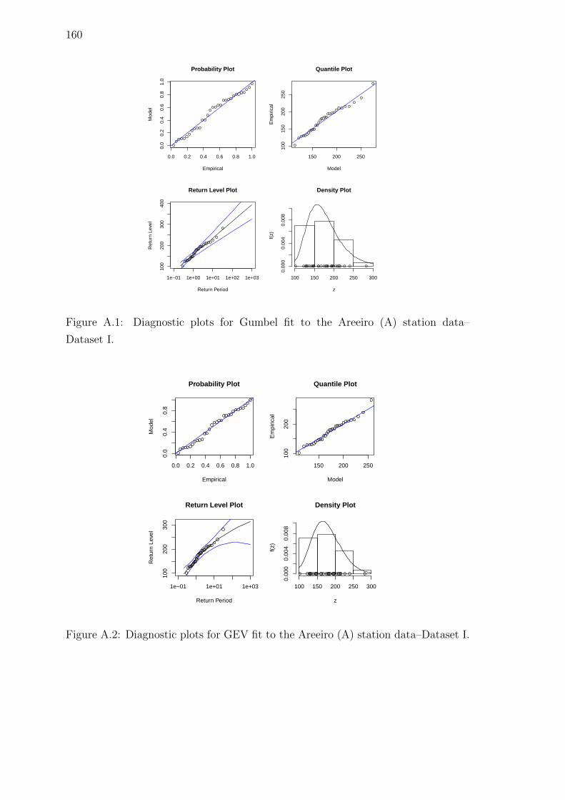
160
0.0 0.2 0.4 0.6 0.8 1.00.
00.
20.
40.
60.
81.
0
Probability Plot
Empirical
Mod
el
150 200 250
100
150
200
250
Quantile Plot
Model
Em
piric
al
1e−01 1e+00 1e+01 1e+02 1e+03
100
200
300
400
Return Period
Ret
urn
Leve
l
Return Level Plot Density Plot
z
f(z)
100 150 200 250 3000.
000
0.00
40.
008
Figure A.1: Diagnostic plots for Gumbel fit to the Areeiro (A) station data–
Dataset I.
0.0 0.2 0.4 0.6 0.8 1.0
0.0
0.4
0.8
Probability Plot
Empirical
Mod
el
150 200 250
100
200
Quantile Plot
Model
Em
piric
al
1e−01 1e+01 1e+03
100
200
300
Return Period
Ret
urn
Leve
l
Return Level Plot Density Plot
z
f(z)
100 150 200 250 300
0.00
00.
004
0.00
8
Figure A.2: Diagnostic plots for GEV fit to the Areeiro (A) station data–Dataset I.

APPENDIX A. DIAGNOSTIC PLOTS FOR ANNUAL MAXIMA 161
0.0 0.2 0.4 0.6 0.8 1.0
0.0
0.4
0.8
Probability Plot
EmpiricalM
odel
100 150 200 250
5010
020
0
Quantile Plot
Model
Em
piric
al
1e−01 1e+01 1e+03
5015
025
035
0
Return Period
Ret
urn
Leve
l
Return Level Plot Density Plot
zf(
z)
50 100 200 300
0.00
00.
004
0.00
8
Figure A.3: Diagnostic plots for Gumbel fit to the Bica da Cana (B) station data–
Dataset I.
0.0 0.2 0.4 0.6 0.8 1.0
0.0
0.2
0.4
0.6
0.8
1.0
Probability Plot
Empirical
Mod
el
100 150 200
5010
015
020
025
0
Quantile Plot
Model
Em
piric
al
1e−01 1e+00 1e+01 1e+02 1e+03
5010
015
020
025
0
Return Period
Ret
urn
Leve
l
Return Level Plot Density Plot
z
f(z)
50 100 150 200 250 300
0.00
00.
004
0.00
8
Figure A.4: Diagnostic plots for GEV fit to the Bica da Cana (B) station data–
Dataset I.
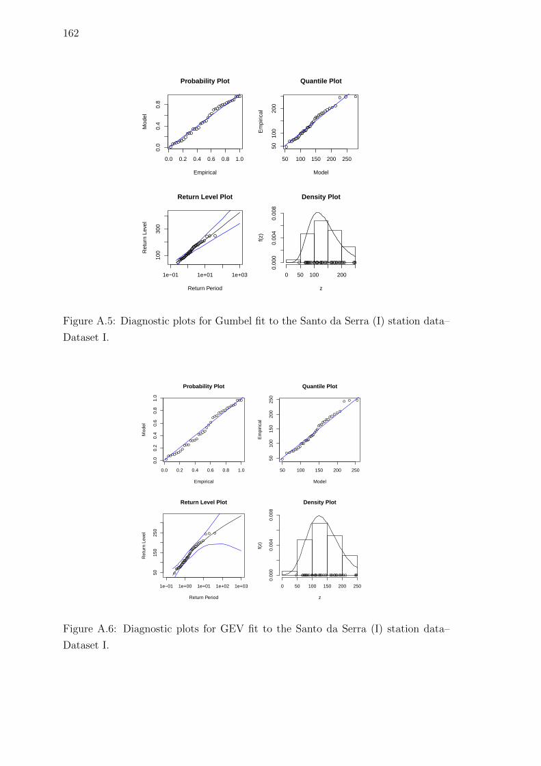
162
0.0 0.2 0.4 0.6 0.8 1.00.
00.
40.
8
Probability Plot
Empirical
Mod
el
50 100 150 200 250
5010
020
0
Quantile Plot
Model
Em
piric
al
1e−01 1e+01 1e+03
100
300
Return Period
Ret
urn
Leve
l
Return Level Plot Density Plot
z
f(z)
0 50 100 2000.
000
0.00
40.
008
Figure A.5: Diagnostic plots for Gumbel fit to the Santo da Serra (I) station data–
Dataset I.
0.0 0.2 0.4 0.6 0.8 1.0
0.0
0.2
0.4
0.6
0.8
1.0
Probability Plot
Empirical
Mod
el
50 100 150 200 250
5010
015
020
025
0
Quantile Plot
Model
Em
piric
al
1e−01 1e+00 1e+01 1e+02 1e+03
5015
025
0
Return Period
Ret
urn
Leve
l
Return Level Plot Density Plot
z
f(z)
0 50 100 150 200 250
0.00
00.
004
0.00
8
Figure A.6: Diagnostic plots for GEV fit to the Santo da Serra (I) station data–
Dataset I.
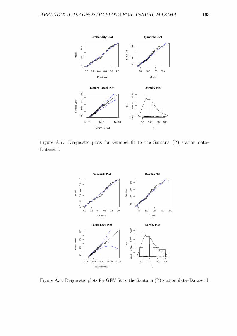
APPENDIX A. DIAGNOSTIC PLOTS FOR ANNUAL MAXIMA 163
0.0 0.2 0.4 0.6 0.8 1.0
0.0
0.4
0.8
Probability Plot
EmpiricalM
odel
50 100 150 200
5010
020
0
Quantile Plot
Model
Em
piric
al
1e−01 1e+01 1e+03
5015
025
035
0
Return Period
Ret
urn
Leve
l
Return Level Plot Density Plot
zf(
z)
50 100 150 200
0.00
00.
006
0.01
2
Figure A.7: Diagnostic plots for Gumbel fit to the Santana (P) station data–
Dataset I.
0.0 0.2 0.4 0.6 0.8 1.0
0.0
0.2
0.4
0.6
0.8
1.0
Probability Plot
Empirical
Mod
el
50 100 150 200 250
5010
015
020
0
Quantile Plot
Model
Em
piric
al
1e−01 1e+00 1e+01 1e+02 1e+03
5015
025
035
0
Return Period
Ret
urn
Leve
l
Return Level Plot Density Plot
z
f(z)
50 100 150 200
0.00
00.
004
0.00
80.
012
Figure A.8: Diagnostic plots for GEV fit to the Santana (P) station data–Dataset I.
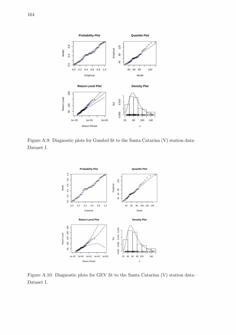
164
0.0 0.2 0.4 0.6 0.8 1.00.
00.
40.
8
Probability Plot
Empirical
Mod
el
40 60 80 120
4080
120
Quantile Plot
Model
Em
piric
al
1e−01 1e+01 1e+03
5010
020
0
Return Period
Ret
urn
Leve
l
Return Level Plot Density Plot
z
f(z)
20 60 100 1400.
000
0.01
0
Figure A.9: Diagnostic plots for Gumbel fit to the Santa Catarina (V) station data–
Dataset I.
0.0 0.2 0.4 0.6 0.8 1.0
0.0
0.2
0.4
0.6
0.8
1.0
Probability Plot
Empirical
Mod
el
40 60 80 100 120 140
4060
8012
0
Quantile Plot
Model
Em
piric
al
1e−01 1e+00 1e+01 1e+02 1e+03
5010
015
020
025
0
Return Period
Ret
urn
Leve
l
Return Level Plot Density Plot
z
f(z)
20 40 60 80 100 140
0.00
00.
005
0.01
00.
015
Figure A.10: Diagnostic plots for GEV fit to the Santa Catarina (V) station data–
Dataset I.
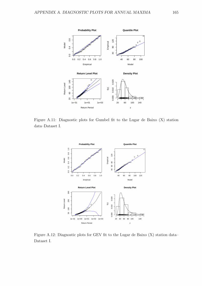
APPENDIX A. DIAGNOSTIC PLOTS FOR ANNUAL MAXIMA 165
0.0 0.2 0.4 0.6 0.8 1.0
0.0
0.4
0.8
Probability Plot
EmpiricalM
odel
40 60 80 100
4080
120
Quantile Plot
Model
Em
piric
al
1e−01 1e+01 1e+03
2060
100
140
Return Period
Ret
urn
Leve
l
Return Level Plot Density Plot
zf(
z)
20 60 100 140
0.00
00.
010
0.02
0
Figure A.11: Diagnostic plots for Gumbel fit to the Lugar de Baixo (X) station
data–Dataset I.
0.0 0.2 0.4 0.6 0.8 1.0
0.0
0.2
0.4
0.6
0.8
1.0
Probability Plot
Empirical
Mod
el
40 60 80 100 120
4060
8012
0
Quantile Plot
Model
Em
piric
al
1e−01 1e+00 1e+01 1e+02 1e+03
5010
020
030
0
Return Period
Ret
urn
Leve
l
Return Level Plot Density Plot
z
f(z)
20 40 60 80 100 140
0.00
00.
010
0.02
0
Figure A.12: Diagnostic plots for GEV fit to the Lugar de Baixo (X) station data–
Dataset I.

166
Appendix B
Likelihood ratio tests’s p–values –
Datasets II and I+II
167
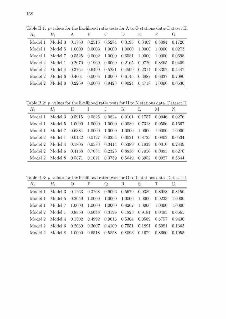
168
Table B.1: p–values for the likelihood ratio tests for A to G stations data–Dataset II.
H0 H1 A B C D E F G
Model 1 Model 3 0.1750 0.2515 0.5284 0.3195 0.3409 0.3084 0.1720
Model 1 Model 5 1.0000 0.0003 1.0000 1.0000 1.0000 1.0000 0.0273
Model 1 Model 7 0.5525 0.0002 1.0000 0.6581 1.0000 1.0000 0.0698
Model 2 Model 1 0.2670 0.1969 0.6069 0.2165 0.0726 0.8865 0.0409
Model 2 Model 4 0.3764 0.6499 0.5231 0.4599 0.2314 0.3302 0.4447
Model 2 Model 6 0.4661 0.0005 1.0000 0.6145 0.3887 0.6037 0.7080
Model 2 Model 8 0.2269 0.0003 0.9423 0.9024 0.4718 1.0000 0.0630
Table B.2: p–values for the likelihood ratio tests for H to N stations data–Dataset II.
H0 H1 H I J K L M N
Model 1 Model 3 0.5915 0.0826 0.0824 0.0101 0.1757 0.0046 0.0276
Model 1 Model 5 1.0000 1.0000 1.0000 0.0089 0.7318 0.0556 0.1667
Model 1 Model 7 0.6384 1.0000 1.0000 1.0000 1.0000 1.0000 1.0000
Model 2 Model 1 0.0132 0.0127 0.0335 0.0021 0.8723 0.0802 0.0534
Model 2 Model 4 0.1806 0.0583 0.3414 0.5389 0.1839 0.0010 0.2849
Model 2 Model 6 0.4158 0.7084 0.2323 0.8836 0.7050 0.0095 0.6276
Model 2 Model 8 0.5871 0.1021 0.3759 0.5649 0.3952 0.0027 0.5644
Table B.3: p–values for the likelihood ratio tests for O to U stations data–Dataset II.
H0 H1 O P Q R S T U
Model 1 Model 3 0.1263 0.3268 0.9096 0.5679 0.0389 0.8988 0.8150
Model 1 Model 5 0.2059 1.0000 1.0000 1.0000 1.0000 0.9233 1.0000
Model 1 Model 7 1.0000 1.0000 1.0000 0.8267 1.0000 1.0000 1.0000
Model 2 Model 1 0.8853 0.6648 0.3196 0.1828 0.9181 0.0495 0.6665
Model 2 Model 4 0.1502 0.4992 0.9613 0.5304 0.0589 0.8757 0.9430
Model 2 Model 6 0.2039 0.3607 0.4109 0.7551 0.1891 0.6081 0.1363
Model 2 Model 8 1.0000 0.6518 0.5858 0.8093 0.1679 0.8660 0.1955

APPENDIX B. LIKELIHOOD RATIO TESTS’S P–VALUES 169
Table B.4: p–values for the likelihood ratio tests for V to Y stations data–Dataset II.
H0 H1 V W X Y
Model 1 Model 3 0.5402 0.0005 0.2161 0.0083
Model 1 Model 5 0.7259 0.0000 0.0288 0.0240
Model 1 Model 7 0.5710 0.5394 0.2261 0.0259
Model 2 Model 1 0.6210 0.0937 0.3635 0.6593
Model 2 Model 4 0.6247 0.2713 0.1249 0.0381
Model 2 Model 6 0.7254 0.9255 0.0211 0.0245
Model 2 Model 8 0.5404 0.2356 0.0690 0.0402
Table B.5: p–values for the likelihood ratio tests for each station data–Dataset I+II.
H0 H1 A B I P U V X
Model 1 Model 3 0.1171 0.1381 0.6048 0.5751 0.1449 0.5922 0.0739
Model 1 Model 5 1.0000 1.0000 1.0000 1.0000 0.4517 0.1089 0.2794
Model 1 Model 7 0.2119 0.4993 1.0000 1.0000 1.0000 0.3368 0.2986
Model 2 Model 1 0.4829 0.0347 0.2232 0.8645 0.4520 0.3125 0.2592
Model 2 Model 4 0.3037 0.3369 0.7167 0.5866 0.1159 0.8393 0.1246
Model 2 Model 6 0.0557 0.0980 0.8155 0.5554 0.4378 0.0620 0.8364
Model 2 Model 8 0.1509 0.0916 0.8332 1.0000 0.2570 0.1486 0.2459

170
Appendix C
Diagnostic plots for annual
maxima – Dataset II (Class 1)
Diagnostic plots for the Gumbel and GEV fits for
the stations with altitude above 900 m
171
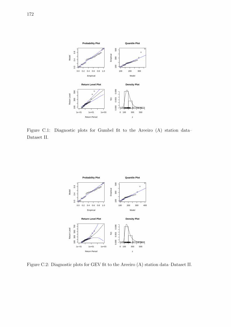
172
0.0 0.2 0.4 0.6 0.8 1.0
0.0
0.4
0.8
Probability Plot
Empirical
Mod
el100 200 300
100
300
500
Quantile Plot
Model
Em
piric
al1e−01 1e+01 1e+03
100
300
500
Return Period
Ret
urn
Leve
l
Return Level Plot Density Plot
z
f(z)
0 100 300 500
0.00
00.
003
0.00
6
Figure C.1: Diagnostic plots for Gumbel fit to the Areeiro (A) station data–
Dataset II.
0.0 0.2 0.4 0.6 0.8 1.0
0.0
0.4
0.8
Probability Plot
Empirical
Mod
el
100 200 300 400
100
300
500
Quantile Plot
Model
Em
piric
al
1e−01 1e+01 1e+03
100
300
500
700
Return Period
Ret
urn
Leve
l
Return Level Plot Density Plot
z
f(z)
0 100 300 500
0.00
00.
003
0.00
6
Figure C.2: Diagnostic plots for GEV fit to the Areeiro (A) station data–Dataset II.

APPENDIX C. DIAGNOSTIC PLOTS FOR ANNUAL MAXIMA 173
0.0 0.2 0.4 0.6 0.8 1.0
0.0
0.4
0.8
Probability Plot
Empirical
Mod
el
100 150 200 250
5010
020
0
Quantile Plot
Model
Em
piric
al
1e−01 1e+01 1e+03
5015
025
035
0
Return Period
Ret
urn
Leve
lReturn Level Plot Density Plot
z
f(z)
50 100 200 300
0.00
00.
006
Figure C.3: Diagnostic plots for Gumbel fit to the Bica da Cana (B) station data–
Dataset II.
0.0 0.2 0.4 0.6 0.8 1.0
0.0
0.4
0.8
Probability Plot
Empirical
Mod
el
100 150 200
5010
020
0
Quantile Plot
Model
Em
piric
al
1e−01 1e+01 1e+03
5015
025
0
Return Period
Ret
urn
Leve
l
Return Level Plot Density Plot
z
f(z)
50 100 200 300
0.00
00.
006
Figure C.4: Diagnostic plots for GEV fit to the Bica da Cana (B) station data–
Dataset II.
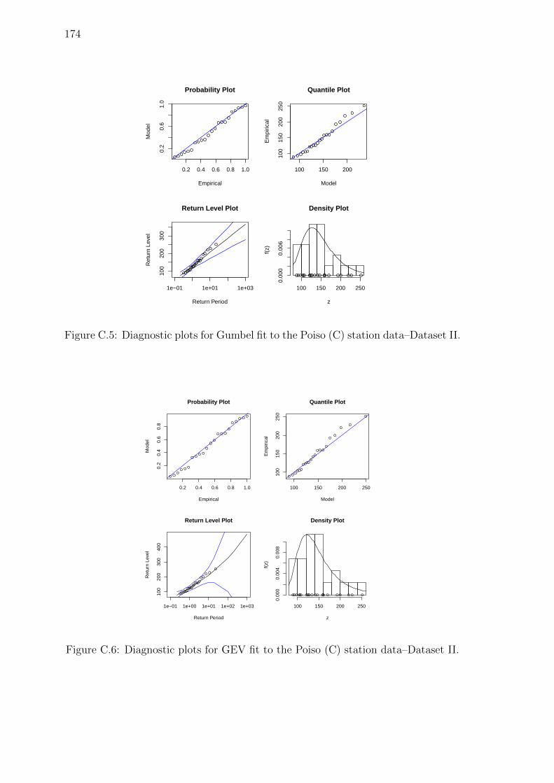
174
0.2 0.4 0.6 0.8 1.0
0.2
0.6
1.0
Probability Plot
Empirical
Mod
el
100 150 200
100
150
200
250
Quantile Plot
Model
Em
piric
al
1e−01 1e+01 1e+03
100
200
300
Return Period
Ret
urn
Leve
l
Return Level Plot Density Plot
z
f(z)
100 150 200 250
0.00
00.
006
Figure C.5: Diagnostic plots for Gumbel fit to the Poiso (C) station data–Dataset II.
0.2 0.4 0.6 0.8 1.0
0.2
0.4
0.6
0.8
Probability Plot
Empirical
Mod
el
100 150 200 250
100
150
200
250
Quantile Plot
Model
Em
piric
al
1e−01 1e+00 1e+01 1e+02 1e+03
100
200
300
400
Return Period
Ret
urn
Leve
l
Return Level Plot Density Plot
z
f(z)
100 150 200 250
0.00
00.
004
0.00
8
Figure C.6: Diagnostic plots for GEV fit to the Poiso (C) station data–Dataset II.
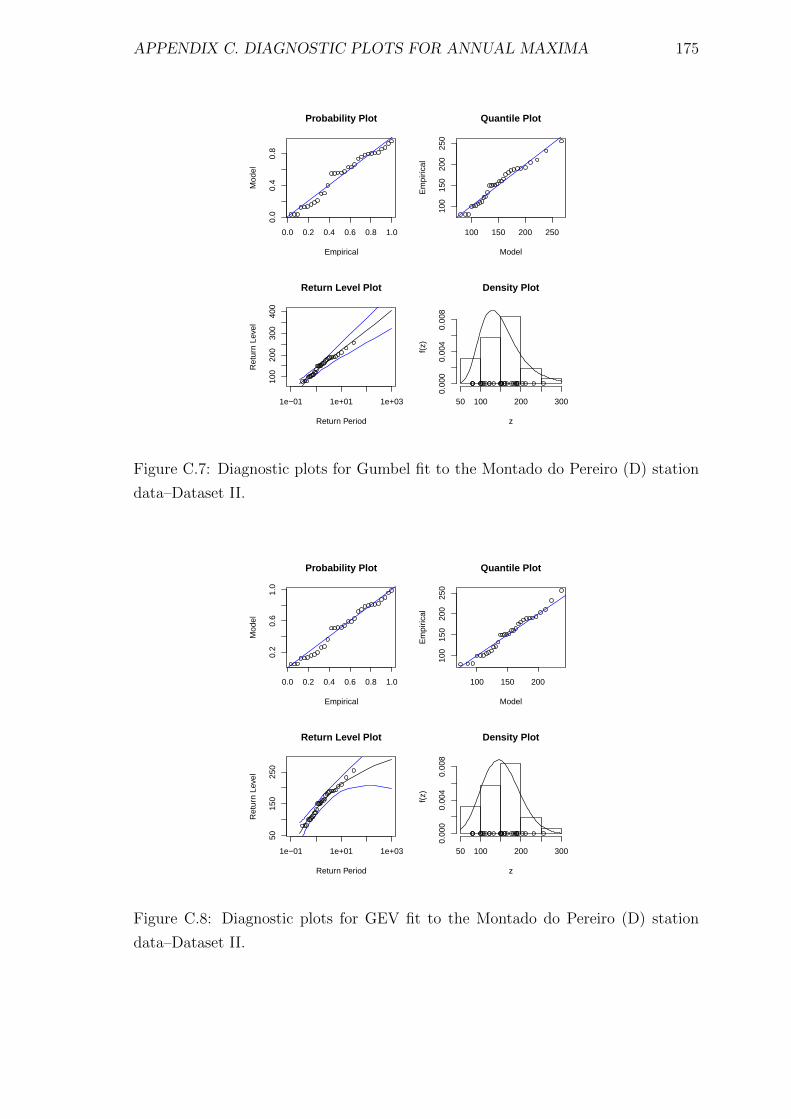
APPENDIX C. DIAGNOSTIC PLOTS FOR ANNUAL MAXIMA 175
0.0 0.2 0.4 0.6 0.8 1.0
0.0
0.4
0.8
Probability Plot
EmpiricalM
odel
100 150 200 250
100
150
200
250
Quantile Plot
Model
Em
piric
al
1e−01 1e+01 1e+03
100
200
300
400
Return Period
Ret
urn
Leve
l
Return Level Plot Density Plot
zf(
z)
50 100 200 300
0.00
00.
004
0.00
8
Figure C.7: Diagnostic plots for Gumbel fit to the Montado do Pereiro (D) station
data–Dataset II.
0.0 0.2 0.4 0.6 0.8 1.0
0.2
0.6
1.0
Probability Plot
Empirical
Mod
el
100 150 200
100
150
200
250
Quantile Plot
Model
Em
piric
al
1e−01 1e+01 1e+03
5015
025
0
Return Period
Ret
urn
Leve
l
Return Level Plot Density Plot
z
f(z)
50 100 200 300
0.00
00.
004
0.00
8
Figure C.8: Diagnostic plots for GEV fit to the Montado do Pereiro (D) station
data–Dataset II.

176
Appendix D
Diagnostic plots for annual
maxima – Dataset II (Class 2)
Diagnostic plots for the Gumbel and GEV fits for
the stations with altitude between 600 and 900 m
177
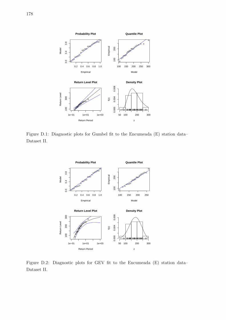
178
0.2 0.4 0.6 0.8 1.00.
00.
40.
8
Probability Plot
Empirical
Mod
el
100 150 200 250 300
100
200
Quantile Plot
Model
Em
piric
al
1e−01 1e+01 1e+03
100
300
Return Period
Ret
urn
Leve
l
Return Level Plot Density Plot
z
f(z)
50 100 200 3000.
000
0.00
40.
008
Figure D.1: Diagnostic plots for Gumbel fit to the Encumeada (E) station data–
Dataset II.
0.2 0.4 0.6 0.8 1.0
0.0
0.4
0.8
Probability Plot
Empirical
Mod
el
100 150 200 250
100
200
Quantile Plot
Model
Em
piric
al
1e−01 1e+01 1e+03
100
200
300
Return Period
Ret
urn
Leve
l
Return Level Plot Density Plot
z
f(z)
50 100 200 300
0.00
00.
004
0.00
8
Figure D.2: Diagnostic plots for GEV fit to the Encumeada (E) station data–
Dataset II.
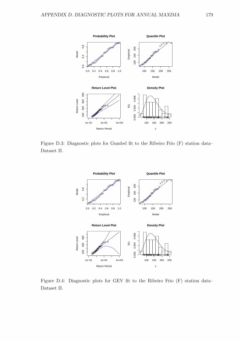
APPENDIX D. DIAGNOSTIC PLOTS FOR ANNUAL MAXIMA 179
0.0 0.2 0.4 0.6 0.8 1.0
0.0
0.4
0.8
Probability Plot
EmpiricalM
odel
100 150 200 250
100
150
200
Quantile Plot
Model
Em
piric
al
1e−01 1e+01 1e+03
100
200
300
400
Return Period
Ret
urn
Leve
l
Return Level Plot Density Plot
zf(
z)
100 150 200 250
0.00
00.
004
0.00
8
Figure D.3: Diagnostic plots for Gumbel fit to the Ribeiro Frio (F) station data–
Dataset II.
0.0 0.2 0.4 0.6 0.8 1.0
0.2
0.6
Probability Plot
Empirical
Mod
el
100 150 200 250
100
150
200
Quantile Plot
Model
Em
piric
al
1e−01 1e+01 1e+03
100
200
300
Return Period
Ret
urn
Leve
l
Return Level Plot Density Plot
z
f(z)
100 150 200 250
0.00
00.
004
0.00
8
Figure D.4: Diagnostic plots for GEV fit to the Ribeiro Frio (F) station data–
Dataset II.
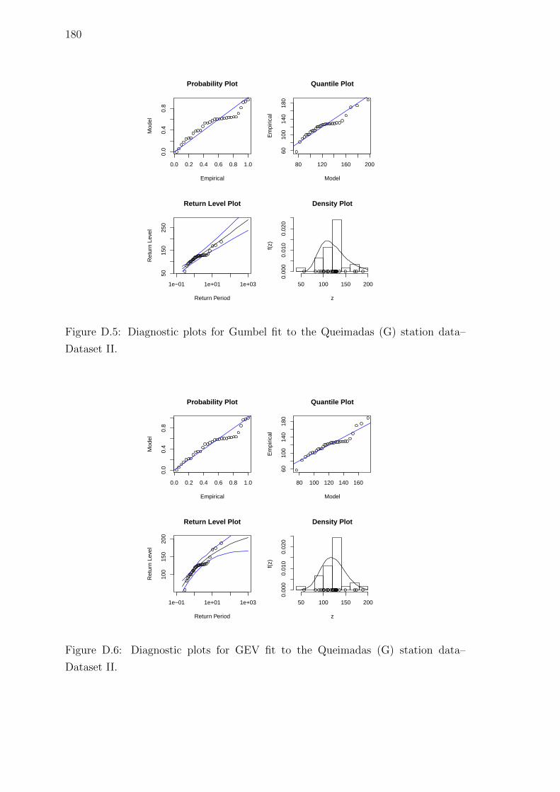
180
0.0 0.2 0.4 0.6 0.8 1.00.
00.
40.
8
Probability Plot
Empirical
Mod
el
80 120 160 200
6010
014
018
0
Quantile Plot
Model
Em
piric
al
1e−01 1e+01 1e+03
5015
025
0
Return Period
Ret
urn
Leve
l
Return Level Plot Density Plot
z
f(z)
50 100 150 2000.
000
0.01
00.
020
Figure D.5: Diagnostic plots for Gumbel fit to the Queimadas (G) station data–
Dataset II.
0.0 0.2 0.4 0.6 0.8 1.0
0.0
0.4
0.8
Probability Plot
Empirical
Mod
el
80 100 120 140 160
6010
014
018
0
Quantile Plot
Model
Em
piric
al
1e−01 1e+01 1e+03
100
150
200
Return Period
Ret
urn
Leve
l
Return Level Plot Density Plot
z
f(z)
50 100 150 200
0.00
00.
010
0.02
0
Figure D.6: Diagnostic plots for GEV fit to the Queimadas (G) station data–
Dataset II.
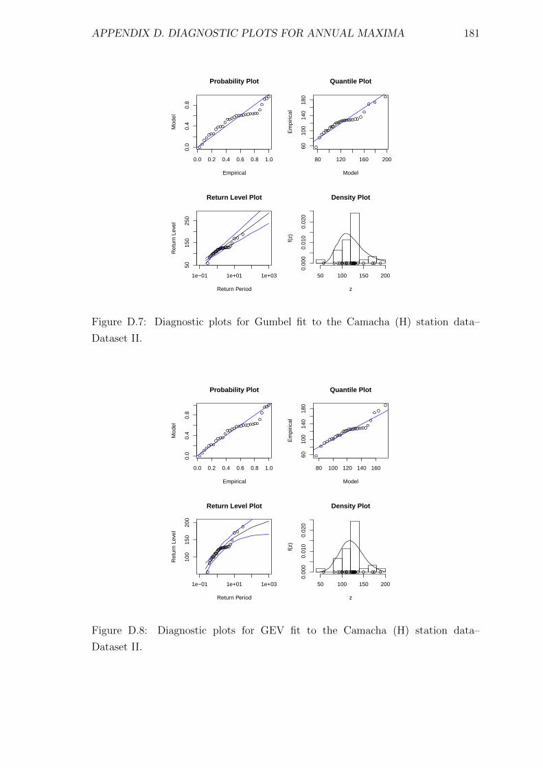
APPENDIX D. DIAGNOSTIC PLOTS FOR ANNUAL MAXIMA 181
0.0 0.2 0.4 0.6 0.8 1.0
0.0
0.4
0.8
Probability Plot
EmpiricalM
odel
80 120 160 200
6010
014
018
0
Quantile Plot
Model
Em
piric
al
1e−01 1e+01 1e+03
5015
025
0
Return Period
Ret
urn
Leve
l
Return Level Plot Density Plot
zf(
z)
50 100 150 200
0.00
00.
010
0.02
0
Figure D.7: Diagnostic plots for Gumbel fit to the Camacha (H) station data–
Dataset II.
0.0 0.2 0.4 0.6 0.8 1.0
0.0
0.4
0.8
Probability Plot
Empirical
Mod
el
80 100 120 140 160
6010
014
018
0
Quantile Plot
Model
Em
piric
al
1e−01 1e+01 1e+03
100
150
200
Return Period
Ret
urn
Leve
l
Return Level Plot Density Plot
z
f(z)
50 100 150 200
0.00
00.
010
0.02
0
Figure D.8: Diagnostic plots for GEV fit to the Camacha (H) station data–
Dataset II.
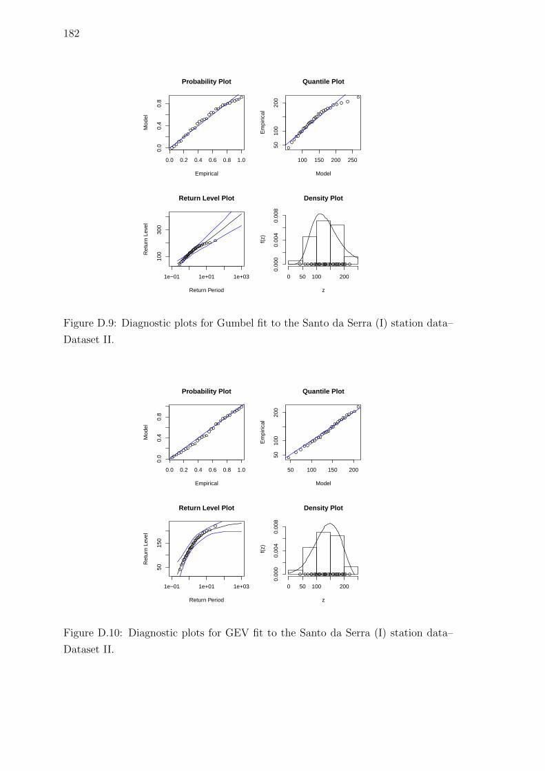
182
0.0 0.2 0.4 0.6 0.8 1.00.
00.
40.
8
Probability Plot
Empirical
Mod
el
100 150 200 250
5010
020
0
Quantile Plot
Model
Em
piric
al
1e−01 1e+01 1e+03
100
300
Return Period
Ret
urn
Leve
l
Return Level Plot Density Plot
z
f(z)
0 50 100 2000.
000
0.00
40.
008
Figure D.9: Diagnostic plots for Gumbel fit to the Santo da Serra (I) station data–
Dataset II.
0.0 0.2 0.4 0.6 0.8 1.0
0.0
0.4
0.8
Probability Plot
Empirical
Mod
el
50 100 150 200
5010
020
0
Quantile Plot
Model
Em
piric
al
1e−01 1e+01 1e+03
5015
0
Return Period
Ret
urn
Leve
l
Return Level Plot Density Plot
z
f(z)
0 50 100 200
0.00
00.
004
0.00
8
Figure D.10: Diagnostic plots for GEV fit to the Santo da Serra (I) station data–
Dataset II.
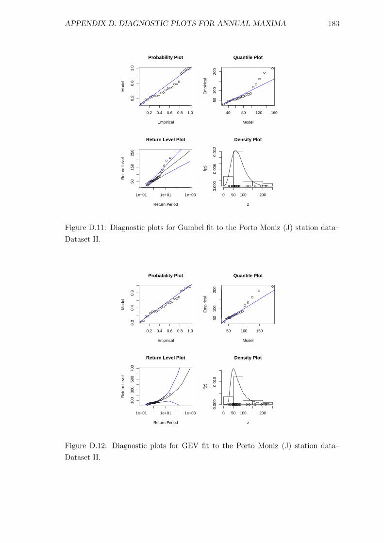
APPENDIX D. DIAGNOSTIC PLOTS FOR ANNUAL MAXIMA 183
0.2 0.4 0.6 0.8 1.0
0.2
0.6
1.0
Probability Plot
EmpiricalM
odel
40 80 120 160
5010
020
0
Quantile Plot
Model
Em
piric
al
1e−01 1e+01 1e+03
5015
025
0
Return Period
Ret
urn
Leve
l
Return Level Plot Density Plot
zf(
z)
0 50 100 200
0.00
00.
006
0.01
2
Figure D.11: Diagnostic plots for Gumbel fit to the Porto Moniz (J) station data–
Dataset II.
0.2 0.4 0.6 0.8 1.0
0.0
0.4
0.8
Probability Plot
Empirical
Mod
el
50 100 150
5010
020
0
Quantile Plot
Model
Em
piric
al
1e−01 1e+01 1e+03
100
300
500
700
Return Period
Ret
urn
Leve
l
Return Level Plot Density Plot
z
f(z)
0 50 100 200
0.00
00.
010
Figure D.12: Diagnostic plots for GEV fit to the Porto Moniz (J) station data–
Dataset II.
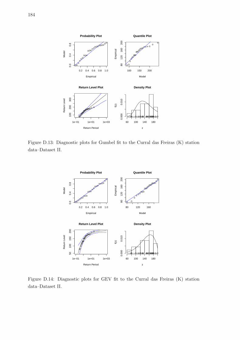
184
0.2 0.4 0.6 0.8 1.00.
00.
40.
8
Probability Plot
Empirical
Mod
el
100 150 200
8012
016
020
0
Quantile Plot
Model
Em
piric
al
1e−01 1e+01 1e+03
100
200
300
Return Period
Ret
urn
Leve
l
Return Level Plot Density Plot
z
f(z)
60 100 140 1800.
000
0.01
0
Figure D.13: Diagnostic plots for Gumbel fit to the Curral das Freiras (K) station
data–Dataset II.
0.2 0.4 0.6 0.8 1.0
0.0
0.4
0.8
Probability Plot
Empirical
Mod
el
80 120 160
8012
016
020
0
Quantile Plot
Model
Em
piric
al
1e−01 1e+01 1e+03
5010
015
020
0
Return Period
Ret
urn
Leve
l
Return Level Plot Density Plot
z
f(z)
60 100 140 180
0.00
00.
010
Figure D.14: Diagnostic plots for GEV fit to the Curral das Freiras (K) station
data–Dataset II.

Appendix E
Diagnostic plots for annual
maxima – Dataset II (Class 3)
Diagnostic plots for the Gumbel and GEV fits for
the stations with altitude between 300 and 600 m
185

186
0.2 0.4 0.6 0.8 1.00.
20.
61.
0
Probability Plot
Empirical
Mod
el
40 60 80 100 120
4060
8012
0
Quantile Plot
Model
Em
piric
al
1e−01 1e+01 1e+03
5010
015
0
Return Period
Ret
urn
Leve
l
Return Level Plot Density Plot
z
f(z)
20 40 60 80 1200.
000
0.01
00.
020
Figure E.1: Diagnostic plots for Gumbel fit to the Ponta do Pargo (L) station data–
Dataset II.
0.2 0.4 0.6 0.8 1.0
0.2
0.6
1.0
Probability Plot
Empirical
Mod
el
40 60 80 100
4060
8012
0
Quantile Plot
Model
Em
piric
al
1e−01 1e+01 1e+03
5010
015
0
Return Period
Ret
urn
Leve
l
Return Level Plot Density Plot
z
f(z)
20 40 60 80 120
0.00
00.
010
0.02
0
Figure E.2: Diagnostic plots for GEV fit to the Ponta do Pargo (L) station data–
Dataset II.
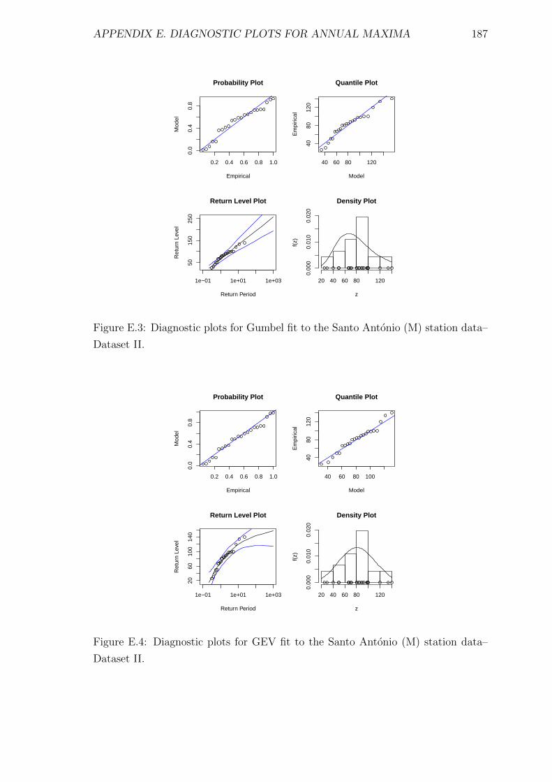
APPENDIX E. DIAGNOSTIC PLOTS FOR ANNUAL MAXIMA 187
0.2 0.4 0.6 0.8 1.0
0.0
0.4
0.8
Probability Plot
EmpiricalM
odel
40 60 80 120
4080
120
Quantile Plot
Model
Em
piric
al
1e−01 1e+01 1e+03
5015
025
0
Return Period
Ret
urn
Leve
l
Return Level Plot Density Plot
zf(
z)
20 40 60 80 120
0.00
00.
010
0.02
0
Figure E.3: Diagnostic plots for Gumbel fit to the Santo Antonio (M) station data–
Dataset II.
0.2 0.4 0.6 0.8 1.0
0.0
0.4
0.8
Probability Plot
Empirical
Mod
el
40 60 80 100
4080
120
Quantile Plot
Model
Em
piric
al
1e−01 1e+01 1e+03
2060
100
140
Return Period
Ret
urn
Leve
l
Return Level Plot Density Plot
z
f(z)
20 40 60 80 120
0.00
00.
010
0.02
0
Figure E.4: Diagnostic plots for GEV fit to the Santo Antonio (M) station data–
Dataset II.
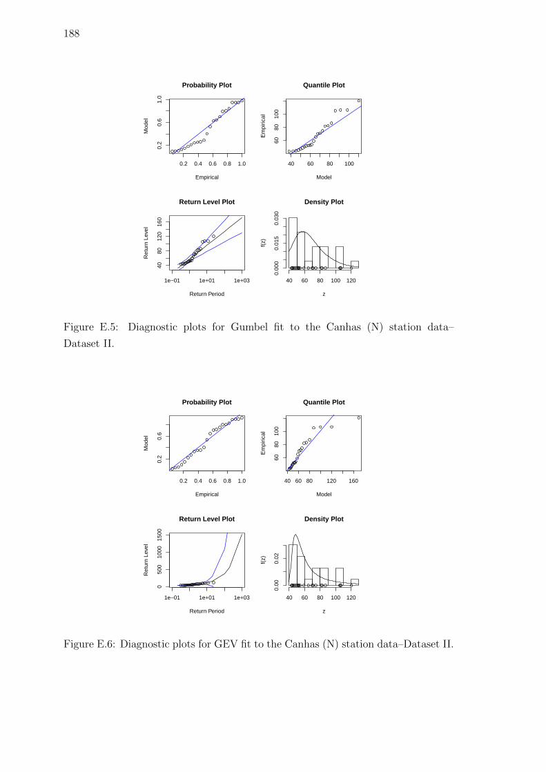
188
0.2 0.4 0.6 0.8 1.00.
20.
61.
0
Probability Plot
Empirical
Mod
el
40 60 80 100
6080
100
Quantile Plot
Model
Em
piric
al
1e−01 1e+01 1e+03
4080
120
160
Return Period
Ret
urn
Leve
l
Return Level Plot Density Plot
z
f(z)
40 60 80 100 1200.
000
0.01
50.
030
Figure E.5: Diagnostic plots for Gumbel fit to the Canhas (N) station data–
Dataset II.
0.2 0.4 0.6 0.8 1.0
0.2
0.6
Probability Plot
Empirical
Mod
el
40 60 80 120 160
6080
100
Quantile Plot
Model
Em
piric
al
1e−01 1e+01 1e+03
050
010
0015
00
Return Period
Ret
urn
Leve
l
Return Level Plot Density Plot
z
f(z)
40 60 80 100 120
0.00
0.02
Figure E.6: Diagnostic plots for GEV fit to the Canhas (N) station data–Dataset II.
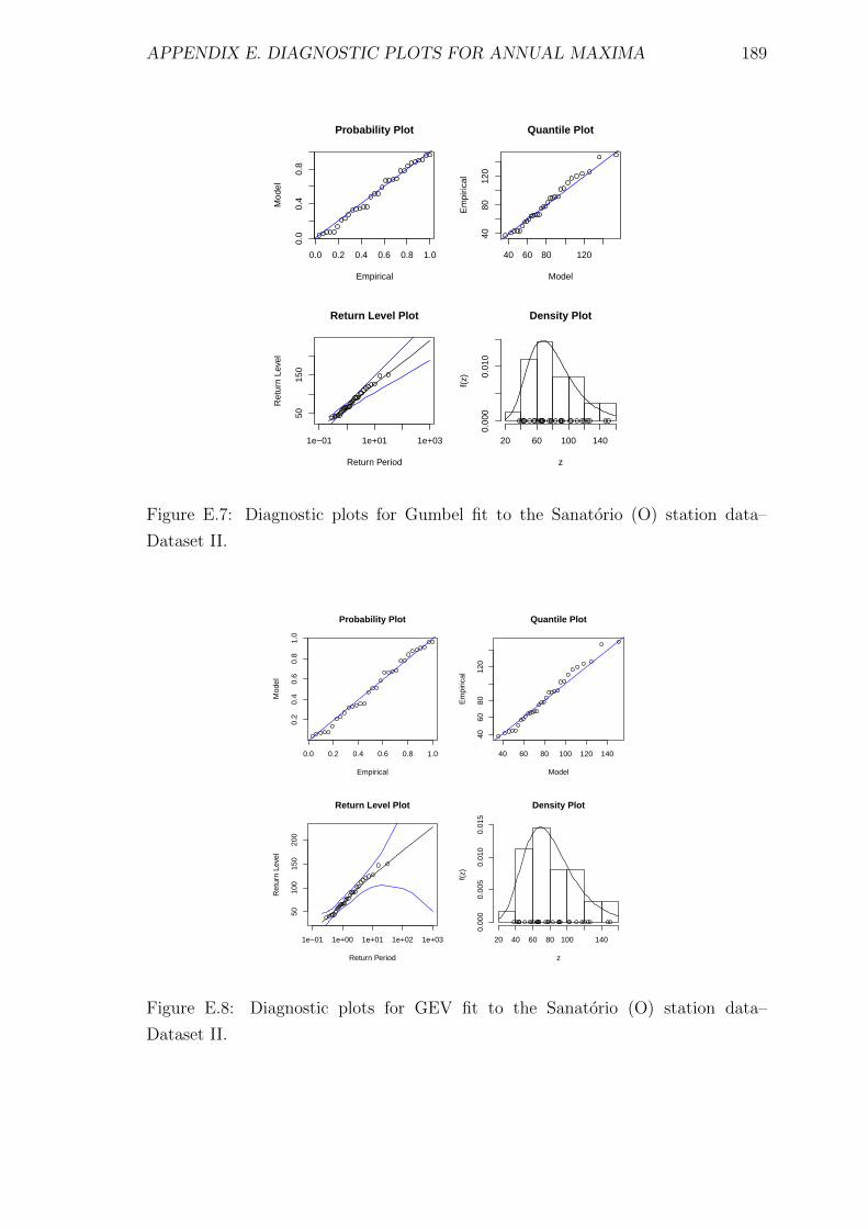
APPENDIX E. DIAGNOSTIC PLOTS FOR ANNUAL MAXIMA 189
0.0 0.2 0.4 0.6 0.8 1.0
0.0
0.4
0.8
Probability Plot
EmpiricalM
odel
40 60 80 120
4080
120
Quantile Plot
Model
Em
piric
al
1e−01 1e+01 1e+03
5015
0
Return Period
Ret
urn
Leve
l
Return Level Plot Density Plot
zf(
z)
20 60 100 140
0.00
00.
010
Figure E.7: Diagnostic plots for Gumbel fit to the Sanatorio (O) station data–
Dataset II.
0.0 0.2 0.4 0.6 0.8 1.0
0.2
0.4
0.6
0.8
1.0
Probability Plot
Empirical
Mod
el
40 60 80 100 120 140
4060
8012
0
Quantile Plot
Model
Em
piric
al
1e−01 1e+00 1e+01 1e+02 1e+03
5010
015
020
0
Return Period
Ret
urn
Leve
l
Return Level Plot Density Plot
z
f(z)
20 40 60 80 100 140
0.00
00.
005
0.01
00.
015
Figure E.8: Diagnostic plots for GEV fit to the Sanatorio (O) station data–
Dataset II.

190
0.0 0.2 0.4 0.6 0.8 1.00.
00.
40.
8
Probability Plot
Empirical
Mod
el
50 100 150 200
5010
015
020
0
Quantile Plot
Model
Em
piric
al
1e−01 1e+01 1e+03
5015
025
0
Return Period
Ret
urn
Leve
l
Return Level Plot Density Plot
z
f(z)
50 100 150 2000.
000
0.00
6
Figure E.9: Diagnostic plots for Gumbel fit to the Santana (P) station data–
Dataset II.
0.0 0.2 0.4 0.6 0.8 1.0
0.0
0.4
0.8
Probability Plot
Empirical
Mod
el
50 100 150 200
5010
015
020
0
Quantile Plot
Model
Em
piric
al
1e−01 1e+01 1e+03
100
300
Return Period
Ret
urn
Leve
l
Return Level Plot Density Plot
z
f(z)
50 100 150 200
0.00
00.
006
Figure E.10: Diagnostic plots for GEV fit to the Santana (P) station data–Dataset II.
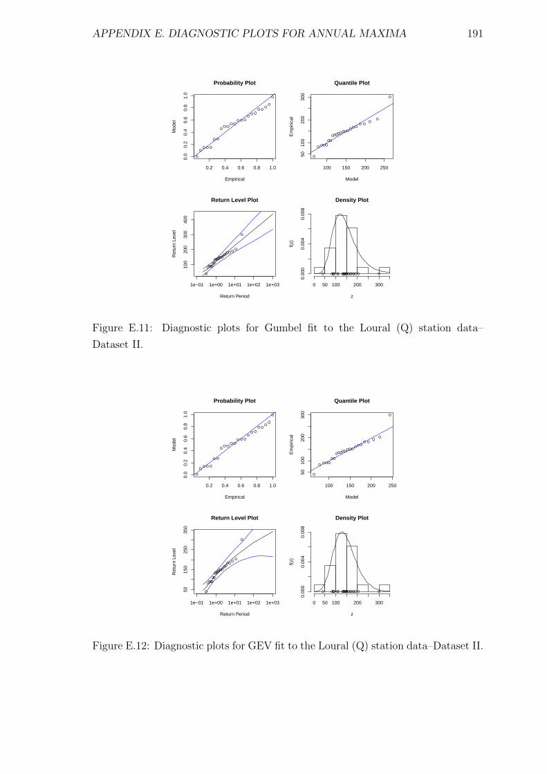
APPENDIX E. DIAGNOSTIC PLOTS FOR ANNUAL MAXIMA 191
0.2 0.4 0.6 0.8 1.0
0.0
0.2
0.4
0.6
0.8
1.0
Probability Plot
EmpiricalM
odel
100 150 200 250
5010
020
030
0
Quantile Plot
Model
Em
piric
al1e−01 1e+00 1e+01 1e+02 1e+03
100
200
300
400
Return Period
Ret
urn
Leve
l
Return Level Plot Density Plot
zf(
z)0 50 100 200 300
0.00
00.
004
0.00
8
Figure E.11: Diagnostic plots for Gumbel fit to the Loural (Q) station data–
Dataset II.
0.2 0.4 0.6 0.8 1.0
0.0
0.2
0.4
0.6
0.8
1.0
Probability Plot
Empirical
Mod
el
100 150 200 250
5010
020
030
0
Quantile Plot
Model
Em
piric
al
1e−01 1e+00 1e+01 1e+02 1e+03
5015
025
035
0
Return Period
Ret
urn
Leve
l
Return Level Plot Density Plot
z
f(z)
0 50 100 200 300
0.00
00.
004
0.00
8
Figure E.12: Diagnostic plots for GEV fit to the Loural (Q) station data–Dataset II.

192

Appendix F
Diagnostic plots for annual
maxima – Dataset II (Class 4)
Diagnostic plots for the Gumbel and GEV fits for
the stations with altitude below 300 m
193
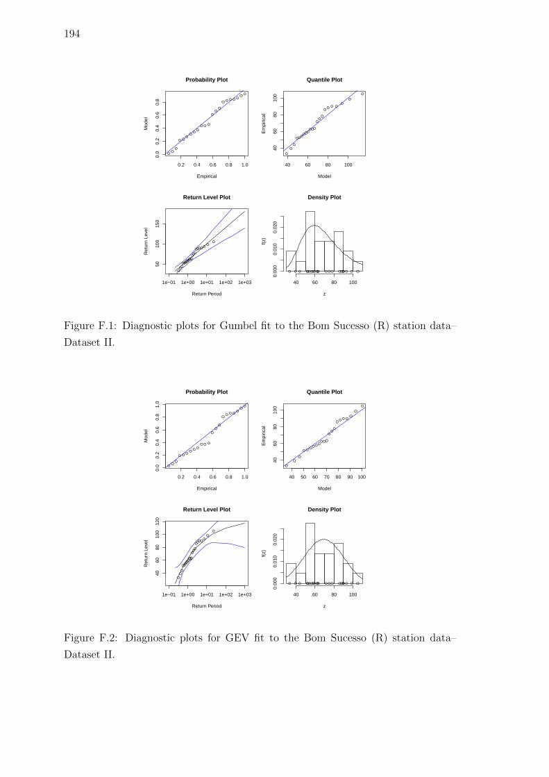
194
0.2 0.4 0.6 0.8 1.0
0.0
0.2
0.4
0.6
0.8
Probability Plot
Empirical
Mod
el
40 60 80 100
4060
8010
0
Quantile Plot
Model
Em
piric
al
1e−01 1e+00 1e+01 1e+02 1e+03
5010
015
0
Return Period
Ret
urn
Leve
l
Return Level Plot Density Plot
z
f(z)
40 60 80 100
0.00
00.
010
0.02
0
Figure F.1: Diagnostic plots for Gumbel fit to the Bom Sucesso (R) station data–
Dataset II.
0.2 0.4 0.6 0.8 1.0
0.0
0.2
0.4
0.6
0.8
1.0
Probability Plot
Empirical
Mod
el
40 50 60 70 80 90 100
4060
8010
0
Quantile Plot
Model
Em
piric
al
1e−01 1e+00 1e+01 1e+02 1e+03
4060
8010
012
0
Return Period
Ret
urn
Leve
l
Return Level Plot Density Plot
z
f(z)
40 60 80 100
0.00
00.
010
0.02
0
Figure F.2: Diagnostic plots for GEV fit to the Bom Sucesso (R) station data–
Dataset II.
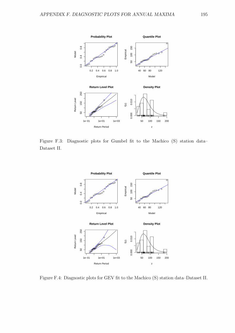
APPENDIX F. DIAGNOSTIC PLOTS FOR ANNUAL MAXIMA 195
0.2 0.4 0.6 0.8 1.0
0.0
0.4
0.8
Probability Plot
EmpiricalM
odel
40 60 80 120
5010
015
0
Quantile Plot
Model
Em
piric
al
1e−01 1e+01 1e+03
5015
025
0
Return Period
Ret
urn
Leve
l
Return Level Plot Density Plot
zf(
z)
50 100 150 200
0.00
00.
010
Figure F.3: Diagnostic plots for Gumbel fit to the Machico (S) station data–
Dataset II.
0.2 0.4 0.6 0.8 1.0
0.0
0.4
0.8
Probability Plot
Empirical
Mod
el
40 60 80 120
5010
015
0
Quantile Plot
Model
Em
piric
al
1e−01 1e+01 1e+03
5015
025
0
Return Period
Ret
urn
Leve
l
Return Level Plot Density Plot
z
f(z)
50 100 150 200
0.00
00.
010
Figure F.4: Diagnostic plots for GEV fit to the Machico (S) station data–Dataset II.

196
0.0 0.2 0.4 0.6 0.8 1.00.
00.
40.
8
Probability Plot
Empirical
Mod
el
50 100 150
5015
025
0
Quantile Plot
Model
Em
piric
al
1e−01 1e+01 1e+03
5015
025
0
Return Period
Ret
urn
Leve
l
Return Level Plot Density Plot
z
f(z)
0 50 150 250 3500.
000
0.00
60.
012
Figure F.5: Diagnostic plots for Gumbel fit to the Ponta Delgada (T) station data–
Dataset II.
0.0 0.2 0.4 0.6 0.8 1.0
0.0
0.4
0.8
Probability Plot
Empirical
Mod
el
50 100 150 200
5015
025
0
Quantile Plot
Model
Em
piric
al
1e−01 1e+01 1e+03
100
300
500
Return Period
Ret
urn
Leve
l
Return Level Plot Density Plot
z
f(z)
0 50 150 250 350
0.00
00.
006
0.01
2
Figure F.6: Diagnostic plots for GEV fit to the Ponta Delgada (T) station data–
Dataset II.
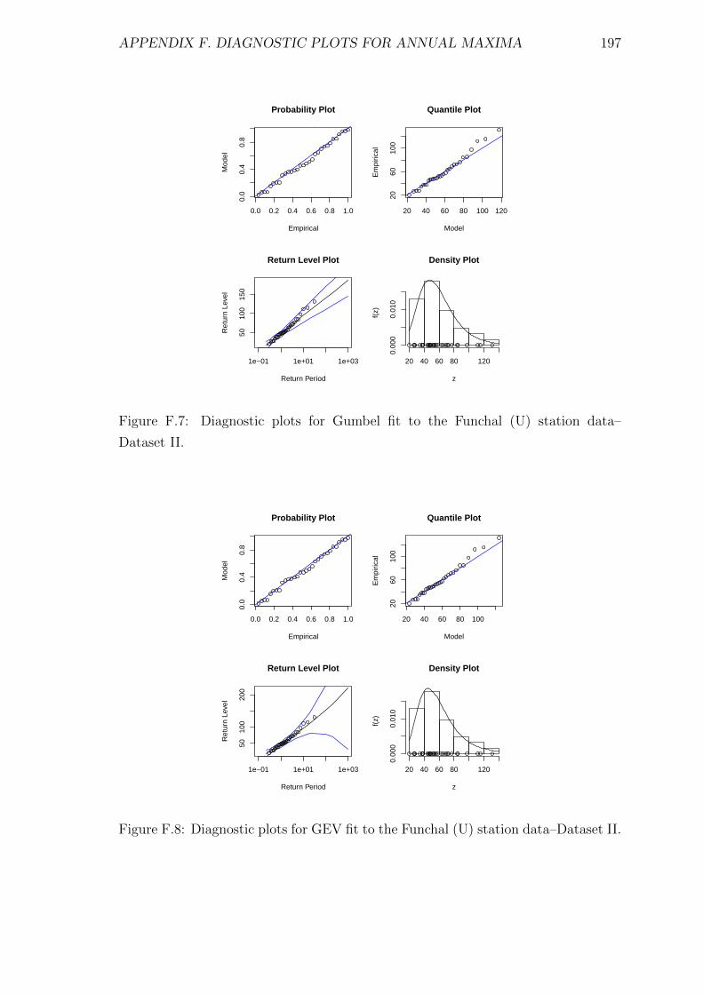
APPENDIX F. DIAGNOSTIC PLOTS FOR ANNUAL MAXIMA 197
0.0 0.2 0.4 0.6 0.8 1.0
0.0
0.4
0.8
Probability Plot
EmpiricalM
odel
20 40 60 80 100 120
2060
100
Quantile Plot
Model
Em
piric
al
1e−01 1e+01 1e+03
5010
015
0
Return Period
Ret
urn
Leve
l
Return Level Plot Density Plot
zf(
z)
20 40 60 80 120
0.00
00.
010
Figure F.7: Diagnostic plots for Gumbel fit to the Funchal (U) station data–
Dataset II.
0.0 0.2 0.4 0.6 0.8 1.0
0.0
0.4
0.8
Probability Plot
Empirical
Mod
el
20 40 60 80 100
2060
100
Quantile Plot
Model
Em
piric
al
1e−01 1e+01 1e+03
5010
020
0
Return Period
Ret
urn
Leve
l
Return Level Plot Density Plot
z
f(z)
20 40 60 80 120
0.00
00.
010
Figure F.8: Diagnostic plots for GEV fit to the Funchal (U) station data–Dataset II.
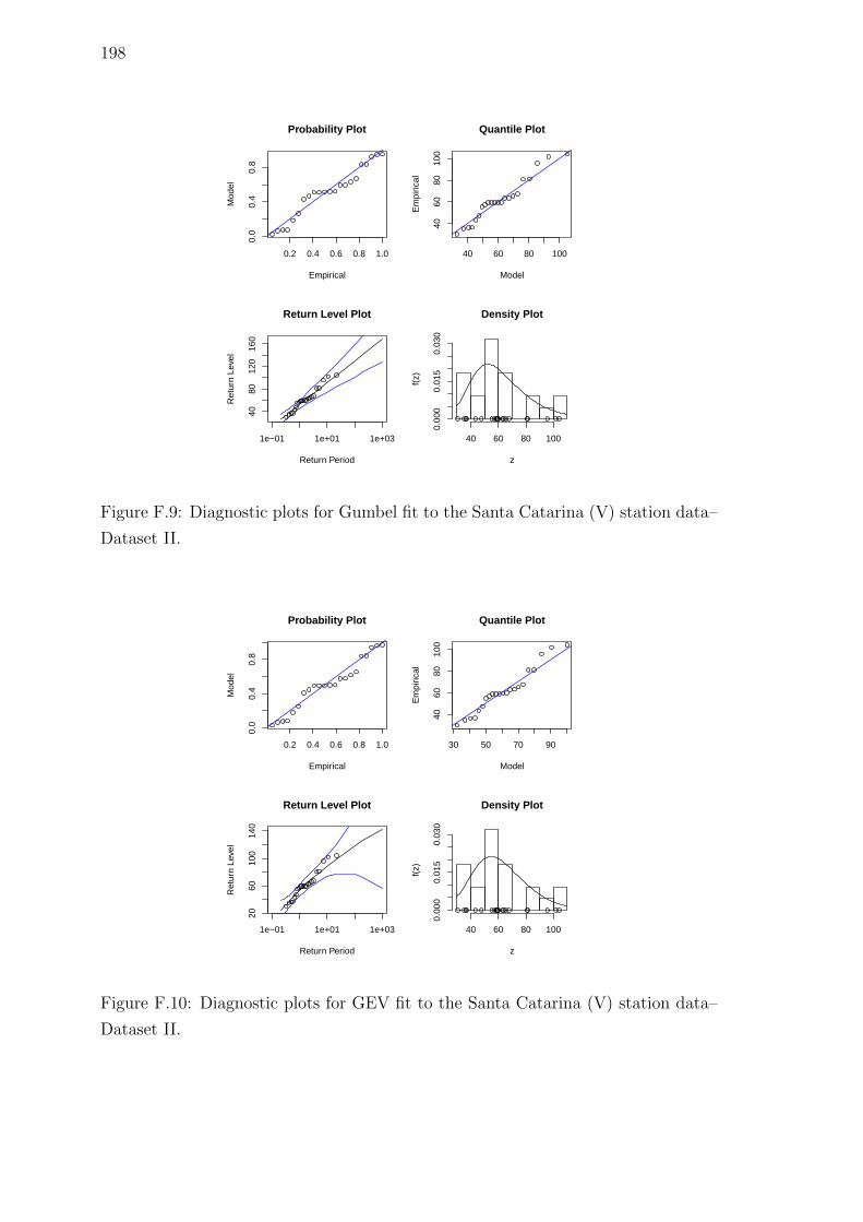
198
0.2 0.4 0.6 0.8 1.00.
00.
40.
8
Probability Plot
Empirical
Mod
el
40 60 80 100
4060
8010
0
Quantile Plot
Model
Em
piric
al
1e−01 1e+01 1e+03
4080
120
160
Return Period
Ret
urn
Leve
l
Return Level Plot Density Plot
z
f(z)
40 60 80 1000.
000
0.01
50.
030
Figure F.9: Diagnostic plots for Gumbel fit to the Santa Catarina (V) station data–
Dataset II.
0.2 0.4 0.6 0.8 1.0
0.0
0.4
0.8
Probability Plot
Empirical
Mod
el
30 50 70 90
4060
8010
0
Quantile Plot
Model
Em
piric
al
1e−01 1e+01 1e+03
2060
100
140
Return Period
Ret
urn
Leve
l
Return Level Plot Density Plot
z
f(z)
40 60 80 100
0.00
00.
015
0.03
0
Figure F.10: Diagnostic plots for GEV fit to the Santa Catarina (V) station data–
Dataset II.
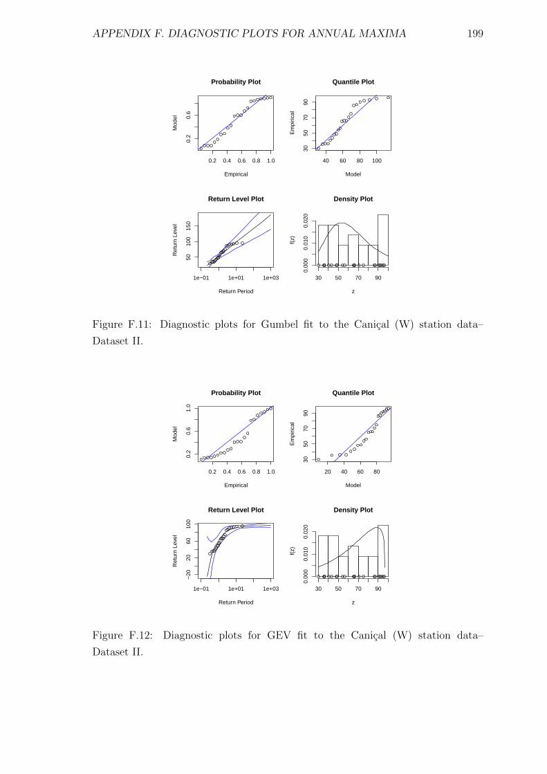
APPENDIX F. DIAGNOSTIC PLOTS FOR ANNUAL MAXIMA 199
0.2 0.4 0.6 0.8 1.0
0.2
0.6
Probability Plot
EmpiricalM
odel
40 60 80 100
3050
7090
Quantile Plot
Model
Em
piric
al
1e−01 1e+01 1e+03
5010
015
0
Return Period
Ret
urn
Leve
l
Return Level Plot Density Plot
zf(
z)
30 50 70 90
0.00
00.
010
0.02
0
Figure F.11: Diagnostic plots for Gumbel fit to the Canical (W) station data–
Dataset II.
0.2 0.4 0.6 0.8 1.0
0.2
0.6
1.0
Probability Plot
Empirical
Mod
el
20 40 60 80
3050
7090
Quantile Plot
Model
Em
piric
al
1e−01 1e+01 1e+03
−20
2060
100
Return Period
Ret
urn
Leve
l
Return Level Plot Density Plot
z
f(z)
30 50 70 90
0.00
00.
010
0.02
0
Figure F.12: Diagnostic plots for GEV fit to the Canical (W) station data–
Dataset II.
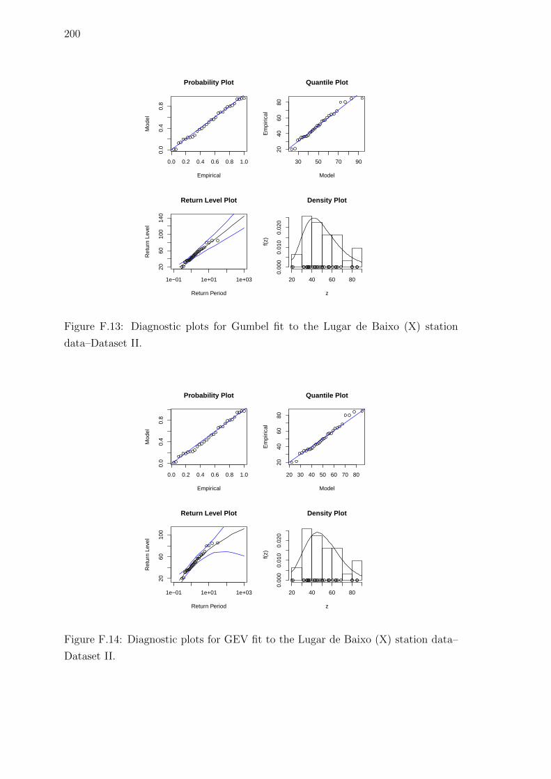
200
0.0 0.2 0.4 0.6 0.8 1.00.
00.
40.
8
Probability Plot
Empirical
Mod
el
30 50 70 90
2040
6080
Quantile Plot
Model
Em
piric
al
1e−01 1e+01 1e+03
2060
100
140
Return Period
Ret
urn
Leve
l
Return Level Plot Density Plot
z
f(z)
20 40 60 800.
000
0.01
00.
020
Figure F.13: Diagnostic plots for Gumbel fit to the Lugar de Baixo (X) station
data–Dataset II.
0.0 0.2 0.4 0.6 0.8 1.0
0.0
0.4
0.8
Probability Plot
Empirical
Mod
el
20 30 40 50 60 70 80
2040
6080
Quantile Plot
Model
Em
piric
al
1e−01 1e+01 1e+03
2060
100
Return Period
Ret
urn
Leve
l
Return Level Plot Density Plot
z
f(z)
20 40 60 80
0.00
00.
010
0.02
0
Figure F.14: Diagnostic plots for GEV fit to the Lugar de Baixo (X) station data–
Dataset II.
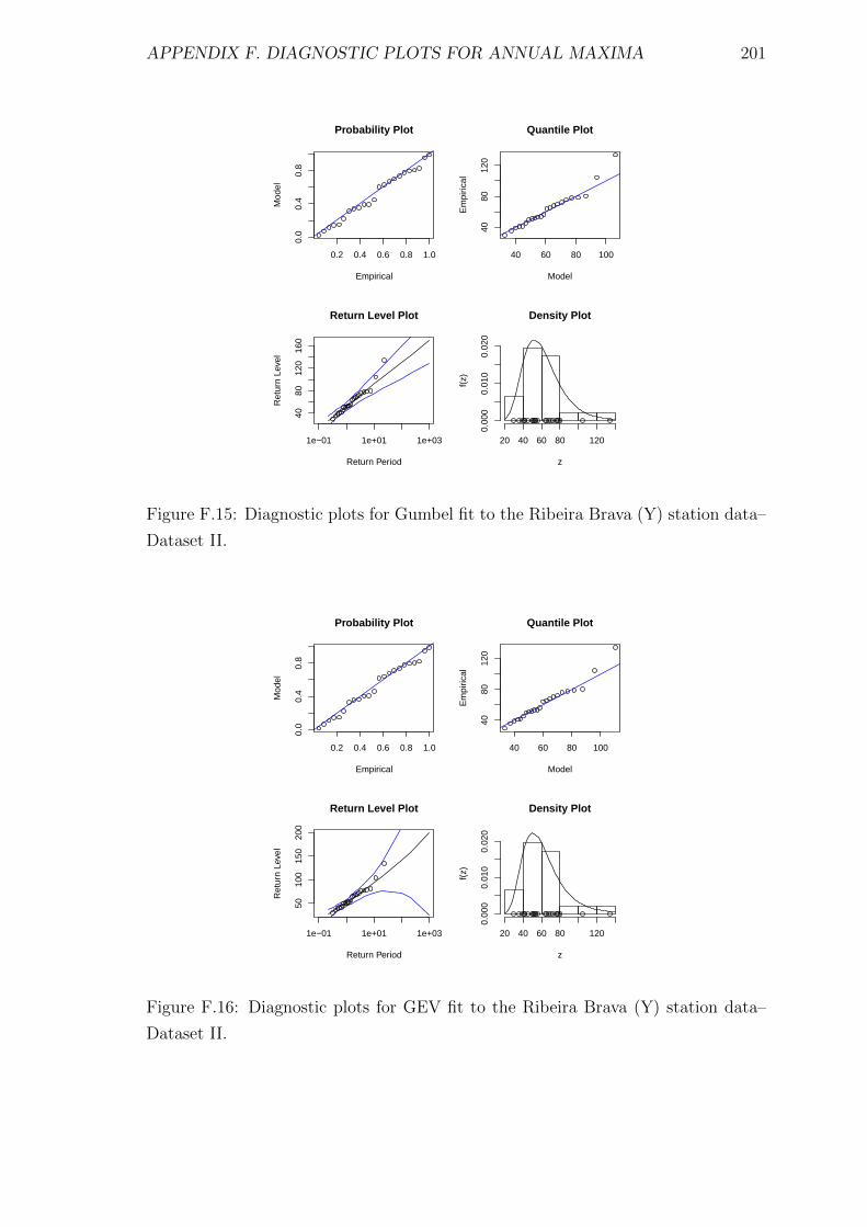
APPENDIX F. DIAGNOSTIC PLOTS FOR ANNUAL MAXIMA 201
0.2 0.4 0.6 0.8 1.0
0.0
0.4
0.8
Probability Plot
EmpiricalM
odel
40 60 80 100
4080
120
Quantile Plot
Model
Em
piric
al
1e−01 1e+01 1e+03
4080
120
160
Return Period
Ret
urn
Leve
l
Return Level Plot Density Plot
zf(
z)
20 40 60 80 120
0.00
00.
010
0.02
0
Figure F.15: Diagnostic plots for Gumbel fit to the Ribeira Brava (Y) station data–
Dataset II.
0.2 0.4 0.6 0.8 1.0
0.0
0.4
0.8
Probability Plot
Empirical
Mod
el
40 60 80 100
4080
120
Quantile Plot
Model
Em
piric
al
1e−01 1e+01 1e+03
5010
015
020
0
Return Period
Ret
urn
Leve
l
Return Level Plot Density Plot
z
f(z)
20 40 60 80 120
0.00
00.
010
0.02
0
Figure F.16: Diagnostic plots for GEV fit to the Ribeira Brava (Y) station data–
Dataset II.

202
Appendix G
Diagnostic plots for annual
maxima – Dataset I+II
Diagnostic plots for the Gumbel and GEV fits
203
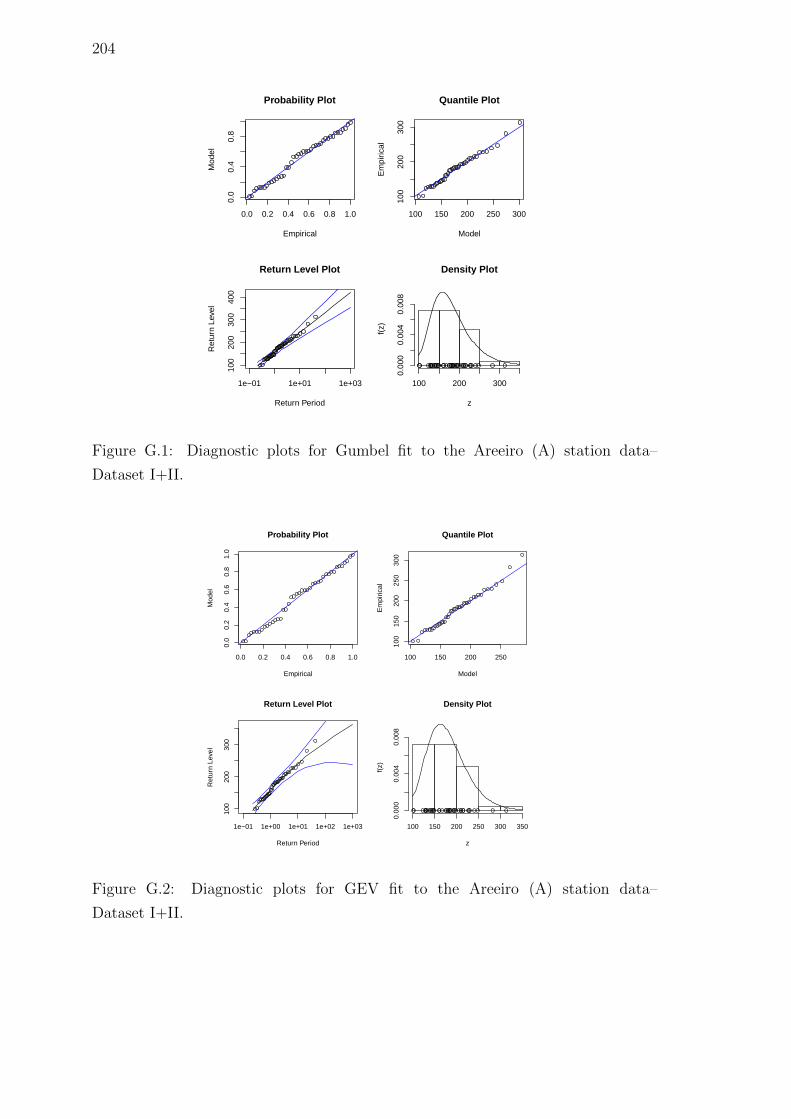
204
0.0 0.2 0.4 0.6 0.8 1.0
0.0
0.4
0.8
Probability Plot
Empirical
Mod
el100 150 200 250 300
100
200
300
Quantile Plot
Model
Em
piric
al1e−01 1e+01 1e+03
100
200
300
400
Return Period
Ret
urn
Leve
l
Return Level Plot Density Plot
z
f(z)
100 200 300
0.00
00.
004
0.00
8
Figure G.1: Diagnostic plots for Gumbel fit to the Areeiro (A) station data–
Dataset I+II.
0.0 0.2 0.4 0.6 0.8 1.0
0.0
0.2
0.4
0.6
0.8
1.0
Probability Plot
Empirical
Mod
el
100 150 200 250
100
150
200
250
300
Quantile Plot
Model
Em
piric
al
1e−01 1e+00 1e+01 1e+02 1e+03
100
200
300
Return Period
Ret
urn
Leve
l
Return Level Plot Density Plot
z
f(z)
100 150 200 250 300 350
0.00
00.
004
0.00
8
Figure G.2: Diagnostic plots for GEV fit to the Areeiro (A) station data–
Dataset I+II.

APPENDIX G. DIAGNOSTIC PLOTS FOR ANNUAL MAXIMA 205
0.0 0.2 0.4 0.6 0.8 1.0
0.0
0.4
0.8
Probability Plot
EmpiricalM
odel
100 150 200 250
5010
020
0
Quantile Plot
Model
Em
piric
al
1e−01 1e+01 1e+03
5015
025
035
0
Return Period
Ret
urn
Leve
l
Return Level Plot Density Plot
zf(
z)
50 100 200 300
0.00
00.
004
0.00
8
Figure G.3: Diagnostic plots for Gumbel fit to the Bica da Cana (B) station data–
Dataset I+II.
0.0 0.2 0.4 0.6 0.8 1.0
0.0
0.4
0.8
Probability Plot
Empirical
Mod
el
100 150 200
5010
020
0
Quantile Plot
Model
Em
piric
al
1e−01 1e+01 1e+03
5015
025
0
Return Period
Ret
urn
Leve
l
Return Level Plot Density Plot
z
f(z)
50 100 200 300
0.00
00.
004
0.00
8
Figure G.4: Diagnostic plots for GEV fit to the Bica da Cana (B) station data–
Dataset I+II.
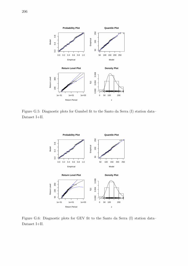
206
0.0 0.2 0.4 0.6 0.8 1.00.
00.
40.
8
Probability Plot
Empirical
Mod
el
50 100 150 200 250
5015
025
0
Quantile Plot
Model
Em
piric
al
1e−01 1e+01 1e+03
100
300
Return Period
Ret
urn
Leve
l
Return Level Plot Density Plot
z
f(z)
0 50 100 2000.
000
0.00
40.
008
Figure G.5: Diagnostic plots for Gumbel fit to the Santo da Serra (I) station data–
Dataset I+II.
0.0 0.2 0.4 0.6 0.8 1.0
0.0
0.4
0.8
Probability Plot
Empirical
Mod
el
50 100 150 200 250
5015
025
0
Quantile Plot
Model
Em
piric
al
1e−01 1e+01 1e+03
5015
025
0
Return Period
Ret
urn
Leve
l
Return Level Plot Density Plot
z
f(z)
0 50 100 200
0.00
00.
004
0.00
8
Figure G.6: Diagnostic plots for GEV fit to the Santo da Serra (I) station data–
Dataset I+II.
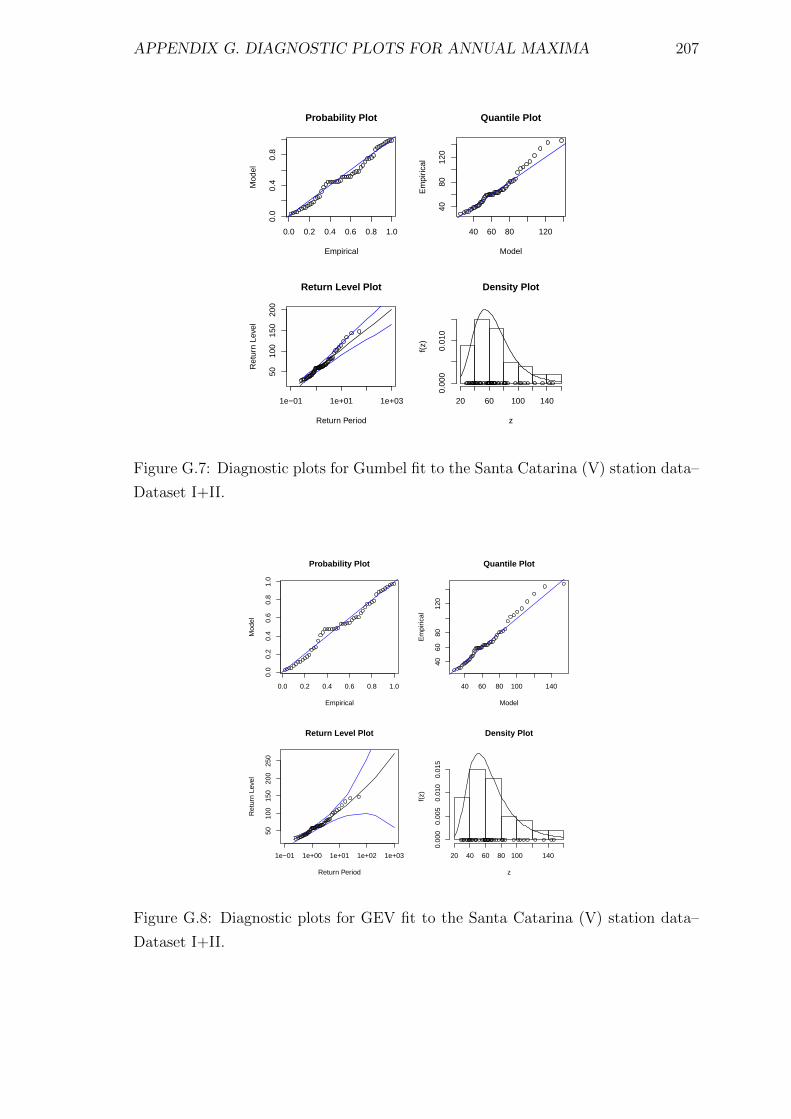
APPENDIX G. DIAGNOSTIC PLOTS FOR ANNUAL MAXIMA 207
0.0 0.2 0.4 0.6 0.8 1.0
0.0
0.4
0.8
Probability Plot
EmpiricalM
odel
40 60 80 120
4080
120
Quantile Plot
Model
Em
piric
al
1e−01 1e+01 1e+03
5010
015
020
0
Return Period
Ret
urn
Leve
l
Return Level Plot Density Plot
zf(
z)
20 60 100 140
0.00
00.
010
Figure G.7: Diagnostic plots for Gumbel fit to the Santa Catarina (V) station data–
Dataset I+II.
0.0 0.2 0.4 0.6 0.8 1.0
0.0
0.2
0.4
0.6
0.8
1.0
Probability Plot
Empirical
Mod
el
40 60 80 100 140
4060
8012
0
Quantile Plot
Model
Em
piric
al
1e−01 1e+00 1e+01 1e+02 1e+03
5010
015
020
025
0
Return Period
Ret
urn
Leve
l
Return Level Plot Density Plot
z
f(z)
20 40 60 80 100 140
0.00
00.
005
0.01
00.
015
Figure G.8: Diagnostic plots for GEV fit to the Santa Catarina (V) station data–
Dataset I+II.
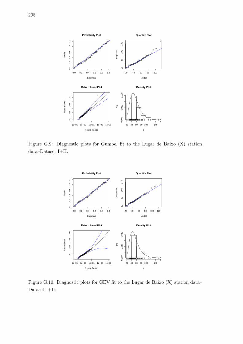
208
0.0 0.2 0.4 0.6 0.8 1.0
0.0
0.2
0.4
0.6
0.8
1.0
Probability Plot
Empirical
Mod
el
20 40 60 80 100
2060
100
140
Quantile Plot
Model
Em
piric
al
1e−01 1e+00 1e+01 1e+02 1e+03
2060
100
140
Return Period
Ret
urn
Leve
l
Return Level Plot Density Plot
z
f(z)
20 40 60 80 100 140
0.00
00.
010
0.02
0
Figure G.9: Diagnostic plots for Gumbel fit to the Lugar de Baixo (X) station
data–Dataset I+II.
0.0 0.2 0.4 0.6 0.8 1.0
0.0
0.2
0.4
0.6
0.8
1.0
Probability Plot
Empirical
Mod
el
20 40 60 80 100 120
2060
100
140
Quantile Plot
Model
Em
piric
al
1e−01 1e+00 1e+01 1e+02 1e+03
5010
015
020
0
Return Period
Ret
urn
Leve
l
Return Level Plot Density Plot
z
f(z)
20 40 60 80 100 140
0.00
00.
010
0.02
0
Figure G.10: Diagnostic plots for GEV fit to the Lugar de Baixo (X) station data–
Dataset I+II.
Appendix H
Threshold choice plots – Dataset
IV (Class 1)
Mean residual and parameter stability plots for the
stations with altitude above 900 m
209

210
0 50 100 150 200
010
2030
4050
Mean Residual Life Plot
Threshold
Mea
n E
xces
s
Figure H.1: Mean residual plot for the Bica da Cana (B) station data.
0 50 100 150 200
−20
020
0
Threshold
Mod
ified
Sca
le
0 50 100 150 200
−2.
00.
0
Threshold
Sha
pe
Figure H.2: Parameter stability plots for the Bica da Cana (B) station data.

APPENDIX H. THRESHOLD CHOICE PLOTS – DATASET IV (CLASS 1) 211
0 50 100 150 200
1020
3040
5060
Mean Residual Life Plot
Threshold
Mea
n E
xces
s
Figure H.3: Mean residual plot for the Poiso (C) station data.
0 50 100 150
−10
020
0
Threshold
Mod
ified
Sca
le
0 50 100 150
−1.
50.
01.
0
Threshold
Sha
pe
Figure H.4: Parameter stability plots for the Poiso (C) station data.
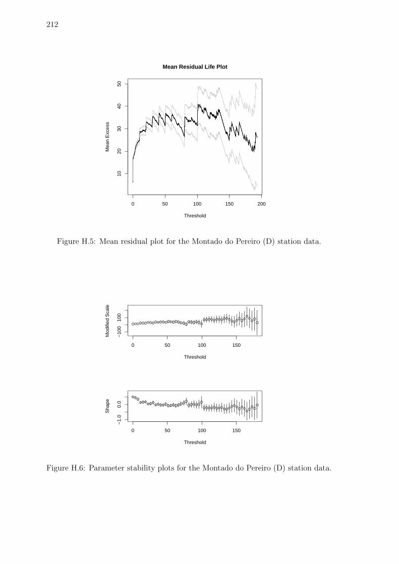
212
0 50 100 150 200
1020
3040
50
Mean Residual Life Plot
Threshold
Mea
n E
xces
s
Figure H.5: Mean residual plot for the Montado do Pereiro (D) station data.
0 50 100 150
−10
010
0
Threshold
Mod
ified
Sca
le
0 50 100 150
−1.
00.
0
Threshold
Sha
pe
Figure H.6: Parameter stability plots for the Montado do Pereiro (D) station data.
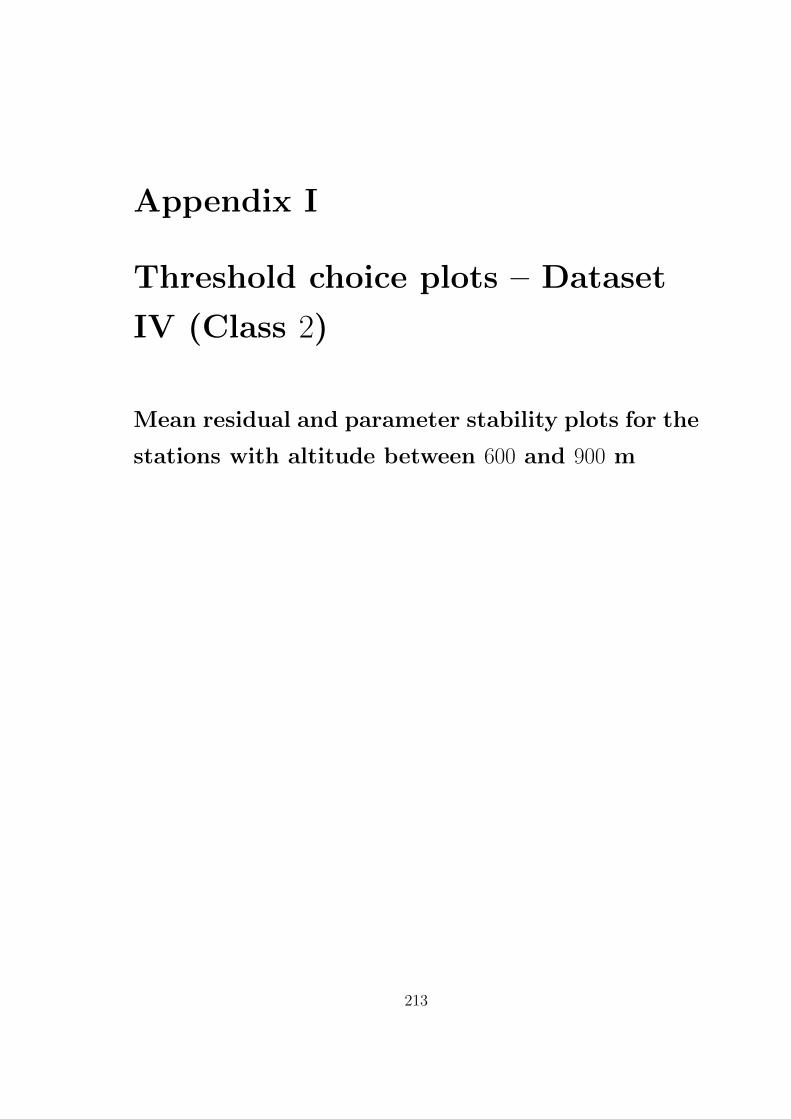
Appendix I
Threshold choice plots – Dataset
IV (Class 2)
Mean residual and parameter stability plots for the
stations with altitude between 600 and 900 m
213
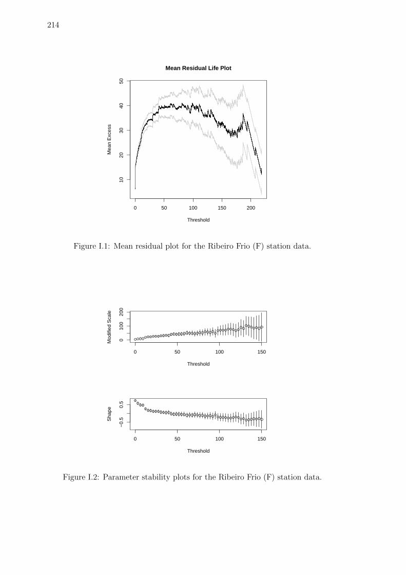
214
0 50 100 150 200
1020
3040
50
Mean Residual Life Plot
Threshold
Mea
n E
xces
s
Figure I.1: Mean residual plot for the Ribeiro Frio (F) station data.
0 50 100 150
010
020
0
Threshold
Mod
ified
Sca
le
0 50 100 150
−0.
50.
5
Threshold
Sha
pe
Figure I.2: Parameter stability plots for the Ribeiro Frio (F) station data.
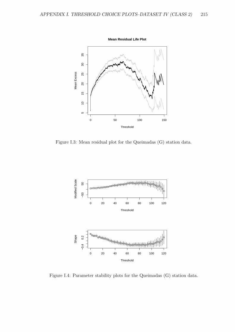
APPENDIX I. THRESHOLD CHOICE PLOTS–DATASET IV (CLASS 2) 215
0 50 100 150
510
1520
2530
35
Mean Residual Life Plot
Threshold
Mea
n E
xces
s
Figure I.3: Mean residual plot for the Queimadas (G) station data.
0 20 40 60 80 100 120
−50
50
Threshold
Mod
ified
Sca
le
0 20 40 60 80 100 120
−0.
40.
2
Threshold
Sha
pe
Figure I.4: Parameter stability plots for the Queimadas (G) station data.

216
0 50 100 150
010
2030
40
Mean Residual Life Plot
Threshold
Mea
n E
xces
s
Figure I.5: Mean residual plot for the Camacha (H) station data.
0 20 40 60 80 100 120
010
020
0
Threshold
Mod
ified
Sca
le
0 20 40 60 80 100 120
−1.
00.
0
Threshold
Sha
pe
Figure I.6: Parameter stability plots for the Camacha (H) station data.
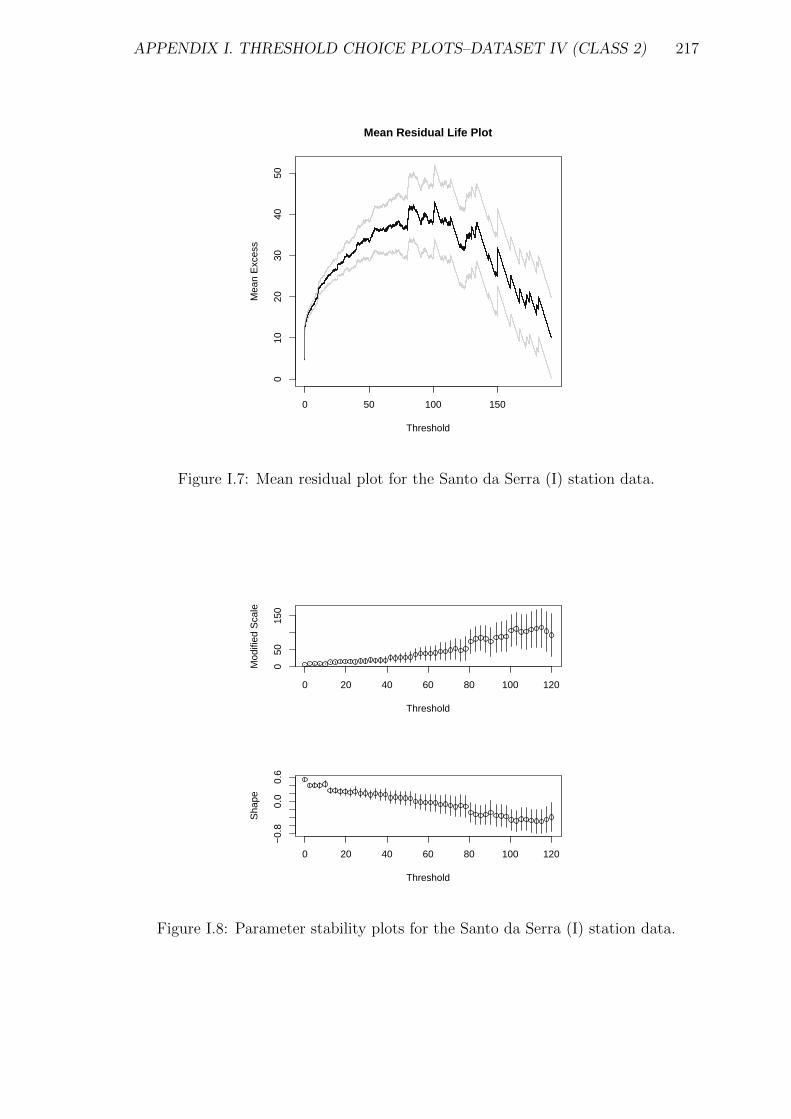
APPENDIX I. THRESHOLD CHOICE PLOTS–DATASET IV (CLASS 2) 217
0 50 100 150
010
2030
4050
Mean Residual Life Plot
Threshold
Mea
n E
xces
s
Figure I.7: Mean residual plot for the Santo da Serra (I) station data.
0 20 40 60 80 100 120
050
150
Threshold
Mod
ified
Sca
le
0 20 40 60 80 100 120
−0.
80.
00.
6
Threshold
Sha
pe
Figure I.8: Parameter stability plots for the Santo da Serra (I) station data.

218
0 20 40 60 80 100 120
020
4060
8010
0
Mean Residual Life Plot
Threshold
Mea
n E
xces
s
Figure I.9: Mean residual plot for the Porto Moniz (J) station data.
0 20 40 60 80
−30
00
200
Threshold
Mod
ified
Sca
le
0 20 40 60 80
−1
13
Threshold
Sha
pe
Figure I.10: Parameter stability plots for the Porto Moniz (J) station data.

APPENDIX I. THRESHOLD CHOICE PLOTS–DATASET IV (CLASS 2) 219
0 50 100 150
010
2030
40
Mean Residual Life Plot
Threshold
Mea
n E
xces
s
Figure I.11: Mean residual plot for the Curral das Freiras (K) station data.
0 20 40 60 80 100 120
5015
0
Threshold
Mod
ified
Sca
le
0 20 40 60 80 100 120
−0.
80.
0
Threshold
Sha
pe
Figure I.12: Parameter stability plots for the Curral das Freiras (K) station data.

220

Appendix J
Threshold choice plots – Dataset
IV (Class 3)
Mean residual and parameter stability plots for the
stations with altitude between 300 and 600 m
221
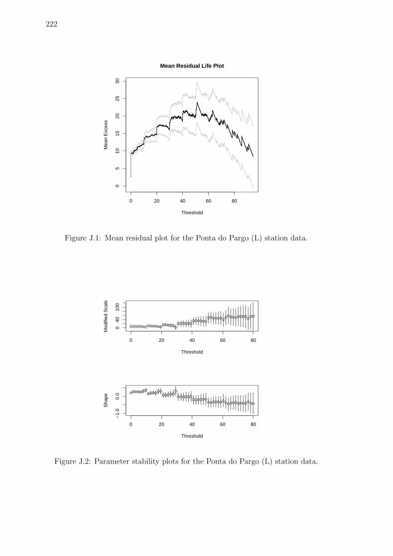
222
0 20 40 60 80
05
1015
2025
30
Mean Residual Life Plot
Threshold
Mea
n E
xces
s
Figure J.1: Mean residual plot for the Ponta do Pargo (L) station data.
0 20 40 60 80
040
100
Threshold
Mod
ified
Sca
le
0 20 40 60 80
−1.
00.
0
Threshold
Sha
pe
Figure J.2: Parameter stability plots for the Ponta do Pargo (L) station data.
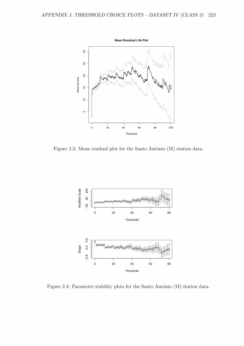
APPENDIX J. THRESHOLD CHOICE PLOTS – DATASET IV (CLASS 3) 223
0 20 40 60 80 100
510
1520
2530
Mean Residual Life Plot
Threshold
Mea
n E
xces
s
Figure J.3: Mean residual plot for the Santo Antonio (M) station data.
0 20 40 60 80
−20
4010
0
Threshold
Mod
ified
Sca
le
0 20 40 60 80
−0.
80.
00.
6
Threshold
Sha
pe
Figure J.4: Parameter stability plots for the Santo Antonio (M) station data.
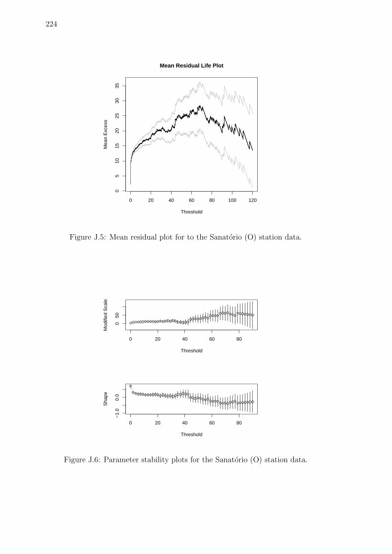
224
0 20 40 60 80 100 120
05
1015
2025
3035
Mean Residual Life Plot
Threshold
Mea
n E
xces
s
Figure J.5: Mean residual plot for to the Sanatorio (O) station data.
0 20 40 60 80
050
Threshold
Mod
ified
Sca
le
0 20 40 60 80
−1.
00.
0
Threshold
Sha
pe
Figure J.6: Parameter stability plots for the Sanatorio (O) station data.
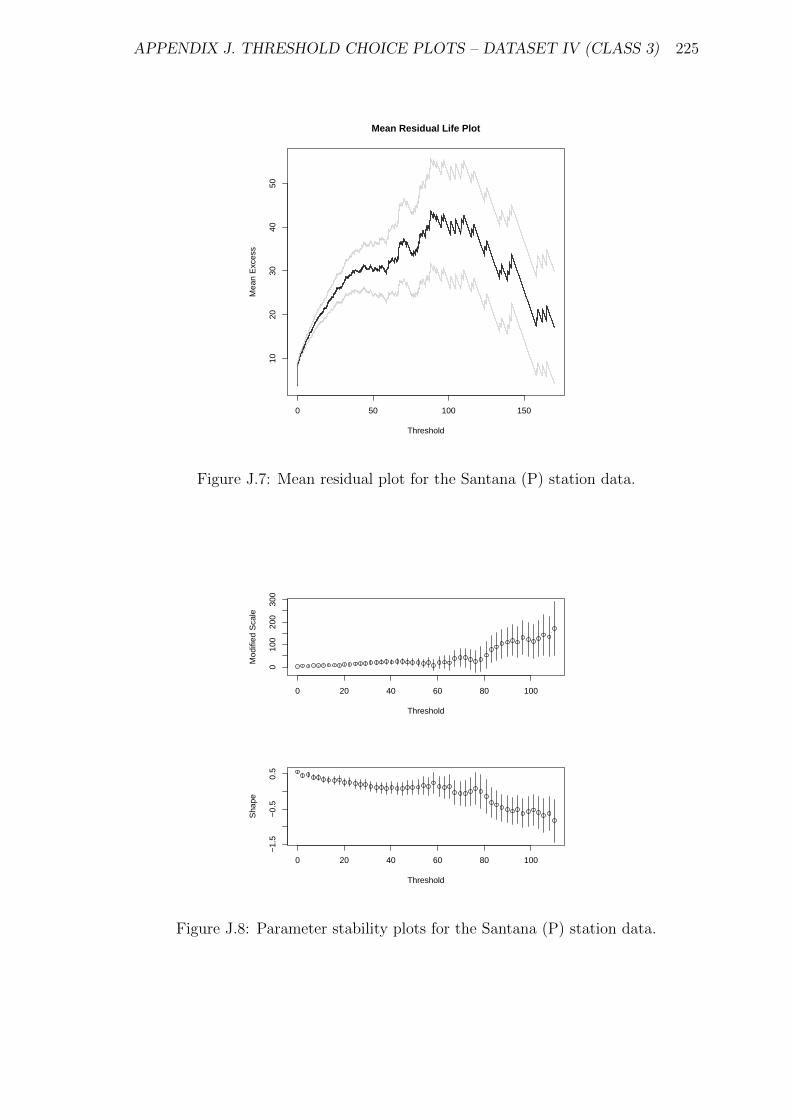
APPENDIX J. THRESHOLD CHOICE PLOTS – DATASET IV (CLASS 3) 225
0 50 100 150
1020
3040
50
Mean Residual Life Plot
Threshold
Mea
n E
xces
s
Figure J.7: Mean residual plot for the Santana (P) station data.
0 20 40 60 80 100
010
020
030
0
Threshold
Mod
ified
Sca
le
0 20 40 60 80 100
−1.
5−
0.5
0.5
Threshold
Sha
pe
Figure J.8: Parameter stability plots for the Santana (P) station data.
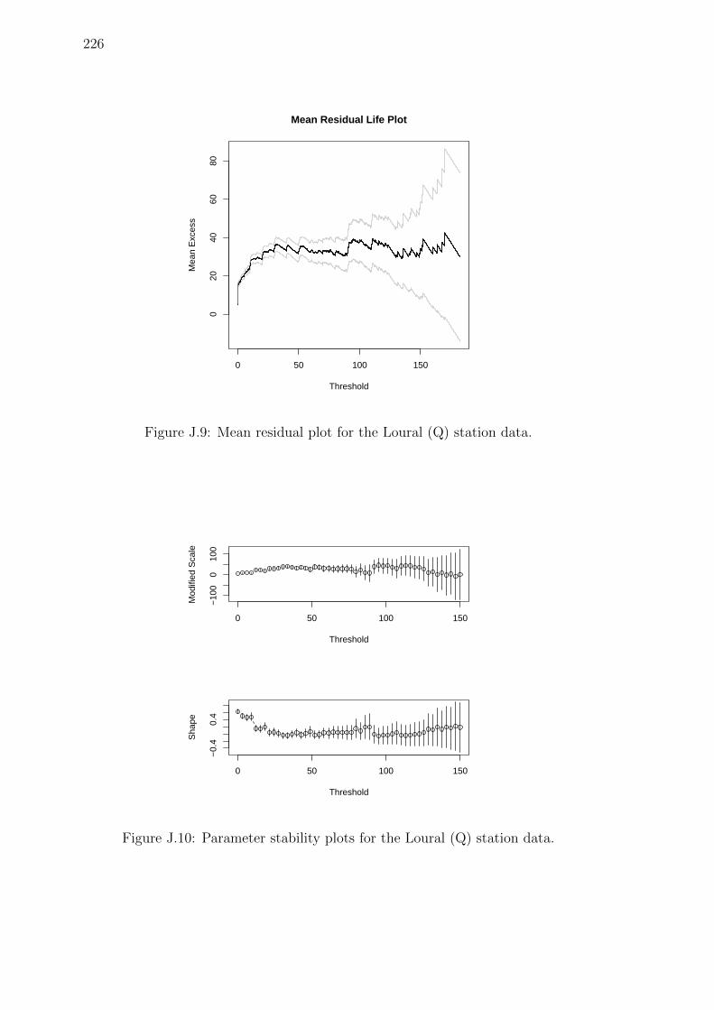
226
0 50 100 150
020
4060
80
Mean Residual Life Plot
Threshold
Mea
n E
xces
s
Figure J.9: Mean residual plot for the Loural (Q) station data.
0 50 100 150
−10
00
100
Threshold
Mod
ified
Sca
le
0 50 100 150
−0.
40.
4
Threshold
Sha
pe
Figure J.10: Parameter stability plots for the Loural (Q) station data.

Appendix K
Threshold choice plots – Dataset
IV (Class 4)
Mean residual and parameter stability plots for the
stations with altitude below 300 m
227
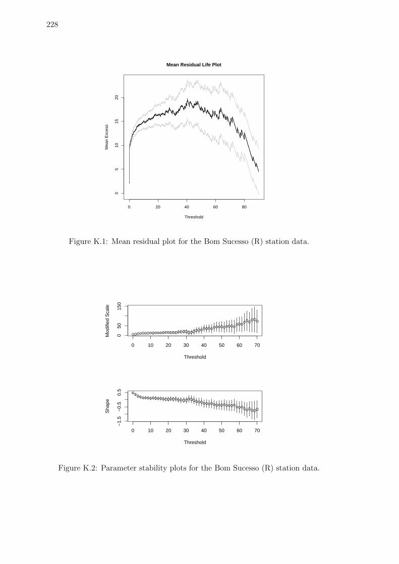
228
0 20 40 60 80
05
1015
20
Mean Residual Life Plot
Threshold
Mea
n E
xces
s
Figure K.1: Mean residual plot for the Bom Sucesso (R) station data.
0 10 20 30 40 50 60 70
050
150
Threshold
Mod
ified
Sca
le
0 10 20 30 40 50 60 70
−1.
5−
0.5
0.5
Threshold
Sha
pe
Figure K.2: Parameter stability plots for the Bom Sucesso (R) station data.
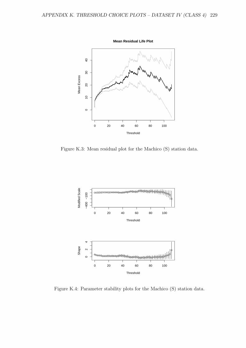
APPENDIX K. THRESHOLD CHOICE PLOTS – DATASET IV (CLASS 4) 229
0 20 40 60 80 100
010
2030
40
Mean Residual Life Plot
Threshold
Mea
n E
xces
s
Figure K.3: Mean residual plot for the Machico (S) station data.
0 20 40 60 80 100
−40
0−
100
Threshold
Mod
ified
Sca
le
0 20 40 60 80 100
02
4
Threshold
Sha
pe
Figure K.4: Parameter stability plots for the Machico (S) station data.
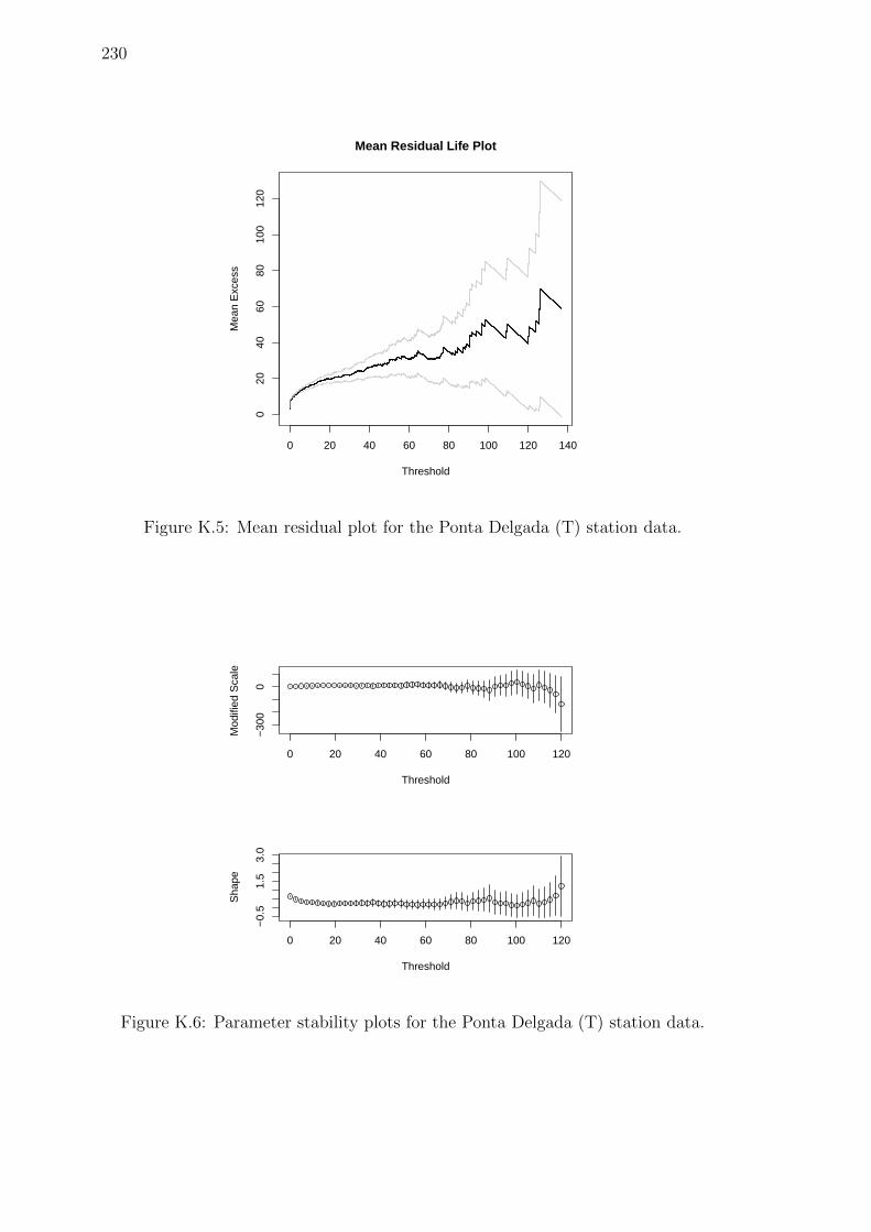
230
0 20 40 60 80 100 120 140
020
4060
8010
012
0
Mean Residual Life Plot
Threshold
Mea
n E
xces
s
Figure K.5: Mean residual plot for the Ponta Delgada (T) station data.
0 20 40 60 80 100 120
−30
00
Threshold
Mod
ified
Sca
le
0 20 40 60 80 100 120
−0.
51.
53.
0
Threshold
Sha
pe
Figure K.6: Parameter stability plots for the Ponta Delgada (T) station data.
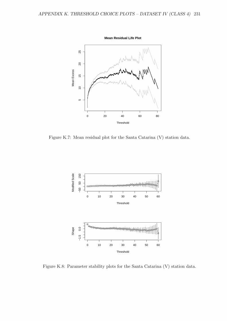
APPENDIX K. THRESHOLD CHOICE PLOTS – DATASET IV (CLASS 4) 231
0 20 40 60 80
510
1520
25
Mean Residual Life Plot
Threshold
Mea
n E
xces
s
Figure K.7: Mean residual plot for the Santa Catarina (V) station data.
0 10 20 30 40 50 60
−50
5015
0
Threshold
Mod
ified
Sca
le
0 10 20 30 40 50 60
−1.
50.
0
Threshold
Sha
pe
Figure K.8: Parameter stability plots for the Santa Catarina (V) station data.

232
0 20 40 60 80
05
1015
2025
30
Mean Residual Life Plot
Threshold
Mea
n E
xces
s
Figure K.9: Mean residual plot for the Canical (W) station data.
0 10 20 30 40
040
100
Threshold
Mod
ified
Sca
le
0 10 20 30 40
−1.
00.
0
Threshold
Sha
pe
Figure K.10: Parameter stability plots for the Canical (W) station data.
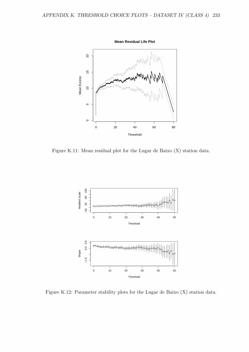
APPENDIX K. THRESHOLD CHOICE PLOTS – DATASET IV (CLASS 4) 233
0 20 40 60 80
05
1015
20
Mean Residual Life Plot
Threshold
Mea
n E
xces
s
Figure K.11: Mean residual plot for the Lugar de Baixo (X) station data.
0 10 20 30 40 50
−20
2060
100
Threshold
Mod
ified
Sca
le
0 10 20 30 40 50
−1.
00.
00.
5
Threshold
Sha
pe
Figure K.12: Parameter stability plots for the Lugar de Baixo (X) station data.
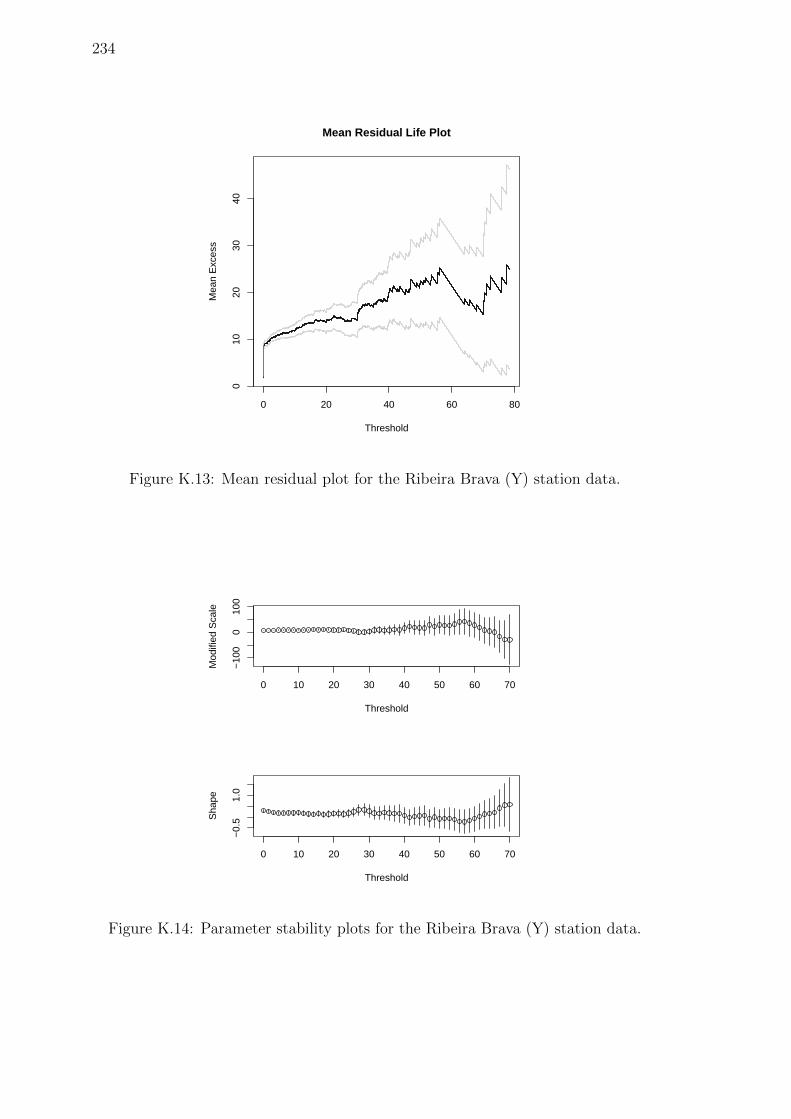
234
0 20 40 60 80
010
2030
40
Mean Residual Life Plot
Threshold
Mea
n E
xces
s
Figure K.13: Mean residual plot for the Ribeira Brava (Y) station data.
0 10 20 30 40 50 60 70
−10
00
100
Threshold
Mod
ified
Sca
le
0 10 20 30 40 50 60 70
−0.
51.
0
Threshold
Sha
pe
Figure K.14: Parameter stability plots for the Ribeira Brava (Y) station data.
Appendix L
Exceedances percentage by month
– Dataset IV
235

236
Table L.1: Exceedances percentage by month for u1.
Station J F M A M J J A S O N D
Areeiro (A) 23 14 10 3 3 1 0 0 3 10 17 15
Bica da Cana (B) 22 13 12 5 2 2 0 0 2 13 15 14
Poiso (C) 18 18 9 2 3 3 0 0 3 7 22 13
Montado do Pereiro (D) 18 17 12 4 4 1 0 0 3 9 18 13
Encumeada (E) 26 15 11 4 2 2 0 0 3 8 13 16
Ribeiro Frio (F) 18 17 9 5 3 1 0 1 5 10 17 15
Queimadas (G) 20 12 9 5 2 1 1 1 5 15 16 12
Camacha (H) 21 16 10 6 3 2 1 0 3 5 20 15
Santo da Serra (I) 21 12 10 5 2 2 1 1 3 13 17 13
Porto Moniz (J) 18 14 8 2 2 2 1 2 5 14 22 11
Curral das Freiras (K) 21 9 16 6 2 2 0 0 4 9 18 14
Ponta do Pargo (L) 26 9 16 4 1 1 0 0 3 7 25 8
Santo Antonio (M) 19 17 12 5 1 1 0 0 2 10 16 16
Canhas (N) 19 11 11 5 2 3 1 2 2 20 11 16
Sanatorio (O) 16 15 10 5 1 1 0 1 3 8 23 17
Santana (P) 19 11 6 4 3 1 1 2 5 16 16 15
Loural (Q) 18 19 11 6 2 2 0 0 2 11 18 12
Bom Sucesso (R) 15 18 6 8 1 2 0 0 5 12 21 13
Machico (S) 12 19 11 5 1 2 1 1 3 14 19 12
Ponta Delgada (T) 20 14 10 5 2 1 0 2 2 19 17 8
Funchal (U) 18 14 8 6 1 2 0 0 3 12 19 16
Santa Catarina (V) 22 17 7 5 2 1 0 0 4 12 16 12
Canical (W) 16 15 12 6 2 2 1 0 3 15 17 14
Lugar de Baixo (X) 23 13 9 3 2 1 0 0 3 15 16 15
Ribeira Brava (Y) 24 12 11 3 1 3 0 0 4 14 14 16
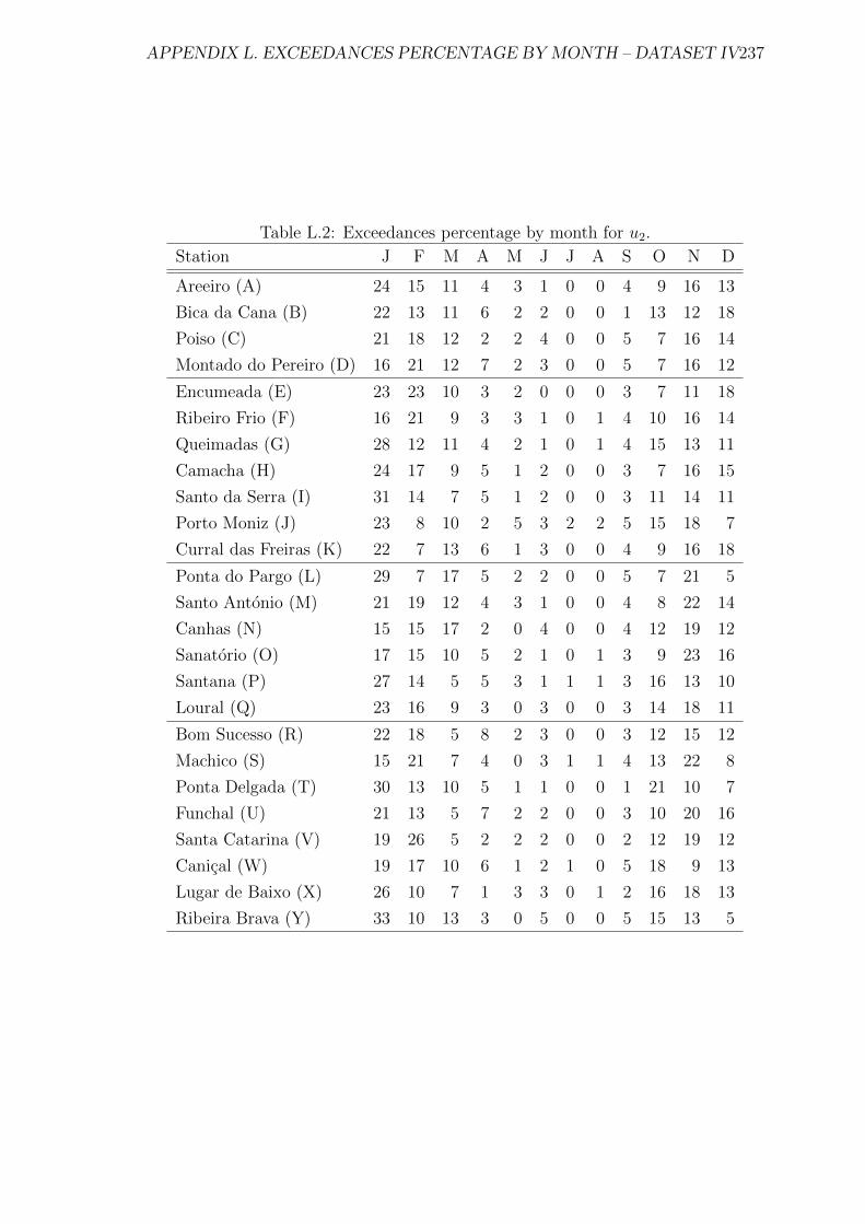
APPENDIX L. EXCEEDANCES PERCENTAGE BY MONTH – DATASET IV237
Table L.2: Exceedances percentage by month for u2.
Station J F M A M J J A S O N D
Areeiro (A) 24 15 11 4 3 1 0 0 4 9 16 13
Bica da Cana (B) 22 13 11 6 2 2 0 0 1 13 12 18
Poiso (C) 21 18 12 2 2 4 0 0 5 7 16 14
Montado do Pereiro (D) 16 21 12 7 2 3 0 0 5 7 16 12
Encumeada (E) 23 23 10 3 2 0 0 0 3 7 11 18
Ribeiro Frio (F) 16 21 9 3 3 1 0 1 4 10 16 14
Queimadas (G) 28 12 11 4 2 1 0 1 4 15 13 11
Camacha (H) 24 17 9 5 1 2 0 0 3 7 16 15
Santo da Serra (I) 31 14 7 5 1 2 0 0 3 11 14 11
Porto Moniz (J) 23 8 10 2 5 3 2 2 5 15 18 7
Curral das Freiras (K) 22 7 13 6 1 3 0 0 4 9 16 18
Ponta do Pargo (L) 29 7 17 5 2 2 0 0 5 7 21 5
Santo Antonio (M) 21 19 12 4 3 1 0 0 4 8 22 14
Canhas (N) 15 15 17 2 0 4 0 0 4 12 19 12
Sanatorio (O) 17 15 10 5 2 1 0 1 3 9 23 16
Santana (P) 27 14 5 5 3 1 1 1 3 16 13 10
Loural (Q) 23 16 9 3 0 3 0 0 3 14 18 11
Bom Sucesso (R) 22 18 5 8 2 3 0 0 3 12 15 12
Machico (S) 15 21 7 4 0 3 1 1 4 13 22 8
Ponta Delgada (T) 30 13 10 5 1 1 0 0 1 21 10 7
Funchal (U) 21 13 5 7 2 2 0 0 3 10 20 16
Santa Catarina (V) 19 26 5 2 2 2 0 0 2 12 19 12
Canical (W) 19 17 10 6 1 2 1 0 5 18 9 13
Lugar de Baixo (X) 26 10 7 1 3 3 0 1 2 16 18 13
Ribeira Brava (Y) 33 10 13 3 0 5 0 0 5 15 13 5

238
Appendix M
Code of the functions
implemented in R
239

240
Code of the functions applied in Section 5.2
Code for the normalized Hasofer and Wang test statistic, W ∗n(k), defined by (4.15):
esttesteHWNA < −function(x, k){n < −length(x)
q < −(1/k)
ordx < −sort(x)
j < −n− ki < −j + 1
threshold < −ordx[j]
u < −ordx[i : n]
z < −u− thresholdv < −z∧2soma1 < −sum(z)
soma2 < −sum(v)
prod1 < −q ∗ soma1
prod2 < −q ∗ soma2
quad < −(prod1)∧2
w < −q ∗ (quad/(prod2− quad))
return(w)}
arauxHW1 < −function(m){vectorf < −dataset$variablek < −mfvalorHW < −esttesteHWNA(vectorf, k)
vobser < −sqrt(k/4) ∗ (k ∗ fvalorHW − 1)
return(vobser)}
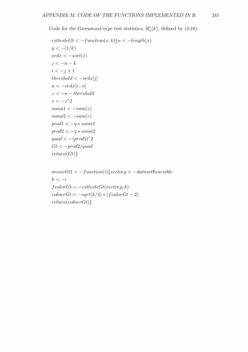
APPENDIX M. CODE OF THE FUNCTIONS IMPLEMENTED IN R 241
Code for the Greenwood type test statistics, R∗n(k), defined by (4.16):
esttesteGt < −function(x, k){n < −length(x)
q < −(1/k)
ordx < −sort(x)
j < −n− ki < −j + 1
threshold < −ordx[j]
u < −ordx[i : n]
z < −u− thresholdv < −z∧2soma1 < −sum(z)
soma2 < −sum(v)
prod1 < −q ∗ soma1
prod2 < −q ∗ soma2
quad < −(prod1)∧2
Gt < −prod2/quad
return(Gt)}
arauxGt1 < −function(i){vectorg < −dataset$variablek < −ifvalorGt < −esttesteGt(vectorg, k)
vobserGt < −sqrt(k/4) ∗ (fvalorGt− 2)
return(vobserGt)}

242
Code of the functions applied in Section 5.3
Code for the parameters βi (4.42), with i ∈ {1, 2, 3} from the copula function:
betaic < −function(u, v, w){valorbeta < −1/((1/2) ∗ (1 + ((1/u) + (1/v)− (1/w))))
return(valorbeta)}
Code for the copula function C defined by (4.31):
copexperiencia < −function(a, b, c, d, e, f){valorcopula < −(a∧(1− d)) ∗ (b∧(1− e)) ∗ (c∧(1− f)) ∗min((a∧d), (b∧e), (c∧f))
return(valorcopula)}
Code for the function used to compute probability pq = P (Eq) defined by (4.43):
funcaop < −function(a, b, c, d, e, f){parcela1 < −(1− a− b− c)parcela2 < −copexperiencia(a, b, c, d, e, f)
parcela3 < −copexperiencia(a, b, 1, d, e, f)
parcela4 < −copexperiencia(a, 1, c, d, e, f)
parcela5 < −copexperiencia(1, b, c, d, e, f)
valorp < −parcela1− parcela2 + parcela3 + parcela4 + parcela5
return(valorp)}