Deliverable 6-C: Software and Algorithms to Support ... · . 3 Colling, T., & Schlaff, G. (2012)

“Focusing on education, research, and development of technology to sense and understand natural and

manmade environments."

“Meeting our transportation needs through innovative research, distinctive educational programs, technology transfer, and workforce development.”

Prepared By: Michigan Tech Research Institute Michigan Tech Center for Technology & Training Michigan Technological University

Michigan Technological University

Characterization of Unpaved Road

Condition Through the Use of Remote Sensing

Deliverable 6-C: Software and Algorithms to Support Unpaved Road Assessment by Remote

Sensing

Submitted version of: October 31, 2012

Authors: Chris Roussi, [email protected]

Tim Colling, PhD., P.E., [email protected] David Dean, [email protected]

Colin Brooks, [email protected] Gary Schlaff, [email protected] Luke Peterson, [email protected]

Melanie Kueber Watkins, P.E., [email protected] Richard Dobson, [email protected]

Justin Carter, [email protected]

www.mtri.org/unpaved

Deliverable 6-C: Software and Algorithms to Support Unpaved Road Assessment by Remote Sensing

2

Acknowledgements ....................................................................................................................................... 4

Purpose of this Document ............................................................................................................................. 4

Motivation ..................................................................................................................................................... 4

Part 1: Demonstration of DSS Software and Functions ................................................................................ 5

Identify Unpaved Road Network ............................................................................................................ 5

URCI Distress Type, Quantity, Severity Data and Density Calculation ................................................. 6

URCI Distress Deduct Value Calculation ............................................................................................... 8

Distress Index Calculation .................................................................................................................... 11

Use of URCI Data in the DSS ............................................................................................................... 12

DSS Continued Development ............................................................................................................... 17

Part 2: Software and Algorithms Developed and Applied for Analysis of Unpaved Road Condition Imagery. ...................................................................................................................................................... 17

Software Development .......................................................................................................................... 17

Software Architecture Philosophy ........................................................................................................ 17

Software Toolbox .................................................................................................................................. 18

The Bash Shell ........................................................................................................................................ 18

The Python Interpreter .......................................................................................................................... 18

The Processing Scheme .......................................................................................................................... 19

Third-Party Tools ................................................................................................................................... 19

Name ....................................................................................................................................................... 19

Source ..................................................................................................................................................... 19

Description ............................................................................................................................................. 19

Processing Functional Flow .................................................................................................................. 20

Image Quality Check ............................................................................................................................. 20

Preprocessing ........................................................................................................................................ 21

Scale-invariant Feature Transform ........................................................................................................ 21

Bundler .................................................................................................................................................. 21

Patch-based Multi-view Stereo ............................................................................................................. 21

Depth Map ............................................................................................................................................. 21

Distress Extraction ................................................................................................................................ 22

Distress Characterization ...................................................................................................................... 22


3

Analysis ................................................................................................................................................. 22

Feature Translation ................................................................................................................................ 22

Example Case ........................................................................................................................................ 23

Summary ..................................................................................................................................................... 26

Part 3: Unpaved Road Identification and Classification. ............................................................................ 26

Concluding Comments ........................................................................................................................... 33

Appendix A: Deduct Value Curves ............................................................................................................ 35


4

Acknowledgements

This work is supported by the Commercial Remote Sensing and Spatial Information (CRS&SI) program of the Research and Innovative Technology Administration (RITA), U.S. Department of Transportation (USDOT), under Cooperative Agreement RITARS-11-H-MTU1, with additional support provided by the South East Michigan Council of Governments (SEMCOG), the Michigan Transportation Asset Management Council (TAMC), the Road Commission for Oakland County (RCOC), and the Michigan Tech Transportation Institute (MTTI). The views, opinions, findings, and conclusions reflected in this paper are the responsibility of the authors only and do not represent the official policy or position of the USDOT, RITA, or any state or other entity. Additional information regarding this project can be found at www.mtri.org/unpaved.

Purpose of this Document

This report is focused on summarizing the software acquired or developed during this project including the Decision Support System (DSS), image analysis components, and the road surface type data being used as an input for mission planning. It includes an update on progress on integrating distress data into the commercially available RoadSoft GIS tool being used as a demonstration of DSS capabilities for unpaved road management for this project. Also included is a detailed description of the software tools and algorithms being used to process remote sensing data of road condition into usable information. Finally, an update on progress in developing and applying a robust unpaved roads mapping algorithm using readily available color-infrared aerial photography is included.

Motivation

One of the main goals outlined for the Characterization of Unpaved Roads by Remote Sensing project was to show that data collected through remote sensing can be effectively used in a decision support system for managing unpaved roads. Management of unpaved roads has historically been challenged by the lack of a method or system that provides decision support and enables cost-effective data collection. Systems providing decision support or basic distress identification for unpaved roads have been developed, but data collection costs and quality have limited their effectiveness and adoption by unpaved road managers. It is the goal of this project to overcome these limitations by providing an example of how data can be collected cost-effectively from remote sensing systems using a standard road assessment and inventory technique1

and how this data can be integrated into a DSS. The DSS makes use of a variety of data, including asset inventory data, condition (distress) data, and project history data to allow users to more quickly make informed asset management decisions, and to see the impacts of these decisions on the long term health of their road network.

1Department of the Army. (1995). Unsurfaced Road Maintenance Management Technical Manual No. 5-626.

Washington DC: United States Department of The Army.

http://www.mtri.org/unpaved�


5

Part 1: Demonstration of DSS Software and Functions The DSS provides an interface for storing, organizing and analyzing large quantities of data that assists users in determining a course of action. The DSS that was used for this project is the commercially available product called RoadSoft which uses a geographic information system (GIS) interface to spatially locate and display data related to transportation assets. More information on the DSS can be found at the RoadSoft web site (www.roadsoft.org) as was first reviewed for this project in Deliverable 6-B. The DSS received data from two specific remote sensing and analysis processes. The road type Trimble eCognition-based process produces the unpaved road inventory information that the DSS used to identify the unpaved road network (see the second half of Deliverable 6-A, A Demonstration Mission Planning System for use in Remote Sensing the Phenomena of Unpaved Road Conditions2 and the third section of this report. The remote sensing platform system (RSPS) (sensor plus platforms) produces road distress data and inventory feature data that the DSS uses to determine asset conditions. A detailed explanation of how the DSS, road type mapping, and RSPS systems work together and the data cycle associated with them was first presented in project Deliverable 6-B: A Demonstration Decision Support System for Managing Unpaved Roads in RoadSoft3

Identify Unpaved Road Network

.

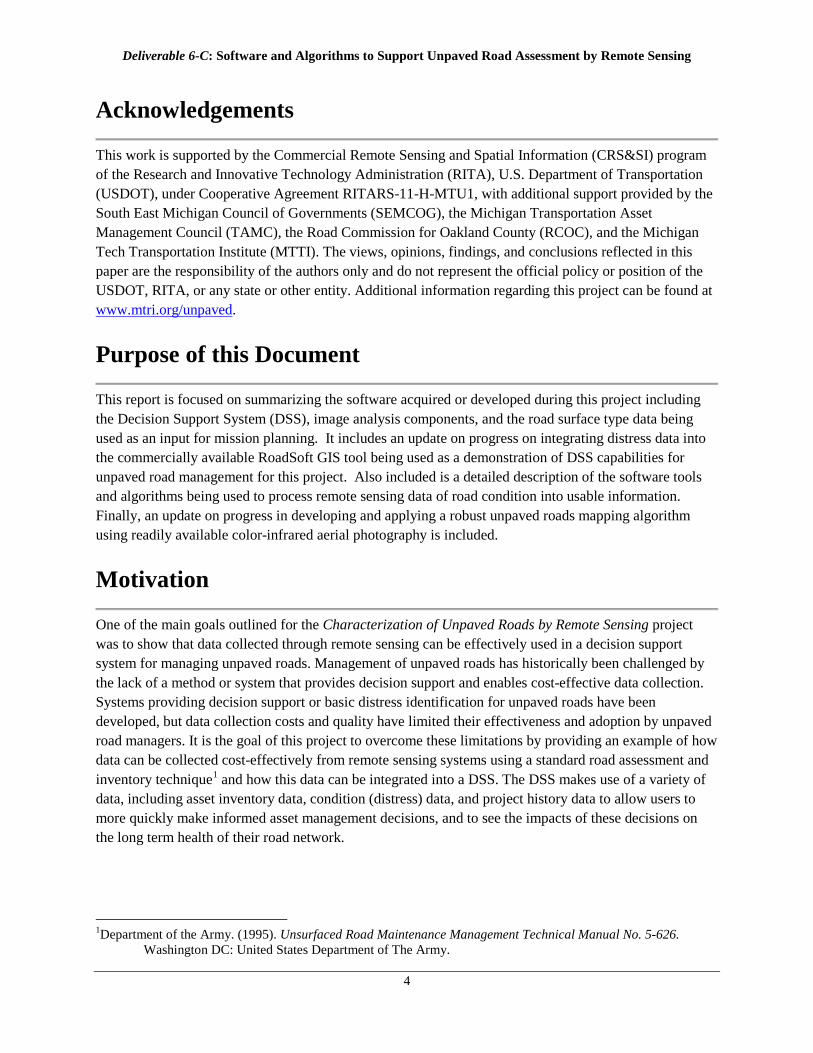
The DSS uses unpaved road inventory data from the aerial imagery analysis to update its existing pavement surface inventory from historical data if any exists. Road segments in the DSS that are identified as being unpaved in the aerial imagery analysis, but that do not have a pavement type assigned in the DSS, are set as “pavement type=gravel”. Road segments in the DSS that had an existing pavement surface type will only be assigned “pavement type=gravel” when most current surface type information in the DSS is older than the aerial image date used for the analysis. This logic ensures that the newest data will be used to determine pavement types from a combination of historical and new data. Figure 1 provides an example of an updated road inventory in the DSS.

2 Roussi, C., C. Brooks, A. Vander Woude. (2012). Deliverable 6-A: A Demonstration Mission Planning System for

use in Remote Sensing the Phenomena of Unpaved Road Conditions. 16 pgs. Available at http://geodjango.mtri.org/unpaved/media/doc/deliverable_Del6A_MissionPlanningSystemReport.pdf

3 Colling, T., & Schlaff, G. (2012). Deliverable 6-B: A Demonstration of Unpaved Road Condition Through the Use of Remote Sensing. 31 pgs.

http://www.roadsoft.org/�

http://geodjango.mtri.org/unpaved/media/doc/deliverable_Del6A_MissionPlanningSystemReport.pdf�


6

Figure 1: Example of an updated unpaved road inventory in the DSS (RoadSoft).

Unpaved roads shown as orange dashes. URCI Distress Type, Quantity, Severity Data and Density Calculation Raw data collected by the remote sensing platform system (RSPS) during field collects to acquire distress data require post processing to convert the raw data to URCI categories prior to export to the DSS. Information on quantity and severity of the five distresses defined by the URCI (Unsurfaced Road Condition Index) method4

are collected by the RSPS and are available for import into the DSS.

These distresses include: • loss of road cross section, • improper drainage (where possible) • potholes • ruts • corrugations (washboarding) • loose aggregate berms

4 Brooks, C., T. Colling, M. Kueber, C. Roussi, K.A. Endsley. (2011). Deliverable 2-A: State of the Practice of

Unpaved Road Condition Assessment. 50 pgs. Available at http://geodjango.mtri.org/unpaved/media/doc/deliverable_Del2-A_State_of_the_Practice_for_Unpaved_Roads_MichiganTech.pdf

http://geodjango.mtri.org/unpaved/media/doc/deliverable_Del2-A_State_of_the_Practice_for_Unpaved_Roads_MichiganTech.pdf�

http://geodjango.mtri.org/unpaved/media/doc/deliverable_Del2-A_State_of_the_Practice_for_Unpaved_Roads_MichiganTech.pdf�


7

The URCI method also has a distress measure for dust but that distress was determined to be infeasible to be collected by remote sensing. The DSS can accept manually collected distress data for dust measurements, or any of the other URCI distresses. The URCI method classifies distress severity into three severity bins of low, medium, or high severity. The criteria to sort specific distress into these bins are defined by the URCI method itself where there is a quantitative measurement associated with the severity level. Several distresses, such as improper cross section and loss of drainage do not contain a quantitative measure for determining their severity bin. Quantitative measures for each of these more qualitative distresses are proposed in 6-B5

(Colling & Schlaff, 2012).

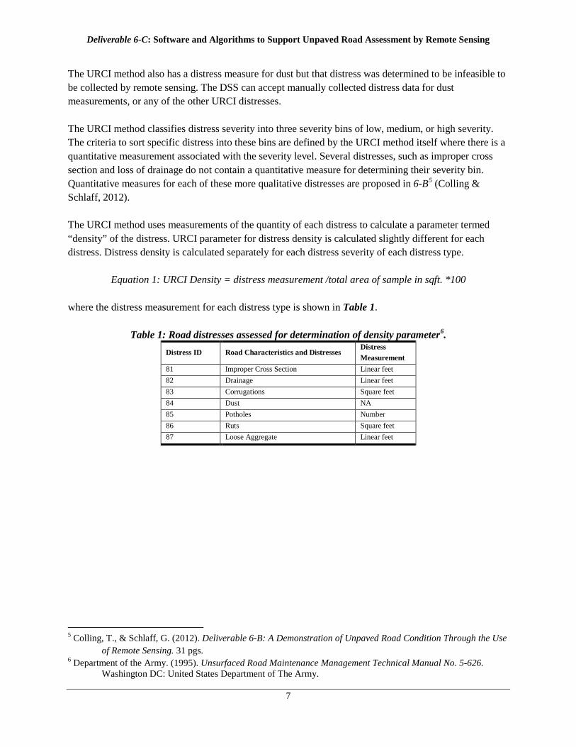
The URCI method uses measurements of the quantity of each distress to calculate a parameter termed “density” of the distress. URCI parameter for distress density is calculated slightly different for each distress. Distress density is calculated separately for each distress severity of each distress type.

Equation 1: URCI Density = distress measurement /total area of sample in sqft. *100

where the distress measurement for each distress type is shown in Table 1.

Table 1: Road distresses assessed for determination of density parameter6

Distress ID

. Road Characteristics and Distresses

Distress Measurement

81 Improper Cross Section Linear feet 82 Drainage Linear feet 83 Corrugations Square feet 84 Dust NA 85 Potholes Number 86 Ruts Square feet 87 Loose Aggregate Linear feet

5 Colling, T., & Schlaff, G. (2012). Deliverable 6-B: A Demonstration of Unpaved Road Condition Through the Use

of Remote Sensing. 31 pgs. 6 Department of the Army. (1995). Unsurfaced Road Maintenance Management Technical Manual No. 5-626.



8

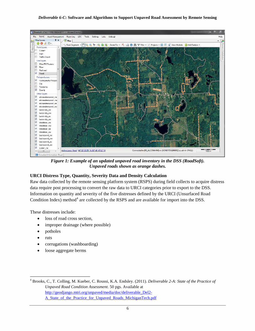
The DSS has been developed to store and display URCI data relating to a segment of road, as shown in Figure 2. The quantity and extent of each URCI distress can either be received from the RSPS or user-entered from manual collection activities.

URCI Distress Deduct Value Calculation The URCI method uses unique plots of distress density and severity to calculate URCI deduct point values for each distress. Distresses higher in severity and density accumulated more deduct values7

.

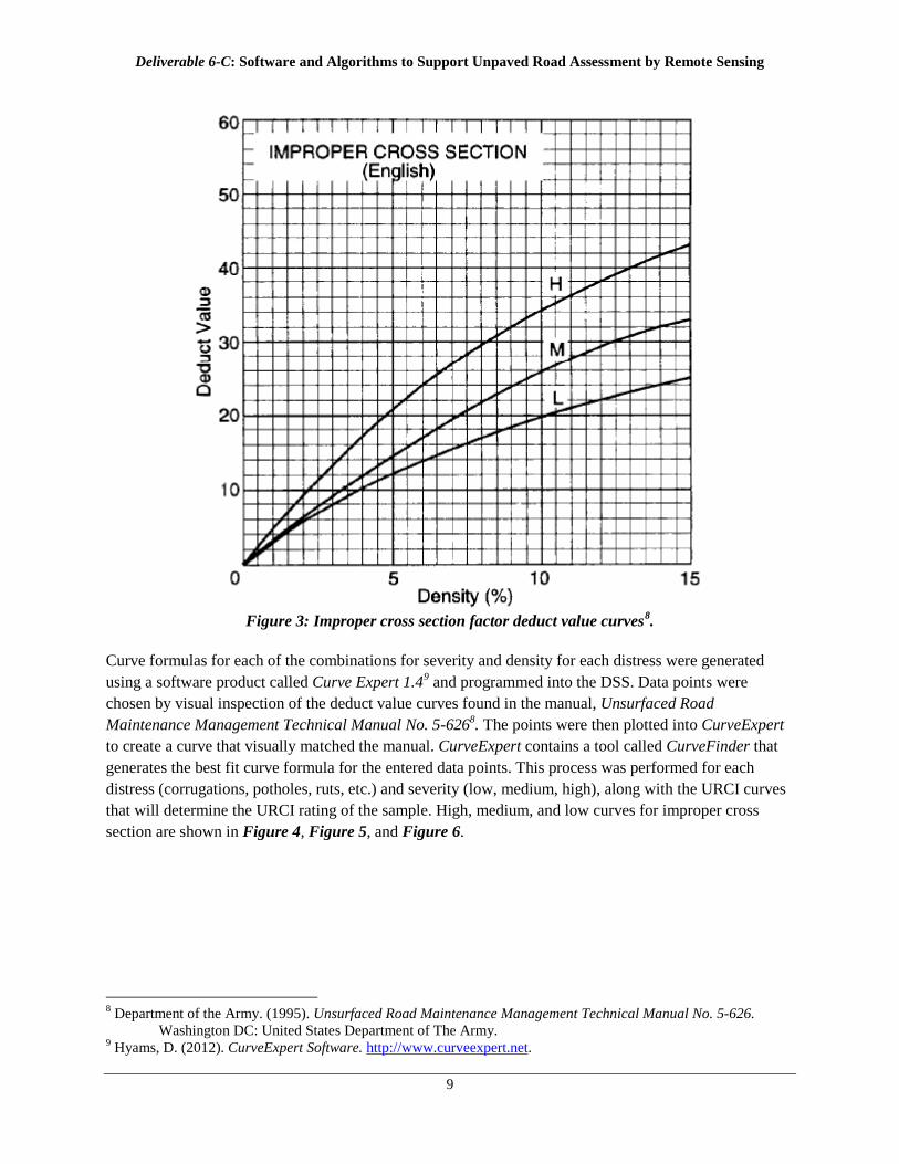
An example of a deduct value curve for the improper cross section factor is shown in Figure 3 below. The deduct curves for the remainder of the distresses are shown in Appendix A.

7 Department of the Army. (1995). Unsurfaced Road Maintenance Management Technical Manual No. 5-626.


Figure 2: DSS data form showing distress quantity for each distress severity and type.


9

Figure 3: Improper cross section factor deduct value curves8

.

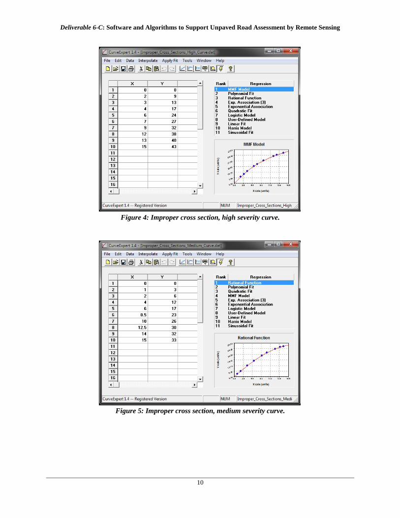
Curve formulas for each of the combinations for severity and density for each distress were generated using a software product called Curve Expert 1.49

Figure 4

and programmed into the DSS. Data points were chosen by visual inspection of the deduct value curves found in the manual, Unsurfaced Road Maintenance Management Technical Manual No. 5-6268. The points were then plotted into CurveExpert to create a curve that visually matched the manual. CurveExpert contains a tool called CurveFinder that generates the best fit curve formula for the entered data points. This process was performed for each distress (corrugations, potholes, ruts, etc.) and severity (low, medium, high), along with the URCI curves that will determine the URCI rating of the sample. High, medium, and low curves for improper cross section are shown in , Figure 5, and Figure 6.


Washington DC: United States Department of The Army. 9 Hyams, D. (2012). CurveExpert Software. http://www.curveexpert.net.

http://www.curveexpert.net/�


10

Figure 4: Improper cross section, high severity curve.

Figure 5: Improper cross section, medium severity curve.


11

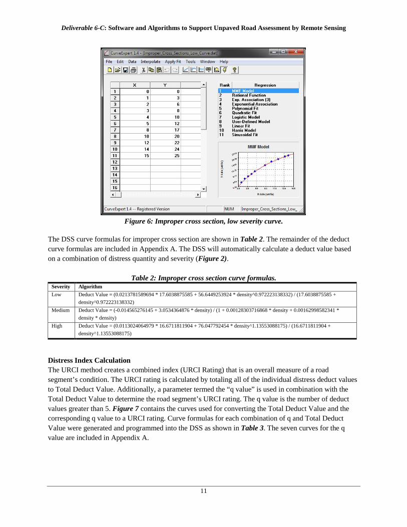
Figure 6: Improper cross section, low severity curve.

The DSS curve formulas for improper cross section are shown in Table 2. The remainder of the deduct curve formulas are included in Appendix A. The DSS will automatically calculate a deduct value based on a combination of distress quantity and severity (Figure 2).

Table 2: Improper cross section curve formulas. Severity Algorithm Low Deduct Value = (0.0213781589694 * 17.6038875585 + 56.6449253924 * density^0.972223138332) / (17.6038875585 +

density^0.972223138332) Medium Deduct Value = (-0.014565276145 + 3.0534364876 * density) / (1 + 0.00128303716868 * density + 0.00162998582341 *

density * density) High Deduct Value = (0.0113024064979 * 16.6711811904 + 76.047792454 * density^1.13553088175) / (16.6711811904 +

density^1.13553088175)

Distress Index Calculation The URCI method creates a combined index (URCI Rating) that is an overall measure of a road segment’s condition. The URCI rating is calculated by totaling all of the individual distress deduct values to Total Deduct Value. Additionally, a parameter termed the “q value” is used in combination with the Total Deduct Value to determine the road segment’s URCI rating. The q value is the number of deduct values greater than 5. Figure 7 contains the curves used for converting the Total Deduct Value and the corresponding q value to a URCI rating. Curve formulas for each combination of q and Total Deduct Value were generated and programmed into the DSS as shown in Table 3. The seven curves for the q value are included in Appendix A.


12

Figure 7: Total deduct value10

.

Table 3: Total deduct value curve formulas. Severity Algorithm q = 1 urci = 100 - totalDeductValue q = 2 urci = 99.442556802 + -0.702281190257 * totalDeductValue + -0.000908764111217 * totalDeductValue^2 +

0.00000945743530741 * totalDeductValue^3 q = 3 urci = 106.628343108 + -0.834213315131 * totalDeductValue + 0.00138080609451 * totalDeductValue^2 q = 4 urci = 105.042340814 + -0.582137674653 * totalDeductValue + -0.00131723014292 * totalDeductValue^2 +

0.00000826614167894 * totalDeductValue^3 q = 5 urci = 106.118811703 + -0.543444824815 * totalDeductValue + -0.00110649065181 * totalDeductValue^2 +



0.00000868306923091 * totalDeductValue^3

Information from the RSPS can be augmented with other distress or inventory data from manual field inspections as users deem necessary. Data for the dust distress measurements would be required to be manually collected and entered since it is infeasible to reliably measure this distress with remote sensing to the extent necessary to make the data usable, at least within the context of this project.

Use of URCI Data in the DSS A user interface was developed for the DSS to allow inspection of each of the road sample segments and the respective distress data. Figure 8 shows an example of the user interface in the DSS showing recently collected URCI distress data for a given sample segment.




13

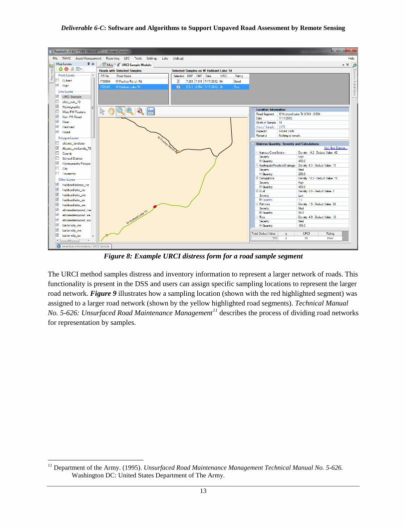
Figure 8: Example URCI distress form for a road sample segment

The URCI method samples distress and inventory information to represent a larger network of roads. This functionality is present in the DSS and users can assign specific sampling locations to represent the larger road network. Figure 9 illustrates how a sampling location (shown with the red highlighted segment) was assigned to a larger road network (shown by the yellow highlighted road segments). Technical Manual No. 5-626: Unsurfaced Road Maintenance Management11

describes the process of dividing road networks for representation by samples.




14

Figure 9: Assigning road sampling locations to a network of representative roads in the DSS.

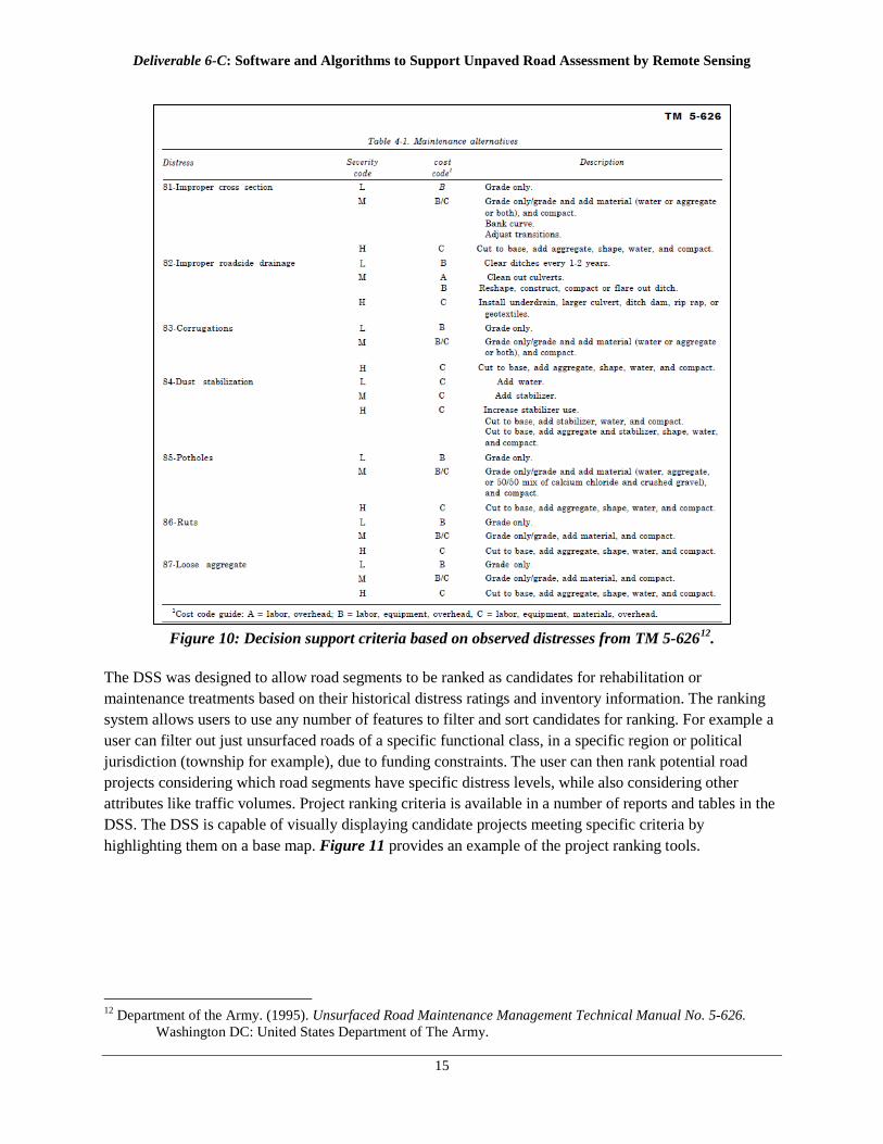
The URCI method provides a set of decision support criteria that guides a road manager to a specific course of action based on an observed road distress or condition. An example of decision support criteria is shown in Figure 10. These criteria were designed specifically for U.S. military facilities to standardize decision making given the resources and criticality of the transportation systems they were intended for. However, they may not necessarily be the best practice or provide suitable guidance for public road managers with large unpaved road systems. The DSS developed for use in this project allows individual road agencies to customize the applicable decision-making criteria based on their individual agency goals, resources and practice.


15

Figure 10: Decision support criteria based on observed distresses from TM 5-62612

.

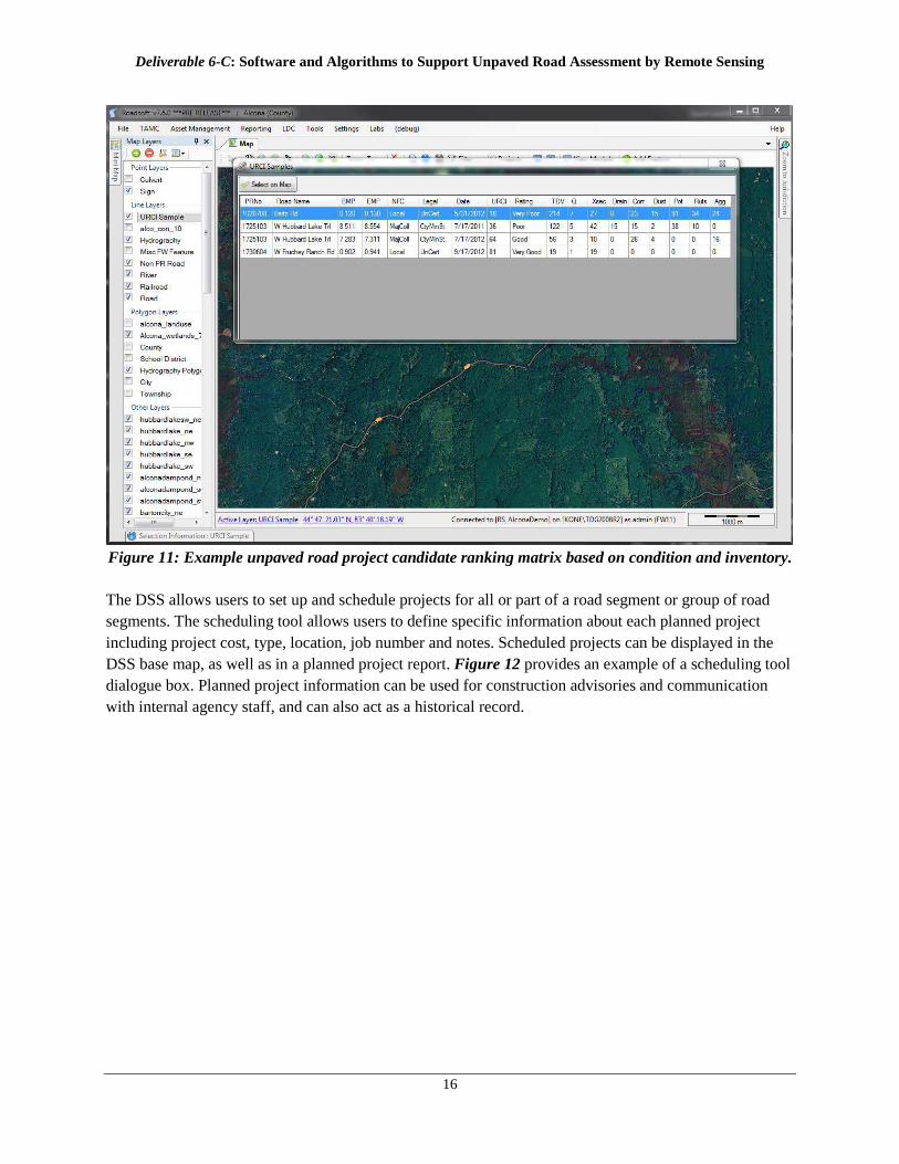
The DSS was designed to allow road segments to be ranked as candidates for rehabilitation or maintenance treatments based on their historical distress ratings and inventory information. The ranking system allows users to use any number of features to filter and sort candidates for ranking. For example a user can filter out just unsurfaced roads of a specific functional class, in a specific region or political jurisdiction (township for example), due to funding constraints. The user can then rank potential road projects considering which road segments have specific distress levels, while also considering other attributes like traffic volumes. Project ranking criteria is available in a number of reports and tables in the DSS. The DSS is capable of visually displaying candidate projects meeting specific criteria by highlighting them on a base map. Figure 11 provides an example of the project ranking tools.




16

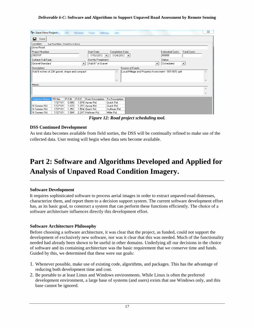
Figure 11: Example unpaved road project candidate ranking matrix based on condition and inventory. The DSS allows users to set up and schedule projects for all or part of a road segment or group of road segments. The scheduling tool allows users to define specific information about each planned project including project cost, type, location, job number and notes. Scheduled projects can be displayed in the DSS base map, as well as in a planned project report. Figure 12 provides an example of a scheduling tool dialogue box. Planned project information can be used for construction advisories and communication with internal agency staff, and can also act as a historical record.


17

Figure 12: Road project scheduling tool.

DSS Continued Development As test data becomes available from field sorties, the DSS will be continually refined to make use of the collected data. User testing will begin when data sets become available.

Part 2: Software and Algorithms Developed and Applied for Analysis of Unpaved Road Condition Imagery.

Software Development It requires sophisticated software to process aerial images in order to extract unpaved-road distresses, characterize them, and report them to a decision support system. The current software development effort has, as its basic goal, to construct a system that can perform these functions efficiently. The choice of a software architecture influences directly this development effort.

Software Architecture Philosophy Before choosing a software architecture, it was clear that the project, as funded, could not support the development of exclusively new software, nor was it clear that this was needed. Much of the functionality needed had already been shown to be useful in other domains. Underlying all our decisions in the choice of software and its containing architecture was the basic requirement that we conserve time and funds. Guided by this, we determined that these were our goals: 1. Whenever possible, make use of existing code, algorithms, and packages. This has the advantage of

reducing both development time and cost. 2. Be portable to at least Linux and Windows environments. While Linux is often the preferred

development environment, a large base of systems (and users) exists that use Windows only, and this base cannot be ignored.


18

3. Modularity. This allows various functional blocks to be “swapped out” as needed, to try different algorithms, without impacting the overall software system (again, reducing development time and costs).

4. Whenever possible, use tools that are license-free, or do not incur excessive recurring costs. This would exclude, for example, an implementation in MatLab.

5. Use the most up-to-date techniques possible. This ensures that the system does not become functionally obsolete before it can be distributed, and makes the best use of current knowledge in signal analysis and processing.

Based on these goals, we elected to use certain tools, packages, and computer languages, as described below. Because the packages to be incorporated in the system were written in a variety of languages, we were driven to use a generic environment, with custom-written interfaces between the existing software packages.

Software Toolbox Rather than a system developed in a single environment (e.g. a tool written using ENVI only), we have pulled together a variety of environments and tools (a “toolbox”, with many drawers). This was done by choosing a most basic control structure, which is based on a command-line shell (“bash”) and packages interpreted by that shell. This forms the “glue” which binds together the various components of the system. It does not contribute to the functions needed to meet the system requirements, but exists solely to interconnect components.

The Bash Shell The program that starts processes, interprets commands, and handles user inputs is called a “command shell”, or just “shell”. The one we use is named “bash”. It was released in 1989 as part of the Unix operating system, and as a replacement for the Bourne Shell (“sh”). It has since been deployed across Linux, MacOS, Windows, Android, and even Novell Netware. This command interpreter forms the basis for the control of our software system. The bash syntax is sufficiently complex that it can be considered a computer programming language in its own right. However, it was intended primarily for job-control (at which it excels), and something else is needed for inter-process communication and numerical manipulation.

The Python Interpreter Like bash, Python is an interpreted language, and is often used as a scripting language. Like bash, it was released in 1989. Unlike bash, it is a general-purpose, high-level, object-oriented programming language, with a large number of supporting packages that perform functions ranging from scientific analysis (sciPy, numpy, etc.) to interprocess communications. Python runs on Linux, Windows, MacOS, and has been ported to Java and the .NET virtual machines. And there is precedent for using Python in environmental processing; ESRI recommends using Python to develop ArcGIS scripts13

.

Much of the code that we have developed is either written in, controlled by, or accesses native libraries of, Python. Although Python is invoked by bash, in many cases it performs many of the control functions of bash, in a sense replacing it once it starts running.

13 http://webhelp.esri.com/arcgisdesktop/9.2/index.cfm?TopicName=About_getting_started_with_ writing_geoprocessing_scripts

http://webhelp.esri.com/arcgisdesktop/9.2/index.cfm?TopicName=About_getting_started_with_writing_geoprocessing_scripts�

http://webhelp.esri.com/arcgisdesktop/9.2/index.cfm?TopicName=About_getting_started_with_writing_geoprocessing_scripts�


19

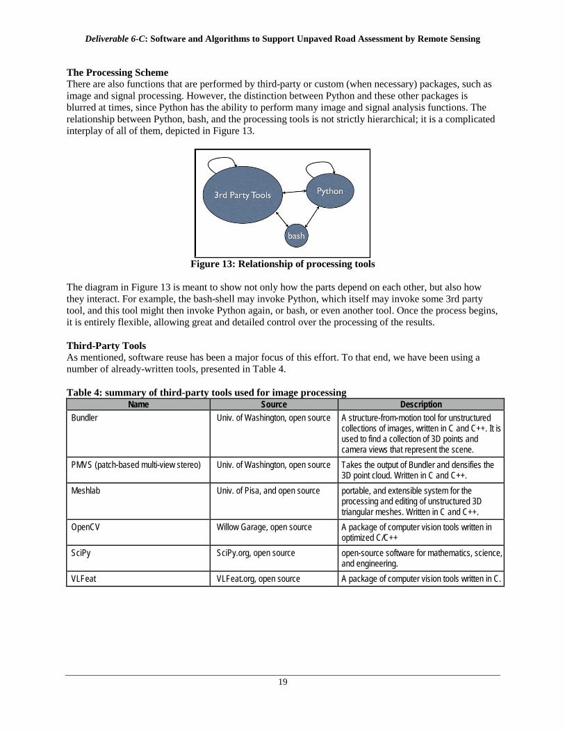
The Processing Scheme There are also functions that are performed by third-party or custom (when necessary) packages, such as image and signal processing. However, the distinction between Python and these other packages is blurred at times, since Python has the ability to perform many image and signal analysis functions. The relationship between Python, bash, and the processing tools is not strictly hierarchical; it is a complicated interplay of all of them, depicted in Figure 13.

Figure 13: Relationship of processing tools

The diagram in Figure 13 is meant to show not only how the parts depend on each other, but also how they interact. For example, the bash-shell may invoke Python, which itself may invoke some 3rd party tool, and this tool might then invoke Python again, or bash, or even another tool. Once the process begins, it is entirely flexible, allowing great and detailed control over the processing of the results. Third-Party Tools As mentioned, software reuse has been a major focus of this effort. To that end, we have been using a number of already-written tools, presented in Table 4. Table 4: summary of third-party tools used for image processing

Name Source Description Bundler Univ. of Washington, open source A structure-from-motion tool for unstructured

collections of images, written in C and C++. It is used to find a collection of 3D points and camera views that represent the scene.

PMVS (patch-based multi-view stereo) Univ. of Washington, open source Takes the output of Bundler and densifies the 3D point cloud. Written in C and C++.

Meshlab Univ. of Pisa, and open source portable, and extensible system for the processing and editing of unstructured 3D triangular meshes. Written in C and C++.

OpenCV Willow Garage, open source A package of computer vision tools written in optimized C/C++

SciPy SciPy.org, open source open-source software for mathematics, science, and engineering.

VLFeat VLFeat.org, open source A package of computer vision tools written in C.


20

Most of these tools are generally not useful in a stand-alone fashion; we have had to write drivers and “glue-code” in order to make use of these tools. All are free to use, and may be redistributed freely, with certain provisions.14,15

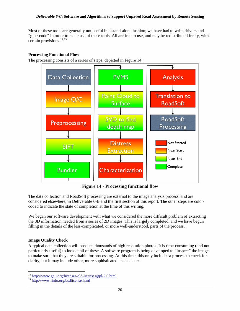
Processing Functional Flow The processing consists of a series of steps, depicted in Figure 14.

Figure 14 - Processing functional flow

The data collection and RoadSoft processing are external to the image analysis process, and are considered elsewhere, in Deliverable 6-B and the first section of this report. The other steps are color-coded to indicate the state of completion at the time of this writing. We began our software development with what we considered the more difficult problem of extracting the 3D information needed from a series of 2D images. This is largely completed, and we have begun filling in the details of the less-complicated, or more well-understood, parts of the process.

Image Quality Check A typical data collection will produce thousands of high resolution photos. It is time-consuming (and not particularly useful) to look at all of these. A software program is being developed to “inspect” the images to make sure that they are suitable for processing. At this time, this only includes a process to check for clarity, but it may include other, more sophisticated checks later. 14 http://www.gnu.org/licenses/old-licenses/gpl-2.0.html 15 http://www.linfo.org/bsdlicense.html

http://www.gnu.org/licenses/old-licenses/gpl-2.0.html�

http://www.linfo.org/bsdlicense.html�


21

Preprocessing This step prepares an image for processing by the downstream software. It may include resampling the image (if it is too high a resolution, for example, we may want to make it smaller to improve throughput), sharpening the image, or other simple steps to make the image more likely to be useful to subsequent programs.

Scale-invariant Feature Transform Objects in an image exhibit “interesting points” (e.g. corners) that can be extracted as features of that object. For reliable recognition, those features (called “keypoints”) should be detected even if the scale of the image changes (the object is larger or smaller), there is noise in the image (like other objects nearby), or the illumination changes between images. Also, the relative positions between the features should not change from one image to another. Being able to identify the same feature in two different images, possibly taken from different locations, is important to the process of 3D reconstruction to follow. An algorithm to perform this function, first published in 1999, is available. Called SIFT16

Bundler

, it finds so-called “keypoints” of objects in an image, and stores them in a database of such features. Then, in another image, “keypoints” are found, and the Euclidean distance between those features and the stored features is found. If the features are in substantial agreement in terms of scale, location, and orientation, then they are listed as “good” matches, and “bad” matches are discarded. If there are 3 or more such features that match, they are subjected to a more detailed verification, and the probability of the presence of an object is computed (based on the accuracy of the match, and the number of the probably false matches). These matches are passed to the Bundler process.

This takes a set of images, and the image features and matches (from SIFT), and produces a 3D reconstruction of camera positions and a sparse scene geometry as output. The scene is reconstructed incrementally, a few images at-a-time, based on the sparse-bundle adjustment package of Lourakis and Argyros17

Patch-based Multi-view Stereo

. In other words, it produces sparse point-clouds in 3D representing objects in the image. These point-clouds can be useful, but for our purposes, we need a denser representation (more points in the cloud). For this, we need the next algorithm.

This package, provided by Yasutaka Furukawa18

Depth Map

, takes a set of images and camera parameters, and reconstructs the 3D structure of an object or a scene. It ignores non-rigid objects, and outputs a set of points that represent the rigid scene (not a mesh model) containing both the 3D coordinates and the surface normal at each point.

The process of generating a depth map from the dense point cloud takes multiple steps, outlined below: 1. Form a surface from the points. This can be done quickly using a Poisson reconstruction19, or more

slowly (but more accurately) by a ball-pivoting operation20

16 D. G. Lowe, “Distinctive image features from scale-invariant keypoints”, International Journal of Computer

Vision, 60, 2, (2004), pp 91-110

.

17 http://www.ics.forth.gr/~lourakis/sba/ 18 Y. Furukawa, J. Ponce, “Accurate, Dense, and Robust Multi-View Stereopsis”, IEEE Trans. on Pattern Analysis

and Machine Intelligence, 2010, vol. 32, no. 8, pp. 1362-1376 19 M. Kazhdan, M. Bolitho, H. Hoppe, “Poisson Surface Reconstruction”, Proc. of Eurographics Symposium on

Geometry Processing, 2006.

http://www.ics.forth.gr/~lourakis/sba/�


22

2. Smooth the surface, to remove reconstruction outliers. An example algorithm is Taubin smoothing21

3. Find the transformation that maps the plane of the road into the X-Y plane. When this is done, the Z-axis is the height field. This can be most conveniently performed using Singular Value Decomposition

.

22

(SVD).

Once we have the depth map, a variety of operations may be performed to evaluate the nature of the surface, including finding distresses.

Distress Extraction The first problem becomes locating those areas of the surface to characterize. The distresses that we are finding include: 1. Potholes. These are detected, and their locations and sizes determined, using a modified circular

Hough-Transform23

2. Ruts. These are detected using a Gabor filter.

24

3. Corrugations. These, too, are found using a Gabor filter. formulation.

4. Crown. This feature is found by taking a cut through the surface orthogonal to the road direction in the image.

5. Loose aggregate. Detected as berms on the road surface not associated with ruts. The various quantities are measured, and passed on to the characterization stage.

Distress Characterization In this stage, the various requirements on ranking damages are applied. For example, potholes are sorted into bins based on their diameter, depth, etc. The number of potholes in each bin is what is used in analysis and reporting.

Analysis The abstracted distress information can then be summarized, statistics found, and reported for use in Decision Support Tools such as RoadSoft.

Feature Translation The RoadSoft program is expecting the data to be presented at its interface in some form, in a tabular format with fields that match those described in Appendix A: "XML Field Descriptions in the DSS from the eCognition System" as described on page 26 in Deliverable 6-B. A program will be written, based on the interface description, which will translate the numbers we measure into numbers acceptable to RoadSoft. In some cases, this may be as simple a unit conversion. In other cases, it may be somewhat more difficult; we are in the process of creating the interface control document (ICD) which will define the process of translation for us.

20 F. Bernardi, J. Mittleman, H. Rushmeier, C. Silva, G. Taubin, “The Ball-Pivoting Algorithm for Surface

Reconstruction”, IEEE Trans. on Visualization and Computer Graphics, 1999, vol. 5, pp. 349-359. 21G. Taubin. “A signal processing approach to fair surface design”. Proceedings of ACM SIGGRAPH 95, pages

351–358, 1995. 22 G. Golub, W. Kahan,"Calculating the singular values and pseudo-inverse of a matrix". Journal of the Society for

Industrial and Applied Mathematics: Series B, Numerical Analysis, 1965, 2 (2): 205–224 23 M. Rizon, H. Yazid, P. Saad, A. Shakaff, A. R. Saad, M. Sugisaka, S. Yaacob, M. R. Mamat, and M. Karthigayan,

“Object detection using circular hough transform”, American Journal of Applied Sciences 2 (12), 2005. 24 S. Grigorescu, N. Petkov, P. Kruizinga, “Comparison of Texture Features Based on Gabor Filters”, IEEE Trans.

on Image Processing, vol. 11, no. 10, 2002.


23

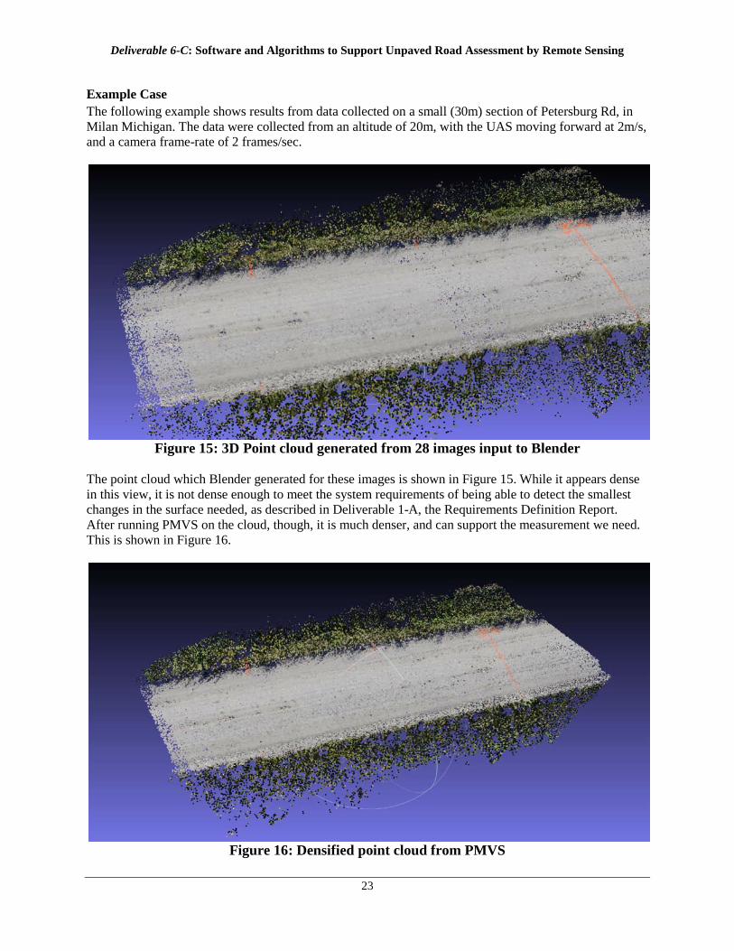
Example Case The following example shows results from data collected on a small (30m) section of Petersburg Rd, in Milan Michigan. The data were collected from an altitude of 20m, with the UAS moving forward at 2m/s, and a camera frame-rate of 2 frames/sec.

Figure 15: 3D Point cloud generated from 28 images input to Blender

The point cloud which Blender generated for these images is shown in Figure 15. While it appears dense in this view, it is not dense enough to meet the system requirements of being able to detect the smallest changes in the surface needed, as described in Deliverable 1-A, the Requirements Definition Report. After running PMVS on the cloud, though, it is much denser, and can support the measurement we need. This is shown in Figure 16.

Figure 16: Densified point cloud from PMVS


24

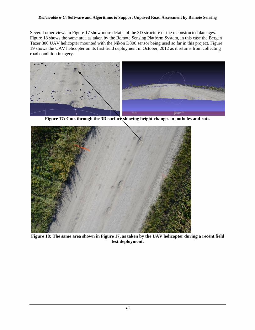
Several other views in Figure 17 show more details of the 3D structure of the reconstructed damages. Figure 18 shows the same area as taken by the Remote Sensing Platform System, in this case the Bergen Tazer 800 UAV helicopter mounted with the Nikon D800 sensor being used so far in this project. Figure 19 shows the UAV helicopter on its first field deployment in October, 2012 as it returns from collecting road condition imagery.

Figure 17: Cuts through the 3D surface showing height changes in potholes and ruts.

Figure 18: The same area shown in Figure 17, as taken by the UAV helicopter during a recent field

test deployment.


25

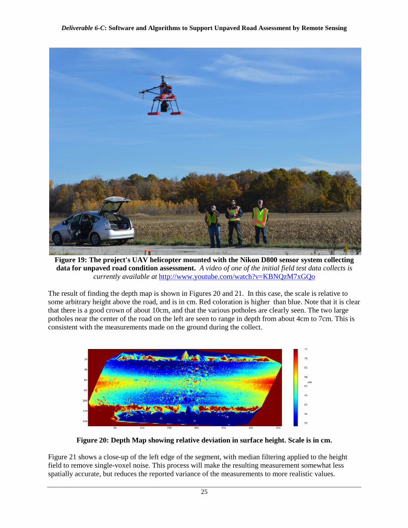
Figure 19: The project's UAV helicopter mounted with the Nikon D800 sensor system collecting data for unpaved road condition assessment. A video of one of the initial field test data collects is

currently available at http://www.youtube.com/watch?v=KBNQzM7xGQo The result of finding the depth map is shown in Figures 20 and 21. In this case, the scale is relative to some arbitrary height above the road, and is in cm. Red coloration is higher than blue. Note that it is clear that there is a good crown of about 10cm, and that the various potholes are clearly seen. The two large potholes near the center of the road on the left are seen to range in depth from about 4cm to 7cm. This is consistent with the measurements made on the ground during the collect.

Figure 20: Depth Map showing relative deviation in surface height. Scale is in cm.

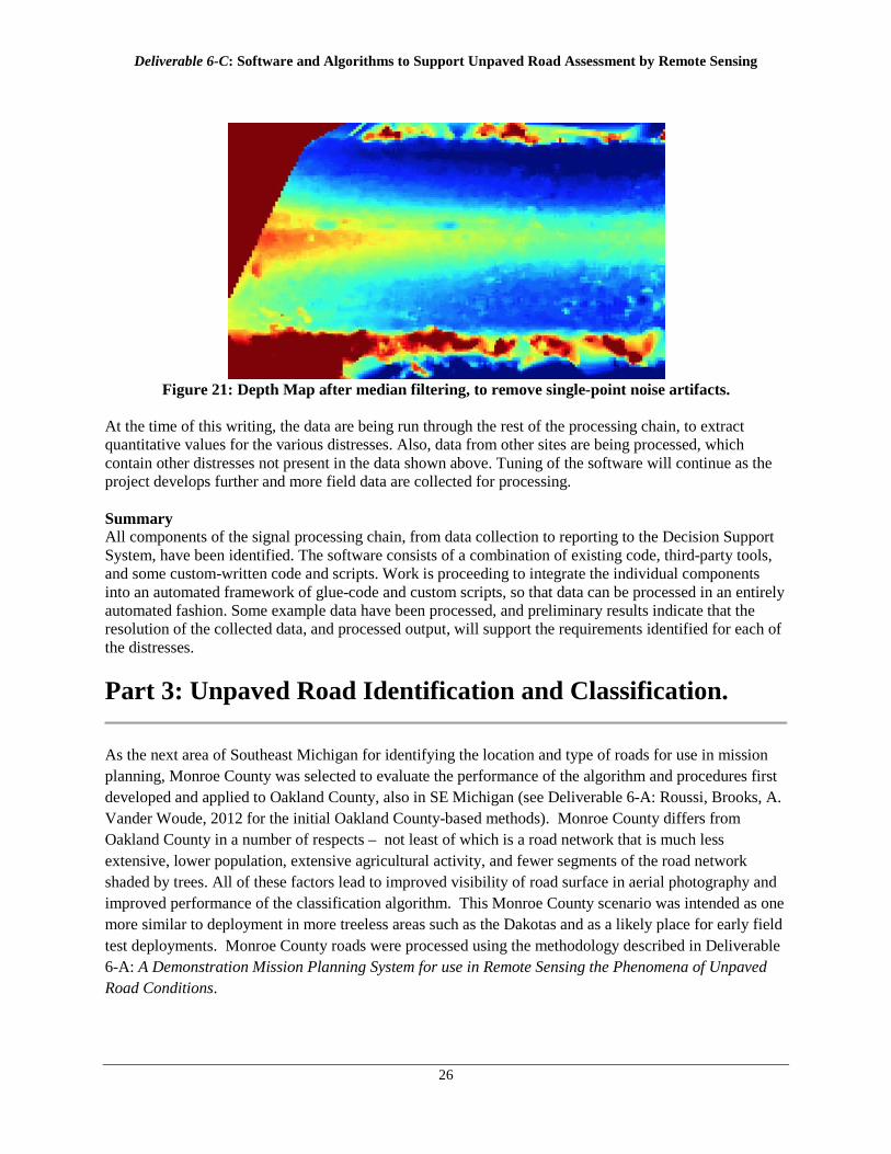
Figure 21 shows a close-up of the left edge of the segment, with median filtering applied to the height field to remove single-voxel noise. This process will make the resulting measurement somewhat less spatially accurate, but reduces the reported variance of the measurements to more realistic values.

http://www.youtube.com/watch?v=KBNQzM7xGQo�


26

Figure 21: Depth Map after median filtering, to remove single-point noise artifacts.

At the time of this writing, the data are being run through the rest of the processing chain, to extract quantitative values for the various distresses. Also, data from other sites are being processed, which contain other distresses not present in the data shown above. Tuning of the software will continue as the project develops further and more field data are collected for processing. Summary All components of the signal processing chain, from data collection to reporting to the Decision Support System, have been identified. The software consists of a combination of existing code, third-party tools, and some custom-written code and scripts. Work is proceeding to integrate the individual components into an automated framework of glue-code and custom scripts, so that data can be processed in an entirely automated fashion. Some example data have been processed, and preliminary results indicate that the resolution of the collected data, and processed output, will support the requirements identified for each of the distresses.

Part 3: Unpaved Road Identification and Classification.

As the next area of Southeast Michigan for identifying the location and type of roads for use in mission planning, Monroe County was selected to evaluate the performance of the algorithm and procedures first developed and applied to Oakland County, also in SE Michigan (see Deliverable 6-A: Roussi, Brooks, A. Vander Woude, 2012 for the initial Oakland County-based methods). Monroe County differs from Oakland County in a number of respects – not least of which is a road network that is much less extensive, lower population, extensive agricultural activity, and fewer segments of the road network shaded by trees. All of these factors lead to improved visibility of road surface in aerial photography and improved performance of the classification algorithm. This Monroe County scenario was intended as one more similar to deployment in more treeless areas such as the Dakotas and as a likely place for early field test deployments. Monroe County roads were processed using the methodology described in Deliverable 6-A: A Demonstration Mission Planning System for use in Remote Sensing the Phenomena of Unpaved Road Conditions.


27

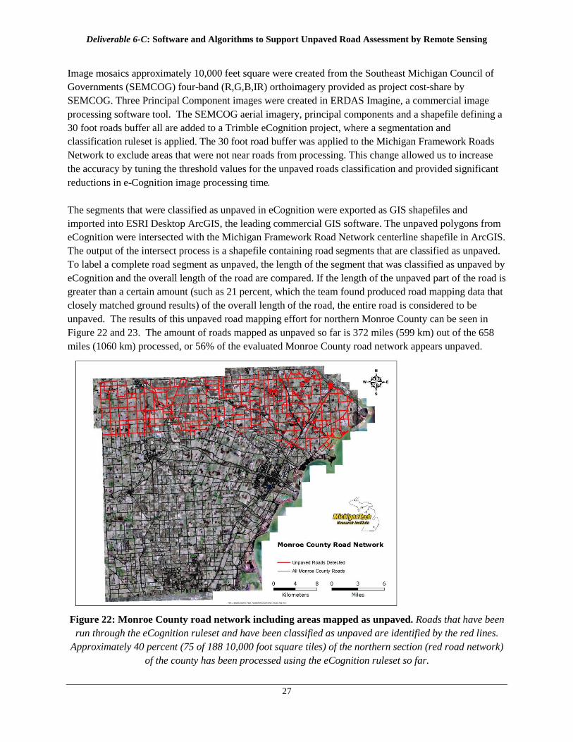
Image mosaics approximately 10,000 feet square were created from the Southeast Michigan Council of Governments (SEMCOG) four-band (R,G,B,IR) orthoimagery provided as project cost-share by SEMCOG. Three Principal Component images were created in ERDAS Imagine, a commercial image processing software tool. The SEMCOG aerial imagery, principal components and a shapefile defining a 30 foot roads buffer all are added to a Trimble eCognition project, where a segmentation and classification ruleset is applied. The 30 foot road buffer was applied to the Michigan Framework Roads Network to exclude areas that were not near roads from processing. This change allowed us to increase the accuracy by tuning the threshold values for the unpaved roads classification and provided significant reductions in e-Cognition image processing time. The segments that were classified as unpaved in eCognition were exported as GIS shapefiles and imported into ESRI Desktop ArcGIS, the leading commercial GIS software. The unpaved polygons from eCognition were intersected with the Michigan Framework Road Network centerline shapefile in ArcGIS. The output of the intersect process is a shapefile containing road segments that are classified as unpaved. To label a complete road segment as unpaved, the length of the segment that was classified as unpaved by eCognition and the overall length of the road are compared. If the length of the unpaved part of the road is greater than a certain amount (such as 21 percent, which the team found produced road mapping data that closely matched ground results) of the overall length of the road, the entire road is considered to be unpaved. The results of this unpaved road mapping effort for northern Monroe County can be seen in Figure 22 and 23. The amount of roads mapped as unpaved so far is 372 miles (599 km) out of the 658 miles (1060 km) processed, or 56% of the evaluated Monroe County road network appears unpaved.

Figure 22: Monroe County road network including areas mapped as unpaved. Roads that have been

run through the eCognition ruleset and have been classified as unpaved are identified by the red lines. Approximately 40 percent (75 of 188 10,000 foot square tiles) of the northern section (red road network)

of the county has been processed using the eCognition ruleset so far.


28

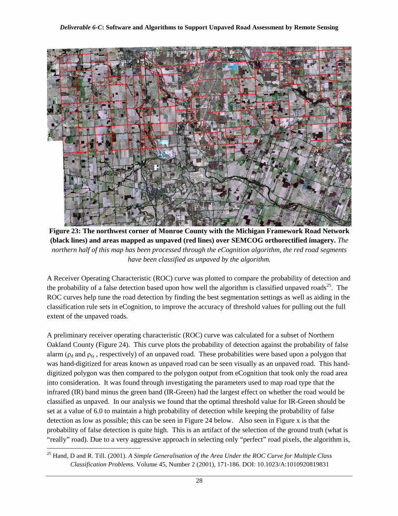
Figure 23: The northwest corner of Monroe County with the Michigan Framework Road Network (black lines) and areas mapped as unpaved (red lines) over SEMCOG orthorectified imagery. The northern half of this map has been processed through the eCognition algorithm, the red road segments

have been classified as unpaved by the algorithm. A Receiver Operating Characteristic (ROC) curve was plotted to compare the probability of detection and the probability of a false detection based upon how well the algorithm is classified unpaved roads25

. The ROC curves help tune the road detection by finding the best segmentation settings as well as aiding in the classification rule sets in eCognition, to improve the accuracy of threshold values for pulling out the full extent of the unpaved roads.

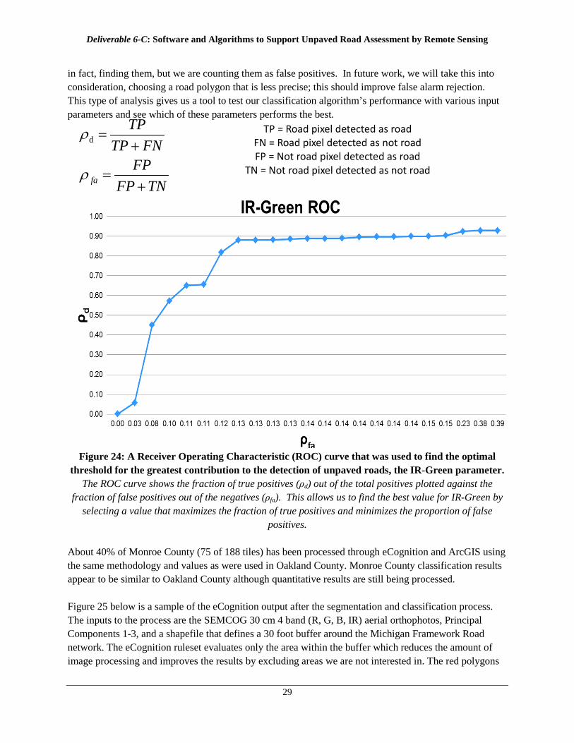
A preliminary receiver operating characteristic (ROC) curve was calculated for a subset of Northern Oakland County (Figure 24). This curve plots the probability of detection against the probability of false alarm (ρd and ρfa , respectively) of an unpaved road. These probabilities were based upon a polygon that was hand-digitized for areas known as unpaved road can be seen visually as an unpaved road. This hand-digitized polygon was then compared to the polygon output from eCognition that took only the road area into consideration. It was found through investigating the parameters used to map road type that the infrared (IR) band minus the green band (IR-Green) had the largest effect on whether the road would be classified as unpaved. In our analysis we found that the optimal threshold value for IR-Green should be set at a value of 6.0 to maintain a high probability of detection while keeping the probability of false detection as low as possible; this can be seen in Figure 24 below. Also seen in Figure x is that the probability of false detection is quite high. This is an artifact of the selection of the ground truth (what is “really” road). Due to a very aggressive approach in selecting only “perfect” road pixels, the algorithm is, 25 Hand, D and R. Till. (2001). A Simple Generalisation of the Area Under the ROC Curve for Multiple Class

Classification Problems. Volume 45, Number 2 (2001), 171-186. DOI: 10.1023/A:1010920819831


29

in fact, finding them, but we are counting them as false positives. In future work, we will take this into consideration, choosing a road polygon that is less precise; this should improve false alarm rejection. This type of analysis gives us a tool to test our classification algorithm’s performance with various input parameters and see which of these parameters performs the best.

Figure 24: A Receiver Operating Characteristic (ROC) curve that was used to find the optimal

threshold for the greatest contribution to the detection of unpaved roads, the IR-Green parameter. The ROC curve shows the fraction of true positives (ρd) out of the total positives plotted against the

fraction of false positives out of the negatives (ρfa). This allows us to find the best value for IR-Green by selecting a value that maximizes the fraction of true positives and minimizes the proportion of false

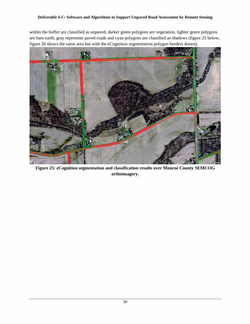
positives. About 40% of Monroe County (75 of 188 tiles) has been processed through eCognition and ArcGIS using the same methodology and values as were used in Oakland County. Monroe County classification results appear to be similar to Oakland County although quantitative results are still being processed. Figure 25 below is a sample of the eCognition output after the segmentation and classification process. The inputs to the process are the SEMCOG 30 cm 4 band (R, G, B, IR) aerial orthophotos, Principal Components 1-3, and a shapefile that defines a 30 foot buffer around the Michigan Framework Road network. The eCognition ruleset evaluates only the area within the buffer which reduces the amount of image processing and improves the results by excluding areas we are not interested in. The red polygons

TNFPFP

FNTPTP

fa +=

+=

ρ

ρdTP = Road pixel detected as road

FN = Road pixel detected as not road FP = Not road pixel detected as road

TN = Not road pixel detected as not road


30

within the buffer are classified as unpaved, darker green polygons are vegetation, lighter green polygons are bare earth, gray represents paved roads and cyan polygons are classified as shadows (figure 25 below; figure 26 shows the same area but with the eCognition segmentation polygon borders drawn).

Figure 25: eCognition segmentation and classification results over Monroe County SEMCOG

orthoimagery.


31

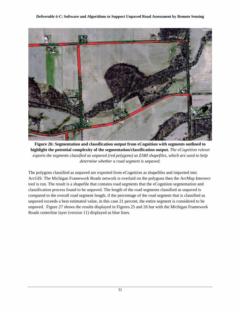
Figure 26: Segmentation and classification output from eCognition with segments outlined to

highlight the potential complexity of the segmentation/classification output. The eCognition ruleset exports the segments classified as unpaved (red polygons) as ESRI shapefiles, which are used to help

determine whether a road segment is unpaved. The polygons classified as unpaved are exported from eCognition as shapefiles and imported into ArcGIS. The Michigan Framework Roads network is overlaid on the polygons then the ArcMap Intersect tool is run. The result is a shapefile that contains road segments that the eCognition segmentation and classification process found to be unpaved. The length of the road segments classified as unpaved is compared to the overall road segment length, if the percentage of the road segment that is classified as unpaved exceeds a best estimated value, in this case 21 percent, the entire segment is considered to be unpaved. Figure 27 shows the results displayed in Figures 25 and 26 but with the Michigan Framework Roads centerline layer (version 11) displayed as blue lines.


32

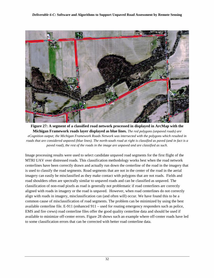
Figure 27: A segment of a classified road network processed in displayed in ArcMap with the

Michigan Framework roads layer displayed as blue lines. The red polygons (unpaved roads) are eCognition output; the Michigan Framework Roads Network was intersected with the polygons which resulted in

roads that are considered unpaved (blue lines). The north-south road at right is classified as paved (and in fact is a paved road), the rest of the roads in the image are unpaved and are classified as such.

Image processing results were used to select candidate unpaved road segments for the first flight of the MTRI UAV over distressed roads. This classification methodology works best when the road network centerlines have been correctly drawn and actually run down the centerline of the road in the imagery that is used to classify the road segments. Road segments that are not in the center of the road in the aerial imagery can easily be misclassified as they make contact with polygons that are not roads. Fields and road shoulders often are spectrally similar to unpaved roads and can be classified as unpaved. The classification of non-road pixels as road is generally not problematic if road centerlines are correctly aligned with roads in imagery or the road is unpaved. However, when road centerlines do not correctly align with roads in imagery, misclassification can (and often will) occur. We have found this to be a common cause of misclassification of road segments. The problem can be minimized by using the best available centerline file. E-911 (enhanced 911 – used for routing emergency responders such as police, EMS and fire crews) road centerline files offer the good quality centerline data and should be used if available to minimize off-center errors. Figure 28 shows such an example where off-center roads have led to some classification errors that can be corrected with better road centerline data.


33

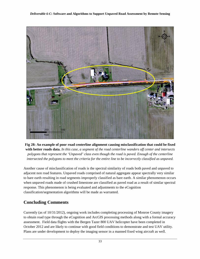
Fig 28: An example of poor road centerline alignment causing misclassification that could be fixed with better roads data. In this case, a segment of the road centerline wanders off center and intersects

polygons that represent the ‘Unpaved’ class even though the road is paved. Enough of the centerline intersected the polygons to meet the criteria for the entire line to be incorrectly classified as unpaved.

Another cause of misclassification of roads is the spectral similarity of roads both paved and unpaved to adjacent non road features. Unpaved roads comprised of natural aggregate appear spectrally very similar to bare earth resulting in road segments improperly classified as bare earth. A similar phenomenon occurs when unpaved roads made of crushed limestone are classified as paved road as a result of similar spectral response. This phenomenon is being evaluated and adjustments to the eCognition classification/segmentation algorithms will be made as warranted. Concluding Comments Currently (as of 10/31/2012), ongoing work includes completing processing of Monroe County imagery to obtain road type through the eCognition and ArcGIS processing methods along with a formal accuracy assessment. Field data flights with the Bergen Tazer 800 UAV helicopter have been completed in October 2012 and are likely to continue with good field conditions to demonstrate and test UAV utility. Plans are under development to deploy the imaging sensor in a manned fixed wing aircraft as well.


34

Imagery taken during these flights is being processed into usable unpaved road condition indicators and will be integrated into RoadSoft DSS demonstrations of unpaved road management.


35

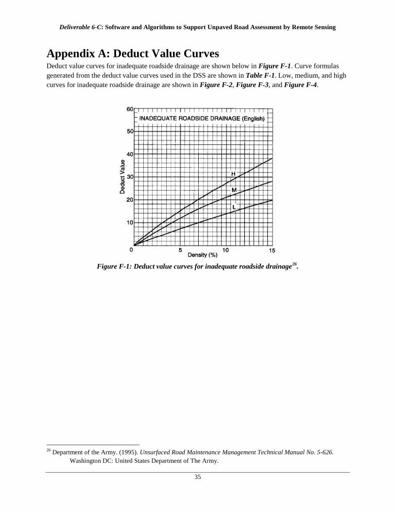
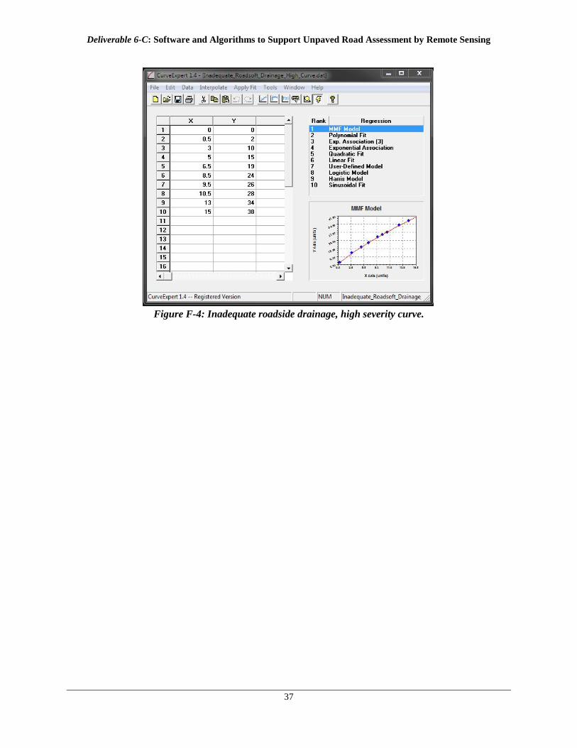
Appendix A: Deduct Value Curves Deduct value curves for inadequate roadside drainage are shown below in Figure F-1. Curve formulas generated from the deduct value curves used in the DSS are shown in Table F-1. Low, medium, and high curves for inadequate roadside drainage are shown in Figure F-2, Figure F-3, and Figure F-4.

Figure F-1: Deduct value curves for inadequate roadside drainage26



.


36

Figure F-2: Inadequate roadside drainage, low severity curve.

Figure F-3: Inadequate roadside drainage, medium severity curve.


37

Figure F-4: Inadequate roadside drainage, high severity curve.


38

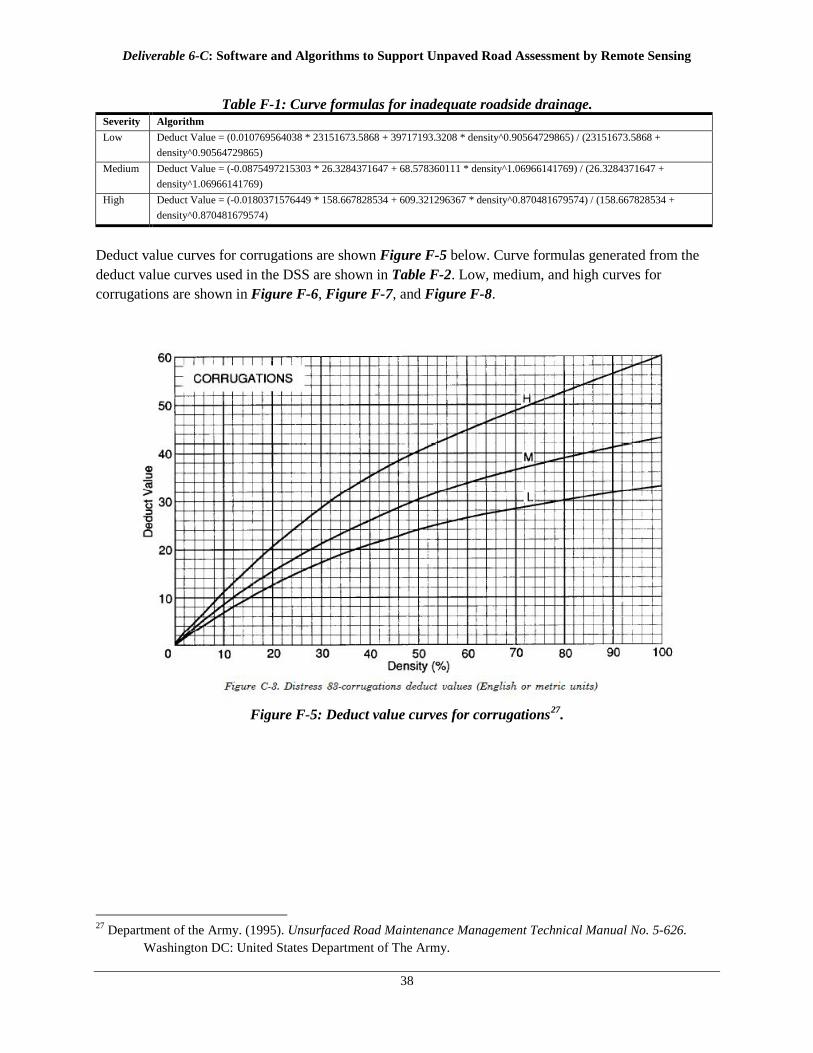
Table F-1: Curve formulas for inadequate roadside drainage. Severity Algorithm Low Deduct Value = (0.010769564038 * 23151673.5868 + 39717193.3208 * density^0.90564729865) / (23151673.5868 +

density^0.90564729865) Medium Deduct Value = (-0.0875497215303 * 26.3284371647 + 68.578360111 * density^1.06966141769) / (26.3284371647 +

density^1.06966141769) High Deduct Value = (-0.0180371576449 * 158.667828534 + 609.321296367 * density^0.870481679574) / (158.667828534 +

density^0.870481679574)

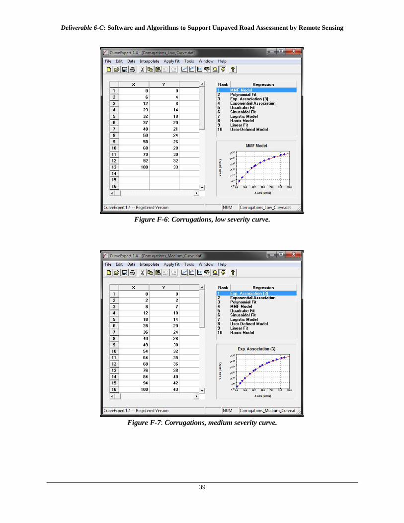
Deduct value curves for corrugations are shown Figure F-5 below. Curve formulas generated from the deduct value curves used in the DSS are shown in Table F-2. Low, medium, and high curves for corrugations are shown in Figure F-6, Figure F-7, and Figure F-8.

Figure F-5: Deduct value curves for corrugations27

.




39

Figure F-6: Corrugations, low severity curve.

Figure F-7: Corrugations, medium severity curve.


40

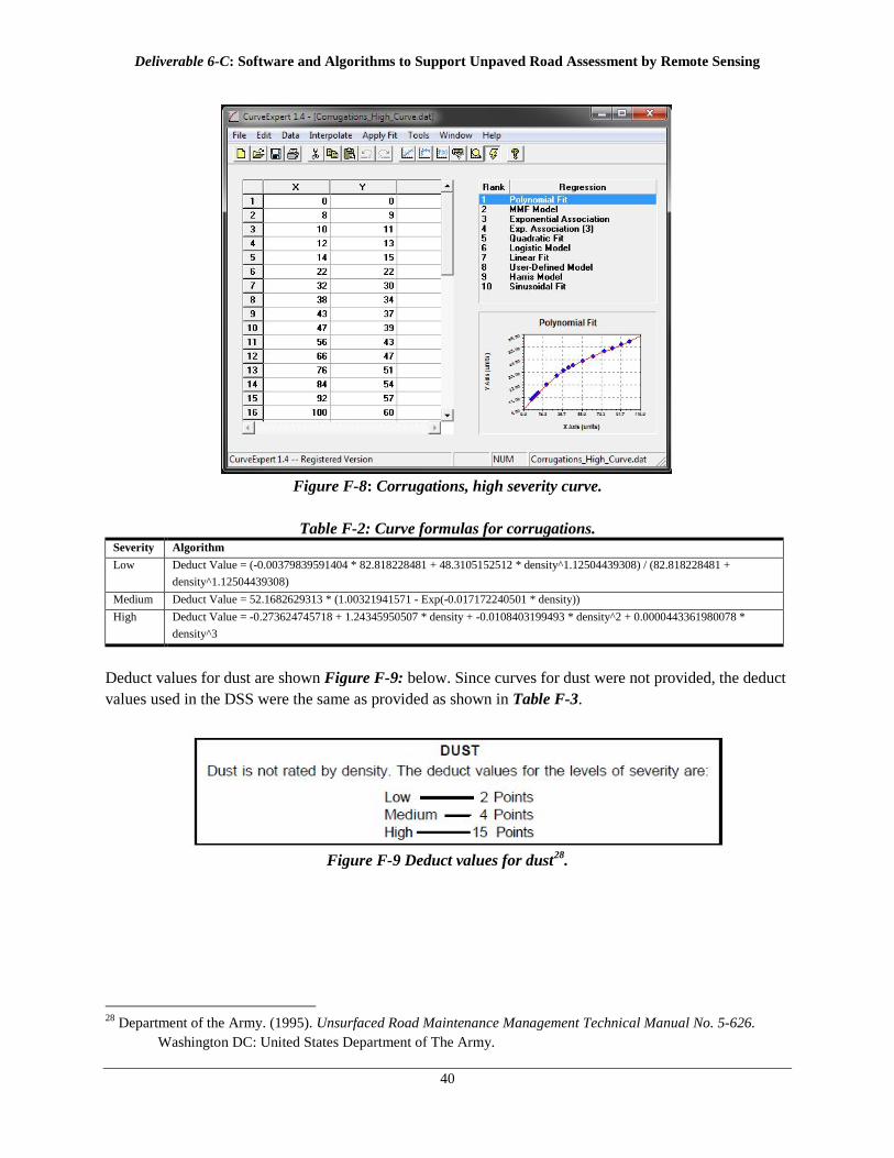
Figure F-8: Corrugations, high severity curve.

Table F-2: Curve formulas for corrugations.

Severity Algorithm Low Deduct Value = (-0.00379839591404 * 82.818228481 + 48.3105152512 * density^1.12504439308) / (82.818228481 +

density^1.12504439308) Medium Deduct Value = 52.1682629313 * (1.00321941571 - Exp(-0.017172240501 * density)) High Deduct Value = -0.273624745718 + 1.24345950507 * density + -0.0108403199493 * density^2 + 0.0000443361980078 *

density^3

Deduct values for dust are shown Figure F-9: below. Since curves for dust were not provided, the deduct values used in the DSS were the same as provided as shown in Table F-3.

Figure F-9 Deduct values for dust28

.




41

Table F-3: Deduct values for dust. Severity Algorithm Low Deduct Value = 2 Medium Deduct Value = 4 High Deduct Value = 15

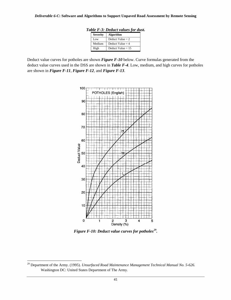
Deduct value curves for potholes are shown Figure F-10 below. Curve formulas generated from the deduct value curves used in the DSS are shown in Table F-4. Low, medium, and high curves for potholes are shown in Figure F-11, Figure F-12, and Figure F-13.

Figure F-10: Deduct value curves for potholes29

.




42

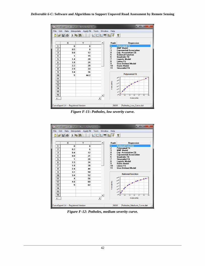
Figure F-11: Potholes, low severity curve.

Figure F-12: Potholes, medium severity curve.


43

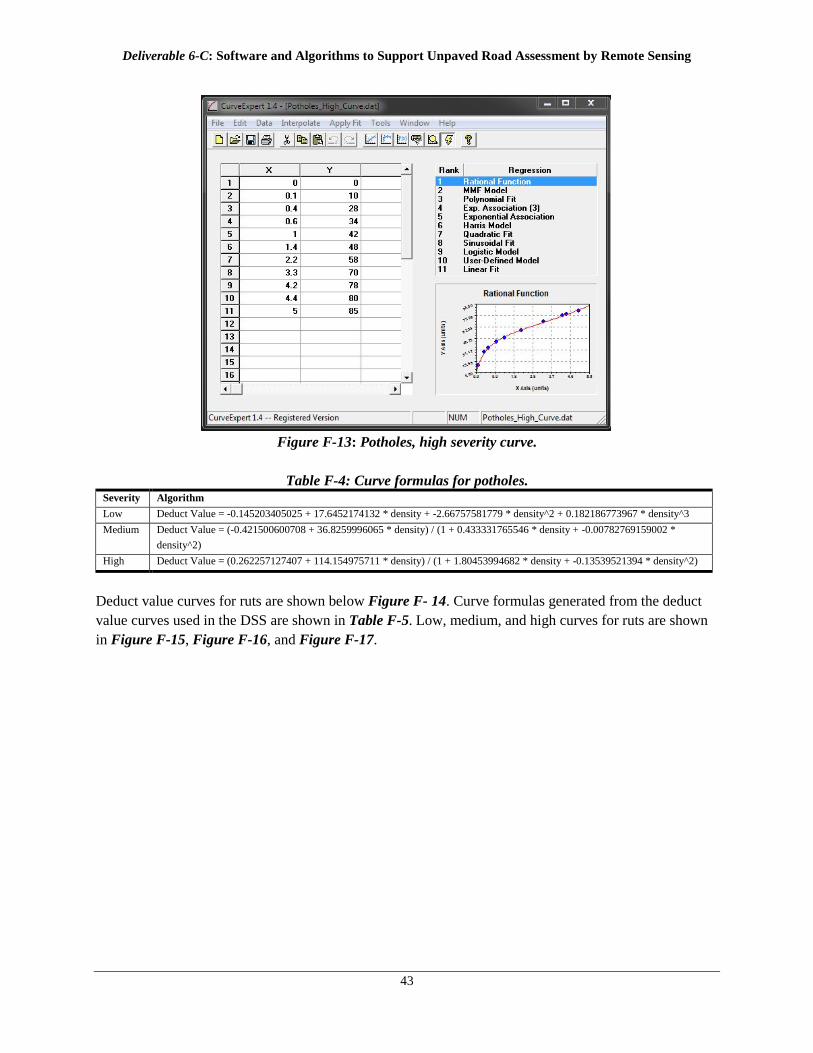
Figure F-13: Potholes, high severity curve.

Table F-4: Curve formulas for potholes.

Severity Algorithm Low Deduct Value = -0.145203405025 + 17.6452174132 * density + -2.66757581779 * density^2 + 0.182186773967 * density^3 Medium Deduct Value = (-0.421500600708 + 36.8259996065 * density) / (1 + 0.433331765546 * density + -0.00782769159002 *

density^2) High Deduct Value = (0.262257127407 + 114.154975711 * density) / (1 + 1.80453994682 * density + -0.13539521394 * density^2)

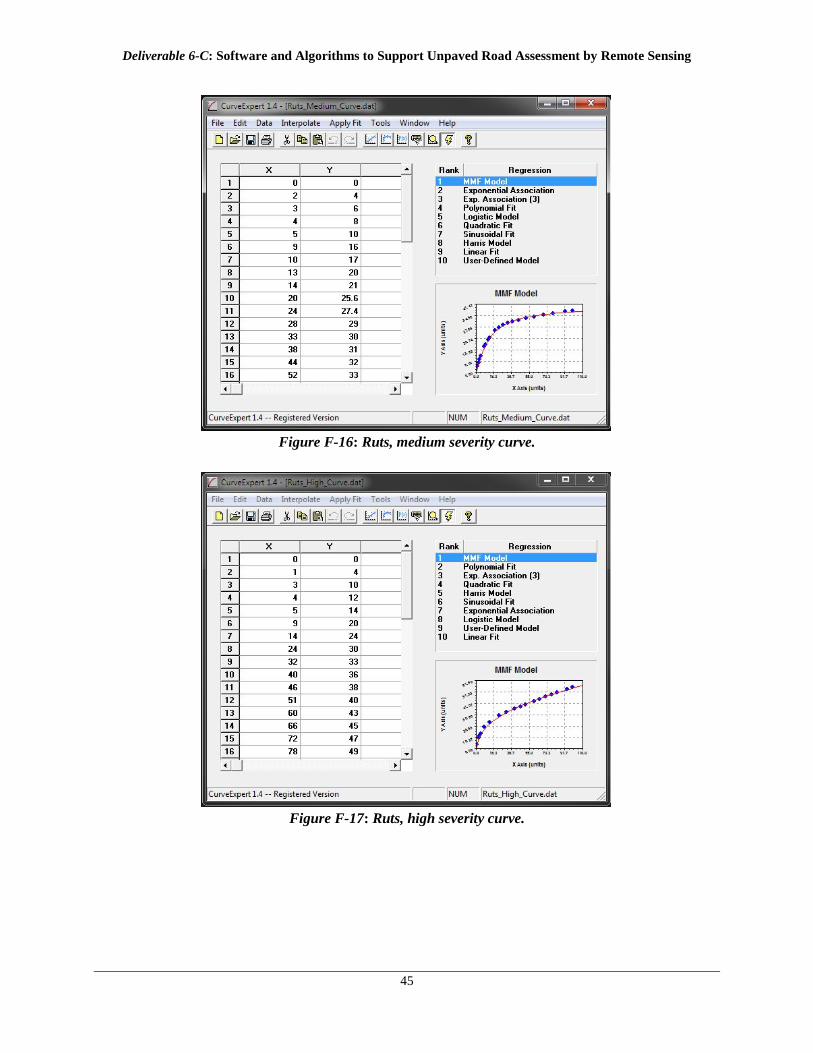
Deduct value curves for ruts are shown below Figure F- 14. Curve formulas generated from the deduct value curves used in the DSS are shown in Table F-5. Low, medium, and high curves for ruts are shown in Figure F-15, Figure F-16, and Figure F-17.


44

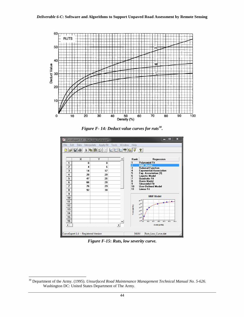
Figure F- 14: Deduct value curves for ruts30

.

Figure F-15: Ruts, low severity curve.




45

Figure F-16: Ruts, medium severity curve.

Figure F-17: Ruts, high severity curve.


46

Table F-6: Curve formulas for ruts. Severity Algorithm Low Deduct Value = ((-0.180079645328 * 17.1341777707) + (34.233052738 * density^1.04992408893)) / (17.1341777707 +

density^1.04992408893) Medium Deduct Value = ((-0.0886072180049 * 19.4773810794) + (40.4131963046 * density^1.15633948131)) / (19.4773810794 +

density^1.15633948131) High Deduct Value = ((-0.785806790035 * 86.5215401586) + (600.859004333 * density^0.472634159393)) / (86.5215401586 +

density^0.472634159393)

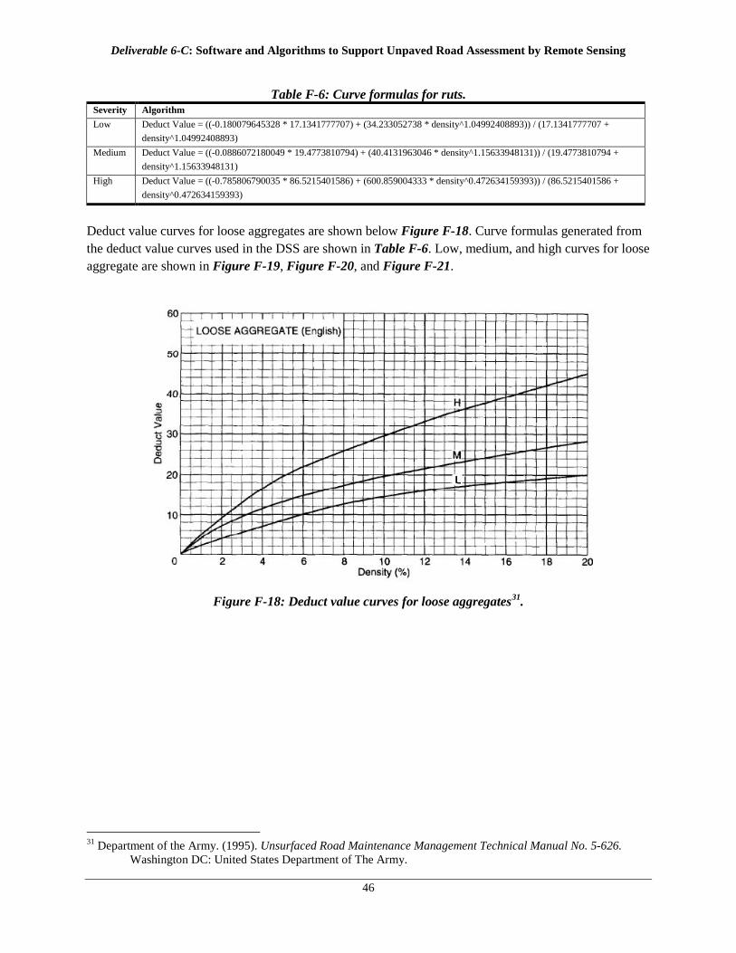
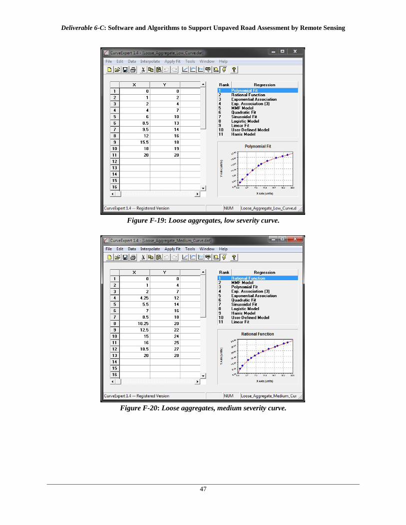
Deduct value curves for loose aggregates are shown below Figure F-18. Curve formulas generated from the deduct value curves used in the DSS are shown in Table F-6. Low, medium, and high curves for loose aggregate are shown in Figure F-19, Figure F-20, and Figure F-21.

Figure F-18: Deduct value curves for loose aggregates31

.




47

Figure F-19: Loose aggregates, low severity curve.

Figure F-20: Loose aggregates, medium severity curve.


48

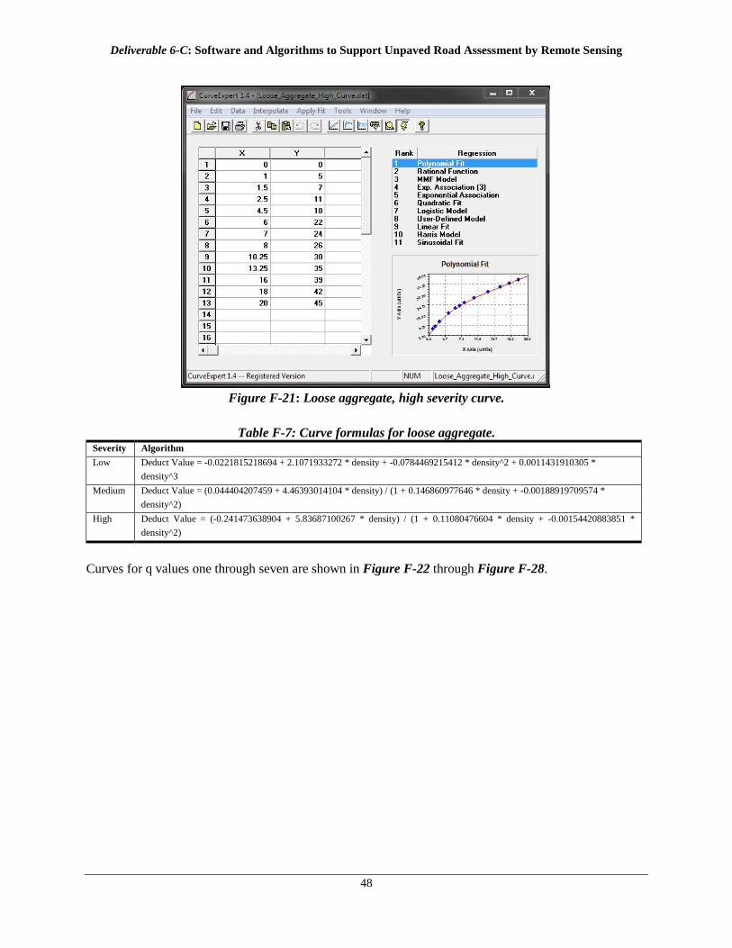
Figure F-21: Loose aggregate, high severity curve.

Table F-7: Curve formulas for loose aggregate.

Severity Algorithm Low Deduct Value = -0.0221815218694 + 2.1071933272 * density + -0.0784469215412 * density^2 + 0.0011431910305 *

density^3 Medium Deduct Value = (0.044404207459 + 4.46393014104 * density) / (1 + 0.146860977646 * density + -0.00188919709574 *

density^2) High Deduct Value = (-0.241473638904 + 5.83687100267 * density) / (1 + 0.11080476604 * density + -0.00154420883851 *

density^2)

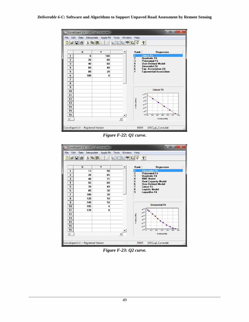
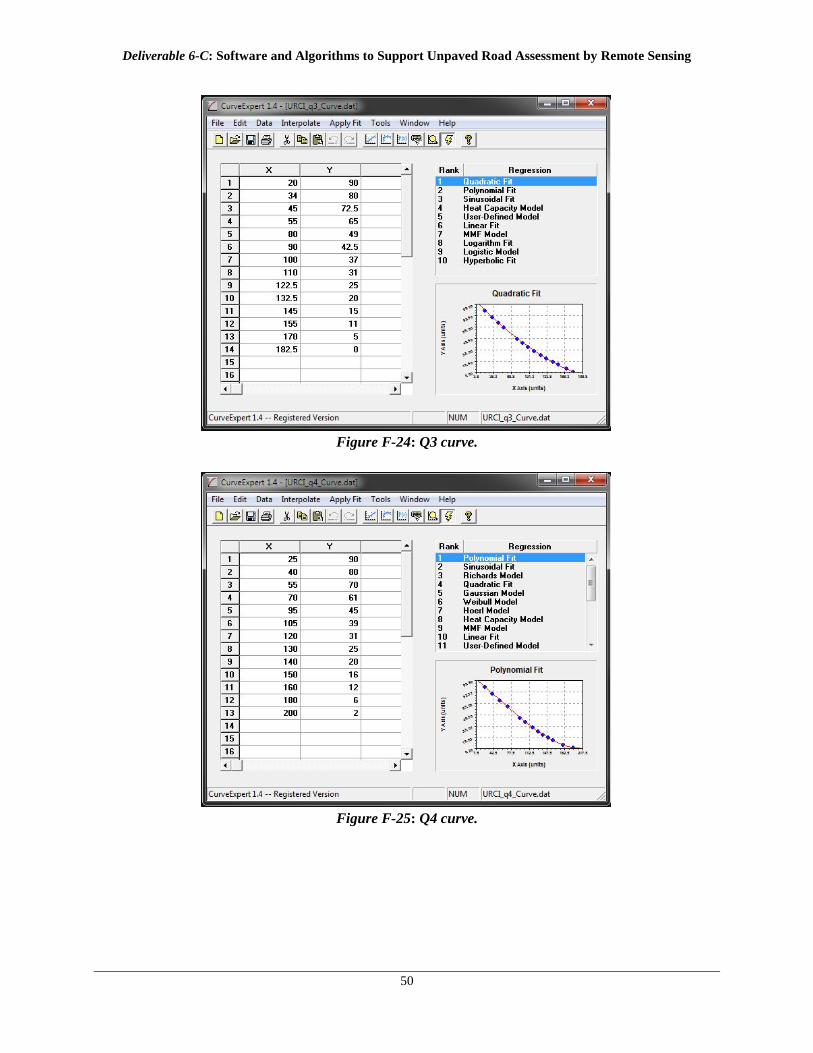
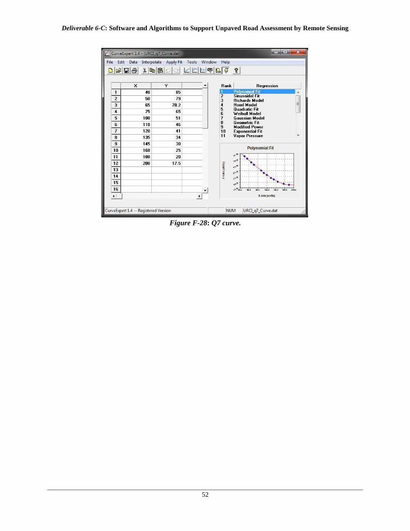
Curves for q values one through seven are shown in Figure F-22 through Figure F-28.


49

Figure F-22: Q1 curve.



50




51




52


Documents

Deliverable 6-C: Software and Algorithms to Support ... · . 3 Colling, T., & Schlaff, G. (2012)