Embed Size (px)
Citation preview

R E
OC N
F I G
ICT Call 9RECONFIG
FP7-ICT-600825
Deliverable D3.4:
Strengthening robustness
August 26, 2015

D3.4 FP7-ICT-600825 RECONFIG August 26, 2015
Project acronym: RECONFIGProject full title: Cognitive, Decentralized Coordination of Heterogeneous
Multi-Robot Systems via Reconfigurable Task Planning
Work Package: WP3Document number: D3.4Document title: Strengthening robustnessVersion: 1.0
Delivery date: August 31, 2015Nature: ReportDissemination level: Internal
Authors: Charalampos P. Bechlioulis (NTUA)George C. Karras (NTUA)Kostas J. Kyriakopoulos (NTUA)
The research leading to these results has received funding from the European Union SeventhFramework Programme FP7/2007-2013 under grant agreement no600825 RECONFIG.
2
Contents
1 Introduction 21.1 Robust Transportation via Implicit Communication . . . . . . . . . . . . . . . . 21.2 Fault Tolerant Control for Omni-directional Platforms . . . . . . . . . . . . . . . 31.3 Robust Cooperation for Multi-Agent Systems . . . . . . . . . . . . . . . . . . . 41.4 Summary . . . . . . . . . . . . . . . . . . . . . . . . . . . . . . . . . . . . . . . 51.5 Future Research Directions . . . . . . . . . . . . . . . . . . . . . . . . . . . . . 6
2 Robust Transportation via Implicit Communication 72.1 Problem formulation . . . . . . . . . . . . . . . . . . . . . . . . . . . . . . . . . 7
2.1.1 Kinematics . . . . . . . . . . . . . . . . . . . . . . . . . . . . . . . . . . 82.1.2 Dynamics . . . . . . . . . . . . . . . . . . . . . . . . . . . . . . . . . . 8
2.2 Control Methodology . . . . . . . . . . . . . . . . . . . . . . . . . . . . . . . . 92.2.1 Leader’s Control Scheme . . . . . . . . . . . . . . . . . . . . . . . . . . 102.2.2 Follower’s Control Scheme . . . . . . . . . . . . . . . . . . . . . . . . . 12
2.3 Simulations . . . . . . . . . . . . . . . . . . . . . . . . . . . . . . . . . . . . . 16
3 Fault Tolerant Control for Omni-directional Platforms 223.1 Problem formulation . . . . . . . . . . . . . . . . . . . . . . . . . . . . . . . . . 22
3.1.1 Vehicle Kinematics . . . . . . . . . . . . . . . . . . . . . . . . . . . . . 233.1.2 Vehicle Dynamics . . . . . . . . . . . . . . . . . . . . . . . . . . . . . . 253.1.3 Problem statement . . . . . . . . . . . . . . . . . . . . . . . . . . . . . 25
3.2 Fault Tolerant Control . . . . . . . . . . . . . . . . . . . . . . . . . . . . . . . . 263.2.1 No Faulty Wheels . . . . . . . . . . . . . . . . . . . . . . . . . . . . . . 263.2.2 One Faulty Wheel . . . . . . . . . . . . . . . . . . . . . . . . . . . . . . 283.2.3 Two Faulty Wheels . . . . . . . . . . . . . . . . . . . . . . . . . . . . . 28
3.3 Experimental Results . . . . . . . . . . . . . . . . . . . . . . . . . . . . . . . . 31
4 Robust Cooperation for Multi-Agent Systems 384.1 Problem Formulation and Preliminaries . . . . . . . . . . . . . . . . . . . . . . . 384.2 Main Results . . . . . . . . . . . . . . . . . . . . . . . . . . . . . . . . . . . . . 40
4.2.1 Sufficient Conditions . . . . . . . . . . . . . . . . . . . . . . . . . . . . 404.2.2 Distributed Control Protocol . . . . . . . . . . . . . . . . . . . . . . . . 44
4.3 Simulation Results . . . . . . . . . . . . . . . . . . . . . . . . . . . . . . . . . . 51
Appendix A 63
3

D3.4 FP7-ICT-600825 RECONFIG August 26, 2015
Appendix B 65
4
Abstract
Owing to environmental as well as goal uncertainties, possible failures and limited resources, robustclosed loop systems have to be developed. Therefore, the robustness is expected to be examined inview of the new task parametrization derived from the implicit/sensor based and explicit/symboliccommunication, considered within the RECONFIG project. Towards this direction, the goal ofthis deliverable is the reinforcement of the closed loop robustness against system uncertainties,actuator failures and limited resources. Finally, this deliverable contributes to both MilestonesMS.2 and MS.3 by strengthening the robustness of the proposed framework against uncertaintiesand actuator faults.
Chapter 1Introduction
Decentralized multi-agent systems have recently emerged as an inexpensive and robust way ofaddressing a wide variety of tasks ranging from exploration, surveillance, and reconnaissance tocooperative construction and manipulation. Using a group of robots instead of a single one yieldsseveral advantages, such as increase in capabilities, increase of redundancy and versatility andfault tolerance. The success of decentralized multi-agent systems relies on efficient informationexchange and coordination between the members of the team. More specifically, their intriguingfeature consists on the fact that each agent makes decisions solely on the basis of its localperception of the environment, which has also been observed in many biological systems [1].Thus, a challenging task is to design decentralized control protocols for certain global goals in thepresence of limited information exchange, system uncertainties and actuator faults.
1.1 Robust Transportation via Implicit Communication
In general, there are two types of communication, namely the explicit and the implicit. Theformer type is designed solely to convey information such as control signals or sensory data directlyto other robots [2]. On the other hand, the latter occurs as a side-effect of robot’s interactions withthe environment or other robots, either physically (e.g., the interaction forces between the objectand the robot) or non-physically (e.g., visual observation). In this case, the information neededis acquired by appropriate sensors attached on the agents. The most investigated and frequentlyemployed communication form is the explicit one. It usually leads to simpler theoretic analysisand renders teams more effective. However, in case of faulty communication environments, severeproblems may arise, such as dropping the object, exertion of excessive forces and performancedegradation. Moreover, as the number of cooperating robots increases, communication protocolsrequire complex design to deal with crowded bandwidth [3]. On the other hand, several ofthe aforementioned limitations can be overcome by employing implicit communication instead.Despite the increased difficulty of the theoretical analysis, it leads to simpler protocols and savesbandwidth as well as power, since no or very few data is explicitly exchanged. Furthermore, itsignificantly increases robustness in case of faulty environments as well as stealthiness of operation,since the agent activity is not easily detected. One may argue though, that the explicit form leads,when accurately employed, to superior performances. Nevertheless, there are tasks, for which itis not essential, especially when the implicit form is available. It should also be noticed that morecomplex communication networks may offer little or no benefit over implicit communication [4,5].
Cooperative transportation has been well-studied in the literature, especially the centralized
2
D3.4 FP7-ICT-600825 RECONFIG August 26, 2015
schemes [6–9]. Despite its efficiency, centralized control is less robust, since all units rely on acentral system, and its complexity increases rapidly as the number of participating robots becomeslarge. On the other hand, decentralized control usually depends on either explicit communicationor off-line knowledge of the desired object trajectory [10–12]. Moreover, in other leader-followerschemes [13,14], the leader has to transmit on-line the desired object trajectory to the follower.
Implicit communication has been exclusively employed in a few decentralized schemes forholonomic mobile manipulators. Kosuge et. al. in a series of works [15–17] presented a leader-follower scheme for holonomic manipulators. The leader implements a desired trajectory profilethrough an impedance scheme, while the follower estimates it through the motion of the object.However, the dynamics of the object are neglected and the estimation error remains boundedclose to zero only if the desired acceleration is zero (i.e., trajectories with constant velocity profile).Finally, regarding non-holonomic mobile robots, the follower’s passive caster behavior was adoptedin [18,19]. Although, the stability of the follower’s contact is established, it is not stated how theobject’s trajectory can be controlled.
1.2 Fault Tolerant Control for Omni-directional Platforms
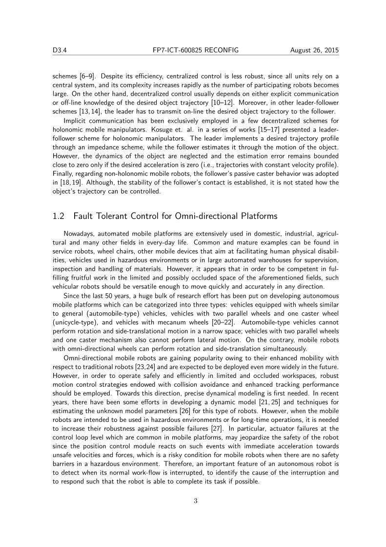
Nowadays, automated mobile platforms are extensively used in domestic, industrial, agricul-tural and many other fields in every-day life. Common and mature examples can be found inservice robots, wheel chairs, other mobile devices that aim at facilitating human physical disabil-ities, vehicles used in hazardous environments or in large automated warehouses for supervision,inspection and handling of materials. However, it appears that in order to be competent in ful-filling fruitful work in the limited and possibly occluded space of the aforementioned fields, suchvehicular robots should be versatile enough to move quickly and accurately in any direction.
Since the last 50 years, a huge bulk of research effort has been put on developing autonomousmobile platforms which can be categorized into three types: vehicles equipped with wheels similarto general (automobile-type) vehicles, vehicles with two parallel wheels and one caster wheel(unicycle-type), and vehicles with mecanum wheels [20–22]. Automobile-type vehicles cannotperform rotation and side-translational motion in a narrow space; vehicles with two parallel wheelsand one caster mechanism also cannot perform lateral motion. On the contrary, mobile robotswith omni-directional wheels can perform rotation and side-translation simultaneously.
Omni-directional mobile robots are gaining popularity owing to their enhanced mobility withrespect to traditional robots [23,24] and are expected to be deployed even more widely in the future.However, in order to operate safely and efficiently in limited and occluded workspaces, robustmotion control strategies endowed with collision avoidance and enhanced tracking performanceshould be employed. Towards this direction, precise dynamical modeling is first needed. In recentyears, there have been some efforts in developing a dynamic model [21, 25] and techniques forestimating the unknown model parameters [26] for this type of robots. However, when the mobilerobots are intended to be used in hazardous environments or for long-time operations, it is neededto increase their robustness against possible failures [27]. In particular, actuator failures at thecontrol loop level which are common in mobile platforms, may jeopardize the safety of the robotsince the position control module reacts on such events with immediate acceleration towardsunsafe velocities and forces, which is a risky condition for mobile robots when there are no safetybarriers in a hazardous environment. Therefore, an important feature of an autonomous robot isto detect when its normal work-flow is interrupted, to identify the cause of the interruption andto respond such that the robot is able to complete its task if possible.
3
D3.4 FP7-ICT-600825 RECONFIG August 26, 2015
In particular, four-wheeled omni-directional mobile robots have the relevant characteristic thatthey can still operate with three wheels in case some malfunctioning in one wheel has beendetected. This makes them good setups for testing techniques that provide fault tolerance againstactuator faults. The objective of a fault-tolerant control (FTC) system [28] is to maintain currentperformances close to desirable ones and preserve stability conditions in the presence of faults.The existing design techniques mainly include the passive and the active approach [29, 30]. Thepassive FTC techniques take into account the fault as a system perturbation, such that the controllaw is designed to have inherent fault tolerance capabilities. On the other hand, the active FTCtechniques try to satisfy the control objectives with minimum performance degradation either byselecting a precalculated control law or by synthesizing online a new control strategy.
1.3 Robust Cooperation for Multi-Agent Systems
Although the majority of the works on distributed cooperative control consider known andsimple dynamic models, many practical engineering systems exist that fail to satisfy that assump-tion and which moreover are constantly subject to environmental disturbances. Thus, taking intoaccount the inherent model uncertainties when designing robust distributed control schemes isof paramount importance. Extending towards this direction, existing control techniques for idealmodels, such as linear control theory [31–35], H∞ control [36–39] or internal model principal[40–44], becomes a very challenging task on account of the increasing design complexity owingto the interacting system dynamics as reflected by the local intercourse specifications.
Attempts to address the multi-agent consensus/synchronization/formation control for sys-tems with unknown nonlinear dynamics and disturbances were presented in [45–54] employingneuro/fuzzy approximating structures. Unfortunately, the aforementioned schemes inherently in-troduce certain issues affecting closed loop stability and robustness. Specifically, even though theexistence of a closed loop initialization set as well as of control gain values that guarantee closedloop stability can be proven, the problem of proposing an explicit constructive methodology capa-ble of a priori imposing the required stability properties is not addressed. As a consequence, theproduced control schemes yield inevitably reduced levels of robustness against modeling imperfec-tions. Moreover, the results are restricted to be local as they are valid only within the compactset where the capabilities of the universal approximators hold. Furthermore, the introduction ofapproximating structures increases the complexity of the proposed control schemes in the sensethat extra adaptive parameters have to be updated (i.e., extra nonlinear differential equationshave to be solved numerically) and extra calculations have to be conducted to output the controlsignal, thus making their distributed implementation difficult. Alternatively, in case upper boundson the magnitude of the model uncertainties are available, approximation-free approaches havebeen proposed in [55–59] based on the sliding mode control technique. However, sliding modecontrol leads inevitably to chattering near the sliding surface, which is undesirable since it involveshigh control activity and may further excite unmodeled high frequency dynamics.
Another important issue associated with decentralized cooperative control schemes of multi-agent systems under model uncertainties, concerns the transient and steady state response ofthe closed loop system. Traditionally, the synchronization/consensus error is proven to convergewithin a residual set, whose size depends on control design parameters and some unknown (thoughbounded) terms. However, no systematic procedure exists to accurately compute the requiredupper bounds, thus making the a priori selection of the aforementioned control parameters tosatisfy certain steady state behavior, practically impossible. Moreover, transient behavior (i.e., the
4
D3.4 FP7-ICT-600825 RECONFIG August 26, 2015
convergence rate) is difficult to establish analytically as it is affected heavily by the agents’ modeldynamics and the status of the overall underlying interaction topology, both of which are consideredunknown. The transient performance problem was relaxed for single integrator multi-agent systemsunder undirected communication graph in [60], following the notion of prescribed performancecontrol [61]. Additionally, a few works [62,63] have also appeared aiming at establishing increasedlevels of quality in the transient response, via minimizing certain performance indices. However,the aforementioned performance indices are connected only indirectly with the actual systemresponse. Although reducing them may result in an overall transient performance improvement,no specific connection to a priori determined trajectory oriented metrics can be obtained.
1.4 Summary
In Chapter 2, we address the problem of decentralized cooperative object transportation ina constrained workspace with static obstacles. The challenge lies in completely replacing explicitcommunication with implicit, that results indirectly from the physical interaction of the robots viathe commonly carried object (i.e., as the robots move, forces and torques are exerted in certaindirections at the robot/object contacts). Similarly to [17], the considered architecture is a leader-follower scheme. The leader is aware of both the object’s desired configuration as well as of theposition of the obstacles in the workspace and employs a Navigation Function based scheme toachieve the object’s desired configuration and avoid collisions with the obstacles and the workspaceboundary. The follower, that does not know the object’s goal configuration, estimates it byobserving its motion. The estimation process is based on the prescribed performance methodology[64] that drives the estimation error to an arbitrarily small residual set. The robots employadaptive laws to compensate for the parametric uncertainty of their dynamic models. Finally, itshould be noticed that both agents use solely their own force, position and velocity measurements,avoiding thus any inter-robot explicit communication. In this work, Navigation Functions [65] areinnovatively incorporated with adaptive control techniques to deal with the parametric uncertaintyin the robot dynamics, extending thus greatly the current state of the art in robust motion planningand collision avoidance by studying second order dynamics with parametric uncertainty. We alsoextend the current state of art [15–17], via a more robust estimation algorithm that convergeseven though the desired object’s acceleration profile is non-zero (i.e., arbitrary object’s desiredtrajectory profile as long as it is bounded and smooth). Moreover, the customizable ultimatebounds allow us to achieve practical stabilization of the estimation error, with accuracy limitedonly by the sensors’ resolution.
In Chapter 3, we address the fault tolerant control problem for an omni-directional mobileplatform with four mecanum wheels in a constrained workspace with static obstacles. The chal-lenge with respect to the current state of the art in fault tolerant control for such mobile platforms,where only one faulted wheel is considered (i.e., the platform still retains its full actuation ca-pabilities), lies in completely compensating up to two faulted wheels (i.e., the model becomesunderactuated) despite the dynamic model uncertainty and the presence of static obstacles in theworkspace. In this work, both conventional and dipolar Navigation Functions [65, 66] are inno-vatively incorporated with adaptive control techniques to deal with the parametric uncertainty inthe robot dynamics, extending thus greatly the current state of the art in robust motion planningand collision avoidance by studying second order dynamics with parametric uncertainty.
In Chapter 4, a generic class of high-order nonlinear multi-agent systems, under a directedcommunication protocol is considered. A robust, decentralized and approximation-free synchro-
5
D3.4 FP7-ICT-600825 RECONFIG August 26, 2015
nization control scheme is designed in the sense that each agent utilizes only local relative stateinformation from its neighborhood set to calculate its own control signal, without incorporatingany prior knowledge of the model nonlinearities/disturbances or any approximating structures toacquire such knowledge. Additionally, the imposed transient and steady state response bounds aresolely pre-determined by certain designer-specified performance functions and are fully decoupledby the agents’ dynamic model, the underlying graph topology and the control gains selection, re-laxing further the control design procedure. The proposed methodology results in a low complexitysynchronization protocol. Actually, it is a static scheme involving very few and simple calculationsto produce the control signal, thus making its distributed implementation straightforward. Theconcepts and techniques of prescribed performance control methodology, recently developed in[67, 68] for uncertain nonlinear systems, are innovatively adapted in this work to deal with thedecentralized synchronization of unknown high order nonlinear multi-agent systems. In this direc-tion it is stressed that, in all aforementioned works the proposed controllers were designed in acentralized manner owing to the fact that full state feedback was incorporated in the control inputsignals. Hence, since decentralization is mandatory in this work, i.e., each agent should operatesolely on the basis of its local/neighborhood feedback, our previous results cannot be straightfor-wardly applied in the considered control problem, owing to the interacting system dynamics thatare reflected by the local intercourse specifications; thus rendering the contribution of this workwith respect to [61,64,67–69] considerable.
1.5 Future Research Directions
Future research efforts will be devoted towards: i) extending the robust transportation schemein multiple cooperating robots, considering dynamically moving obstacles, ii) extending the faulttolerant control scheme in a dynamic environment with moving obstacles based solely on theodometry (i.e., without employing any external position measurements) and iii) addressing thecollision avoidance and connectivity maintenance problems within multi-agent dynamic communi-cation graphs, retaining the robustness and the prescribed transient and steady state performance.
6
Chapter 2Robust Transportation via Implicit Com-munication
This chapter addresses the problem of cooperative object transportation in a constrainedworkspace involving static obstacles, with the coordination relying solely on implicit communi-cation from the physical interaction of the robots with the object. We consider a decentralizedleader-follower architecture, where the leading robot, that has exclusive knowledge of the object’sdesired configuration and the position of the obstacles in the workspace, tries to navigate theoverall scheme to the goal configuration while avoiding collisions with the obstacles. On the otherhand, the follower estimates the object’s desired trajectory profile via a novel prescribed perfor-mance estimation law, that drives the estimation error to an arbitrarily small residual set. Bothleader and follower employ adaptive laws to handle the parametric uncertainties of their dynamicmodels. The feedback relies exclusively on each robot’s force/torque, position as well as velocitymeasurements and no explicit data is exchanged on-line among the robots, thus reducing therequired communication bandwidth and increasing robustness. Finally, a comparative simulationstudy clarifies the proposed method and verifies its efficiency. The results presented in this chapterwere also included in the submitted conference paper [70].
2.1 Problem formulation
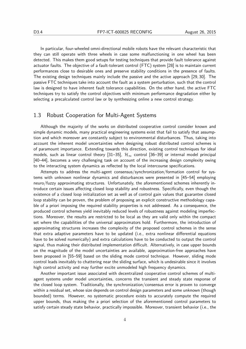
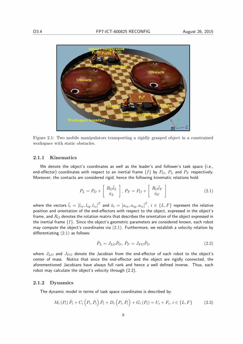
Consider two mobile manipulators in a leader-follower scheme handling a rigidly grasped objectin a constrained workspace with static obstacles, as shown in Fig. 2.1. We assume that eachrobot has at least 6 DoFs and is fully actuated at its end-effector (i.e., any force and torquealong and around all axis of the end-effector’s frame can be applied). It should also be noted thatonly the leading robot is aware of the obstacles’ position in the workspace and the object’s desiredconfiguration P d
O (see Fig. 2.1), whereas the follower should estimate the object’s desired trajectoryprofile via its own state measurements. Moreover, we assume that measurements of position,velocity and interaction forces/torques with the object are available for each robot exclusively.Additionally, the geometric parameters of the mobile manipulators and the grasped object areconsidered known, whereas their dynamic parameters are completely unknown. Finally, noticethat owing to: i) the strict communication constraints (i.e., no on-line inter-robot communicationis permitted), ii) the model uncertainties and iii) the constrained workspace, the problem becomesvery challenging, with no previously reported results in the related literature.
7
D3.4 FP7-ICT-600825 RECONFIG August 26, 2015
Figure 2.1: Two mobile manipulators transporting a rigidly grasped object in a constrainedworkspace with static obstacles.
2.1.1 Kinematics
We denote the object’s coordinates as well as the leader’s and follower’s task space (i.e.,end-effector) coordinates with respect to an inertial frame I by PO, PL and PF respectively.Moreover, the contacts are considered rigid; hence the following kinematic relations hold:
PL = PO +[RO lLaL
], PF = PO +
[RO lFaF
](2.1)
where the vectors li = [lix, liy, liz]T and ai = [aix, aiy, aiz]T , i ∈ L,F represent the relativeposition and orientation of the end-effectors with respect to the object, expressed in the object’sframe, and RO denotes the rotation matrix that describes the orientation of the object expressed inthe inertial frame I. Since the object’s geometric parameters are considered known, each robotmay compute the object’s coordinates via (2.1). Furthermore, we establish a velocity relation bydifferentiating (2.1) as follows:
PL = JLOPO, PF = JF OPO (2.2)
where JLO and JF O denote the Jacobian from the end-effector of each robot to the object’scenter of mass. Notice that since the end-effector and the object are rigidly connected, theaforementioned Jacobians have always full rank and hence a well defined inverse. Thus, eachrobot may calculate the object’s velocity through (2.2).
2.1.2 Dynamics
The dynamic model in terms of task space coordinates is described by:
Mi (Pi) Pi + Ci
(Pi, Pi
)Pi +Di
(Pi, Pi
)+Gi (Pi) = Ui + Fi, i ∈ L,F (2.3)
8
D3.4 FP7-ICT-600825 RECONFIG August 26, 2015
where Mi (Pi), i ∈ L,F denote the positive definite inertial matrices, Ci
(Pi, Pi
), i ∈ L,F
represent coriolis and centrifugal terms, Di
(Pi, Pi
), i ∈ L,F model joint friction effects and
Gi (Pi), i ∈ L,F encapsulate gravitational forces and torques. Furthermore, the vectors Fi, i ∈L,F represent the interaction forces and torques exerted at the end-effector by the object and Ui,i ∈ L,F denote the task space control input wrenches. It is also known that uncertain physicalparameters of the robots, such as link masses and inertias as well as joint friction coefficients,appear linearly in the robot dynamic model (2.3). Hence, we may express the dynamics in termsof a set of unknown but constant parameters θi ∈ ℜQi , i ∈ L,F in the following way:
Mi (a) d+ Ci (a, b) c+Di (a, b) +Gi (a) = ZTi (a, b, c, d) θi, i ∈ L,F (2.4)
where Zi (a, b, c, d), i ∈ L,F are Qi × 6 regressor matrices composed of known nonlinearfunctions. Finally, a skew-symmetric property of the matrices Mi (Pi) − 2Ci
(Pi, Pi
), i ∈ L,F
is also fulfilled.
Remark 1. The relation between the robot joint force/torque control input τi, i ∈ L,F andthe task space control input wrench Ui, i ∈ L,F is given by:
τi = J#Ti Ui +
(I − JT
i J#Ti
)τ0
i , i ∈ L,F (2.5)
where J#i , i ∈ L,F denote the generalized inverse of the robot Jacobians, that is consistent
with the equations of motion of the mobile manipulators’ joints and their end-effectors [7].Notice that the vector τ0
i does not contribute to the end-effector’s wrench and thus can beregulated independently to achieve secondary goals (e.g., increase of velocity/force manipula-bility).
2.2 Control Methodology
The leader is aware of both the desired configuration of the object as well as of the obstacles’position in the workspace. Thus, its control objective is to navigate the overall scheme towards thegoal configuration while avoiding collisions with the static obstacles that lie within the workspace.Towards this direction, the concept of Navigation Functions [65] will be innovatively incorporatedwith adaptive control techniques to deal with the parametric uncertainty in the robot dynamics(2.3), extending thus greatly the current state of the art in motion planning and collision avoidanceby studying second order dynamics with parametric uncertainty (2.3). On the other hand, thefollower is not aware of the object’s goal configuration. However, even though explicit inter-robotcommunication is not permitted, the follower will estimate the object’s desired trajectory profilevia its own state measurements. Towards this direction, acceleration residuals owing to the lackof acceleration measurements will be compensated by adopting a robust prescribed performanceestimator that guarantees ultimate boundedness of the estimation errors with prespecified transientand steady state specifications. Finally, an adaptive control scheme will be designed to achievethe asymptotic tracking of the estimated trajectory profile, increasing thus greatly the robustnessof the overall control scheme and avoiding high interaction forces between the object and therobots.
9
D3.4 FP7-ICT-600825 RECONFIG August 26, 2015
2.2.1 Leader’s Control Scheme
The control design relies on the Navigation Function originally proposed by Rimon and Koditschekin [65] as follows:
ΦO
(PO, P
dO
)=
γ(PO − P d
O
)(γk(PO − P d
O
)+ β (PO)
) 1k
(2.6)
where k > 1 is a design constant, γ(PO − P d
O
)> 0 with γ (0) = 0 represents the attractive
potential field to the goal configuration P dO and β (PO) > 0 with lim
PO→Boundary
Obstacles
β (PO) = 0 represents
the repulsive potential field by the workspace boundary and the obstacle regions. Without loss ofgenerality1, we adopt spherical regions to model the robots, the object, the workspace and theobstacles. In that respect, it was proven in [65] that ΦO
(PO, P
dO
)has a global minimum at P d
O
and no other local minima for a sufficiently large k. Thus, a feasible path that leads from anyinitial obstacle-free configuration2 to the desired configuration might be generated by followingthe negated gradient of ΦO
(PO, P
dO
). Consequently, the leader’s end-effector desired motion
profile is designed as follows:
P dL (t) = −kNFJF O∇PO
ΦO
(PO (t) , P d
O
), kNF > 0. (2.7)
In the sequel, we propose an adaptive control scheme for the leader’s end-effector that guaranteesthe asymptotic stabilization of the object to the goal configuration P d
O.
Theorem 1. Consider the unknown leader’s dynamics (2.3) obeying the parametric property(2.4) as well as the desired motion profile (2.7). The adaptive control scheme:
UL = −FL + ZTL
(PL, PL, P
dL, P
dL
)θL −KLSL
− 11−Φ(PO,P d
O)J−TLO ∇PO
Φ(PO, P
dO
), KL > 0
˙θL = −ΓLZL
(PL, PL, P
dL, P
dL
)SL, ΓL > 0
(2.8)
where SL (t) = PL (t) − P dL (t) denotes the velocity error and θL denotes the estimate of the
unknown dynamic parameters θL of the leader’s model, guarantees for a sufficiently largeparameter k > 1 of the Navigation Function ΦO
(PO, P
dO
)defined in (2.6), that the object is
asymptotically stabilized to P dO except from a set of initial conditions of measure zero.
Proof. Consider the positive definite function:
VL = ln(
11−ΦO(PO,P d
O)
)+ 1
2STLML (PL)SL + 1
2 θTLΓ−1
L θL, ΓL > 0
where ML (PL) is the positive definite inertial matrix and θL = θL−θL denotes the parametricerror. Notice also that ΦO
(PO, P
dO
)takes values from the set [0, 1); hence the first term is
1Other geometrically more complex workspaces may also be considered by adopting proper topologicallyequivalent transformations [71].
2Except from a set of measure zero [65].
10

D3.4 FP7-ICT-600825 RECONFIG August 26, 2015
well defined within the feasible workspace. Thus, differentiating VL with respect to time andsubstituting (2.2) as well as the dynamics (2.3), we obtain:
VL = 11−ΦO(PO,P d
O)∇TPO
ΦO
(PO, P
dO
)J−1
LOPL
+ STL
(UL + FL −ML (PL) P d
L − CL
(PL, PL
)PL
−DL
(PL, PL
)−GL (PL)
)+ 1
2STLML (PL)SL
+ θLΓ−1L
˙θL.
Adding and subtracting the terms 11−ΦO(PO,P d
O)∇TPO
ΦO
(PO, P
dO
)J−1
LOPdL and ST
LCL
(PL, PL
)P d
L
as well as substituting the desired motion profile (2.7), we get:
VF = − kNF
1−ΦO(PO,P dO)∥∥∥∇T
POΦO
(PO, P
dO
)∥∥∥2+ ST
L
(UL + FL
−ML (PL) P dL − CL
(PL, PL
)P d
L −DL
(PL, PL
)−GL (PL)
+ 11−ΦO(PO,P d
O)J−TLO ∇PO
ΦO
(PO, P
dO
))+ θLΓ−1
L˙θL
+ 12S
TL
(ML (PL) − 2CL
(PL, PL
))SL.
Thus, invoking the parametric property (2.4) as well as the skew-symmetry of ML (PL) −2CL
(PL, PL
)we arrive at:
VL = − kNF
1−ΦO(PO,P dO)∥∥∥∇T
POΦO
(PO, P
dO
)∥∥∥2
+ STL
(UL + FL − ZT
L
(PL, PL, P
dL, P
dL
)θL
+ 11−ΦO(PO,P d
O)J−TLO ∇PO
ΦO
(PO, P
dO
))+ θLΓ−1
L˙θL.
Hence, substituting the control scheme (2.8) yields:
VL = − kNF
1−ΦO(PO,P dO)∥∥∥∇T
POΦO
(PO, P
dO
)∥∥∥2− ST
LKLSL ≤ 0.
Therefore, owing to the fact that 11−ΦO(PO,P d
O) > 1, we may conclude the boundedness of
SL, θL, ln(
11−ΦO(PO,P d
O)
)and consequently PO (t), PO (t) and P d
L (t). Hence, it can be
easily deduced that ΦO
(PO, P
dO
)remains strictly less than 1, avoiding thus collisions with
the obstacles and the workspace boundary. Finally, employing LaSalle’s Invariant Principle,we can easily deduce that limt→∞
∥∥∥∇POΦO
(PO (t) , P d
O
)∥∥∥ = 0 and limt→∞∥∥∥PO (t)
∥∥∥ = 0.
However, although∥∥∥∇PO
ΦO
(PO, P
dO
)∥∥∥ = 0 occurs at either the goal configuration P dO or at
a saddle point, for sufficiently large k > 1 all saddle points of ΦO
(PO, P
dO
)are isolated [65]
and hence, the set of initial conditions that lead to them are sets of measure zero [72]. As aresult, the proposed control scheme guarantees the asymptotic stabilization of the object tothe desired configuration P d
O, except from a set of initial conditions of measure zero, whichcompletes the proof.
11
D3.4 FP7-ICT-600825 RECONFIG August 26, 2015
Remark 2. Navigation Functions and generic Artificial Potential Fields have been extensivelyemployed in the past to tackle with the robot navigation problem in both single and multi-agentformulations. However, only simple dynamics (i.e., single and double integrators) have beconsidered so far without studying any robustness issues against uncertainties in nonlinearmodels. In this work, Navigation Functions were innovatively incorporated with adaptivecontrol techniques to deal with parametric uncertainty in the robot dynamics, extending thusgreatly the current state of the art in motion planning and collision avoidance.
2.2.2 Follower’s Control Scheme
It should be noticed that the follower is not aware of either the object’s desired configurationP d
O or the obstacles in the workspace. However, even though explicit communication between theleader and the follower is not permitted, the follower will estimate the object’s desired trajectoryprofile by P d
O (t), via its own state measurements by adopting a prescribed performance estima-tor. Hence, let us define the error e (t) = PO (t) − P d
O (t) ∈ ℜ6. The expression of prescribedperformance for each element of e (t) = [e1 (t) , . . . , e6 (t)]T is given by the following inequalities:
−ρj (t) < ej (t) < ρj (t) , j = 1, . . . , 6 (2.9)
for all t ≥ 0, where ρj (t), j = 1, . . . , 6 denote the corresponding performance functions. Asstated in Appendix A, a candidate performance function could be:
ρj(t) = (ρj,0 − ρj,∞)e−λt + ρj,∞
where the constant λ dictates the exponential convergence rate, ρj,∞ denotes the ultimate boundand ρj,0 is chosen to satisfy ρj,0 > |ej (0)|. Hence, following the prescribed performance controltechnique [67], the estimation law is designed as follows:
˙P d
Oj= kj ln
1+ej (t)ρj (t)
1−ej (t)ρj (t)
, kj > 0 (2.10)
from which the follower’s estimate P dO (t) =
[P d
O1(t) , . . . , P d
O6(t)]
is calculated via a simple inte-gration. Moreover, differentiating (2.10) with respect to time, we acquire the desired accelerationsignal:
¨P d
Oj= 2kj
1−(
ej (t)ρj (t)
)2ej(t)ρj(t)−ej(t)ρj(t)
ρ2j (t) (2.11)
employing only the velocity PO (t) of the object, which can be easily calculated via (2.2), and notits acceleration which is unmeasurable.
Lemma 1. Consider the error e (t) = [e1 (t) , . . . , e6 (t)]T = PO (t) − P dO (t), where PO (t) and
P dO (t) denote the object’s actual position/orientation and the estimation of the object’s desired
trajectory profile at the follower’s side respectively. Given the leader’s control scheme (2.8) aswell as the appropriately selected performance functions ρj (t), j = 1, . . . , 6 satisfying |ej (0)| <ρj (0), j = 1, . . . , 6 and incorporating the desired transient and steady state performancespecifications, the estimation law (2.10) guarantees that |ej (t)| < ρj (t) , ∀t ≥ 0 as well asthat P d
O (t), ˙P d
O (t) and ¨P d
O (t) remain bounded.
12
D3.4 FP7-ICT-600825 RECONFIG August 26, 2015
Proof. The proof follows identical arguments for each element of e (t). Hence, let us definethe normalized error:
ξj = ej(t)ρj(t) , j = 1, . . . , 6. (2.12)
The estimation law (2.10) may be rewritten as a function of the normalized error ξj as follows:
˙P d
Oj= kj ln
(1+ξj
1−ξj
). (2.13)
Differentiating ξj with respect to time and substituting (2.13), we obtain:
ξj = hj (t, ξj) ≡POj
(t)−kj ln(
1+ξj1−ξj
)ρj(t) − ξj
ρj(t)ρj(t) . (2.14)
We also define the non-empty and open set Ωξj= (−1, 1). In the sequel, we shall prove that
ξj (t) never escapes a compact subset of Ωξjand thus the performance bounds (2.9) are met.
The following analysis is divided in two phases. First, we show that a maximal solution exists,such that ξj (t) ∈ Ωξj
∀t ∈ [0, τmax), and subsequently we prove by contradiction that τmax isextended to ∞.
Phase A: Since |ej (0)| < ρj (0), we conclude that ξj (0) ∈ Ωξj. Additionally, owing to the
smoothness of the object’s trajectory and the proposed estimation scheme (2.10) over Ωξj,
the function hj (t, ξj) is continuous for all t ≥ 0 and ξj ∈ Ωξj. Therefore, the hypotheses of
Theorem 5 stated in Appendix B hold and the existence of a maximal solution ξj (t) of (2.14)on a time interval [0, τmax) such that ξj (t) ∈ Ωξj
, ∀t ∈ [0, τmax) is ensured.Phase B: Notice that the transformed error signal:
εj (t) = ln(
1+ξj(t)1−ξj(t)
)(2.15)
is well defined for all t ∈ [0, τmax). Hence, consider the positive definite and radially un-bounded function Vj = 1
2ε2j . Differentiating with respect to time and substituting (2.14), we
obtain:Vj = 2εj
(1−ξ2j )ρj(t)
(POj (t) − kjεj − ξj ρj (t)
)Since POj (t), j = 1, . . . , 6 was proven bounded in Theorem 1 for all t ≥ 0 and ρj (t) arebounded by construction, we conclude that:∣∣∣POj (t) + ξj ρj (t)
∣∣∣ ≤ dj
for an unknown positive constant dj . Moreover, 11−ξ2
j> 1, ∀ξj ∈ Ωξj
and ρj (t) > 0 for all
t ≥ 0. Hence, we conclude that Vj < 0 when |εj (t)| > dj
kjand consequently that:
|εj (t)| ≤ εj = max
|εj (0)| , dj
kj
, ∀t ∈ [0, τmax) . (2.16)
Thus, invoking the inverse of (2.15), we get:
−1 < e−εj −1e−εj +1
= ξj
≤ ξj (t) ≤ ξj = eεj −1eεj +1
< 1. (2.17)
Therefore, ξj(t) ∈ Ω′ξj
=[ξ
j, ξj
], ∀t ∈ [0, τmax), which is a nonempty and compact subset
of Ωξj. Hence, assuming τmax < ∞ and since Ω′
ξj⊂ Ωξj
, Proposition 2 in Appendix B
13
D3.4 FP7-ICT-600825 RECONFIG August 26, 2015
dictates the existence of a time instant t′ ∈ [0, τmax) such that ξj
(t
′)/∈ Ω′
ξj, which is a clear
contradiction. Therefore, τmax is extended to ∞. As a result, all closed loop signals remainbounded and moreover ξj (t) ∈ Ω′
ξj⊂ Ωξj
, ∀t ≥ 0. Thus, from (2.12) and (2.17), we concludethat:
−ρj (t) < ξjρj (t) ≤ ej (t) ≤ ξjρj (t) < ρj (t) , ∀t ≥ 0.
Finally, invoking (2.9)-(2.11) as well as the boundedness of PO (t) and PO (t) from Theorem1, we also deduce the boundedness of P d
O (t), ˙P d
O and ¨P d
O for all t ≥ 0, which completes theproof.
Remark 3. The proposed estimation scheme is more robust against trajectory profiles withnon-zero acceleration than previous works presented in [15–17]. In this sense, our methodguarantees bounded closed loop signals and practical asymptotic stabilization of the estimationerrors. The aforementioned ultimate bounds depend directly on the design parameters ρj,∞,j = 1, . . . , 6 of the performance functions ρj (t), j = 1, . . . , 6, which can be set arbitrarilysmall to a value reflecting the resolution of the measurement device, thus achieving practicalconvergence of the estimation errors to zero. Moreover, the transient response depends onboth the convergence rate of the performance functions ρj (t), j = 1, . . . , 6, that is directlyaffected by the parameter λ.
Based on the aforementioned estimation of the object’s desired trajectory profile P dO (t), ˙
P dO (t)
and ¨P d
O (t), we can easily derive the corresponding desired trajectory profile for the follower’s end-effector via (2.1) and (2.2), as follows:
P dF (t) = P d
O (t) +[Rd
O (t) lFaF
]P d
F (t) = JF O (t) ˙P d
O (t)P d
F (t) = JF O (t) ¨P d
O (t) + ˙JF O (t) ˙
P dO (t) .
(2.18)
Let us also define the position and velocity errors:
ePF(t) = PF (t) − P d
F (t) , ePF(t) = PF (t) − P d
F (t)
as well as the first order stable linear filters:
SF
(ePF
, ePF
)=(d
dt+ Λ
)ePF
≡ ePF+ ΛePF
, Λ > 0 (2.19)
where SF and ePFcan be considered as their input and their output respectively. Notice that the
tracking control problem for the follower’s end-effector is equivalent to driving SF
(ePF
(t) , ePF(t))
to the origin, since for SF = 0, (2.19) represents a set of stable linear differential equations whoseunique solution is ePF
= 0 and ePF= 0. In the sequel, we propose an adaptive control scheme
for the follower’s end-effector that guarantees the asymptotic convergence of the position andvelocity errors at the origin.Theorem 2. Consider the unknown dynamics of the follower (2.3) obeying the parametricproperty (2.4) as well as the desired trajectory profile (2.18) and the error metric SF
(ePF
, ePF
)defined in (2.19). The adaptive control scheme:
UF = −FF + ZTF
(PF , PF , P
rF , P
rF
)θF −KFSF , KF > 0
˙θF = −ΓFZF
(PF , PF , P
rF , P
rF
)SF , ΓF > 0
(2.20)
14
D3.4 FP7-ICT-600825 RECONFIG August 26, 2015
where P rF = P d
F (t) − Λ(PF (t) − P d
F (t)), P r
F = P dF (t) − Λ
(PF (t) − P d
F (t))
and θF denotesthe estimate of the unknown dynamic parameters θF of the follower’s model, guarantees theasymptotic convergence of the position and velocity errors ePF
(t), ePF(t) to the origin.
Proof. Consider the positive definite function:
VF = 12S
TFMF (PF )SF + 1
2 θTF Γ−1
F θF , ΓF > 0
where MF (PF ) is the positive definite inertial matrix and θF = θF −θF denotes the parametricerror. Differentiating with respect to time and substituting the dynamics (2.3), we obtain:
VF = STF
(UF + FF −MF (PF ) P r
F − CF
(PF , PF
)PF
−DF
(PF , PF
)−GF (PF )
)+ 1
2STF MF (PF )SF
+ θF Γ−1F
˙θF .
Adding and subtracting the term STFCF
(PF , PF
)P r
F yields:
VF = STF
(UF + FF −MF (PF ) P r
F − CF
(PF , PF
)P r
F
−DF
(PF , PF
)−GF (PF )
)+ θF Γ−1
F˙θF
+ 12S
TF
(MF (PF ) − 2CF
(PF , PF
))SF .
Thus, invoking the parametric property (2.4) as well as the skew-symmetry of MF (PF ) −2CF
(PF , PF
)we arrive at:
VF = STF
(UF + FF − ZT
F
(PF , PF , P
rF , P
rF
)θF
)+ θF Γ−1
F˙θF .
Hence, substituting the control scheme (2.20), we get:
VF = −STFKFSF ≤ 0
from which we may conclude the boundedness of SF and θF . Finally, employing Barbalat’sLemma, we may easily deduce that limt→∞ SF (t) = 0 and consequently the asymptoticconvergence of the position and velocity errors ePF
(t), ePF(t) to the origin, which complete
the proof.
Remark 4. The proposed approach does not utilize any explicit on-line communication. Theonly information needed on-line to implement the developed control schemes concerns themeasurements acquired exclusively by each robot’s sensor suite (i.e., force, position and veloc-ity). Moreover, it is robust against parametric uncertainties in the robot dynamics. Furtherreinforcement of the closed loop robustness against model uncertainties could be achieved byintroducing the σ-modification or dead-zone techniques in the adaptive laws, in order to handlethe parameter drift.
15

D3.4 FP7-ICT-600825 RECONFIG August 26, 2015
−2.5 −2 −1.5 −1 −0.5 0 0.5 1 1.5 2 2.5−2.5
−2
−1.5
−1
−0.5
0
0.5
1
1.5
2
2.5
x [m]
y[m
]
Leader
Follower
Object
Obstacle
Obstacle
InitialConfiguration
DesiredConfiguration
WorkspaceBoundary
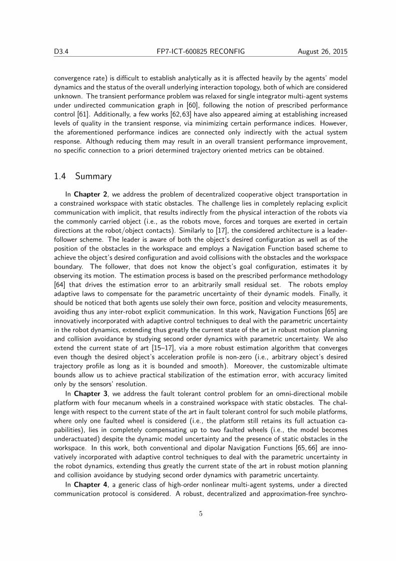
Figure 2.2: Two mobile manipulators handling a rigidly grasped object in a constrainedworkspace with static obstacles. Only the leader is aware of the object’s desired configurationand the obstacles’ position in the workspace.
2.3 Simulations
We consider a scenario involving oriented motion on a planar surface (i.e., the coordinates arex, y and the orientation ψ) with two mobile manipulators in a leader-follower scheme, handlinga rigidly grasped object in a constrained workspace with static obstacles (see Fig. 2.2). Theleader is aware of the obstacles’ position in the workspace and is assigned the desired object’sconfiguration, whereas the follower estimates it via the proposed algorithm (2.10), by simplyobserving the motion of the object and without communicating explicitly with the leader.
The workspace as well as the initial and the desired configuration of the object are depictedin Fig. 2.2. Apparently, the overall formation has to be aligned with the x-axis in order totransverse the obstacles. In this respect, we constructed a navigation function on the 3D space(i.e., x, y and ψ), adopting a virtual toroidal obstacle to model the aforementioned relation ofposition (x, y) with the orientation ψ. Moreover, the control gains were selected as follows: k = 2,kNF = 2, KL = 2.5I3×3, Λ = 1.5I3×3, KF = 2.5I3×3. Additionally, since the robots’ mass (i.e.,mL = mF = 2.5 kgr) was considered unknown, the adaptive laws (2.8) and (2.20) were adopted toprovide their estimates with control gains ΓL = 0.1 and ΓF = 0.15. Finally, the parameters of theproposed estimator were chosen as kj = 0.5, ρj(t) = (2 |ej (0)| + 0.1) e−3t + 0.05, j ∈ x, y, ψ.
16
D3.4 FP7-ICT-600825 RECONFIG August 26, 2015
−2.5
−2
−1.5
−1
−0.5
0
0.5
1
1.5
2
2.5
y
t = 0 sec
Leader
Follower
Object
t = 0.7 sec
Leader
Follower
Object
t = 2.5 sec
Leader
Follower
Object
−2 −1 0 1 2−2.5
−2
−1.5
−1
−0.5
0
0.5
1
1.5
2
2.5
x
y
t = 8.5 sec
Leader
Follower
Object
−2 −1 0 1 2x
t = 13 sec
Leader
Follower
Object
−2 −1 0 1 2x
t = 30 sec
Leader
Follower
Object
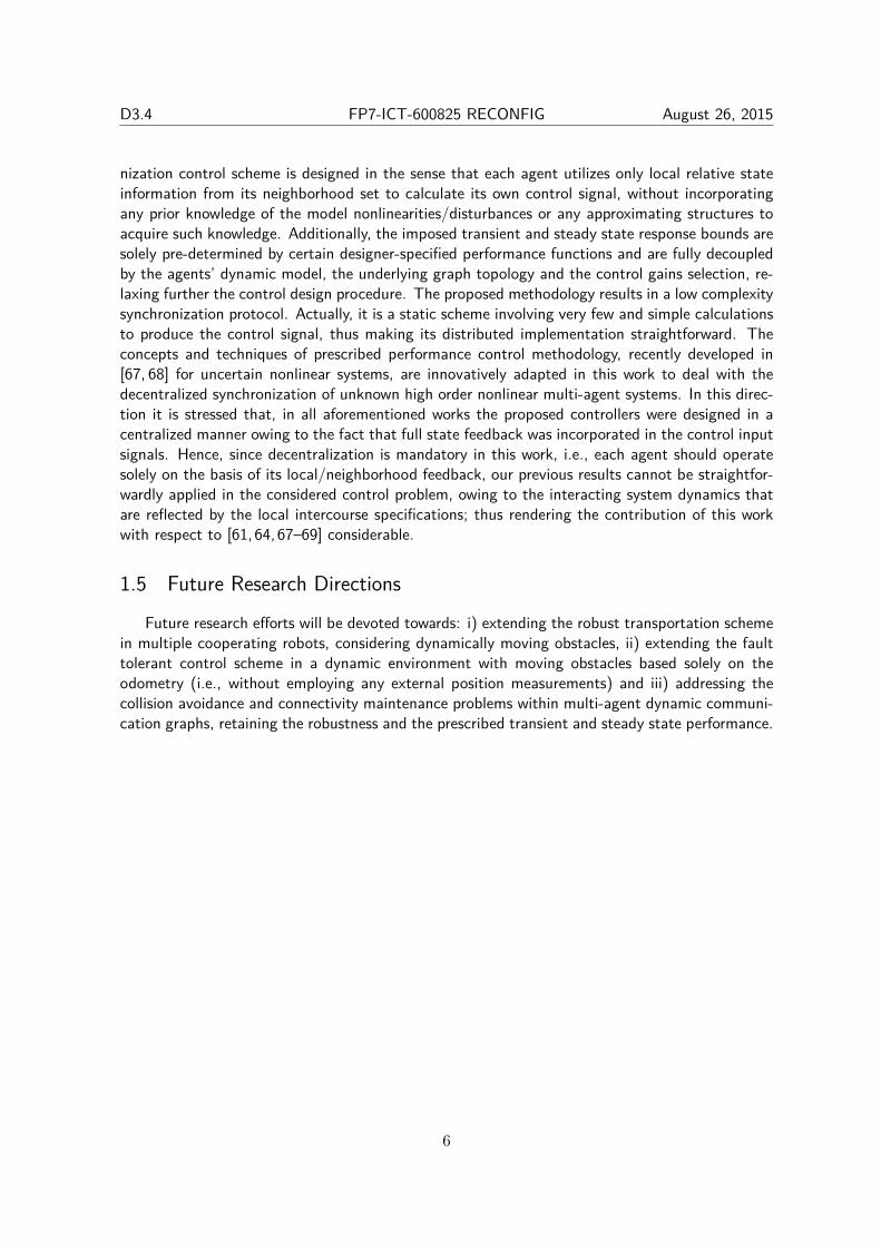
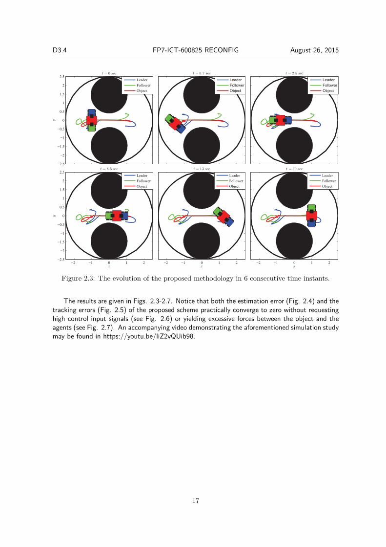
Figure 2.3: The evolution of the proposed methodology in 6 consecutive time instants.
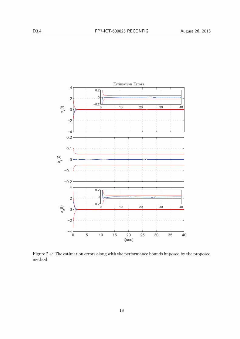
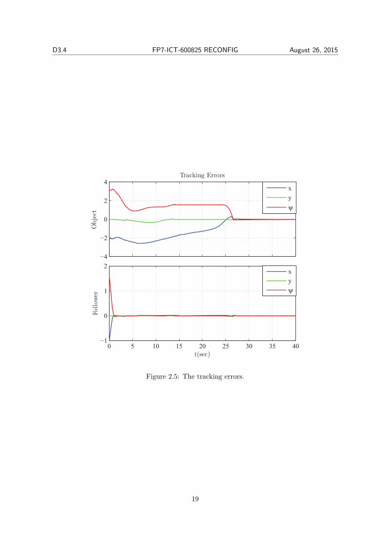
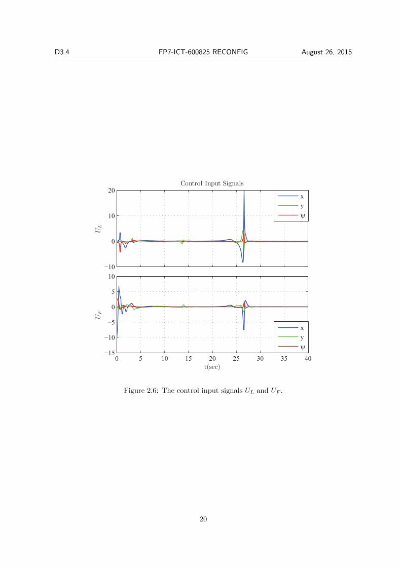
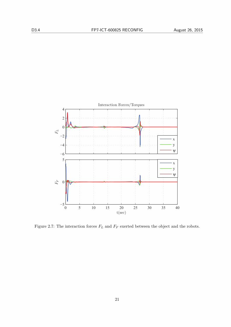
The results are given in Figs. 2.3-2.7. Notice that both the estimation error (Fig. 2.4) and thetracking errors (Fig. 2.5) of the proposed scheme practically converge to zero without requestinghigh control input signals (see Fig. 2.6) or yielding excessive forces between the object and theagents (see Fig. 2.7). An accompanying video demonstrating the aforementioned simulation studymay be found in https://youtu.be/liZ2vQUib98.
17
D3.4 FP7-ICT-600825 RECONFIG August 26, 2015
−4
−2
0
2
4
ex(t)
Estimation Errors
−0.2
−0.1
0
0.1
0.2
ey(t)
0 5 10 15 20 25 30 35 40−4
−2
0
2
4
t(sec)
eψ(t)
0 10 20 30 40−0.2
0
0.2
0 10 20 30 40−0.2
0
0.2
Figure 2.4: The estimation errors along with the performance bounds imposed by the proposedmethod.
18
D3.4 FP7-ICT-600825 RECONFIG August 26, 2015
−4
−2
0
2
4
Obje
ct
Tracking Errors
x
y
ψ
0 5 10 15 20 25 30 35 40−1
0
1
2
t(sec)
Follow
er
x
y
ψ
Figure 2.5: The tracking errors.
19
D3.4 FP7-ICT-600825 RECONFIG August 26, 2015
−10
0
10
20
UL
Control Input Signals
x
y
ψ
0 5 10 15 20 25 30 35 40−15
−10
−5
0
5
10
t(sec)
UF
x
y
ψ
Figure 2.6: The control input signals UL and UF .
20
D3.4 FP7-ICT-600825 RECONFIG August 26, 2015
−6
−4
−2
0
2
4
FL
Interaction Forces/Torques
x
y
ψ
0 5 10 15 20 25 30 35 40−5
0
5
t(sec)
FF
x
y
ψ
Figure 2.7: The interaction forces FL and FF exerted between the object and the robots.
21
Chapter 3
Fault Tolerant Control for Omni-directionalPlatforms
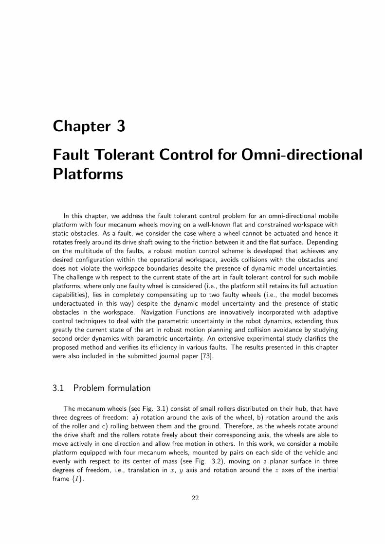
In this chapter, we address the fault tolerant control problem for an omni-directional mobileplatform with four mecanum wheels moving on a well-known flat and constrained workspace withstatic obstacles. As a fault, we consider the case where a wheel cannot be actuated and hence itrotates freely around its drive shaft owing to the friction between it and the flat surface. Dependingon the multitude of the faults, a robust motion control scheme is developed that achieves anydesired configuration within the operational workspace, avoids collisions with the obstacles anddoes not violate the workspace boundaries despite the presence of dynamic model uncertainties.The challenge with respect to the current state of the art in fault tolerant control for such mobileplatforms, where only one faulty wheel is considered (i.e., the platform still retains its full actuationcapabilities), lies in completely compensating up to two faulty wheels (i.e., the model becomesunderactuated in this way) despite the dynamic model uncertainty and the presence of staticobstacles in the workspace. Navigation Functions are innovatively incorporated with adaptivecontrol techniques to deal with the parametric uncertainty in the robot dynamics, extending thusgreatly the current state of the art in robust motion planning and collision avoidance by studyingsecond order dynamics with parametric uncertainty. An extensive experimental study clarifies theproposed method and verifies its efficiency in various faults. The results presented in this chapterwere also included in the submitted journal paper [73].
3.1 Problem formulation
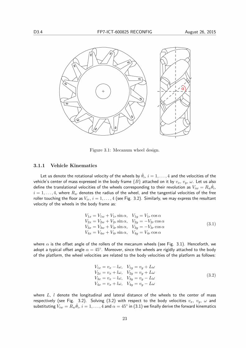
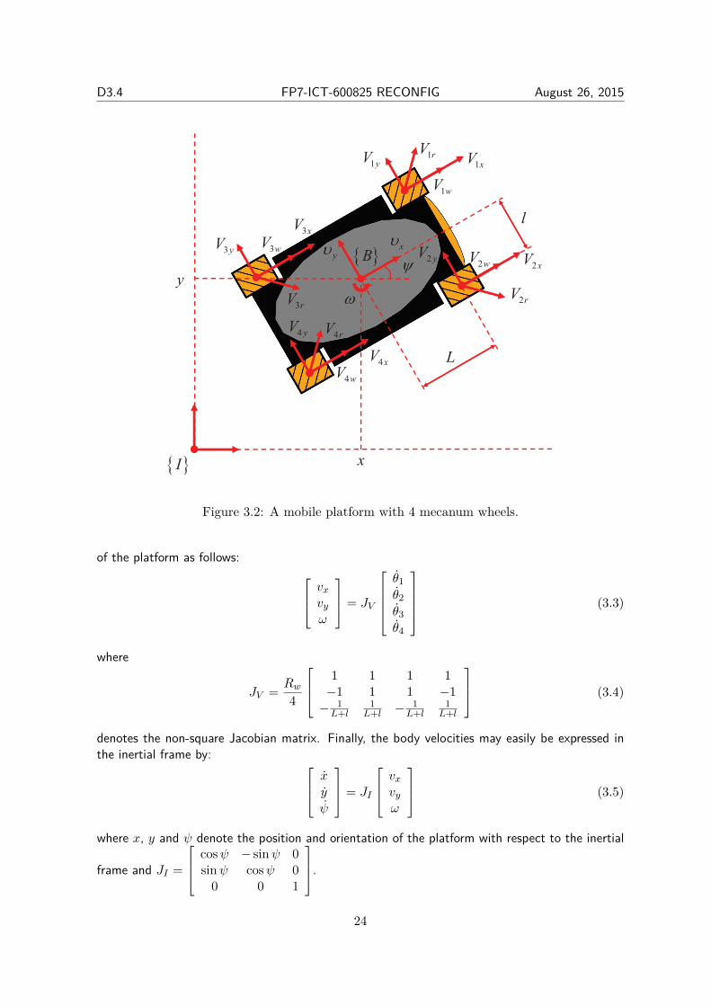
The mecanum wheels (see Fig. 3.1) consist of small rollers distributed on their hub, that havethree degrees of freedom: a) rotation around the axis of the wheel, b) rotation around the axisof the roller and c) rolling between them and the ground. Therefore, as the wheels rotate aroundthe drive shaft and the rollers rotate freely about their corresponding axis, the wheels are able tomove actively in one direction and allow free motion in others. In this work, we consider a mobileplatform equipped with four mecanum wheels, mounted by pairs on each side of the vehicle andevenly with respect to its center of mass (see Fig. 3.2), moving on a planar surface in threedegrees of freedom, i.e., translation in x, y axis and rotation around the z axes of the inertialframe I.
22
D3.4 FP7-ICT-600825 RECONFIG August 26, 2015
Figure 3.1: Mecanum wheel design.
3.1.1 Vehicle Kinematics
Let us denote the rotational velocity of the wheels by θi, i = 1, . . . , 4 and the velocities of thevehicle’s center of mass expressed in the body frame B attached on it by vx, vy, ω. Let us alsodefine the translational velocities of the wheels corresponding to their revolution as Viw = Rwθi,i = 1, . . . , 4, where Rw denotes the radius of the wheel, and the tangential velocities of the freeroller touching the floor as Vir, i = 1, . . . , 4 (see Fig. 3.2). Similarly, we may express the resultantvelocity of the wheels in the body frame as:
V1x = V1w + V1r sinα, V1y = V1r cosαV2x = V2w + V2r sinα, V2y = −V2r cosαV3x = V3w + V3r sinα, V3y = −V3r cosαV4x = V4w + V4r sinα, V4y = V4r cosα
(3.1)
where α is the offset angle of the rollers of the mecanum wheels (see Fig. 3.1). Henceforth, weadopt a typical offset angle α = 45. Moreover, since the wheels are rigidly attached to the bodyof the platform, the wheel velocities are related to the body velocities of the platform as follows:
V1x = vx − lω, V1y = vy + LωV2x = vx + lω, V2y = vy + LωV3x = vx − lω, V3y = vy − LωV4x = vx + lω, V4y = vy − Lω
(3.2)
where L, l denote the longitudinal and lateral distance of the wheels to the center of massrespectively (see Fig. 3.2). Solving (3.2) with respect to the body velocities vx, vy, ω andsubstituting Viw = Rwθi, i = 1, . . . , 4 and α = 45 in (3.1) we finally derive the forward kinematics
23
D3.4 FP7-ICT-600825 RECONFIG August 26, 2015
I
B
x
y
L
l
xy
1wV
3wV
2wV
4wV
1rV
2rV
4rV
3rV
3yV
4 yV
2 yV
1yV 1xV
2xV
4xV
3xV
Figure 3.2: A mobile platform with 4 mecanum wheels.
of the platform as follows: vx
vy
ω
= JV
θ1θ2θ3θ4
(3.3)
where
JV = Rw
4
1 1 1 1−1 1 1 −1
− 1L+l
1L+l − 1
L+l1
L+l
(3.4)
denotes the non-square Jacobian matrix. Finally, the body velocities may easily be expressed inthe inertial frame by: x
y
ψ
= JI
vx
vy
ω
(3.5)
where x, y and ψ denote the position and orientation of the platform with respect to the inertial
frame and JI =
cosψ − sinψ 0sinψ cosψ 0
0 0 1
.
24
D3.4 FP7-ICT-600825 RECONFIG August 26, 2015
3.1.2 Vehicle Dynamics
Since the vehicle moves on a planar surface its potential energy is kept constant. On theother hand, neglecting the inertia of the rollers, the kinetic energy of the platform is calculated asfollows:
K = 12m(x2 + y2
)+ 1
2Izψ
2 + 12Iw
(θ1 + θ2 + θ3 + θ4
)where m denotes the overall mass of the platform and Iz, Iw denote the moment of inertia of theplatform and the wheels respectively. Moreover, the loss of energy owing to the wheels’ viscousfriction is modeled as:
D = 12Dθ
(θ1 + θ2 + θ3 + θ4
)where Dθ denotes the friction coefficient. Finally, invoking the Lagrange equation, we obtain thevehicle’s dynamics:
Mθ +Dθθ = τ (3.6)
where θ = [θ1, θ2, θ3, θ4]T denotes the vector of the wheels’ angles, τ = [τ1, τ2, τ3, τ4]T is thevector of the applied wheel torques and
M =
A+B + Jw −B B A−B
−B A+B + Jw A−B BB A−B A+B + Jw −B
A−B B −B A+B + Jw
with A = mR2
w8 and B = JzR2
w16(L+l) .
3.1.3 Problem statement
Consider an omni-directional mobile platform with four mecanum wheels moving on a well-known flat and constrained workspace with static obstacles. We assume that measurements of itsposition, orientation and wheels’ velocities are available and that any slipping between the wheelsand the flat surface is negligible. Additionally, the geometric parameters (i.e., length, width andwheel radius) of the platform are considered known, whereas its dynamic parameters (i.e., massand moments of inertia) are completely unknown. The control objective is to design a robustcontrol scheme that achieves a desired configuration xd, yd, ψd within the operational workspace,avoids any collisions with the obstacles and does not violate the workspace boundaries despite thepresence of actuator (i.e., motor wheel) faults. As a faulty wheel, we consider the case where itcannot be actuated and hence it rotates freely around its drive shaft owing to the friction betweenit and the flat surface. In particular, we shall consider the nominal scenario where all wheels areoperating normally and owing to the kinematic redundancy of the platform four types of faults,namely one faulted wheel, two front or back wheels failure, two left or right side wheels failureand two diagonal wheels failure. Unfortunately, although when only one wheel is operating theposture of the platform may change theoretically, in practice this is not the case owing to the lowdriving force developed by one wheel. Hence, such case should be definitely considered as criticalsince no fault tolerance strategy can be developed. Finally, it should be noticed that owing to:i) the constrained workspace ii) the dynamic model uncertainties and iii) the fact that up to twofaulty wheels are compensated, the problem becomes very challenging, with no previously reportedresults in the related literature.
25
D3.4 FP7-ICT-600825 RECONFIG August 26, 2015
Remark 5. A fault tolerance control strategy is based on the development of a fault detectionsystem that systematically monitors possible abnormal events in the system. The inconsis-tencies between the actual and the expected behavior(called residuals), should be such thatfailures in the motor wheels can be detected and subsequently isolated by the control strategy.The residuals are calculated based on the position differences between the observer and theplant available by an external position sensor. However, since this work does not study howthese residuals are used to detect actuation faults, certain well-established fault detection algo-rithms [74, 75] may be adopted complementarily, without affecting the fault tolerance controlstrategy.
3.2 Fault Tolerant ControlThe control objective is to navigate the mobile platform towards the goal configuration while
avoiding collisions with the static obstacles that lie within the constrained workspace and despitethe presence of dynamic model uncertainties and up to two faulty wheels. Towards this direc-tion, the concept of Navigation Functions will be innovatively incorporated with adaptive controltechniques to deal with the parametric uncertainty in the robot dynamics (3.6), extending thusgreatly the current state of the art in fault tolerant control as well as in motion planning withcollision avoidance by studying second order dynamics with parametric uncertainty. Dependingon the multitude of the faulty wheels, appropriate motion control schemes will be designed for:i) the nominal case where all wheels are operating normally, ii) the case of one faulty wheel andfinally iii) the case of two wheels failure with various combinations.
3.2.1 No Faulty Wheels
The control design relies on the conventional Navigation Function originally proposed by Rimonand Koditschek in [65] as follows:
ΦNF (p, pd) = γ(p−pd)
(γk(p−pd)+β(p))1k
(3.7)
where p = [x, y, ψ]T denotes the overall state vector, k > 1 is a design constant, γ (p− pd) > 0with γ (0) = 0 represents the attractive potential field to the goal configuration pd = [xd, yd, ψd]Tand β (p) > 0 with lim
p→Boundary
Obstacles
β (p) = 0 represents the repulsive potential field by the workspace
boundary and the obstacle regions. Without loss of generality1, we adopt ellipsoidal regions tomodel the robots, the object, the workspace and the obstacles. In that respect, it was proven in[65] that ΦNF (p, pd) has a global minimum at pd and no other local minima for a sufficientlylarge k. Thus, a feasible path that leads from any initial obstacle-free configuration2 to the desiredconfiguration might be generated by following the negated gradient of ΦNF (p, pd). Consequently,the desired motion profile of the platform expressed in its body frame is designed as follows:
vd (t) = −kNFJTI ∇pΦNF (p (t) , pd) , kNF > 0. (3.8)
In the sequel, we propose an adaptive control scheme that guarantees the asymptotic stabilizationof the platform to the goal configuration pd.
1Other geometrically more complex workspaces may also be considered by adopting proper topologicallyequivalent transformations [71].
2Except from a set of measure zero [65].
26
D3.4 FP7-ICT-600825 RECONFIG August 26, 2015
Theorem 3. Consider the unknown mobile robot dynamics (3.6) and the desired motionprofile (3.8). The adaptive control scheme:
τ = M θd + Dθθd −KvS− 1
1−ΦNF (p,pd)JTV J
TI ∇pΦNF (p, pd) , Kv > 0
˙M = −ΓM θdS
T , ΓM > 0˙Dθ = −ΓDθdS
T , ΓD > 0
(3.9)
where θd (t) ≡ J+V vd (t) denotes the desired wheel velocity that yields from the desired motion
profile (3.8) via the inverse kinematics3 of (3.3), S (t) = θ (t)−θd (t) denotes the wheel velocityerror and M , Dθ denote the estimate of the unknown parameters of the dynamic model,guarantees for a sufficiently large parameter k > 1 of the Navigation Function ΦNF (p, pd)defined in (3.7), that the platform is asymptotically stabilized to pd, except from a set ofinitial conditions of measure zero.
Proof. Consider the positive definite function:
L = ln(
11−ΦNF (p,pd)
)+ 1
2STMS + 1
2trace(MT Γ−1
M M)
+ 12trace
(DT
θΓ−1
D Dθ
),
where M is the positive definite inertial matrix and M = M − M , Dθ = Dθ − Dθ de-note the parametric errors. Notice also that ΦNF (p, pd) takes values from the set [0, 1);hence the first term is well defined within the feasible workspace. Thus, differentiating Lwith respect to time, substituting the dynamics (3.6), adding and subtracting the terms
11−ΦNF (p,pd)∇T
p ΦNF (p, pd) JIvd, STDθθd and invoking the control scheme (3.9), we get:
L = − kNF1−ΦNF (p,pd) ∥∇pΦNF (p, pd)∥2 − STKvS ≤ 0.
Therefore, owing to the fact that 11−ΦNF (p,pd) > 1, we may conclude the boundedness of S,
M , Dθ, ln(
11−ΦNF (p,pd)
)and consequently p (t), θ (t) and vd (t). Hence, it can be easily de-
duced that ΦNF (p, pd) remains strictly less than 1, avoiding thus collisions with the obstaclesand the workspace boundary. Finally, employing LaSalle’s Invariant Principle, we can easilydeduce that limt→∞ ∥∇pΦNF (p (t) , pd)∥ = 0 and limt→∞
∥∥∥θ (t)∥∥∥ = 0. However, although
∥∇pΦNF (p, pd)∥ = 0 occurs at either the goal configuration pd or at a saddle point, for suffi-ciently large k > 1 all saddle points of ΦNF (p, pd) are isolated [65] and hence, the set of initialconditions that lead to them are sets of measure zero [72]. As a result, the proposed controlscheme guarantees the asymptotic stabilization of the platform to the desired configurationpd, except from a set of initial conditions of measure zero, which completes the proof.
Remark 6. Navigation Functions and generic Artificial Potential Fields have been exten-sively employed in the past to tackle with the robot navigation problem. However, only simpledynamics (i.e., single and double integrators) have be considered so far without studying any
3In this work we adopt the Moore-Penrose pseudo-inverse J+V ≡
(JT
V JV
)−1JT
V , which provides the minimumnorm solution to the inverse kinematics problem.
27
D3.4 FP7-ICT-600825 RECONFIG August 26, 2015
robustness issues against uncertainties in nonlinear models. In this work, Navigation Func-tions are innovatively incorporated with adaptive control techniques to deal with parametricuncertainty in the robot dynamics, extending thus greatly the current state of the art in motionplanning and collision avoidance.
3.2.2 One Faulty Wheel
Owing to their kinematic redundancy, omni-directional mobile platforms equipped with fourmecanum wheels can still operate efficiently with three wheels, in case some malfunctioning inone wheel has been detected. In this respect, we may apply identical arguments with the nominalcase, as presented previously. Hence, the desired wheel velocity is calculated by the desired motionprofile (3.8) via θd (t) ≡ J−1
V vd (t), where JV yields from JV by simply neglecting the columnthat corresponds to the faulty wheel. In the same way, the corresponding blocks of the unknownmatrices M , Dθ are estimated by similar adaptive laws in (3.9). Fortunately, the motion of thefaulty wheel, produced by the friction of the wheel with the flat surface, appears as a vanishingdisturbance in the dynamic model and does not affect the stability of the closed loop system owingto its input to state stability property (i.e., the matrix Dθ is positive definite).
3.2.3 Two Faulty Wheels
When the motion is produced by only two driving wheels, then the platform becomes inevitablyunderactuated, since it cannot move in both directions and rotate independently on the flat surface(i.e., unicycle-like motion). Fortunately, in such cases dipolar navigation functions [66] have beenproven a very effective stabilizing tool, owing to their key advantage to drive an underactuatedunicycle-like mobile robot to its destination with the desired orientation. Such property derivesnaturally from the fact that the flows of the corresponding vector fields are tangent to the desiredorientation ψd at the destination point pd = [xd, yd]T .
Depending on the combinations of the faulty wheels, appropriate state transformations [X,Y,Ψ]T =T (x, y, ψ) can be adopted to convert the kinematics of the mobile platform (3.3)-(3.5) into aunicycle-like model. Subsequently, a dipolar navigation function is constructed and incorporatedwith the adaptive backstepping technique to deal with the dynamic model uncertainties.
Front Wheels
In case the front wheels are faulty (i.e., wheels 1 and 2 are malfunctioning), the followingtransformation: X
YΨ
=
xyψ
+
cosψsinψ
0
(L+ l)
that shifts the centre of rotation L+ l forward, leads to a unicycle-like model:[X
Y
]=[
cos Ψsin Ψ
]U(θ3, θ4
)+ ∆X,Y
(θ1, θ2
)Ψ = R
(θ3, θ4
)+ ∆Ψ
(θ1, θ2
)where U
(θ3, θ4
)= Rw
4
(θ3 + θ4
)and R
(θ3, θ4
)= Rw
4(L+l)
(−θ3 + θ4
)act as the longitudinal
and rotational velocity with respect to the new centre of rotation and ∆X,Y
(θ1, θ2
), ∆Ψ
(θ1, θ2
)28
D3.4 FP7-ICT-600825 RECONFIG August 26, 2015
denote residual terms owing to the motion of the faulty wheels, produced by the friction of thewheels with the flat surface. Finally, notice that U
(θ3, θ4
), R
(θ3, θ4
)can be easily solved with
respect to θ3, θ4, thus providing us with a nonsingular mapping between body velocities and wheelvelocities.
Back Wheels
In case the back wheels are faulty (i.e., wheels 3 and 4 are malfunctioning), the followingtransformation: X
YΨ
=
xyψ
−
cosψsinψ
0
(L+ l)
that shifts the centre of rotation L+ l backwards, leads to a unicycle-like model:[X
Y
]=[
cos Ψsin Ψ
]U(θ1, θ2
)+ ∆X,Y
(θ3, θ4
)Ψ = R
(θ1, θ2
)+ ∆Ψ
(θ3, θ4
)where U
(θ1, θ2
)= Rw
4
(θ1 + θ2
)and R
(θ1, θ2
)= Rw
4(L+l)
(−θ1 + θ2
)act as the longitudinal
and rotational velocity with respect to the new centre of rotation and ∆X,Y
(θ1, θ2
), ∆Ψ
(θ1, θ2
)denote residual terms owing to the motion of the faulty wheels, produced by the friction of thewheels with the flat surface.
Left Wheels
In case the left wheels are faulty (i.e., wheels 1 and 3 are malfunctioning), the followingtransformation: X
YΨ
=
xy
ψ + π2
+
cos(ψ + π
2)
sin(ψ + π
2)
0
(L+ l)
that shifts the centre of rotation L + l to the left and rotates it π2 anti-clockwise, leads to a
unicycle-like model: [X
Y
]=[
cos Ψsin Ψ
]U(θ2, θ4
)+ ∆X,Y
(θ1, θ3
)Ψ = R
(θ2, θ4
)+ ∆Ψ
(θ1, θ3
)where U
(θ2, θ4
)= Rw
4
(θ2 − θ4
)and R
(θ2, θ4
)= Rw
4(L+l)
(θ2 + θ4
)act as the longitudinal and
rotational velocity with respect to the new centre of rotation and ∆X,Y
(θ1, θ3
), ∆Ψ
(θ1, θ3
)denote residual terms owing to the motion of the faulty wheels, produced by the friction of thewheels with the flat surface.
29
D3.4 FP7-ICT-600825 RECONFIG August 26, 2015
Right Wheels
In case the right wheels are faulty (i.e., wheels 2 and 4 are malfunctioning), the followingtransformation: X
YΨ
=
xy
ψ − π2
+
cos(ψ − π
2)
sin(ψ − π
2)
0
(L+ l)
that shifts the centre of rotation L+l to the right and rotates it π2 clockwise, leads to a unicycle-like
model: [X
Y
]=[
cos Ψsin Ψ
]U(θ1, θ3
)+ ∆X,Y
(θ2, θ4
)Ψ = R
(θ1, θ3
)+ ∆Ψ
(θ2, θ4
)where U
(θ1, θ3
)= Rw
4
(θ1 − θ3
)and R
(θ1, θ3
)= Rw
4(L+l)
(−θ1 − θ3
)act as the longitudinal
and rotational velocity with respect to the new centre of rotation and ∆X,Y
(θ2, θ4
), ∆Ψ
(θ2, θ4
)denote residual terms owing to the motion of the faulty wheels, produced by the friction of thewheels with the flat surface.
Main Diagonal Wheels
In case the wheels in the main diagonal are faulty (i.e., wheels 1 and 4 are malfunctioning),the following transformation: X
YΨ
=
xy
ψ + π4
that rotates the centre of rotation π
4 anti-clockwise, leads to a unicycle-like model:[X
Y
]=[
cos Ψsin Ψ
]U(θ2, θ3
)+ ∆X,Y
(θ1, θ4
)Ψ = R
(θ2, θ3
)+ ∆Ψ
(θ1, θ4
)where U
(θ2, θ3
)= Rw
√2
4
(θ2 + θ3
)and R
(θ2, θ3
)= Rw
4(L+l)
(θ2 − θ3
)act as the longitudinal
and rotational velocity with respect to the new centre of rotation and ∆X,Y
(θ1, θ4
), ∆Ψ
(θ1, θ4
)denote residual terms owing to the motion of the faulty wheels, produced by the friction of thewheels with the flat surface.
Secondary Diagonal Wheels
In case the wheels in the secondary diagonal are faulty (i.e., wheels 2 and 3 are malfunctioning),the following transformation: X
YΨ
=
xy
ψ − π4
30
D3.4 FP7-ICT-600825 RECONFIG August 26, 2015
that rotates the centre of rotation π4 clockwise, leads to a unicycle-like model:[
X
Y
]=[
cos Ψsin Ψ
]U(θ1, θ4
)+ ∆X,Y
(θ2, θ3
)Ψ = R
(θ1, θ4
)+ ∆Ψ
(θ2, θ3
)where U
(θ1, θ4
)= Rw
√2
4
(θ1 + θ4
)and R
(θ1, θ4
)= Rw
4(L+l)
(−θ1 + θ4
)act as the longitudinal
and rotational velocity with respect to the new centre of rotation and ∆X,Y
(θ2, θ3
), ∆Ψ
(θ2, θ3
)denote residual terms owing to the motion of the faulty wheels, produced by the friction of thewheels with the flat surface.
Control Scheme
To be able to produce a dipolar vector field, the conventional navigation function (3.7) ismodified as follows:
ΦDNF (P, Pd,Ψd) = γ(P −Pd)
(γk(P −Pd)+H(P,Pd,Ψd)β(P ))1k
where P = [X,Y ]T and Pd = [Xd, Yd]T denote the transformed position and destination of theplatform, Ψd denotes the transformed desired orientation at the destination, H (P, Pd,Ψd) = ε+|[cos Ψd, sin Ψd] (P − Pd)|2 represents a pseudo-obstacle that enforces the dipolar property of thevector field and ε > 0 is a scalar positive parameter that ensures the aforementioned modificationdoes not affect the navigation properties presented in Subsection 3.2.1 [76]. Consequently, thedesired motion profile of the platform expressed in its body frame is designed as follows:
Ud (t) = −kNFS(∥∇pΦDNF ∥2 + ∥P − Pd∥2
)Rd (t) = −kNF (Ψ − Ψ⋆) + Ψ⋆, kNF > 0.
where S = sgn(
∂ΦDNF∂X cos Ψ + ∂ΦDNF
∂Y sin Ψ)
and Ψ⋆ = arctan(
∂ΦDNF∂Y /∂ΦDNF
∂X
)denotes the
orientation of the flows of the dipolar vector field. Notice that the aforementioned motion profileaims at aligning the platform with the flows of the dipolar vector field and heading it towards thedestination, where the field is tangent to the desired orientation. Additionally, we may calculatethe desired velocity of the driving wheels as mentioned previously. Hence following identicalarguments with the nominal case, the corresponding blocks of the unknown matrices M , Dθ mayalso be estimated by similar adaptive laws to (3.9). Fortunately, the motion of the faulty wheels,produced by the friction of the wheels with the flat surface, appears as a vanishing disturbance inthe dynamic model and does not affect the stability of the closed loop system owing to its inputto state stability property (i.e., the matrix Dθ is positive definite).
3.3 Experimental ResultsThe experimental setup involves a KUKA youBot omni-directional mobile platform, which
is equipped with 4 mecanum wheels mounted by pairs at each side of the vehicle, evenly withrespect to its center of mass. A vision system consisting of a PS3 calibrated camera is also usedto calculate the position and orientation of the platform. The camera is mounted on the ceiling,
31
D3.4 FP7-ICT-600825 RECONFIG August 26, 2015
−1.5 −1 −0.5 0 0.5 1 1.5
−1
−0.5
0
0.5
1
x [m]
y [
m]
Faulted Wheels:
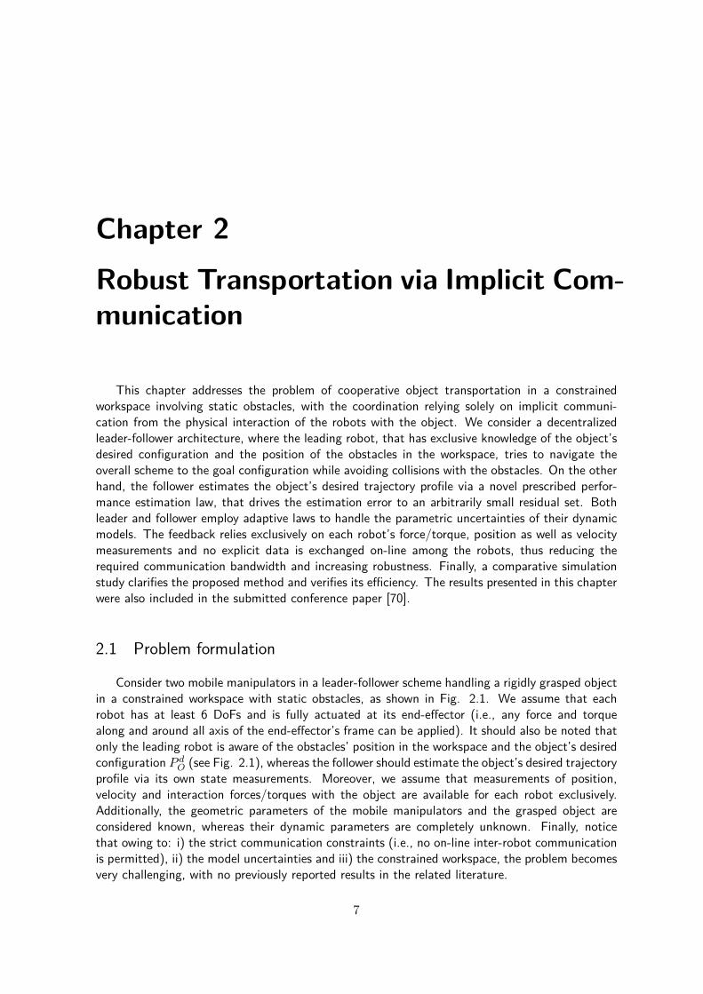
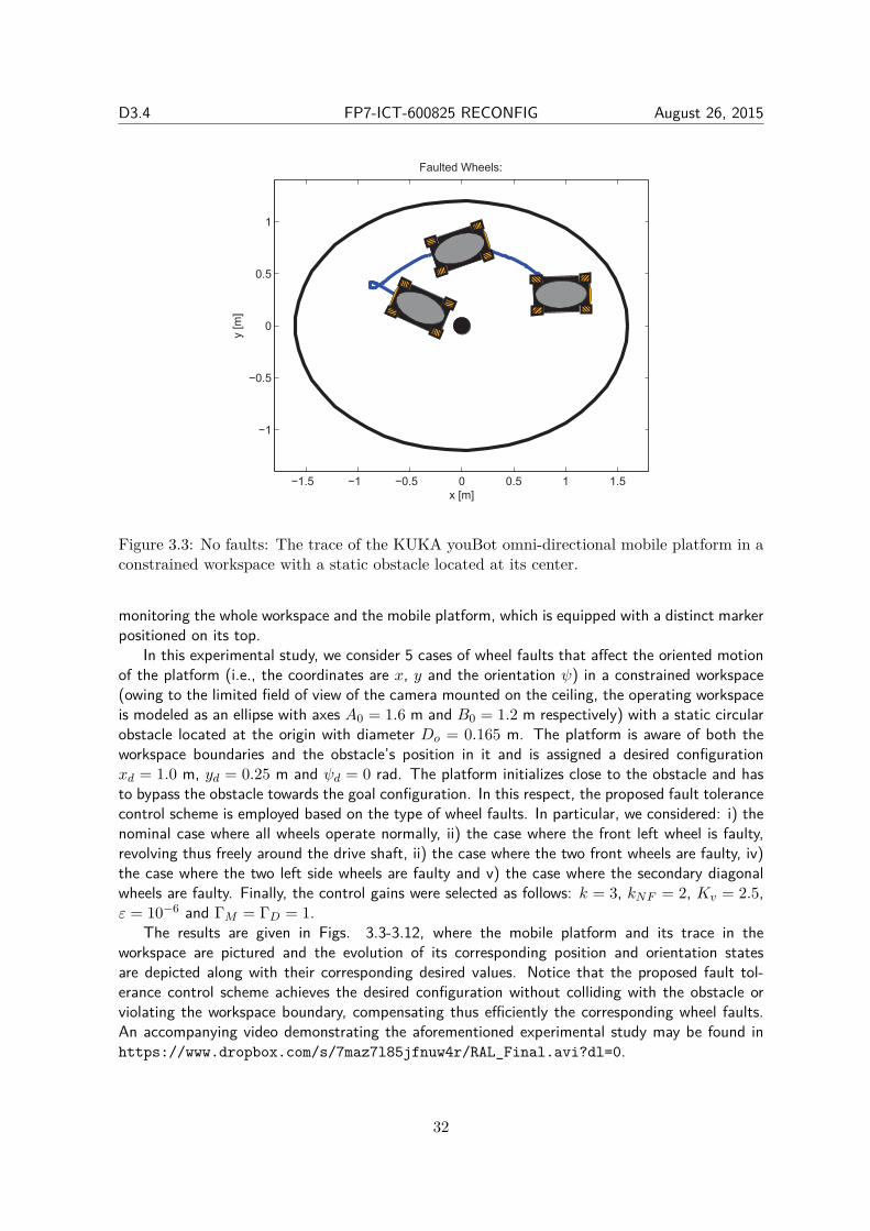
Figure 3.3: No faults: The trace of the KUKA youBot omni-directional mobile platform in aconstrained workspace with a static obstacle located at its center.
monitoring the whole workspace and the mobile platform, which is equipped with a distinct markerpositioned on its top.
In this experimental study, we consider 5 cases of wheel faults that affect the oriented motionof the platform (i.e., the coordinates are x, y and the orientation ψ) in a constrained workspace(owing to the limited field of view of the camera mounted on the ceiling, the operating workspaceis modeled as an ellipse with axes A0 = 1.6 m and B0 = 1.2 m respectively) with a static circularobstacle located at the origin with diameter Do = 0.165 m. The platform is aware of both theworkspace boundaries and the obstacle’s position in it and is assigned a desired configurationxd = 1.0 m, yd = 0.25 m and ψd = 0 rad. The platform initializes close to the obstacle and hasto bypass the obstacle towards the goal configuration. In this respect, the proposed fault tolerancecontrol scheme is employed based on the type of wheel faults. In particular, we considered: i) thenominal case where all wheels operate normally, ii) the case where the front left wheel is faulty,revolving thus freely around the drive shaft, ii) the case where the two front wheels are faulty, iv)the case where the two left side wheels are faulty and v) the case where the secondary diagonalwheels are faulty. Finally, the control gains were selected as follows: k = 3, kNF = 2, Kv = 2.5,ε = 10−6 and ΓM = ΓD = 1.
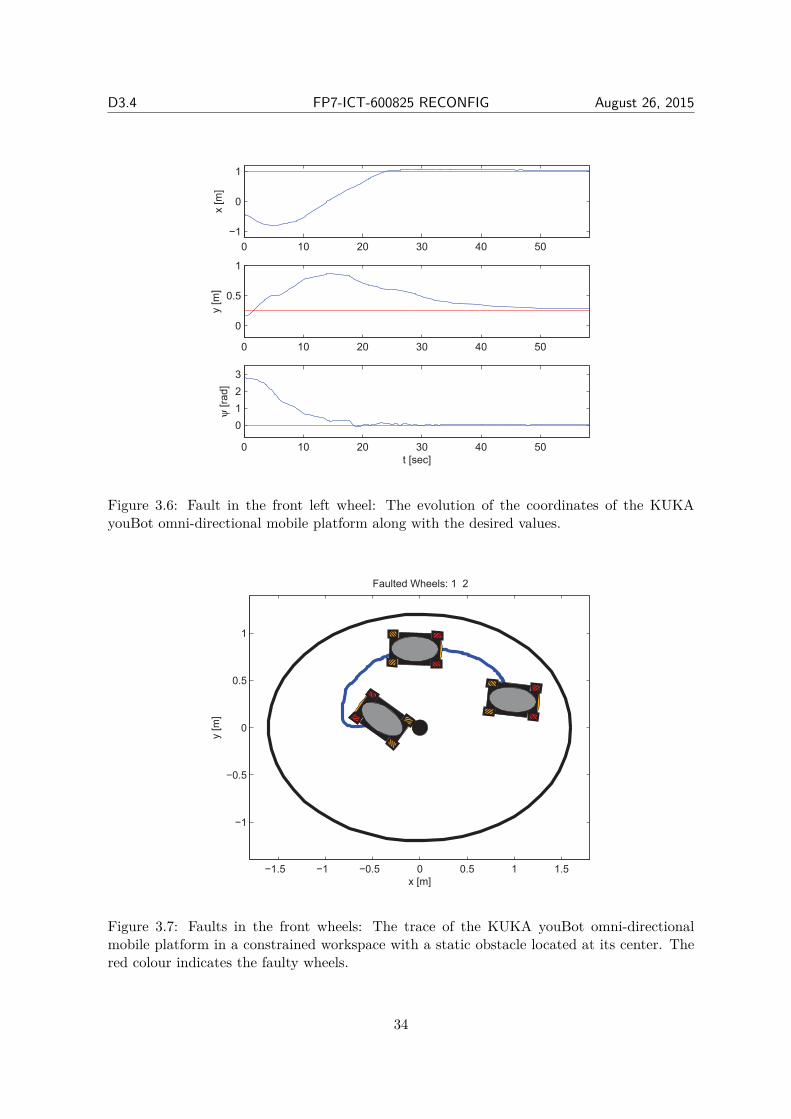
The results are given in Figs. 3.3-3.12, where the mobile platform and its trace in theworkspace are pictured and the evolution of its corresponding position and orientation statesare depicted along with their corresponding desired values. Notice that the proposed fault tol-erance control scheme achieves the desired configuration without colliding with the obstacle orviolating the workspace boundary, compensating thus efficiently the corresponding wheel faults.An accompanying video demonstrating the aforementioned experimental study may be found inhttps://www.dropbox.com/s/7maz7l85jfnuw4r/RAL_Final.avi?dl=0.
32
D3.4 FP7-ICT-600825 RECONFIG August 26, 2015
0 5 10 15 20 25 30 35 40 45
−1
0
1
x [
m]
0 5 10 15 20 25 30 35 40 45
0
0.5
1
y [
m]
0 5 10 15 20 25 30 35 40 45
0
1
2
3
ψ [
rad]
t [sec]
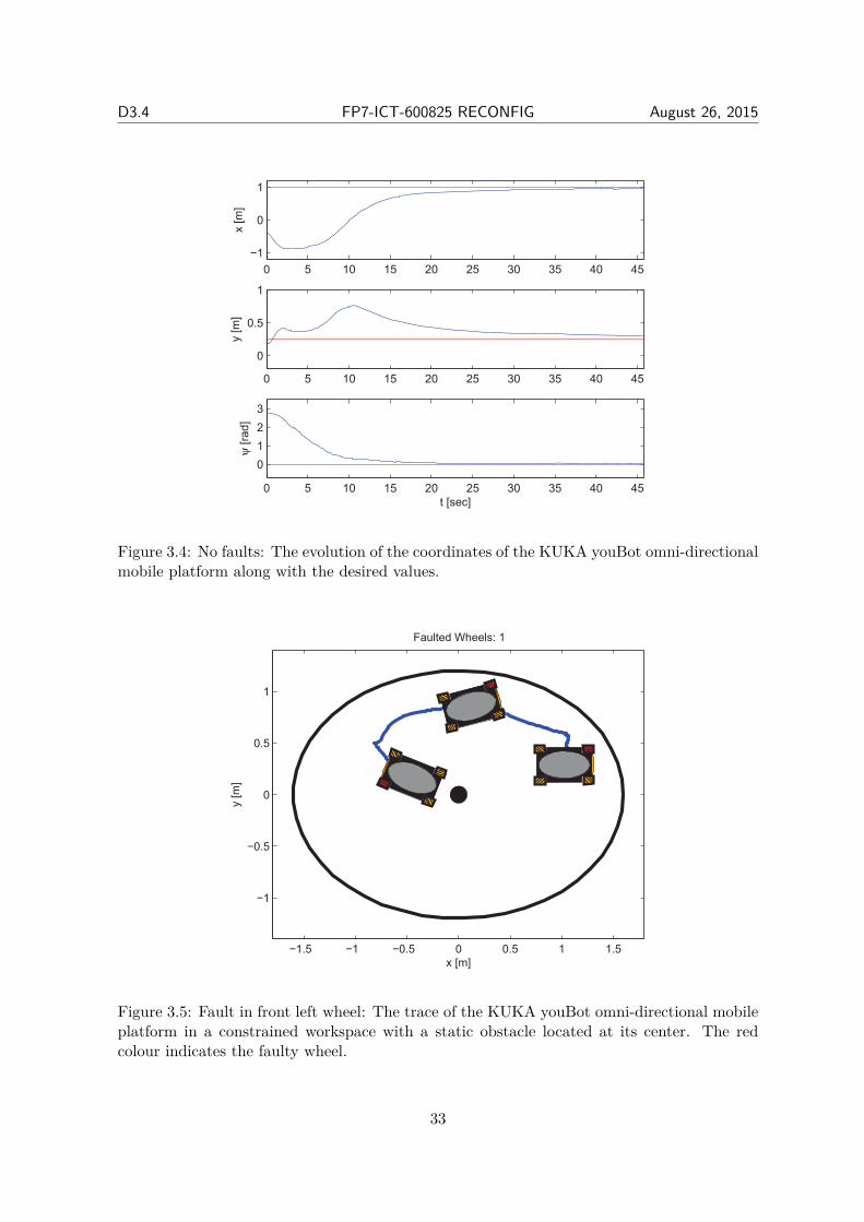
Figure 3.4: No faults: The evolution of the coordinates of the KUKA youBot omni-directionalmobile platform along with the desired values.
−1.5 −1 −0.5 0 0.5 1 1.5
−1
−0.5
0
0.5
1
x [m]
y [
m]
Faulted Wheels: 1
Figure 3.5: Fault in front left wheel: The trace of the KUKA youBot omni-directional mobileplatform in a constrained workspace with a static obstacle located at its center. The redcolour indicates the faulty wheel.
33
D3.4 FP7-ICT-600825 RECONFIG August 26, 2015
0 10 20 30 40 50
−1
0
1
x [
m]
0 10 20 30 40 50
0
0.5
1
y [
m]
0 10 20 30 40 50
0
1
2
3
ψ [
rad]
t [sec]
Figure 3.6: Fault in the front left wheel: The evolution of the coordinates of the KUKAyouBot omni-directional mobile platform along with the desired values.
−1.5 −1 −0.5 0 0.5 1 1.5
−1
−0.5
0
0.5
1
x [m]
y [
m]
Faulted Wheels: 1 2
Figure 3.7: Faults in the front wheels: The trace of the KUKA youBot omni-directionalmobile platform in a constrained workspace with a static obstacle located at its center. Thered colour indicates the faulty wheels.
34
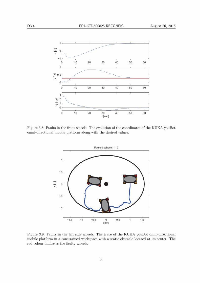
D3.4 FP7-ICT-600825 RECONFIG August 26, 2015
0 10 20 30 40 50 60
−1
0
1
x [
m]
0 10 20 30 40 50 60
0
0.5
1
y [
m]
0 10 20 30 40 50 60
0
1
2
3
ψ [
rad]
t [sec]
Figure 3.8: Faults in the front wheels: The evolution of the coordinates of the KUKA youBotomni-directional mobile platform along with the desired values.
−1.5 −1 −0.5 0 0.5 1 1.5
−1
−0.5
0
0.5
1
x [m]
y [
m]
Faulted Wheels: 1 3
Figure 3.9: Faults in the left side wheels: The trace of the KUKA youBot omni-directionalmobile platform in a constrained workspace with a static obstacle located at its center. Thered colour indicates the faulty wheels.
35
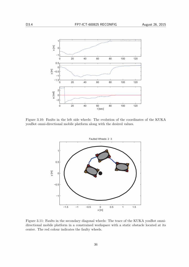
D3.4 FP7-ICT-600825 RECONFIG August 26, 2015
0 20 40 60 80 100 120
−1
0
1
x [
m]
0 20 40 60 80 100 120−1.5
−1
−0.5
0
0.5
y [
m]
0 20 40 60 80 100 120
−2
0
2
ψ [
rad]
t [sec]
Figure 3.10: Faults in the left side wheels: The evolution of the coordinates of the KUKAyouBot omni-directional mobile platform along with the desired values.
−1.5 −1 −0.5 0 0.5 1 1.5
−1
−0.5
0
0.5
1
x [m]
y [
m]
Faulted Wheels: 2 3
Figure 3.11: Faults in the secondary diagonal wheels: The trace of the KUKA youBot omni-directional mobile platform in a constrained workspace with a static obstacle located at itscenter. The red colour indicates the faulty wheels.
36
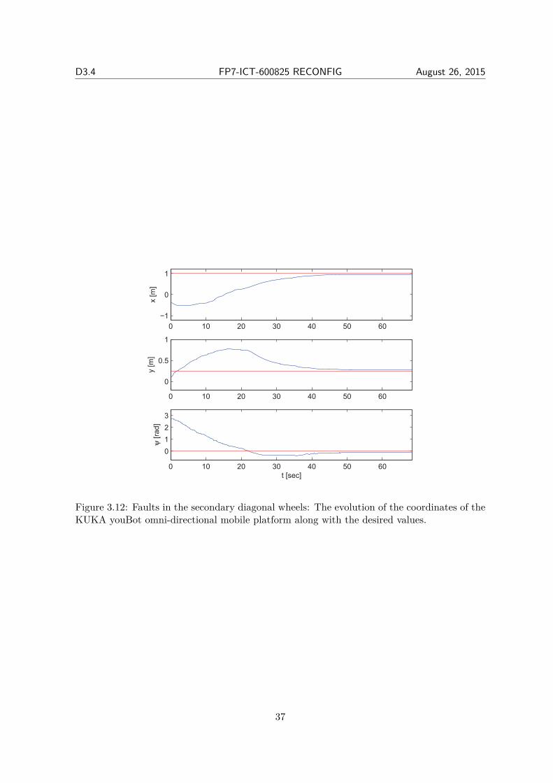
D3.4 FP7-ICT-600825 RECONFIG August 26, 2015
0 10 20 30 40 50 60
−1
0
1
x [
m]
0 10 20 30 40 50 60
0
0.5
1
y [
m]
0 10 20 30 40 50 60
0
1
2
3
ψ [
rad]
t [sec]
Figure 3.12: Faults in the secondary diagonal wheels: The evolution of the coordinates of theKUKA youBot omni-directional mobile platform along with the desired values.
37
Chapter 4Robust Cooperation for Multi-Agent Sys-tems
In this chapter, we consider the cooperative control problem for uncertain high-order nonlin-ear multi-agent systems in a leader-follower scheme, under a directed communication protocol.A robust decentralized control law of minimal complexity is proposed that achieves prescribed,arbitrarily fast and accurate synchronization of the following agents with the leader. The controlprotocol is purely decentralized in the sense that the control signal of each agent is calculatedbased solely on local relative state information from its neighborhood set. Additionally, no in-formation regarding the agents’ dynamic model is employed in the design procedure. Moreover,provided that the communication graph is connected and contrary to the related works on multi-agent systems, the controller-imposed transient and steady state performance bounds are fullydecoupled from the underlying graph topology, the control gains selection and the agents’ modeluncertainties, and are solely prescribed by certain designer-specified performance functions. Ex-tensive simulation results clarify and verify the approach. The results presented in this chapterwere also included in the journal paper [77] that was accepted for publication.
4.1 Problem Formulation and Preliminaries
Consider a multi-agent group comprised of a leader and N followers, with the leading agentacting as an exosystem that generates a desired command/reference trajectory for the multi-agentgroup. The followers, which have to be controlled, obey an m-th order nonlinear dynamic modelin canonical form, described as follows:
xi,j = xi,j+1, j = 1, . . . ,m− 1xi,m = fi (xi) + giui + di (t)
, i = 1, . . . , N (4.1)
where xi = [xi,1, . . . , xi,m]T ∈ ℜm, i = 1, . . . , N denote the state vector of each agent, fi, :ℜm → ℜ, i = 1, . . . , N are unknown locally Lipschitz functions, gi ∈ ℜ, i = 1, . . . , N areunknown constant parameters, ui ∈ ℜ, i = 1, . . . , N are the control inputs and di : ℜ+ → ℜ,i = 1, . . . , N represent piecewise continuous and bounded external disturbance terms. Apartfrom a sufficient controllability condition, i.e., the parameters gi, i = 1, . . . , N are consideredeither strictly positive or strictly negative, no further assumption is made on the stability of theaforementioned open loop nonlinear dynamics. Moreover, with no loss of generality, it is assumed
38
D3.4 FP7-ICT-600825 RECONFIG August 26, 2015
that gi > 0, i = 1, . . . , N . Additionally, defining the j-th order state vector of the multi-agentsystem as xj = [x1,j , . . . , xN,j ]T ∈ ℜN , the multi-agent dynamic model in vector form is writtenas follows:
˙xj = xj+1, j = 1, . . . ,m− 1˙xm = F (x) +Gu+ d (t) (4.2)
where x =[xT
1 , . . . , xTm
]T∈ ℜmN is the overall state vector with F (x) = [f1 (x1) , . . . , fN (xN )]T ,
G = diag ([g1, . . . , gN ]), u = [u1, . . . , uN ]T and d (t) = [d1 (t) , . . . , dN (t)]T . Furthermore, thestate/command variables of the leading agent are given by x0 (t) :=
[x0 (t) , x0 (t) , . . . , x(m−1)
0 (t)]T
∈ ℜm, where x0 : ℜ+ → ℜ and its derivatives up to m-th order are assumed to be continuousand bounded.
A directed graph (digraph) G = (V, E) is used to model the communication among the agents,where V = v1, . . . , vN denotes the set of vertices that represent the agents and E ⊆ V × Vdenotes the set of edges. The graph is assumed to be simple, i.e., (vi, vi) /∈ E (there exist no selfloops). The adjacency matrix associated with the digraph G is denoted as A = [aij ] ∈ ℜN×N
with aij ∈ 0, 1, i, j = 1, . . . , N . If aij = 1 then the agent i obtains information regarding thestate of the j-th agent (i.e., (vi, vj) ∈ E), whereas if aij = 0 then there is no state-informationflow from agent j to agent i (i.e., (vi, vj) /∈ E). The set of neighbors of a vertex vi is denotedby Ni = vj : (vi, vj) ∈ E and the degree matrix is defined as D = diag ([Di]) ∈ ℜN×N withDi =
∑j∈Ni
aij . In this respect, the graph Laplacian matrix is denoted by L = D − A ∈ℜN×N . The state information of the leader node (labeled v0) is only provided to a subgroupof the N agents. The access of the following agents to the leader’s state is modeled by adiagonal matrix B = diag ([b1, b2 . . . , bn]) ∈ ℜN×N . If bi, i ∈ 1, 2, . . . , N is equal to 1, thenthe i-th agent obtains state-information from the leader node; otherwise bi, i ∈ 1, 2, . . . , Nequals to 0. The augmented graph is defined as G =
(V, E
), where V = v0, v1, . . . , vN and
E= E ∪ (vi, v0) : bi = 1 ⊆ V × V while Ni =vj : (vi, vj) ∈ E
, i = 1, . . . , N denotes the
augmented set of neighbors.In the sequel, the robust synchronization control problem with prescribed performance to be
confronted in this work is formulated for the multi-agent system (4.2). More specifically, thetarget is to design a distributed control protocol, of low computational complexity for all thefollowing agents, considering relative state feedback, unknown model nonlinearities and externaldisturbances, such that the j-th order disagreement error vectors:
δj (t) = xj (t) − x0,j (t) ∈ ℜN , j = 1, . . . ,m (4.3)
with x0,j (t) :=[x
(j−1)0 (t) , . . . , x(j−1)
0 (t)]T
∈ ℜN , j = 1, . . . ,m are driven with predefinedminimum convergence rate within prespecified and arbitrarily small neighborhoods of the origin,keeping all closed loop signals bounded.Remark 7. Alternatively, a formation control problem, in which the multi-agent group shouldcreate arbitrarily fast and maintain with arbitrary accuracy a constant feasible (in the sense of[78]) formation, described by the desired relative offsets cij, i = 1, . . . , N with respect to eachmember j ∈ 0, 1, . . . , N of their augmented communication set Ni, could also be considered.
To solve the aforementioned multi-agent control problem, the following assumption regardingthe underlying communication graph topology is required.Assumption A1: The augmented graph G contains a spanning tree with the root being the leadernode.
39
D3.4 FP7-ICT-600825 RECONFIG August 26, 2015
Remark 8. The following common graph topologies satisfy Assumption A1:
1. The graph G contains a spanning tree and at least the root node can get access to theleader node.
2. The communication graph G is strongly connected and there exists at least one bi = 0,i ∈ 1, 2, . . . , N for all t ≥ 0.
3. The augmented graph G has an hierarchical structure1[79].
In addition, Assumption A1 dictates that L+B is a nonsingular M-matrix2[80].
Finally, the following technical lemma regarding nonsingular M-matrices will be employed toderive the main results of this work.
Lemma 2. ([81] in pp.168) Consider a nonsingular M-matrix W ∈ ℜN×N . There exists adiagonal positive definite matrix P = (diag (q))−1, with q = W−11 and 1 := [1, . . . , 1]T ∈ ℜN ,such that PW +W TP is also positive definite.
4.2 Main Results
4.2.1 Sufficient Conditions
Owing to considering distributed control protocols with relative state information, the controllaw of each agent i ∈ 1, . . . , N will be based on its neighborhood error feedback:
ei,j =∑l∈Ni
ail (xi,j − xl,j) + bi
(xi,j − x
(j−1)0
), j = 1, . . . ,m. (4.4)
Let us also define the j-th order neighborhood error vectors as ej = [e1,j , . . . , eN,j ]T , j = 1, . . . ,mwhich, employing the graph topology and after some trivial algebraic manipulations, become:
ej = (L+B) δj , j = 1, . . . ,m (4.5)
where the disagreement error vectors δj (t), j = 1, . . . ,m are defined in (4.3). Apparently, thej-th order neighborhood errors ej , j = 1, . . . ,m are expressed with respect to the leader state viathe corresponding j-th order disagreement error variables δj , j = 1, . . . ,m, which according tothe problem statement are required to enter arbitrarily fast into arbitrarily small neighborhoods ofthe origin. However, the disagreement variables δj , j = 1, . . . , N are global quantities and thuscannot be measured distributively based on the local intercourse specifications, as they involveinformation directly from the leader. Nevertheless, utilizing the nonsingularity of L+B, owing toAssumption A1, (4.5) yields: ∥∥∥δj
∥∥∥ ≤ ∥ej∥σmin (L+B)
, (4.6)
where σmin (L+B) denotes the minimum singular value of L+B.1The augmented graph G has an hierarchical structure when every node, except the one that denotes the
leader, is subordinated to a single other node.2An M-matrix is a square matrix having its off-diagonal entries non-positive and all principal minors
nonnegative.
40
D3.4 FP7-ICT-600825 RECONFIG August 26, 2015
Remark 9. It is concluded from (4.6) that the j-th order neighborhood errors ej represent avalid metric of the synchronization quality that is described by the disagreement errors δj, j =1, . . . ,m. In this respect, transient and steady state bounds imposed on the neighborhood errorsej, j = 1, . . . ,m can be directly translated into actual performance bounds on the disagreementvariables δj, j = 1, . . . ,m. However, σmin (L+B) is a global topology variable and thus cannotbe employed in distributed control schemes to impose explicit bounds on δj, j = 1, . . . ,m via
(4.6). To alleviate this issue, the conservative lower bound ( N−1N )
N−12
N2+N−1 ≤ σmin (L+B) [82],that depends solely on the number of agents N and not on the graph topology can be utilizedyielding: ∥∥∥δj
∥∥∥ ≤ ∥ej∥σmin (L+B)
≤(N2 +N − 1
)(
N−1N
)N−12
∥ej∥ . (4.7)
Alternatively, a distributed estimation algorithm (power iteration or spectral analysis), simi-larly to [83,84] for undirected or [85] for directed graphs, could be initially applied to estimateσmin (L+B).
Remark 10. Similarly, in a formation control problem, the control law of each agent shouldalso be based on the neighborhood error feedback:
ei =∑
j∈Ni
aij (xi − xj + cij) + bi (xi − x0 + ci0) (4.8)
for i = 1, . . . , N , where cij, i = 1, . . . , N and j ∈ Ni, denote the relative offsets that definethe desired feasible formation. Moreover, let us also define the overall neighborhood errorvector as e = [e1, . . . , eN ]T ∈ ℜN , which, employing the graph topology and after some trivialalgebraic manipulations, becomes:
e = (L+B) (x− x0 + c) (4.9)
where x = [x1, . . . , xN ] ∈ ℜN is the overall state vector of the multi-agent system, x0 =[x0, . . . , x0]T ∈ ℜN and
c = (L+B)−1
∑
j∈N1 a1jc1j + b1c10...∑
j∈NNaNjcNj + bNcN0
=
c1...cN
(4.10)
denotes the relative offset ci of the i-th agent, i = 1, . . . , N with respect to the leader, asdictated by the desired formation. In this way, the desired formation is expressed with respectto the leader state, thus it is achieved when the state xi of each agent approaches the leaderstate x0 with the corresponding offset ci, i = 1, . . . , N . Hence, defining the disagreementformation variable as δ = [δ1, . . . , δN ]T = x− x0 + c, the formation control problem is solvedif the disagreement errors δi, i = 1, . . . , N enter arbitrarily fast into an arbitrarily smallneighborhood of the origin.
To proceed, employing (4.2) and after some straightforward manipulations, the m-th orderneighborhood error dynamics is obtained as follows:
˙ej = ej+1, j = 1, . . . ,m− 1˙em = (L+B) (F (x) +Gu+ d (t) − x0,m+1 (t)) . (4.11)
41
D3.4 FP7-ICT-600825 RECONFIG August 26, 2015
To deal with the high order dynamics (4.11), certain time-varying surfaces over the neighborhooderror space ℜm are defined via the scalar equations si (ei,1, . . . , ei,m) = 0, i = 1, . . . , N , where:
si (ei,1, . . . , ei,m) =(
ddt + λ
)m−1ei,1 =
m−1∑z=0
(m−1
z
)λzei,m−z (4.12)
for i = 1, . . . , N with λ being a strictly positive constant3. Notice that all si (ei,1, . . . , ei,m),i = 1, . . . , N can be calculated distributively, since only local relative state information fromthe neighborhood set is required (see (4.4) and (4.12)). Moreover, (4.12) can be considered asa set of stable linear filters with si and ei,1, i = 1, . . . , N denoting their inputs and outputsrespectively (i.e., ei,1 (p) = si(p)
(p+λ)m−1 , i = 1, . . . , N in the Laplace formulation with p denotingthe Laplace frequency variable). Hence, the cooperative synchronization control problem (i.e., theproblem of driving the disagreement variables δj , j = 1, . . . ,m close to the origin, or equivalentlyowing to (4.6) driving the neighborhood error vectors ej , j = 1, . . . ,m close to the origin),can be reduced to the problem of driving si (ei,1, . . . , ei,m), i = 1, . . . , N to zero, since theaforementioned stable linear filters have a unique equilibrium point ei,j = 0, i = 1, . . . , N andj = 1, . . . ,m, in case of zero input. Furthermore, bounds on si (ei,1, . . . , ei,m; t), i = 1, . . . , N canbe directly translated into bounds on the neighborhood errors ei,j , i = 1, . . . , N and j = 1, . . . ,mand consequently via (4.6) on the disagreement variables δj , j = 1, . . . ,m. Hence, the scalarssi (ei,1, . . . , ei,m), i = 1, . . . , N represent valid performance metrics of the synchronization controlproblem. Henceforth, with a slight abuse of notation, we shall adopt si (t), i = 1, . . . , N to denotethe scalar error signals si (ei,1 (t) , . . . , ei,m (t)), i = 1, . . . , N respectively.
Assuming that |si (t)| < ρi (t), i = 1, . . . , N for all t ≥ 0, where ρi (t) = (ρi0 − ρ∞) e−lt +ρ∞are exponential performance functions, the following proposition dictates that the appropriateselection of the design parameters λ, ρ∞, l and ρi0, i = 1, . . . , N guarantees the a priori specifiedexponential convergence of the disagreement variables δj , j = 1, . . . ,m arbitrarily close to theorigin.
Proposition 1. Consider the metrics si (t), i = 1, . . . , N as defined in (4.12) and the per-formance functions ρi (t) = (ρi0 − ρ∞) e−lt + ρ∞, i = 1, . . . , N with 0 < l < λ, ρ∞ > 0 andρi0 ≡ ρi (0) > |si (0)|, i = 1, . . . , N . If |si (t)| < ρi (t), ∀t ≥ 0, i = 1, . . . , N then the j-thorder disagreement variables δj, j = 1, . . . ,m converge at least e−lt exponentially fast to thecorresponding sets:
∆j =δ ∈ ℜN : ∥δ∥ ≤ 2j−1ρ∞
√N
σmin (L+B)λm−j
(4.13)
for j = 1, . . . ,m.
Proof. Consider a series of k first order linear low pass filters with output wk (t) and pole −λdriven by the scalar quantity si (t), i.e., si (t) =
(ddt + λ
)kwk (t) as shown in Fig. 4.1. It can
be easily verified for k = 1 that:
|w1 (t)| ≤ |w1 (0)| e−λt +∫ t
0e−λ(t−τ) |si (τ)| dτ
3Denoting the derivative operand ddt
in (4.12) by q, a polynomial with respect to q is formed that has m − 1identical real roots at −λ and hence is Hurwitz.
42
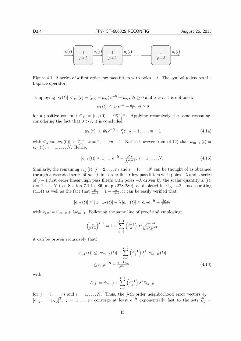
D3.4 FP7-ICT-600825 RECONFIG August 26, 2015
1
p l+
1
p l+
1
p l+
( )is t ( )1w t ( )2
w t ( )kw t...
Figure 4.1: A series of k first order low pass filters with poles −λ. The symbol p denotes theLaplace operator.
Employing |si (t)| < ρi (t) = (ρi0 − ρ∞) e−lt + ρ∞, ∀t ≥ 0 and λ > l, it is obtained:
|w1 (t)| ≤ w1e−lt + ρ∞
λ , ∀t ≥ 0
for a positive constant w1 := |w1 (0)| + ρi0−ρ∞λ−l . Applying recursively the same reasoning,
considering the fact that λ > l, it is concluded:
|wk (t)| ≤ wke−lt + ρ∞
λk , k = 1, . . . ,m− 1 (4.14)
with wk := |wk (0)| + wk−1λ−l , k = 2, . . . ,m − 1. Notice however from (4.12) that wm−1 (t) =
ei,1 (t), i = 1, . . . , N . Hence,
|ei,1 (t)| ≤ wm−1e−lt + ρ∞
λm−1 , i = 1, . . . , N . (4.15)
Similarly, the remaining ei,j (t), j = 2, . . . ,m and i = 1, . . . , N can be thought of as obtainedthrough a cascaded series of m− j first order linear low pass filters with poles −λ and a seriesof j − 1 first order linear high pass filters with poles −λ driven by the scalar quantity si (t),i = 1, . . . , N (see Section 7.1 in [86] at pp.278-280), as depicted in Fig. 4.2. Incorporating(4.14) as well as the fact that p
p+λ = 1 − λp+λ , it can be easily verified that:
|ei,2 (t)| ≤ |wm−2 (t)| + λ |ei,1 (t)| ≤ ei,2e−lt + 2ρ∞
λm−2
with ei,2 := wm−2 + λwm−1. Following the same line of proof and employing:
(p
p+λ
)j−1= 1 −
j−1∑k=1
(j−1
k
)λk pj−1−k
(p+λ)j−1
it can be proven recursively that:
|ei,j (t)| ≤ |wm−j (t)| +j−1∑k=1
(j−1
k
)λk |ei,j−k (t)|
≤ ei,je−lt + 2j−1ρ∞
λm−j (4.16)
with
ei,j := wm−j +j−1∑k=1
(j−1
k
)λkei,j−k
for j = 3, . . . ,m and i = 1, . . . , N . Thus, the j-th order neighborhood error vectors ej =[e1,j , . . . , eN,j ]T , j = 1, . . . ,m converge at least e−lt exponentially fast to the sets Ej =
43
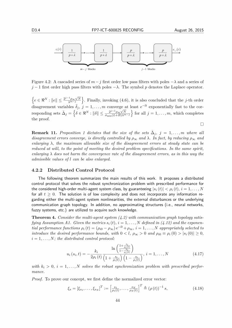
D3.4 FP7-ICT-600825 RECONFIG August 26, 2015
1
p l+
1
p l+
p
p l+
( )is t ( ),i j
e t......
m j- 1j -blocks blocks
p
p l+
Figure 4.2: A cascaded series of m− j first order low pass filters with poles −λ and a series ofj − 1 first order high pass filters with poles −λ. The symbol p denotes the Laplace operator.
e ∈ ℜN : ∥e∥ ≤ 2j−1ρ∞
√N
λm−j
. Finally, invoking (4.6), it is also concluded that the j-th order
disagreement variables δj , j = 1, . . . ,m converge at least e−lt exponentially fast to the cor-responding sets ∆j =
δ ∈ ℜN : ∥δ∥ ≤ 2j−1ρ∞
√N
σmin(L+B)λm−j
for all j = 1, . . . ,m, which completes
the proof.
Remark 11. Proposition 1 dictates that the size of the sets ∆j, j = 1, . . . ,m where alldisagreement errors converge, is directly controlled by ρ∞ and λ. In fact, by reducing ρ∞ andenlarging λ, the maximum allowable size of the disagreement errors at steady state can bereduced at will, to the point of meeting the desired problem specifications. In the same spirit,enlarging λ does not harm the convergence rate of the disagreement errors, as in this way theadmissible values of l can be also enlarged.
4.2.2 Distributed Control Protocol
The following theorem summarizes the main results of this work. It proposes a distributedcontrol protocol that solves the robust synchronization problem with prescribed performance forthe considered high-order multi-agent system class, by guaranteeing |si (t)| < ρi (t), i = 1, . . . , Nfor all t ≥ 0. The solution is of low complexity and does not incorporate any information re-garding either the multi-agent system nonlinearities, the external disturbances or the underlyingcommunication graph topology. In addition, no approximating structures (i.e., neural networks,fuzzy systems, etc.) are utilized to acquire such knowledge.
Theorem 4. Consider the multi-agent system (4.2) with communication graph topology satis-fying Assumption A1. Given the metrics si (t), i = 1, . . . , N defined in (4.12) and the exponen-tial performance functions ρi (t) = (ρi0 − ρ∞) e−lt +ρ∞, i = 1, . . . , N appropriately selected tointroduce the desired performance bounds, with 0 < l, ρ∞ > 0 and ρi0 ≡ ρi (0) > |si (0)| ≥ 0,i = 1, . . . , N ; the distributed control protocol:
ui (si, t) = − ki
2ρi (t)
ln(
1+ siρi(t)
1− siρi(t)
)(1 + si
ρi(t)
) (1 − si
ρi(t)
) , i = 1, . . . , N (4.17)
with ki > 0, i = 1, . . . , N solves the robust synchronization problem with prescribed perfor-mance.
Proof. To prove our concept, we first define the normalized error vector:
ξs = [ξs1 , . . . , ξsN ]T :=[
s1ρ1(t) , . . . ,
sNρN (t)
]T, (ρ (t))−1 s, (4.18)
44
D3.4 FP7-ICT-600825 RECONFIG August 26, 2015
where ρ (t) = diag ([ρ1 (t) , . . . , ρN (t)]) and s = [s1, . . . , sN ]T , as well as the generalized statevector ξ =
[xT , ξT
s
]T∈ ℜ(m+1)N with x = [x1, . . . , xm]T ∈ ℜmN . Differentiating ξ with
respect to time and substituting the system dynamics (4.2), it is obtained:
ξ =
x2...xm
F (x) +Gu+ d (t)(ρ (t))−1 (s− ρ (t) ξs)
. (4.19)
Differentiating (4.12) with respect to time and exploiting the dynamics of the agents from(4.5) and (4.11), s becomes:
s = (L+B)(F (x) +Gu+ d (t) − x0,m+1 (t)
+m−1∑k=1
(m−1
k
)λk (xk − x0,k (t))
). (4.20)
Substituting (4.20) and the distributed control protocol (4.17) in (4.19), the closed loop systemis obtained:
ξ = h (t, ξ)
=
x2...xm
F (x) −GK (ρ (t))−1 r (ξs) ε (ξs) + d (t)
(ρ (t))−1(
(L+B)(F (x)
−GK (ρ (t))−1 r (ξs) ε (ξs) + d (t) − x0,m+1 (t)
+m−1∑k=1
(m−1
k
)λk (xk − x0,k (t))
)− ρ (t) ξs
)
(4.21)
where
K = diag ([k1, . . . , kN ])ε (ξs) = [ε1 (ξs1) , . . . , εN (ξsN )]T
=[
12 ln
(1+ξs11−ξs1
), . . . , 1
2 ln(1+ξsN
1−ξsN
)]T(4.22)
r (ξs) = diag([
dε1(ξs1)dξs1
, . . . ,dεN(ξsN )
dξsN
])= diag
([1
(1+ξs1)(1−ξs1) , . . . ,1
(1+ξsN )(1−ξsN )
]). (4.23)
Finally, let us also define the open set:
Ωξ = ℜmN × (−1, 1) × · · · × (−1, 1)︸ ︷︷ ︸N times
.
45
D3.4 FP7-ICT-600825 RECONFIG August 26, 2015
In what follows, we proceed in two phases. First, the existence of a unique maximal solutionξ (t) of (4.21) over the set Ωξ for a time interval [0, τmax) (i.e., ξ (t) ∈ Ωξ, ∀t ∈ [0, τmax))is ensured. Then, it is proven that the proposed control scheme (4.17) guarantees, for allt ∈ [0, τmax): a) the boundedness of all closed loop signals of (4.21) and b) that ξ (t) remainsstrictly within a compact subset of Ωξ, leading by contradiction to τmax = ∞ and conse-quently to |si (t)| < ρi (t), i = 1, . . . , N for all t ≥ 0; thus completing the proof by exploitingProposition 1.
Phase A. The set Ωξ is nonempty and open. Moreover, the performance functions ρi (t),i = 1, . . . , N have been selected to satisfy ρi (0) > |si (0)|, i = 1, . . . , N . As a consequence,∣∣∣ si(0)
ρi(0)
∣∣∣ < 1, which results in ξ (0) ∈ Ωξ. Additionally, owing to the piecewise continuity andboundedness of d (t), (ρ (t))−1, ρ (t), x0,j (t), j = 1, . . . ,m+ 1 for all t ≥ 0 and the piecewisecontinuity of the system nonlinearities as well as of the control protocol over Ωξ, the righthand side of (4.21) suffices the hypotheses of Theorem 54 in [87] (pp.476), ensuring thus theexistence of a maximal solution ξ (t) of (4.21) on a time interval [0, τmax) such that ξ (t) ∈ Ωξ,∀t ∈ [0, τmax).
Phase B. It was proven in Phase A that ξ (t) ∈ Ωξ, ∀t ∈ [0, τmax) and more specificallythat:
ξsi (t) = si(t)ρi(t) ∈ (−1, 1) , i = 1, . . . , N (4.24)
for all t ∈ [0, τmax), from which it is obtained that si (t), i = 1, . . . , N are absolutely boundedby ρi (t), i = 1, . . . , N for all t ∈ [0, τmax). Thus, utilizing (4.16) from the proof of Proposition1, it is concluded that the neighborhood errors ei,j (t), i = 1, . . . , N and j = 1, . . . ,m evolvestrictly within the corresponding compact sets Ei,j =
ei,j ∈ ℜ : |ei,j | ≤ e⋆
i,j := ei,j + 2j−1ρ∞λm−j
,
i = 1, . . . , N and j = 1, . . . ,m for all t ∈ [0, τmax). Similarly, employing (4.6), (4.3) and theboundedness of the leader’s state x0 (t) and its derivatives up to m-th order, it is deduced:
x (t) ∈ Ωx ⊂ ℜmN , ∀t ∈ [0, τmax) (4.25)
with the compact set Ωx defined as follows:
Ωx =
x =
x1...xm
∈ ℜmN : ∥xj∥ ≤√N sup
t≥0
∣∣∣x(j−1)0 (t)
∣∣∣
+∑N
i=1e⋆
i,j
σmin(L+B) , ∀j = 1, . . . ,m
. (4.26)
To proceed, notice that the errors:
εi (ξsi) = 12 ln
(1+ξsi1−ξsi
), i = 1, . . . , N (4.27)
are well defined for all t ∈ [0, τmax) owing to (4.24). Moreover, according to Assumption A1,L + B is a nonsingular M-matrix. Hence, as the matrices G and K are diagonal with posi-tive entries, the product (L+B)GK is also a nonsingular M-matrix4. Therefore, invoking
4Notice that the right product of a matrix A with a positive definite diagonal matrix D corresponds to themultiplication of each column of A with the corresponding diagonal element of D. Thus, if A is an M-matrix,which is equivalent to all its principal minors being positive, then AD is also an M-matrix since the sign ofits principal minors are the same with those of A, owing to the positive definiteness of D.
46
D3.4 FP7-ICT-600825 RECONFIG August 26, 2015
Lemma 2, there exists a diagonal positive definite matrix P defined as P = (diag (q))−1 withq = ((L+B)GK)−1 1 and 1 := [1, . . . , 1]T ∈ ℜN .
To continue, let us define the positive definite and radially unbounded function:
Vε = 12ε
T (ξs)Pε (ξs) . (4.28)
Notice from (4.21), (4.22) and (4.23) that:
ε (ξs) = r (ξs) (ρ (t))−1(
(L+B)(F (x)
−GK (ρ (t))−1 r (ξs) ε (ξs) + d (t) − x0,m+1 (t)
+m−1∑k=1
(m−1
k
)λk (xk − x0,k (t))
)− ρ (t) ξs
). (4.29)
Hence, differentiating (4.28) with respect to time and substituting (4.29), it is obtained:
Vε = −εT (ξs) P r (ξs) (ρ (t))−1 (L + B) GK (ρ (t))−1 r (ξs) ε (ξs)
+εT (ξs) P r (ξs) (ρ (t))−1(
(L + B)(
F (x) + d (t) − x0,m+1 (t)
+m−1∑k=1
(m−1
k
)λk (xk − x0,k (t))
)− ρ (t) ξs
).
Employing the diagonality of r (ξs), (ρ (t))−1, P , G, K and expanding P (L+B)GK in itssymmetric and skew-symmetric part, it is deduced:
Vε = −12ε
T (ξs) r (ξs) (ρ (t))−1(P (L+B)GK
+KG (L+B)T P
)(ρ (t))−1 r (ξs) ε (ξs)
+εT (ξs) r (ξs) (ρ (t))−1 P
((L+B)
(F (x) + d (t)
−x0,m+1 (t) +m−1∑k=1
(m−1
k
)λk (xk − x0,k (t))
)− ρ (t) ξs
).
Owing to (4.25), the continuity of F (x), the boundedness of ξs by (4.24) and the boundednessof d (t), ρ (t) and x0,j (t), j = 1, . . . ,m + 1 either by assumption or by construction, theapplication of the Extreme Value Theorem guarantees the existence of a positive constant F ,independent of τmax, such that:
∥∥∥∥∥P(
(L+B)(F (x) + d (t) − x0,m+1 (t)
+m−1∑k=1
(m−1
k
)λk (xk − x0,k (t))
)− ρ (t) ξs
)∥∥∥∥∥ ≤ F
47
D3.4 FP7-ICT-600825 RECONFIG August 26, 2015
for all t ∈ [0, τmax). Furthermore, from Lemma 2 the matrixQ = P (L+B)GK+KG (L+B)T Pis positive definite. Thus, Vε becomes:
Vε ≤ −14ε
T (ξs) r (ξs) (ρ (t))−1Q (ρ (t))−1 r (ξs) ε (ξs)
− λQ
4
∥∥∥εT (ξs) r (ξs) (ρ (t))−1∥∥∥2
+∥∥∥εT (ξs) r (ξs) (ρ (t))−1
∥∥∥ Fwhere λQ := λmin
(P (L+B)GK +KG (L+B)T P
)with λmin (·) denoting the minimum
eigenvalue of a matrix. Moreover, it can be easily deduced that λmin (r (ξs)) ≥ 1 andλmin
((ρ (t))−1
)≥ λρ = 1
maxi∈1,...,Nρi0 by construction. Hence, after some straightforwardalgebraic manipulations, it is obtained:
Vε ≤ −λQλ2ρ
4 ∥ε (ξs)∥2 + F 2
λQ.
Therefore, Vε < 0 when ∥ε (ξs)∥ > 2FλQλρ
. Thus, it is concluded that:
∥ε (ξs)∥ ≤ ε = max
∥ε (ξs (0))∥ , 2FλQλρ
√λmax(P )λmin(P )
(4.30)
for all t ∈ [0, τmax), which by taking the inverse logarithmic function in (4.27), (i.e., thehyperbolic tangent function), leads to:
−1 < − tanh (ε) = ξ⋆s
≤ ξsi (t) ≤ ξ⋆s = tanh (ε) < 1 (4.31)
for i = 1, . . . , N and all t ∈ [0, τmax). Moreover, the control signals (4.17) remain bounded:
|ui (si, t)| ≤ ui = kiερ∞(1+tanh(ε))(1−tanh(ε)) , i = 1, . . . , N
for all t ∈ [0, τmax).Up to this point, what remains to be shown is that τmax can be extended to ∞. In this
direction, notice by (4.31) that ξ (t) ∈ Ω′ξ, ∀t ∈ [0, τmax), where the set:
Ω′ξ = Ωx ×
[ξ⋆
s, ξ
⋆s
]Nis a nonempty and compact subset of Ωξ. Hence, assuming τmax < ∞ and since Ω′
ξ ⊂ Ωξ,Proposition C.3.6 in [87] (pp.481) dictates the existence of a time instant t′ ∈ [0, τmax) suchthat ξ
(t
′)/∈ Ω′
ξ, which is a clear contradiction. Therefore, τmax = ∞. Thus, all closed loopsignals remain bounded and moreover ξ (t) ∈ Ω′
ξ ⊂ Ωξ, ∀t ≥ 0. Finally, multiplying (4.31) byρi (t), it is also concluded:
−ρi (t) < ξ⋆sρi (t) ≤ si (t) ≤ ξ
⋆sρi (t) < ρi (t) , i = 1, . . . , N (4.32)
for all t ≥ 0 and consequently, owing to Proposition 1, the solution of the robust synchroniza-tion control problem with prescribed performance for the considered multi-agent system.
In the sequel, several remarks are presented that provide intuitive explanations on the controldesign procedure and reveal its intriguing properties.
48
D3.4 FP7-ICT-600825 RECONFIG August 26, 2015
Design Philosophy
As stated in Proposition 1, a sufficient condition to guarantee prescribed transient and steadystate performance bounds on the disagreement variables δj , j = 1, . . . ,m is to enforce si (t),i = 1, . . . , N to evolve strictly within the envelope constructed with the aid of the exponentialperformance functions ρi (t) = (ρi0 − ρ∞) e−lt + ρ∞, i = 1, . . . , N . Stated otherwise, |si (t)| <ρi (t) for all t ≥ 0 and i = 1, . . . , N or equivalently −1 < ξsi (t) ≡ si(t)
ρi(t) < 1 for all t ≥ 0 andi = 1, . . . , N . Modulating ξsi (t) via the logarithmic function 1
2 ln(
1+⋆1−⋆
), which actually stands
for the inverse hyperbolic tangent function tanh−1 (⋆), and selecting ρi (0) > |si (0)|, the signalsεi (t) = 1
2 ln(1+ξsi (t)
1−ξsi (t)
), i = 1, . . . , N are initially well defined. It is not difficult to verify that
maintaining the boundedness of εi (t), i = 1, . . . , N is equivalent to guaranteeing |si (t)| < ρi (t),i = 1, . . . , N for all t ≥ 0. Therefore, the problem at hand can be visualized as minimizing thequadratic and positive definite objective function Vε = 1
2εT (ξs)Pε (ξs) within the feasible region
defined via |ξsi (t)| < 1, i = 1, . . . , N for all t ≥ 0. A careful inspection of the proposed controller(4.17) reveals that it actually operates similarly to barrier functions in constrained optimization,admitting high negative or positive values depending on whether si (t) → ρi (t) or si (t) → −ρi (t)respectively; eventually not permitting si (t) from reaching the performance boundaries.
Decentralization and Structural Complexity
The proposed control protocol for the generic class of multi-agent systems considered herein,is decentralized in the sense that each agent utilizes only local relative state information from itsneighborhood set to calculate its own control signal. Moreover, it does not incorporate any priorknowledge of the model nonlinearities/disturbances or even of some corresponding upper/lowerbounding functions, relaxing thus significantly the key assumptions made in the related literature.Additionally, no approximating structures (i.e., neural networks, fuzzy systems, etc.) have beenemployed to acquire such knowledge. Furthermore, no hard calculations (neither analytic nornumerical) are required to produce the control signal, thus making its distributed implementationstraightforward. Therefore, the proposed synchronization protocol besides being decentralized,exhibits low structural complexity as well.
Robust Prescribed Performance
From the proof of Theorem 4, it can be deduced that the proposed control scheme achievessynchronization with prescribed transient and steady state performance for the considered classof high-order nonlinear multi-agent systems without residing in the need of rendering the uniformbound of ∥ε (t)∥ (i.e., ε in (4.30)) arbitrarily small, by adopting extreme values of the controlgains ki, i = 1, ..., N . More specifically, (4.31) and consequently (4.32), which encapsulates theprescribed performance notion, hold no matter how large the finite bound ε is. In the same spirit,large model uncertainties can be compensated for, as they affect only the size of ε through F , leav-ing unaltered the achieved stability properties. Hence, the performance bounds, which are solelydetermined by the performance functions ρi (t), i = 1, . . . , N becomes isolated against modeluncertainties, extending greatly the robustness of the proposed control scheme. Furthermore, andcontrary to the standard distributed control schemes for static graphs, whose convergence rate isdictated by the connectivity level (i.e., the smallest singular value of L+B), the transient responseof the proposed scheme is independent of the underlying topology.
49
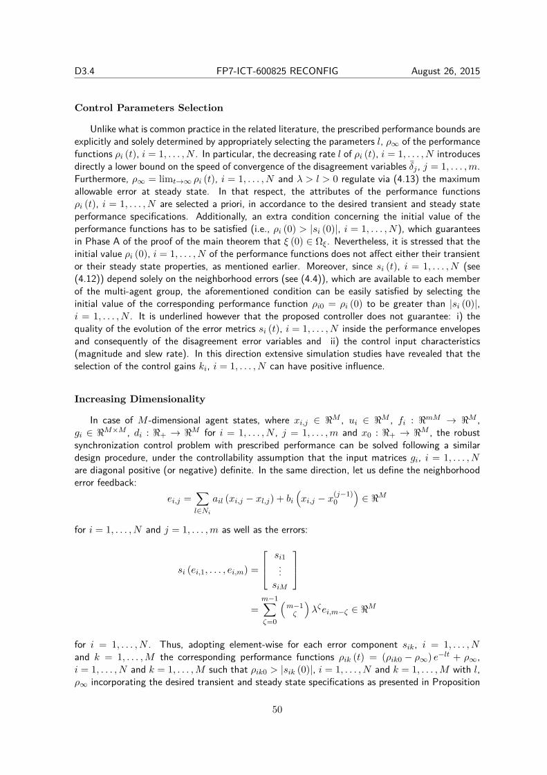
D3.4 FP7-ICT-600825 RECONFIG August 26, 2015
Control Parameters Selection
Unlike what is common practice in the related literature, the prescribed performance bounds areexplicitly and solely determined by appropriately selecting the parameters l, ρ∞ of the performancefunctions ρi (t), i = 1, . . . , N . In particular, the decreasing rate l of ρi (t), i = 1, . . . , N introducesdirectly a lower bound on the speed of convergence of the disagreement variables δj , j = 1, . . . ,m.Furthermore, ρ∞ = limt→∞ ρi (t), i = 1, . . . , N and λ > l > 0 regulate via (4.13) the maximumallowable error at steady state. In that respect, the attributes of the performance functionsρi (t), i = 1, . . . , N are selected a priori, in accordance to the desired transient and steady stateperformance specifications. Additionally, an extra condition concerning the initial value of theperformance functions has to be satisfied (i.e., ρi (0) > |si (0)|, i = 1, . . . , N), which guaranteesin Phase A of the proof of the main theorem that ξ (0) ∈ Ωξ. Nevertheless, it is stressed that theinitial value ρi (0), i = 1, . . . , N of the performance functions does not affect either their transientor their steady state properties, as mentioned earlier. Moreover, since si (t), i = 1, . . . , N (see(4.12)) depend solely on the neighborhood errors (see (4.4)), which are available to each memberof the multi-agent group, the aforementioned condition can be easily satisfied by selecting theinitial value of the corresponding performance function ρi0 = ρi (0) to be greater than |si (0)|,i = 1, . . . , N . It is underlined however that the proposed controller does not guarantee: i) thequality of the evolution of the error metrics si (t), i = 1, . . . , N inside the performance envelopesand consequently of the disagreement error variables and ii) the control input characteristics(magnitude and slew rate). In this direction extensive simulation studies have revealed that theselection of the control gains ki, i = 1, . . . , N can have positive influence.
Increasing Dimensionality
In case of M -dimensional agent states, where xi,j ∈ ℜM , ui ∈ ℜM , fi : ℜmM → ℜM ,gi ∈ ℜM×M , di : ℜ+ → ℜM for i = 1, . . . , N , j = 1, . . . ,m and x0 : ℜ+ → ℜM , the robustsynchronization control problem with prescribed performance can be solved following a similardesign procedure, under the controllability assumption that the input matrices gi, i = 1, . . . , Nare diagonal positive (or negative) definite. In the same direction, let us define the neighborhooderror feedback:
ei,j =∑l∈Ni
ail (xi,j − xl,j) + bi
(xi,j − x
(j−1)0
)∈ ℜM
for i = 1, . . . , N and j = 1, . . . ,m as well as the errors:
si (ei,1, . . . , ei,m) =
si1...
siM
=
m−1∑ζ=0
(m−1
ζ
)λζei,m−ζ ∈ ℜM
for i = 1, . . . , N . Thus, adopting element-wise for each error component sik, i = 1, . . . , Nand k = 1, . . . ,M the corresponding performance functions ρik (t) = (ρik0 − ρ∞) e−lt + ρ∞,i = 1, . . . , N and k = 1, . . . ,M such that ρik0 > |sik (0)|, i = 1, . . . , N and k = 1, . . . ,M with l,ρ∞ incorporating the desired transient and steady state specifications as presented in Proposition
50
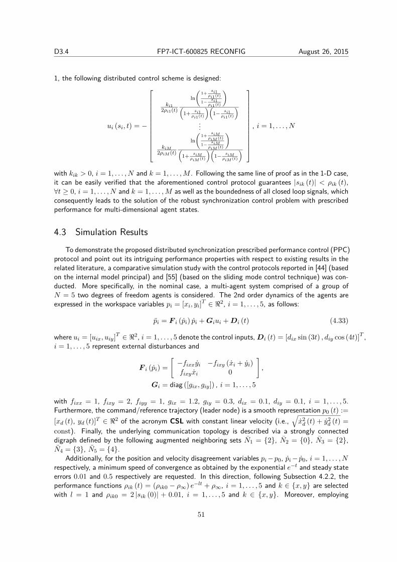
D3.4 FP7-ICT-600825 RECONFIG August 26, 2015
1, the following distributed control scheme is designed:
ui (si, t) = −
ki12ρi1(t)
ln(
1+ si1ρi1(t)
1− si1ρi1(t)
)(
1+ si1ρi1(t)
)(1− si1
ρi1(t)
)...
kiM2ρiM (t)
ln(
1+siM
ρiM (t)1−
siMρiM (t)
)(
1+ siMρiM (t)
)(1− siM
ρiM (t)
)
, i = 1, . . . , N
with kik > 0, i = 1, . . . , N and k = 1, . . . ,M . Following the same line of proof as in the 1-D case,it can be easily verified that the aforementioned control protocol guarantees |sik (t)| < ρik (t),∀t ≥ 0, i = 1, . . . , N and k = 1, . . . ,M as well as the boundedness of all closed loop signals, whichconsequently leads to the solution of the robust synchronization control problem with prescribedperformance for multi-dimensional agent states.
4.3 Simulation Results
To demonstrate the proposed distributed synchronization prescribed performance control (PPC)protocol and point out its intriguing performance properties with respect to existing results in therelated literature, a comparative simulation study with the control protocols reported in [44] (basedon the internal model principal) and [55] (based on the sliding mode control technique) was con-ducted. More specifically, in the nominal case, a multi-agent system comprised of a group ofN = 5 two degrees of freedom agents is considered. The 2nd order dynamics of the agents areexpressed in the workspace variables pi = [xi, yi]T ∈ ℜ2, i = 1, . . . , 5, as follows:
pi = F i (pi) pi + Giui + Di (t) (4.33)
where ui = [uix, uiy]T ∈ ℜ2, i = 1, . . . , 5 denote the control inputs, Di (t) = [dix sin (3t) , diy cos (4t)]T ,i = 1, . . . , 5 represent external disturbances and
F i (pi) =[
−fixxyi −fixy (xi + yi)fixyxi 0
],
Gi = diag ([gix, giy]) , i = 1, . . . , 5
with fixx = 1, fixy = 2, fiyy = 1, gix = 1.2, giy = 0.3, dix = 0.1, diy = 0.1, i = 1, . . . , 5.Furthermore, the command/reference trajectory (leader node) is a smooth representation p0 (t) :=[xd (t), yd (t)]T ∈ ℜ2 of the acronym CSL with constant linear velocity (i.e.,
√x2
d (t) + y2d (t) =
const). Finally, the underlying communication topology is described via a strongly connecteddigraph defined by the following augmented neighboring sets N1 = 2, N2 = 0, N3 = 2,N4 = 3, N5 = 4.
Additionally, for the position and velocity disagreement variables pi −p0, pi − p0, i = 1, . . . , Nrespectively, a minimum speed of convergence as obtained by the exponential e−t and steady stateerrors 0.01 and 0.5 respectively are requested. In this direction, following Subsection 4.2.2, theperformance functions ρik (t) = (ρik0 − ρ∞) e−lt + ρ∞, i = 1, . . . , 5 and k ∈ x, y are selectedwith l = 1 and ρik0 = 2 |sik (0)| + 0.01, i = 1, . . . , 5 and k ∈ x, y. Moreover, employing
51
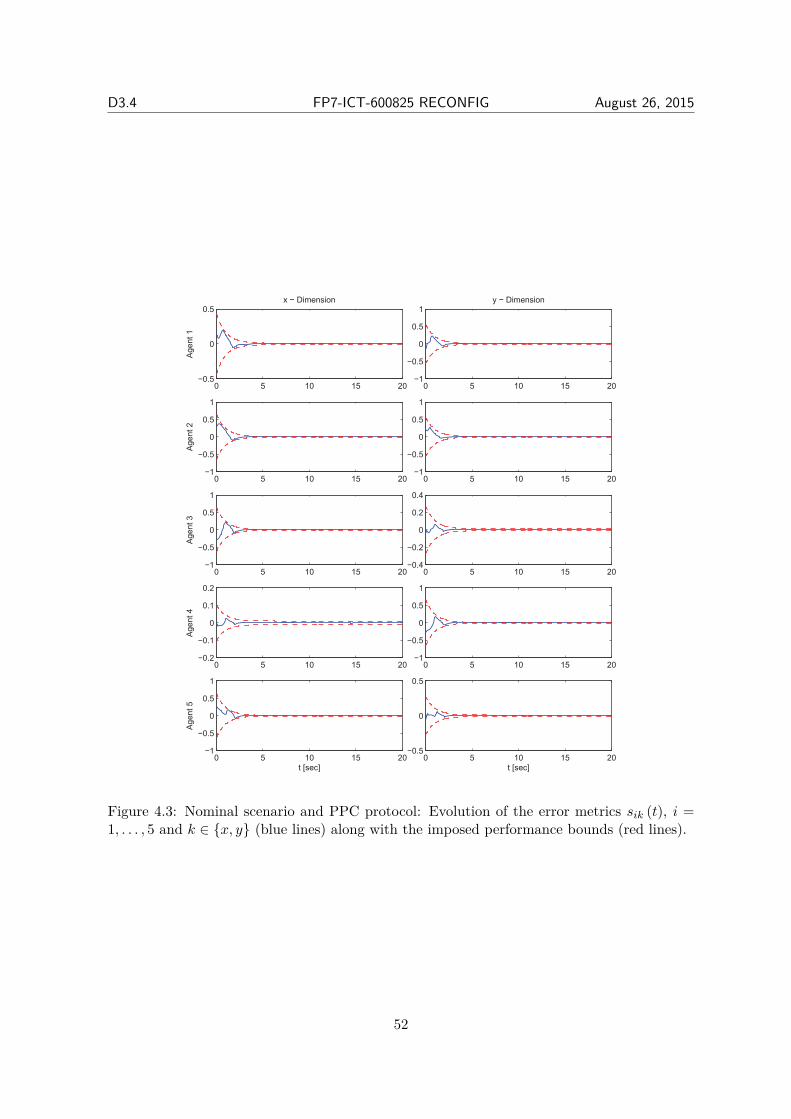
D3.4 FP7-ICT-600825 RECONFIG August 26, 2015
0 5 10 15 20−0.5
0
0.5x − Dimension
Agent
1
0 5 10 15 20−1
−0.5
0
0.5
1y − Dimension
0 5 10 15 20−1
−0.5
0
0.5
1
Agent
2
0 5 10 15 20−1
−0.5
0
0.5
1
0 5 10 15 20−1
−0.5
0
0.5
1
Agent
3
0 5 10 15 20−0.4
−0.2
0
0.2
0.4
0 5 10 15 20−0.2
−0.1
0
0.1
0.2
Agent
4
0 5 10 15 20−1
−0.5
0
0.5
1
0 5 10 15 20−1
−0.5
0
0.5
1
Agent
5
t [sec]
0 5 10 15 20−0.5
0
0.5
t [sec]
Figure 4.3: Nominal scenario and PPC protocol: Evolution of the error metrics sik (t), i =1, . . . , 5 and k ∈ x, y (blue lines) along with the imposed performance bounds (red lines).
52
D3.4 FP7-ICT-600825 RECONFIG August 26, 2015
−0.3 −0.2 −0.1 0 0.1 0.2 0.3 0.4 0.5 0.6 0.7
−0.3
−0.2
−0.1
0
0.1
0.2
0.3
0.4
x [m]
y [
m]
Leader
Agent 1
Agent 2
Agent 3
Agent 4
Agent 5
Figure 4.4: Nominal scenario and PPC protocol: Trace of the agents in the workspace.
0 5 10 15 20−0.5
0
0.5
1x − Dimension
Positio
n
0 5 10 15 20−0.4
−0.2
0
0.2
0.4
0.6y − Dimension
Leader
Agent 1
Agent 2
Agent 3
Agent 4
Agent 5
0 5 10 15 20−0.4
−0.2
0
0.2
0.4
Velo
city
t [sec]
0 5 10 15 20−0.4
−0.2
0
0.2
0.4
t [sec]
Figure 4.5: Nominal scenario and PPC protocol: Evolution of the position and velocity statesof the multi agent system.
53
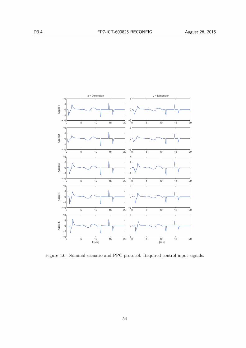
D3.4 FP7-ICT-600825 RECONFIG August 26, 2015
0 5 10 15 20−10
−5
0
5
10x − Dimension
Agent
1
0 5 10 15 20−5
0
5y − Dimension
0 5 10 15 20−10
−5
0
5
10
Agent
2
0 5 10 15 20−5
0
5
0 5 10 15 20−10
−5
0
5
10
Agent
3
0 5 10 15 20−4
−2
0
2
4
0 5 10 15 20−10
−5
0
5
10
Agent
4
0 5 10 15 20−5
0
5
0 5 10 15 20−10
−5
0
5
10
Agent
5
t [sec]
0 5 10 15 20−5
0
5
t [sec]
Figure 4.6: Nominal scenario and PPC protocol: Required control input signals.
54
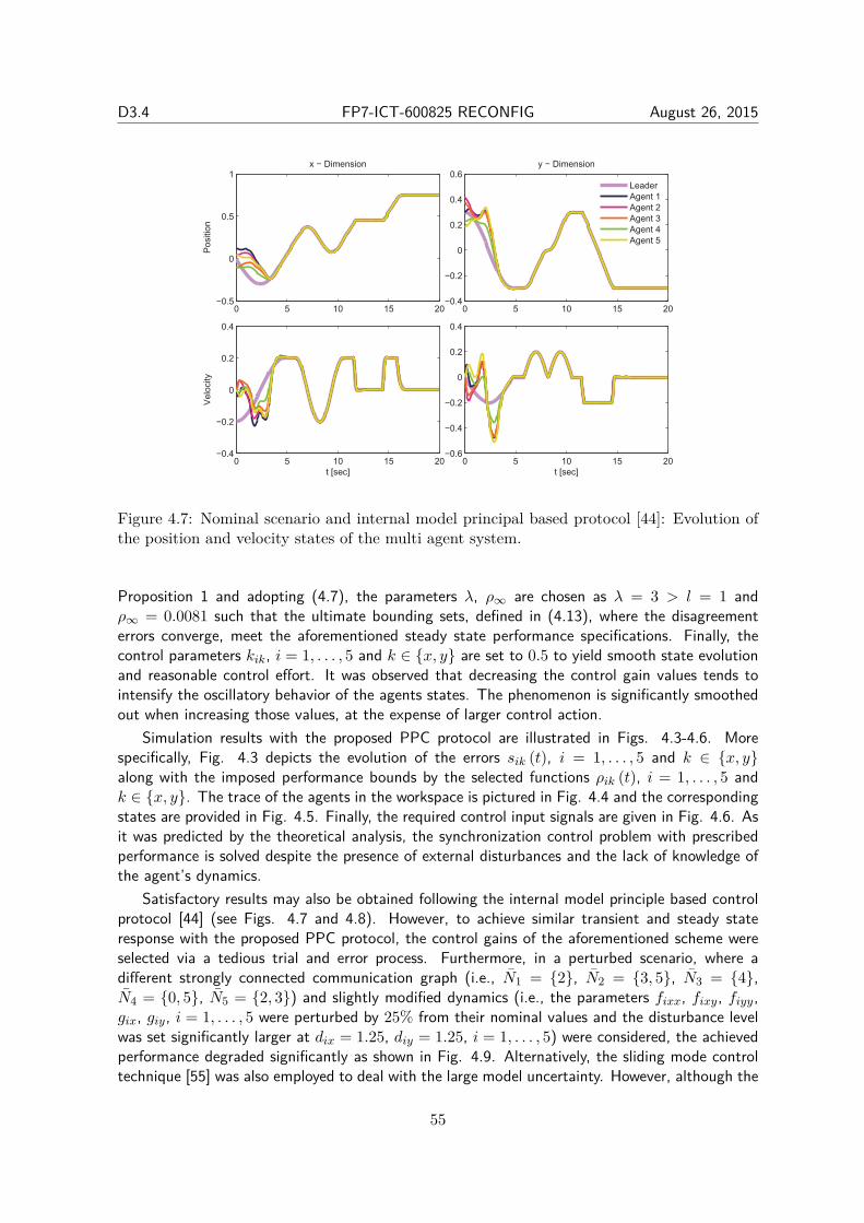
D3.4 FP7-ICT-600825 RECONFIG August 26, 2015
0 5 10 15 20−0.5
0
0.5
1x − Dimension
Positio
n
0 5 10 15 20−0.4
−0.2
0
0.2
0.4
0.6y − Dimension
Leader
Agent 1
Agent 2
Agent 3
Agent 4
Agent 5
0 5 10 15 20−0.4
−0.2
0
0.2
0.4
Velo
city
t [sec]
0 5 10 15 20−0.6
−0.4
−0.2
0
0.2
0.4
t [sec]
Figure 4.7: Nominal scenario and internal model principal based protocol [44]: Evolution ofthe position and velocity states of the multi agent system.
Proposition 1 and adopting (4.7), the parameters λ, ρ∞ are chosen as λ = 3 > l = 1 andρ∞ = 0.0081 such that the ultimate bounding sets, defined in (4.13), where the disagreementerrors converge, meet the aforementioned steady state performance specifications. Finally, thecontrol parameters kik, i = 1, . . . , 5 and k ∈ x, y are set to 0.5 to yield smooth state evolutionand reasonable control effort. It was observed that decreasing the control gain values tends tointensify the oscillatory behavior of the agents states. The phenomenon is significantly smoothedout when increasing those values, at the expense of larger control action.
Simulation results with the proposed PPC protocol are illustrated in Figs. 4.3-4.6. Morespecifically, Fig. 4.3 depicts the evolution of the errors sik (t), i = 1, . . . , 5 and k ∈ x, yalong with the imposed performance bounds by the selected functions ρik (t), i = 1, . . . , 5 andk ∈ x, y. The trace of the agents in the workspace is pictured in Fig. 4.4 and the correspondingstates are provided in Fig. 4.5. Finally, the required control input signals are given in Fig. 4.6. Asit was predicted by the theoretical analysis, the synchronization control problem with prescribedperformance is solved despite the presence of external disturbances and the lack of knowledge ofthe agent’s dynamics.
Satisfactory results may also be obtained following the internal model principle based controlprotocol [44] (see Figs. 4.7 and 4.8). However, to achieve similar transient and steady stateresponse with the proposed PPC protocol, the control gains of the aforementioned scheme wereselected via a tedious trial and error process. Furthermore, in a perturbed scenario, where adifferent strongly connected communication graph (i.e., N1 = 2, N2 = 3, 5, N3 = 4,N4 = 0, 5, N5 = 2, 3) and slightly modified dynamics (i.e., the parameters fixx, fixy, fiyy,gix, giy, i = 1, . . . , 5 were perturbed by 25% from their nominal values and the disturbance levelwas set significantly larger at dix = 1.25, diy = 1.25, i = 1, . . . , 5) were considered, the achievedperformance degraded significantly as shown in Fig. 4.9. Alternatively, the sliding mode controltechnique [55] was also employed to deal with the large model uncertainty. However, although the
55
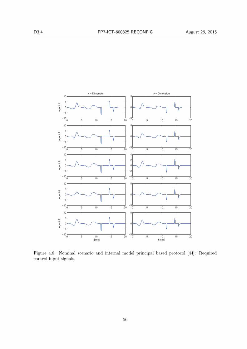
D3.4 FP7-ICT-600825 RECONFIG August 26, 2015
0 5 10 15 20−10
−5
0
5
10x − Dimension
Agent
1
0 5 10 15 20−5
0
5y − Dimension
0 5 10 15 20−10
−5
0
5
10
Agent
2
0 5 10 15 20−5
0
5
0 5 10 15 20−10
−5
0
5
10
Agent
3
0 5 10 15 20−4
−2
0
2
4
0 5 10 15 20−10
−5
0
5
10
Agent
4
0 5 10 15 20−5
0
5
0 5 10 15 20−10
−5
0
5
10
Agent
5
t [sec]
0 5 10 15 20−5
0
5
t [sec]
Figure 4.8: Nominal scenario and internal model principal based protocol [44]: Requiredcontrol input signals.
56
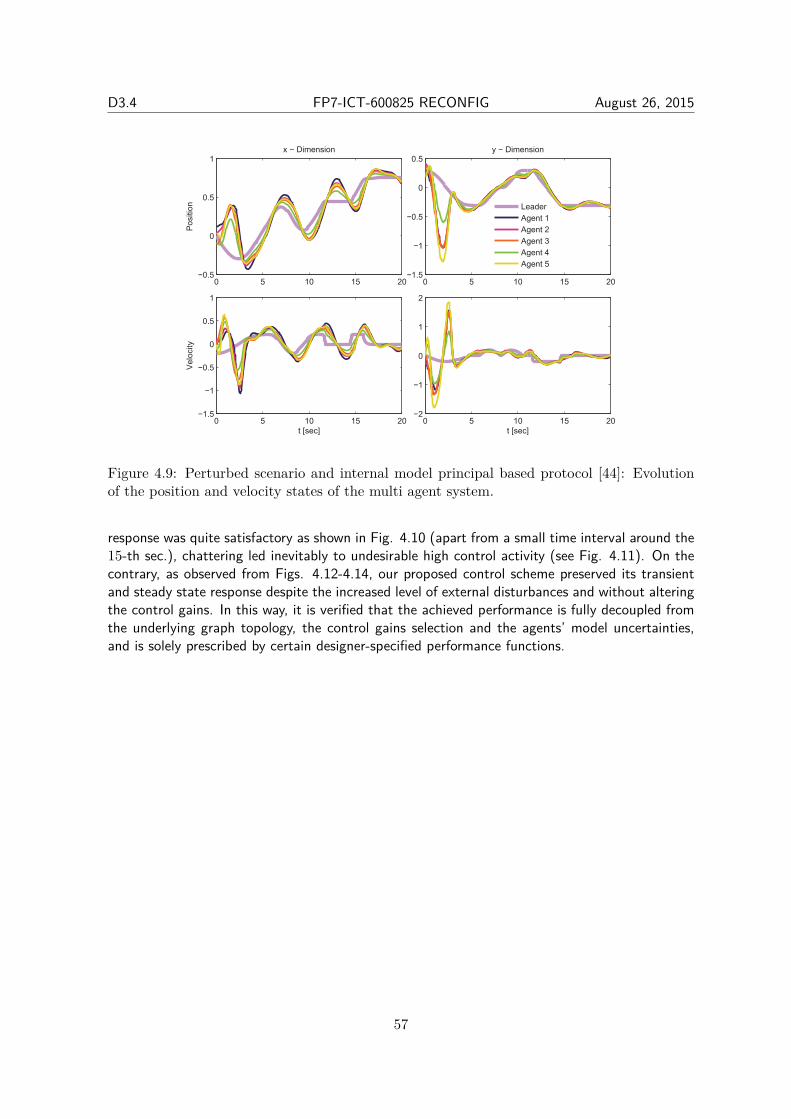
D3.4 FP7-ICT-600825 RECONFIG August 26, 2015
0 5 10 15 20−0.5
0
0.5
1x − Dimension
Positio
n
0 5 10 15 20−1.5
−1
−0.5
0
0.5y − Dimension
0 5 10 15 20−1.5
−1
−0.5
0
0.5
1
Velo
city
t [sec]
0 5 10 15 20−2
−1
0
1
2
t [sec]
Leader
Agent 1
Agent 2
Agent 3
Agent 4
Agent 5
Figure 4.9: Perturbed scenario and internal model principal based protocol [44]: Evolutionof the position and velocity states of the multi agent system.
response was quite satisfactory as shown in Fig. 4.10 (apart from a small time interval around the15-th sec.), chattering led inevitably to undesirable high control activity (see Fig. 4.11). On thecontrary, as observed from Figs. 4.12-4.14, our proposed control scheme preserved its transientand steady state response despite the increased level of external disturbances and without alteringthe control gains. In this way, it is verified that the achieved performance is fully decoupled fromthe underlying graph topology, the control gains selection and the agents’ model uncertainties,and is solely prescribed by certain designer-specified performance functions.
57
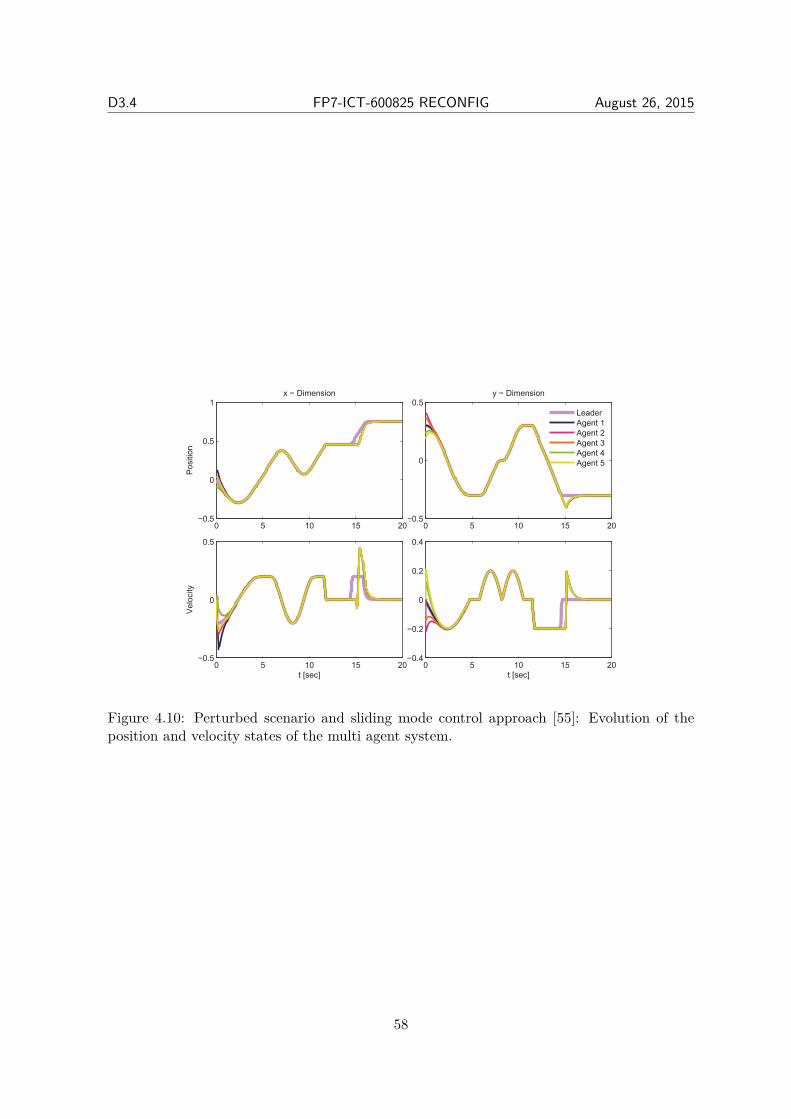
D3.4 FP7-ICT-600825 RECONFIG August 26, 2015
0 5 10 15 20−0.5
0
0.5
1x − Dimension
Positio
n
0 5 10 15 20−0.5
0
0.5y − Dimension
Leader
Agent 1
Agent 2
Agent 3
Agent 4
Agent 5
0 5 10 15 20−0.5
0
0.5
Velo
city
t [sec]
0 5 10 15 20−0.4
−0.2
0
0.2
0.4
t [sec]
Figure 4.10: Perturbed scenario and sliding mode control approach [55]: Evolution of theposition and velocity states of the multi agent system.
58
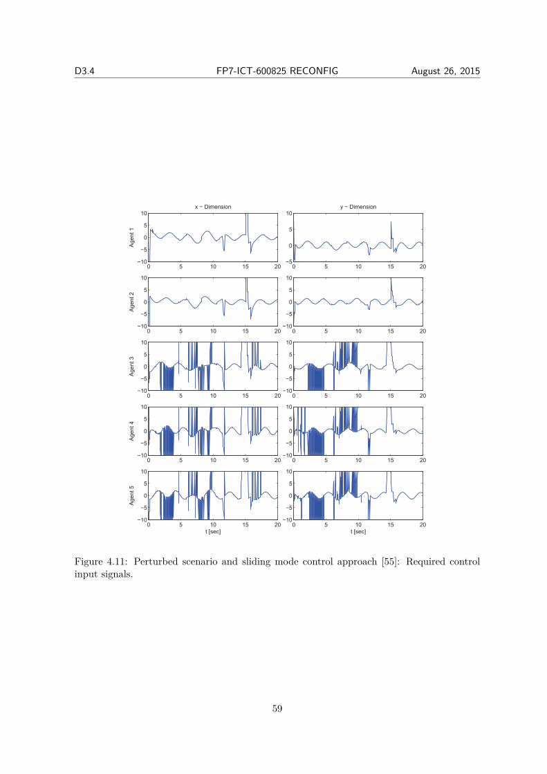
D3.4 FP7-ICT-600825 RECONFIG August 26, 2015
0 5 10 15 20−10
−5
0
5
10x − Dimension
Agent
1
0 5 10 15 20−5
0
5
10y − Dimension
0 5 10 15 20−10
−5
0
5
10
Agent
2
0 5 10 15 20−10
−5
0
5
10
0 5 10 15 20−10
−5
0
5
10
Agent
3
0 5 10 15 20−10
−5
0
5
10
0 5 10 15 20−10
−5
0
5
10
Agent
4
0 5 10 15 20−10
−5
0
5
10
0 5 10 15 20−10
−5
0
5
10
Agent
5
t [sec]
0 5 10 15 20−10
−5
0
5
10
t [sec]
Figure 4.11: Perturbed scenario and sliding mode control approach [55]: Required controlinput signals.
59
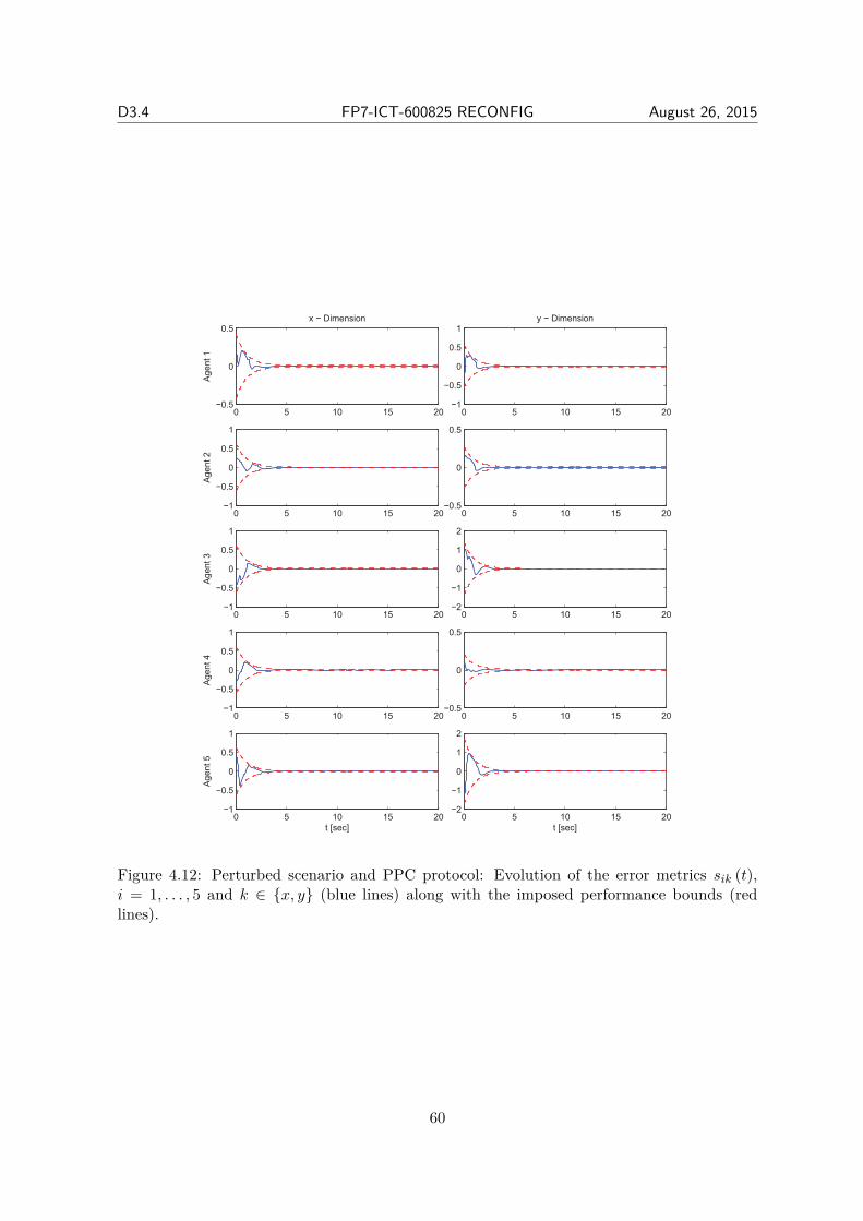
D3.4 FP7-ICT-600825 RECONFIG August 26, 2015
0 5 10 15 20−0.5
0
0.5x − Dimension
Agent
1
0 5 10 15 20−1
−0.5
0
0.5
1y − Dimension
0 5 10 15 20−1
−0.5
0
0.5
1
Agent
2
0 5 10 15 20−0.5
0
0.5
0 5 10 15 20−1
−0.5
0
0.5
1
Agent
3
0 5 10 15 20−2
−1
0
1
2
0 5 10 15 20−1
−0.5
0
0.5
1
Agent
4
0 5 10 15 20−0.5
0
0.5
0 5 10 15 20−1
−0.5
0
0.5
1
Agent
5
t [sec]
0 5 10 15 20−2
−1
0
1
2
t [sec]
Figure 4.12: Perturbed scenario and PPC protocol: Evolution of the error metrics sik (t),i = 1, . . . , 5 and k ∈ x, y (blue lines) along with the imposed performance bounds (redlines).
60
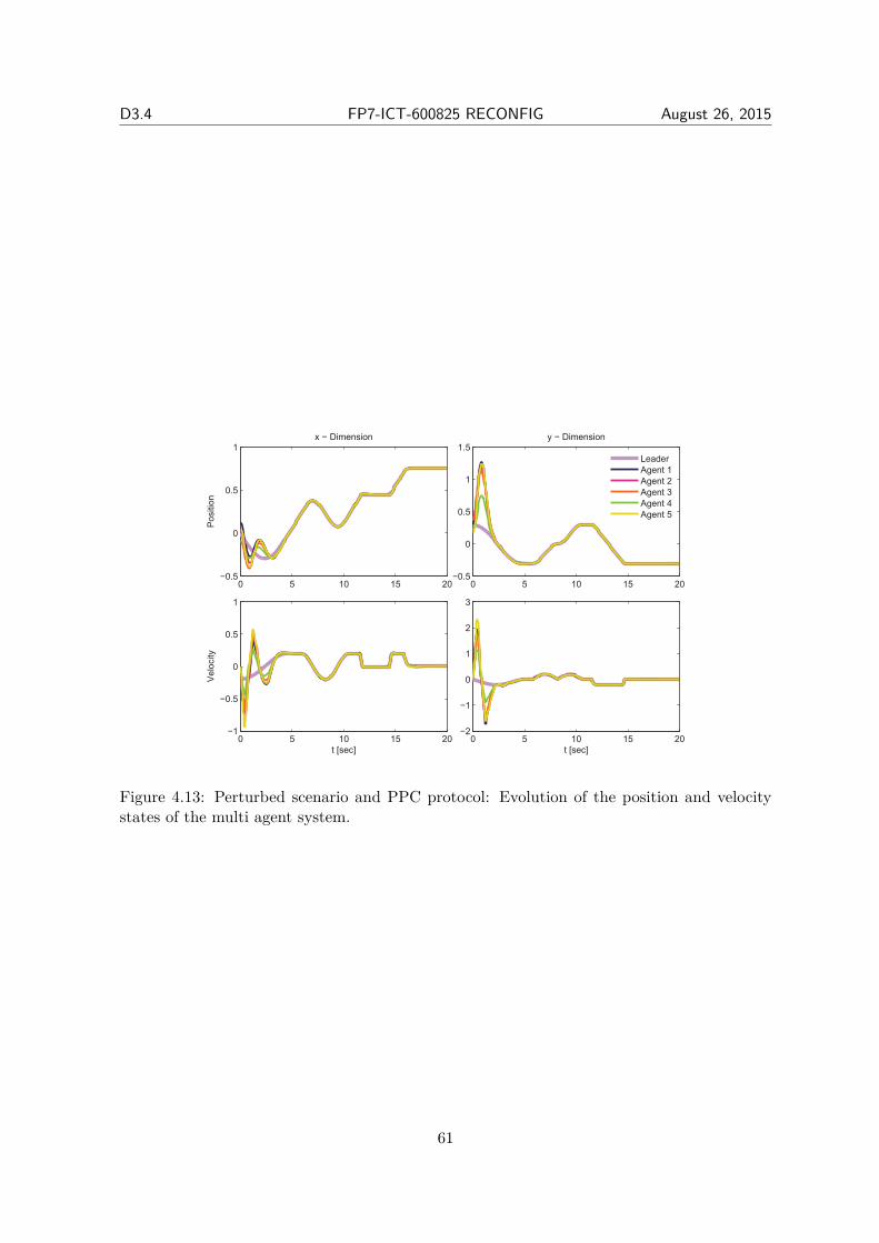
D3.4 FP7-ICT-600825 RECONFIG August 26, 2015
0 5 10 15 20−0.5
0
0.5
1x − Dimension
Positio
n
0 5 10 15 20−0.5
0
0.5
1
1.5y − Dimension
Leader
Agent 1
Agent 2
Agent 3
Agent 4
Agent 5
0 5 10 15 20−1
−0.5
0
0.5
1
Velo
city
t [sec]
0 5 10 15 20−2
−1
0
1
2
3
t [sec]
Figure 4.13: Perturbed scenario and PPC protocol: Evolution of the position and velocitystates of the multi agent system.
61
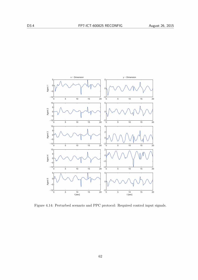
D3.4 FP7-ICT-600825 RECONFIG August 26, 2015
0 5 10 15 20−10
−5
0
5x − Dimension
Agent
1
0 5 10 15 20−5
0
5y − Dimension
0 5 10 15 20−10
−5
0
5
10
Agent
2
0 5 10 15 20−5
0
5
0 5 10 15 20−10
−5
0
5
10
Agent
3
0 5 10 15 20−2
0
2
4
0 5 10 15 20−10
−5
0
5
10
Agent
4
0 5 10 15 20−4
−2
0
2
0 5 10 15 20−10
−5
0
5
Agent
5
t [sec]
0 5 10 15 20−5
0
5
t [sec]
Figure 4.14: Perturbed scenario and PPC protocol: Required control input signals.
62
Appendix A
Prescribed Performance
The concepts and techniques of prescribed performance control, recently developed in [67,68]for nonlinear systems, are innovatively adapted in Chapters 2-4 to deal with the considered controlproblems therein. Prescribed performance characterizes the behavior where the tracking errorconverges to a predefined arbitrarily small residual set with convergence rate no less than a certainpredefined value. For completeness and compactness of presentation, this appendix summarizespreliminary knowledge on prescribed performance.
In that respect, consider a generic scalar tracking error e (t). Prescribed performance isachieved if e (t) evolves strictly within a predefined region that is bounded by certain functions oftime. The mathematical expression of prescribed performance is given by the following inequalities:
ρL (t) < e (t) < ρU (t) , ∀t ≥ 0 (A.1)
where ρL (t), ρU (t) are smooth and bounded functions of time satisfying limt→∞ ρU (t) >limt→∞ ρL (t), called performance functions. The aforementioned statements are clearly illus-trated in the following figure for exponential performance functions ρi (t) = (ρi0 − ρi∞) e−lit+ρi∞with appropriately chosen constants ρi0, ρi∞, li, i ∈ L,U. More specifically, the constantsρL0 = ρL (0), ρU0 = ρU (0) are selected such that ρL0 < e (0) < ρU0. Furthermore, the con-stants ρL∞ = limt→∞ ρL (t), ρU∞ = limt→∞ ρU (t) represent the maximum allowable range ofthe tracking error e (t) at steady state, which may even be set arbitrarily small to a value reflectingthe resolution of the measurement device, thus achieving practical convergence of e (t) to zero.Moreover, the decreasing rate of ρL (t), ρU (t) which is affected by the constants lL, lU in thiscase, introduces a lower bound on the required speed of convergence of e (t). Therefore, theappropriate selection of the performance functions ρL (t), ρU (t) imposes transient and steadystate performance characteristics on the tracking error e (t).
63
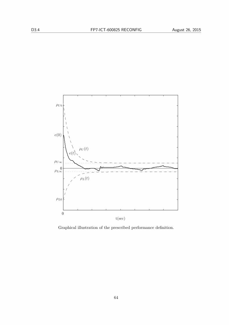
D3.4 FP7-ICT-600825 RECONFIG August 26, 2015
0
0
t(sec)
ρU (t)
ρL(t)
e(t)
ρU0
ρL0
ρU∞
ρL∞
e(0)
Graphical illustration of the prescribed performance definition.
64
Appendix B
Dynamical SystemsConsider the initial value problem:
ξ = h (t, ξ) , ξ (0) = ξ0 ∈ Ωξ (B.1)
with h : ℜ+ × Ωξ → ℜn, where Ωξ ⊂ ℜn is a non-empty open set.
Definition 1. [87] A solution ξ (t) of the initial value problem (B.1) is maximal if it has noproper right extension that is also a solution of (B.1).
As an example, consider the initial value problem ξ = ξ2, ξ (0) = 1 over ℜ (i.e., Ωξ = ℜ),with solution ξ (t) = 1
1−t , ∀t ∈ [0, 1). The solution is maximal since it cannot be defined fort > 1. Stated otherwise, there is no proper extension of ξ (t) to the right of t = 1 that is also asolution of the original initial value problem.
Theorem 5. [87] Consider the initial value problem (B.1). Assume that h (t, ξ) is: a) locallyLipschitz on ξ for almost all t ∈ ℜ+, b) piecewise continuous on t for each fixed ξ ∈ Ωξ andc) locally integrable on t for each fixed ξ ∈ Ωξ. Then, there exists a maximal solution ξ (t) of(B.1) on the time interval [0, τmax) with τmax > 0 such that ξ (t) ∈ Ωξ, ∀t ∈ [0, τmax).
Proposition 2. [87] Assume that the hypotheses of Theorem 5 hold. For a maximal solutionξ (t) on the time interval [0, τmax) with τmax < ∞ and for any compact set Ω′
ξ ⊂ Ωξ thereexists a time instant t′ ∈ [0, τmax) such that ξ (t′) /∈ Ω′
ξ.
65
Bibliography
[1] I. D. Couzin, J. Krause, N. R. Franks, and S. A. Levin, “Effective leadership and decision-making in animal groups on the move,” Nature, vol. 433, no. 7025, pp. 513–516, 2005.
[2] G. Pereira, B. Pimentel, L. Chaimowicz, and M. Campos, “Coordination of multiple mobilerobots in an object carrying task using implicit communication,” in Proceedings of the IEEEInternational Conference on Robotics and Automation, vol. 1, 2002, pp. 281–286.
[3] D. J. Stilwell and B. E. Bishop, “Framework for decentralized control of autonomous vehicles,”in Proceedings of the IEEE International Conference on Robotics and Automation, vol. 3,2000, pp. 2358–2363.
[4] T. Balch and R. C. Arkin, “Communication in reactive multiagent robotic systems,” Au-tonomous Robots, vol. 1, no. 1, pp. 1–25, 1994.
[5] B. Donald, “On information invariants in robotics,” Artificial Intelligence, vol. 72, no. 1-2,pp. 217–304, 1995.
[6] M. Uchiyama and P. Dauchez, “A symmetric hybrid position/force control scheme for thecoordination of two robots,” in Proceedings of the IEEE International Conference on Roboticsand Automation, 1988, pp. 350–356.
[7] O. Khatib, “Object manipulation in a multi-effector robot system,” in Proceedings of the 4thInternational Symposium on Robotics Research, vol. 4. MIT Press, 1988, pp. 137–144.
[8] H. Tanner, S. Loizou, and K. Kyriakopoulos, “Nonholonomic navigation and control of co-operating mobile manipulators,” IEEE Transactions on Robotics and Automation, vol. 19,no. 1, pp. 53–64, 2003.
[9] S. A. Schneider and R. H. Cannon Jr., “Object impedance control for cooperative manipu-lation: Theory and experimental results,” IEEE Transactions on Robotics and Automation,vol. 8, no. 3, pp. 383–394, 1992.
[10] O. Khatib, K. Yokoi, K. Chang, D. Ruspini, R. Holmberg, and A. Casal, “Vehicle/armcoordination and multiple mobile manipulator decentralized cooperation,” in in proceedingsof the IEEE International Conference on Intelligent Robots and Systems, vol. 2, 1996, pp.546–553.
[11] W. C. Dickson, R. H. Cannon Jr., and S. M. Rock, “Decentralized object impedance con-troller for object/robot-team systems: Theory and experiments,” in Proceedings of the IEEEInternational Conference on Robotics and Automation, vol. 4, 1997, pp. 3589–3596.
66
D3.4 FP7-ICT-600825 RECONFIG August 26, 2015
[12] Y. H. Liu, S. Arimoto, and T. Ogasawara, “Decentralized cooperation control: non-communication object handling,” in Proceedings of the IEEE International Conference onRobotics and Automation, vol. 3, 1996, pp. 2414–2419.
[13] J. Luh and Y. Zheng, “Constrained relations between two coordinated industrial robots formotion control,” International Journal of Robotics Research, vol. 6, no. 3, pp. 60–70, 1987.
[14] T. Sugar and V. Kumar, “Decentralized control of cooperating mobile manipulators,” inProceedings of the IEEE International Conference on Robotics and Automation, vol. 4, 1998,pp. 2916–2921.
[15] K. Kosuge and T. Oosumi, “Decentralized control of multiple robots handling an object,” inProceedings of the IEEE International Conference on Intelligent Robots and Systems, vol. 1,1996, pp. 318–323.
[16] K. Kosuge, T. Oosumi, and K. Chiba, “Load sharing of decentralized-controlled multiplemobile robots handling a single object,” in Proceedings of the IEEE International Conferenceon Robotics and Automation, vol. 4, 1997, pp. 3373–3378.
[17] K. Kosuge, T. Oosumi, and H. Seki, “Decentralized control of multiple manipulators handlingan object in coordination based on impedance control of each arm,” in Proceedings of theIEEE International Conference on Intelligent Robots and Systems, vol. 1, 1997, pp. 17–22.
[18] D. J. Stilwell and J. S. Bay, “Toward the development of a material transport system usingswarms of ant-like robots,” in Proceedings of the IEEE International Conference on Roboticsand Automation, vol. 1, 1993, pp. 766–771.
[19] K. Kosuge, T. Oosumi, M. Satou, K. Chiba, and K. Takeo, “Transportation of a singleobject by two decentralized-controlled nonholonomic mobile robots,” in Proceedings of theIEEE International Conference on Robotics and Automation, vol. 4, 1998, pp. 2989–2994.
[20] F. G. Pin and S. M. Killough, “New family of omnidirectional and holonomic wheeled plat-forms for mobile robots,” IEEE Transactions on Robotics and Automation, vol. 10, no. 4, pp.480–489, 1994.
[21] G. Campion, G. Bastin, and B. D’AndrÃľa-Novel, “Structural properties and classification ofkinematic and dynamic models of wheeled mobile robots,” IEEE Transactions on Roboticsand Automation, vol. 12, no. 1, pp. 47–62, 1996.
[22] J. Tang, K. Watanabe, and Y. Shiraishi, “Design and traveling experiment of an omnidirec-tional holonomic mobile robot,” in IEEE International Conference on Intelligent Robots andSystems, vol. 1, 1996, pp. 66–73.
[23] H. Oliveira, A. Sousa, A. Moreira, and P. Costa, “Modeling and assessing of omni-directionalrobots with three and four wheels,” in Contemporary Robotics - Challenges and Solutions,A. Rodi, Ed., 2009.
[24] H. Kim and B. K. Kim, “Online minimum-energy trajectory planning and control on a straight-line path for three-wheeled omnidirectional mobile robots,” IEEE Transactions on IndustrialElectronics, vol. 61, no. 9, pp. 4771–4779, 2014.
67
D3.4 FP7-ICT-600825 RECONFIG August 26, 2015
[25] R. L. Williams II, B. E. Carter, P. Gallina, and G. Rosati, “Dynamic model with slip forwheeled omnidirectional robots,” IEEE Transactions on Robotics and Automation, vol. 18,no. 3, pp. 285–293, 2002.
[26] M. M. Olsen and H. G. Petersen, “A new method for estimating parameters of a dynamicrobot model,” IEEE Transactions on Robotics and Automation, vol. 17, no. 1, pp. 95–100,2001.
[27] M. . Jung and J. . Kim, “Development of a fault-tolerant omnidirectional wheeled mobilerobot using nonholonomic constraints,” International Journal of Robotics Research, vol. 21,no. 5-6, pp. 527–539, 2002.
[28] S. Yin, H. Luo, and S. X. Ding, “Real-time implementation of fault-tolerant control systemswith performance optimization,” IEEE Transactions on Industrial Electronics, vol. 61, no. 5,pp. 2402–2411, 2014.
[29] Y. Zhang and J. Jiang, “Bibliographical review on reconfigurable fault-tolerant control sys-tems,” Annual Reviews in Control, vol. 32, no. 2, pp. 229–252, 2008.
[30] J. Jiang and X. Yu, “Fault-tolerant control systems: A comparative study between activeand passive approaches,” Annual Reviews in Control, vol. 36, no. 1, pp. 60–72, 2012.
[31] A. Jadbabaie, J. Lin, and A. S. Morse, “Coordination of groups of mobile autonomous agentsusing nearest neighbor rules,” IEEE Transactions on Automatic Control, vol. 48, no. 6, pp.988–1001, 2003.
[32] J. A. Fax and R. M. Murray, “Information flow and cooperative control of vehicle formations,”IEEE Transactions on Automatic Control, vol. 49, no. 9, pp. 1465–1476, 2004.
[33] R. Olfati-Saber and R. M. Murray, “Consensus problems in networks of agents with switchingtopology and time-delays,” IEEE Transactions on Automatic Control, vol. 49, no. 9, pp.1520–1533, 2004.
[34] W. Ren and R. W. Beard, “Consensus seeking in multiagent systems under dynamicallychanging interaction topologies,” IEEE Transactions on Automatic Control, vol. 50, no. 5,pp. 655–661, 2005.
[35] R. Olfati-Saber, J. A. Fax, and R. M. Murray, “Consensus and cooperation in networkedmulti-agent systems,” Proceedings of the IEEE, vol. 95, no. 1, pp. 215–233, 2007.
[36] H. L. Trentelman, K. Takaba, and N. Monshizadeh, “Robust synchronization of uncertainlinear multi-agent systems,” IEEE Transactions on Automatic Control, vol. 58, no. 6, pp.1511–1523, 2013.
[37] Y. Liu and J. Lunze, “Leader-follower synchronisation of autonomous agents with externaldisturbances,” International Journal of Control, vol. 87, no. 9, pp. 1914–1925, 2014.
[38] V. Ugrinovskii, “Gain-scheduled synchronization of parameter varying systems via relativehâĹđ consensus with application to synchronization of uncertain bilinear systems,” Automat-ica, vol. 50, no. 11, pp. 2880–2887, 2014.
68
D3.4 FP7-ICT-600825 RECONFIG August 26, 2015
[39] E. Peymani, H. F. Grip, and A. Saberi, “Homogeneous networks of non-introspective agentsunder external disturbances - hâĹđ almost synchronization,” Automatica, vol. 52, pp. 363–372, 2015.
[40] P. Wieland, R. Sepulchre, and F. Allgower, “An internal model principle is necessary andsufficient for linear output synchronization,” Automatica, vol. 47, no. 5, pp. 1068–1074,2011.
[41] J. Xiang, Y. Li, and W. Wei, “Synchronisation of linear high-order multi-agent systems: Aninternal model approach,” IET Control Theory and Applications, vol. 7, no. 17, pp. 2110–2116, 2013.
[42] W. Li, Z. Chen, and Z. Liu, “Formation control for nonlinear multi-agent systems by robustoutput regulation,” Neurocomputing, vol. 140, pp. 114–120, 2014.
[43] Y. Su and J. Huang, “Cooperative semi-global robust output regulation for a class of nonlinearuncertain multi-agent systems,” Automatica, vol. 50, no. 4, pp. 1053–1065, 2014.
[44] G. S. Seyboth, D. V. Dimarogonas, K. H. Johansson, P. Frasca, and F. AllgÃűwer, “Onrobust synchronization of heterogeneous linear multi-agent systems with static couplings,”Automatica, vol. 53, pp. 392–399, 2015.
[45] Z. . Hou, L. Cheng, and M. Tan, “Decentralized robust adaptive control for the multiagentsystem consensus problem using neural networks,” IEEE Transactions on Systems, Man, andCybernetics, Part B: Cybernetics, vol. 39, no. 3, pp. 636–647, 2009.
[46] L. Cheng, Z. . Hou, M. Tan, Y. Lin, and W. Zhang, “Neural-network-based adaptive leader-following control for multiagent systems with uncertainties,” IEEE Transactions on NeuralNetworks, vol. 21, no. 8, pp. 1351–1358, 2010.
[47] A. Das and F. L. Lewis, “Distributed adaptive control for synchronization of unknown non-linear networked systems,” Automatica, vol. 46, no. 12, pp. 2014–2021, 2010.
[48] A. Das and F. Lewis, “Cooperative adaptive control for synchronization of second-ordersystems with unknown nonlinearities,” International Journal of Robust and Nonlinear Control,vol. 21, no. 13, pp. 1509–1524, 2011.
[49] R. Cui, B. Ren, and S. S. Ge, “Synchronised tracking control of multi-agent system withhigh-order dynamics,” IET Control Theory and Applications, vol. 6, no. 5, pp. 603–614,2012.
[50] R. Vatankhah, S. Etemadi, A. Alasty, and G. Vossoughi, “Adaptive critic-based neuro-fuzzycontroller in multi-agents: Distributed behavioral control and path tracking,” Neurocomput-ing, vol. 88, pp. 24–35, 2012.
[51] H. Zhang and F. L. Lewis, “Adaptive cooperative tracking control of higher-order nonlinearsystems with unknown dynamics,” Automatica, vol. 48, no. 7, pp. 1432–1439, 2012.
[52] S. J. Yoo, “Distributed adaptive consensus tracking of a class of networked non-linear systemswith parametric uncertainties,” IET Control Theory and Applications, vol. 7, no. 7, pp. 1049–1057, 2013.
69
D3.4 FP7-ICT-600825 RECONFIG August 26, 2015
[53] S. El-Ferik, A. Qureshi, and F. L. Lewis, “Neuro-adaptive cooperative tracking control ofunknown higher-order affine nonlinear systems,” Automatica, vol. 50, no. 3, pp. 798 – 808,2014.
[54] Q. Shen and P. Shi, “Distributed command filtered backstepping consensus tracking controlof nonlinear multiple-agent systems in strict-feedback form,” Automatica, vol. 53, pp. 120–124, 2015.
[55] J. Mei, W. Ren, and G. Ma, “Distributed coordinated tracking with a dynamic leader formultiple euler-lagrange systems,” IEEE Transactions on Automatic Control, vol. 56, no. 6,pp. 1415–1421, 2011.
[56] Y. Zhang, Y. Yang, Y. Zhao, and G. Wen, “Distributed finite-time tracking control fornonlinear multi-agent systems subject to external disturbances,” International Journal ofControl, vol. 86, no. 1, pp. 29–40, 2013.
[57] M. Ghasemi and S. G. Nersesov, “Finite-time coordination in multiagent systems using slidingmode control approach,” Automatica, vol. 50, no. 4, pp. 1209–1216, 2014.
[58] F. Chen, W. Ren, W. Lan, and G. Chen, “Distributed average tracking for reference signalswith bounded accelerations,” IEEE Transactions on Automatic Control, vol. 60, no. 3, pp.863–869, 2015.
[59] Z. . Yang, Y. Shibuya, and P. Qin, “Distributed robust control for synchronised tracking ofnetworked euler-lagrange systems,” International Journal of Systems Science, vol. 46, no. 4,pp. 720–732, 2015.
[60] Y. Karayiannidis, D. V. Dimarogonas, and D. Kragic, “Multi-agent average consensus controlwith prescribed performance guarantees,” in Proceedings of the IEEE Conference on Decisionand Control, 2012, pp. 2219–2225.
[61] C. P. Bechlioulis and G. A. Rovithakis, “Robust adaptive control of feedback linearizable mimononlinear systems with prescribed performance,” IEEE Transactions on Automatic Control,vol. 53, no. 9, pp. 2090–2099, 2008.
[62] H. Huang, C. Yu, A. Gusrialdi, and S. Hirche, “Topology design for distributed formation con-trol towards optimal convergence rate,” in Proceedings of the American Control Conference,2012, pp. 3895–3900.
[63] D. Xue, A. Gusrialdi, and S. Hirche, “Robust distributed control design for interconnectedsystems under topology uncertainty,” in Proceedings of the American Control Conference,2013, pp. 6541–6546.
[64] C. P. Bechlioulis and G. A. Rovithakis, “Prescribed performance adaptive control for multi-input multi-output affine in the control nonlinear systems,” IEEE Transactions on AutomaticControl, vol. 55, no. 5, pp. 1220–1226, 2010.
[65] D. E. Koditschek and E. Rimon, “Robot navigation functions on manifolds with boundary,”Advances in Applied Mathematics, vol. 11, no. 4, pp. 412–442, 1990.
70
D3.4 FP7-ICT-600825 RECONFIG August 26, 2015
[66] H. G. Tanner and K. J. Kyriakopoulos, “Nonholonomic motion planning for mobile manipu-lators,” in Proceedings - IEEE International Conference on Robotics and Automation, vol. 2,2000, pp. 1233–1238.
[67] C. P. Bechlioulis and G. A. Rovithakis, “Robust partial-state feedback prescribed performancecontrol of cascade systems with unknown nonlinearities,” IEEE Transactions on AutomaticControl, vol. 56, no. 9, pp. 2224–2230, 2011.
[68] ——, “A low-complexity global approximation-free control scheme with prescribed perfor-mance for unknown pure feedback systems,” Automatica, vol. 50, no. 4, pp. 1217–1226,2014.
[69] ——, “Adaptive control with guaranteed transient and steady state tracking error bounds forstrict feedback systems,” Automatica, vol. 45, no. 2, pp. 532–538, 2009.
[70] C. P. Bechlioulis and K. J. Kyriakopoulos, “Robust cooperative transportation with obstacleavoidance based on implicit communication,” in IEEE International Conference on Roboticsand Automation, 2016, Submitted, 2015.
[71] E. Rimon and D. E. Koditschek, “Exact robot navigation using artificial potential functions,”IEEE Transactions on Robotics and Automation, vol. 8, no. 5, pp. 501–518, 1992.
[72] J. Milnor, Morse Theory, Annals of Mathematics Studies. Princeton University Press: NJ,Princeton, 1963.
[73] C. P. Bechlioulis, G. C. Karras, and K. J. Kyriakopoulos, “Fault tolerant control for omni-directional mobile platforms with four mecanum wheels,” IEEE Robotics and AutomationLetters, Under review, 2015.
[74] J. Carlson and R. R. Murphy, “How ugvs physically fail in the field,” IEEE Transactions onRobotics, vol. 21, no. 3, pp. 423–437, 2005.
[75] G. K. Fourlas, S. Karkanis, G. C. Karras, and K. J. Kyriakopoulos, “Model based actuatorfault diagnosis for a mobile robot,” in Proceedings of the IEEE International Conference onIndustrial Technology, 2014, pp. 79–84.
[76] S. G. Loizou and K. J. Kyriakopoulos, “Closed loop navigation for multiple non-holonomicvehicles,” in Proceedings - IEEE International Conference on Robotics and Automation, vol. 3,2003, pp. 4240–4245.
[77] C. P. Bechlioulis and G. A. Rovithakis, “Decentralized robust synchronization of unknown highorder nonlinear multi-agent systems with prescribed transient and steady state performance,”IEEE Transactions on Automatic Control, Accepted, 2015.
[78] D. V. Dimarogonas and K. J. Kyriakopoulos, “A connection between formation infeasibilityand velocity alignment in kinematic multi-agent systems,” Automatica, vol. 44, no. 10, pp.2648–2654, 2008.
[79] H. Du, S. Li, and C. Qian, “Finite-time attitude tracking control of spacecraft with applicationto attitude synchronization,” IEEE Transactions on Automatic Control, vol. 56, no. 11, pp.2711–2717, 2011.
71
D3.4 FP7-ICT-600825 RECONFIG August 26, 2015
[80] P. N. Shivakumar and K. H. Chew, “A sufficient condition for nonvanishing of determinants,”Proceedings of the American Mathematical Society, vol. 43, no. 1, pp. 63–66, 1974.
[81] Z. Qu, Cooperative Control of Dynamical Systems: Applications to Autonomous Vehicles.New York, USA: Springer, 2009.
[82] Y. P. Hong and C. T. Pan, “A lower bound for the smallest singular value,” Linear Algebraand its Applications, vol. 172, pp. 27–32, 1992.
[83] P. Yang, R. A. Freeman, G. J. Gordon, K. M. Lynch, S. S. Srinivasa, and R. Sukthankar,“Decentralized estimation and control of graph connectivity for mobile sensor networks,”Automatica, vol. 46, no. 2, pp. 390–396, 2010.
[84] M. Franceschelli, A. Gasparri, A. Giua, and C. Seatzu, “Decentralized estimation of laplacianeigenvalues in multi-agent systems,” Automatica, vol. 49, no. 4, pp. 1031–1036, 2013.
[85] L. Sabattini, C. Secchi, and N. Chopra, “Decentralized estimation and control for preservingthe strong connectivity of directed graphs,” IEEE Transactions on Cybernetics, 2014, articlein Press, DOI: 10.1109/TCYB.2014.2369572.
[86] J. J. E. Slotine and W. Li, Applied Nonlinear Control. New Jersey, USA: Prentice Hall,1991.
[87] E. D. Sontag, Mathematical Control Theory. London, U.K.: Springer, 1998.
72


![266 IEEE TRANSACTIONS ON PATTERN ANALYSIS …vision.mas.ecp.fr/pub/pami00.pdfthe solution space is constrained to have a predefined shape [18], [15], [23], [16]. These methods require](https://img.pdfslide.net/doc/110x75/5fb20e89ffeb42602069d631/266-ieee-transactions-on-pattern-analysis-the-solution-space-is-constrained-to-have.jpg)