Delivery Time Coordination at Customer Sites with Implicit ...z-f-v.de/fileadmin/archiv/hefte---2015_1_2_3/2015-2/ZfV_2015_Heft_2_03...156 Delivery Time Coordination at Customer Sites

Delivery Time Coordination at Customer Sites with Implicit Time Windows 155

Delivery Time Coordination at Customer Sites with Implicit

Time Windows – A Computational Evaluation

BY JÖRN SCHÖNBERGER, DRESDEN

1. Introduction

Transport services connect the different locations in a value chain and realizes the physical

flow of materials. As a consequence of the high level of labor share among partners in

(global) value chains, transport services become more and more important in the business-

to-business (B2B) sector. Due to the significant grow of online retail businesses and related

internet-based retailing ideas transport services become also more important in the busi-

ness-to-consumer (B2C) branch. Both the B2B sector as well as the B2C sector offer multi

sourcing options where (different) products are bought from different sources (Agrawal et

al., 2002). This results in a fragmented flow of goods since different lots and/or parcels are

shipped independently from other lots and/or parcels from different supply site to a com-

mon customer site. This delivery site is visited several times per period. In the B2B setup, a

coordination of the visiting operations becomes necessary in order to ensure that internal

downstream processes fit with the (external) transport processes. Furthermore, setup as well

as cleaning costs associated with the used handling tools increase if the multiple delivery

operations remain uncoordinated here. In a B2C sector it is necessary to coordinate multiple

visits at one customer site in order to increase the chance to realize the handover of ship-

ments in a first attempt but to avoid costly and environmental critical re-visits.

The aforementioned challenge of coordination of delivery times belongs to the class of

operational fleet management dispatching problems (Crainic and Laporte, 1998) in which

the portfolio of requests to be fulfilled is known. Here, the decision about the short term

routing of vehicles forming a fleet is addressed. Vehicle routing problems (Golden et al.,

2008) like the capacitated vehicle routing problem (CVRP) or the pickup and delivery

problem (PDP) represent the core decision tasks in the field of operational fleet manage-

ment.

1Anschrift des Verfassers:

Prof. Dr. Jörn Schönberger

Dresden University of Technology

"Friedrich List" Faculty of Transportation and Traffic Sciences

01062 Dresden

[email protected]

156 Delivery Time Coordination at Customer Sites with Implicit Time Windows

Approaches to achieve a time-coordination between (several) delivery operations and

downstream internal processes at a common customer site are based on time windows. An

explicit time window determines a period in which an unloading operation at a customer

side may start. However, a time window represents a very strict delivery time restriction

that is often unnecessarily restrictive. In this article we investigate so-called moveable or

implicit time windows to achieve the aforementioned coordination between several inbound

transport processes and downstream processes at a customer. Instead of specifying an abso-

lute position for the delivery operation on the time axis as done by defining an explicit time

window, the operation starting times associated with the necessary customer visits are

groups together in an a priori unspecified period of the time axis. Only the length of this

time window is given as part of the dispatching scenario but not its absolute position on the

time axis. Practically, an implicit time window specifies an upper bound on the difference

of the starting times of different operations at a commonly served customer site.

Offering implicit time windows to customers can be a competitive advantage of a distribu-

tion company that must deliver customer locations twice or even more often during a plan-

ning period. However, the consideration of implicit time windows represents a sophisticat-

ed challenge for the fleet dispatcher since several unloading times (of different vehicles)

require a coordination during the dispatching of the necessary vehicle operations. Waiting

times as well as deviations from least distance vehicle routes might become necessary to

meet the implicit time windows. In order to contribute to a better understanding of the ben-

efits and challenges related to the consideration of implicit time windows in operational

fleet dispatching we are going to find answers to the following two research questions in

this article:

1. How can the consideration of implicit time windows into state-of-the-art fleet dis-

position tools be realized?

2. What are the impacts of the consideration of implicit time windows on the for-

mation of vehicle routes with respect to additional travel distances and additional

vehicles needed?

With the goal to find answers to the aforementioned questions we evaluate results from

computational experiments. In these experiments we simulate the disposition of a vehicle

fleet. The disposition situation is similar to the CVRP scenario but each customer must be

visited twice by two different vehicles (each delivering only one specific commodity). A

maximal time difference between the necessary two visits must be respected at each cus-

tomer site. We introduce a dispatching procedure that generates high quality solutions for

this dispatching problem by constructing and improving solutions of a model of the disposi-

tion problem proposed in Schönberger (2015).

We present the investigated fleet disposition scenario in Section 2. Section 3 describes

central aspects of the disposition system used in the simulation experiments. Experimental

results are presented and analyzed in Section 4.


2. A Fleet Dispatching Scenario with Multiple Customer Site Visits Coor-

dinated by Implicit Time Windows

The consideration of implicit time windows in fleet management and vehicle routing comes

along with additional challenges compared to the consideration of explicit time windows.

Therefore, it is necessary to carefully introduce into the concept of this coordination

scheme. Subsection 2.1 contains a survey of research related to the consideration of multi-

ple visits at a customer site and their coordination. Subsection 2.2 introduces the fleet man-

agement scenario with implicit time windows discussed in the remainder of this article.

Subsection 2.3 compares the coordination of multiple visits by implicit time windows with

other time window based coordination approaches. Subsection 2.4 summarizes opportuni-

ties to achieve and ensure feasibility with respect to implicit time windows.

2.1 Literature

Golden et al. (2008) survey contributions and research directions on the vehicle routing

problem class. Problems in which individual pickup and/or delivery locations are consid-

ered are investigated and classified by Parragh et al. (2008).

Vidal et al. (2012) write about models and algorithmic approaches on a broader class of

vehicle routing problems with several depots. Crevier et al. (2007) report about a variant of

the vehicle routing problem in which vehicles are replenished at different re-filling depots

while being on route. Cattanuzza et al. (2014) investigate the multi trip vehicle routing

problem in which only small vehicles are allowed to enter a downtown area so that a regu-

lar return to a depot to refill a vehicle becomes necessary. Goel and Meisel (2013) propose

a decision support tool for a vehicle deployment problem in which operations of different

vehicles at different locations are coupled by a scheduling constraint.

Differences between routing problems with only one and with several commodities are

revealed by Archetti et al. (2014). The split of demand associated with a request in the

context of vehicle routing is addressed by Archetti and Speranza (2008).

A general discussion of different types of synchronization constraints in the context of

vehicle routing is contributed by Drexl (2012).

The usage of time windows for the coordination of internal processes at a customer site

with the delivery times decided by the fleet dispatcher is investigated by Solomon (1987).

de Jong et al. (1996), Favaretto et al. (2007) as well as Breier (2015) discuss situations in

which the dispatcher has the choice among two or even more alternative time windows at a

customer location.

Doerner et al. (2008) report a vehicle routing problem in which sensitive blood products

must be collected. In the reported application, a blood collection site must be re-visited


several times in order to ensure that the meanwhile collected blood can be processed with-

out deterioration. The concept is quite similar to an implicit time window since the first

visit of a location sets limits for subsequent visits. The authors refer to this scenario as a

vehicle routing problem with interdependent time windows.

2.2 Dispatching Problem Description

We consider the fleet management scenario introduced in Schönberger (2015). In this sce-

nario the distribution of two types of commodities, A and B, is addressed from the perspec-

tive of a trucking company. The trucking company must fulfill transport requests with its

own fleet. A transport order comprises the fulfillment of demand of both commodities.

Each commodity requires a specially fitted vehicle. Therefore, two types of vehicles are

maintained and compose the fleet that is deployed in order to cover the supply demand.

Each of the nA type-A vehicles can be used to transport only one or several pieces of com-

modity A and each of the nB type-B vehicles is able to carry one or several pieces of com-

modity B only. There are no vehicles that can carry both types of commodities.

All commodities to be distributed are stored at the warehouses WH-A as well as WH-B.

The first mentioned warehouse stocks only commodity A but commodity B is exclusively

stored at WH-B. Each customer order comprises two transport requests rA as well as r

B

(origin-to-destination requests, for short: od-requests). Request rA expresses the need to

transport a certain quantity of commodity A from warehouse WH-A to a customer location.

Similarly, request rB expresses the need to transport a certain quantity of commodity B from

warehouse WH-B to the same customer location specified in rB.

There is a scheduling requirement that prevents the decomposition of the vehicle routing

problem into a type-A routing problem as well as into a type-B routing problem. The deliv-

ery operations associated with the two requests of an order must not differ by more than

time units. A decomposition of the outlined vehicle routing problem into two individual

one-commodity-routing problem is therefore inappropriate.

The trucking company has to determine routes for the vehicles so that the total sum of trav-

el distances across the fleet is minimized while the aforementioned implicit time window

condition is met. Furthermore, no vehicle route is allowed to last longer than MSmax

time

units (maximal allowed makespan) This decision problem is called the two-commodity

capacitated vehicle routing problem with synchronization (2-CVRP-S).

2.3 Operation Starting Time Coordination

It is necessary to ensure that both unloading operations associated with an order are sched-

uled so that their starting times do not differ more than time units. This condition has to

be formalized in order to prepare the computer-supported fleet disposition.


2.3.1 Explicit Time Windows

An explicit operation time window is an interval T := [eO;lO] of the time axis limited by an

earliest allowed starting time eO of an operation O and by a latest allowed operation starting

time lO for this operation. Explicit time windows are often used in the context of vehicle

routing, i.e. in the Vehicle Routing Problem with Time Windows (VRPTW) investigated

for example by Solomon (1987) or in the Pickup and Delivery Problem with Time Win-

dows (PDPTW) survey by Parragh et al. (2008). Time windows are typically defined in

order to enforce that a certain unloading happens within a certain time period.

Consider now a situation with only one unloading operation O and let stO denote the de-

termined starting time of operation O so that stO∈T. Here, the consideration of the time

window enforces the operation starting time into the specific interval on the time axis so

that internal upstream or downstream process comply with the unloading operation. Figura-

tively spoken, the time window consideration enforces the operation starting time to be

positioned within a pre-specified part of the time axis (position restricting property of a

time window).

Assume now two different unloading operations P as well as Q. These two operations are

contained in two different routes executed by different vehicles. In case that both operations

are scheduled with the interval T then it is sure that the operation starting times of the two

aforementioned operations do not differ more than lO-eO time units (difference restricting

property of a time window).

In order to ensure that the two unloading operations are started with a time difference of not

more than time units it is possible to define a time window [tO; tO+] and to ensure that

both associated operation starting times fall into this time window. Immediately, the ques-

tion about an adequate value for t0 arises. Actually, every t0-value leads to a time window

that implies the fulfillment of the maximal operation starting time difference restriction.

The absolute positions of the two operation starting times on the time axis are irrelevant

here. It is sufficient to exploit the difference property of the time window but it is not nec-

essary to fulfill the position property of this time window. In conclusion, an explicit time

window is inappropriate to take care that the starting time difference between two opera-

tions do not differ more than a given threshold value. An explicit time window is too re-

strictive since we do not need the position restricting property.

In order to overcome this shortcoming and with the goal to relax the position restricting

property of an explicit time window two related time window concepts are proposed. These

concepts will be introduced and compared now.

2.3.2 Alternative Time Windows

de Jong et al. (1996), Favaretto et al. (2007) as well as Breier (2015) propose to define

several time windows for each operation (customer site) and to give these time windows to


the dispatcher of the fleet. A dispatcher has to select one of the proposed explicit time win-

dows and all associated operation starting times must fall into the selected explicit time

window. The main motivation of specifying several time windows for one customer site is

to give the fleet planner more freedom to compile profitable vehicle routes. If the same time

window must be selected for both operations associated with an order then the maximal

allowed operation starting time difference condition is fulfilled. Alternative time windows

enable the dispatcher to exploit the difference restricting property of explicitly formulated

time windows. The position restricting property of an explicit time window, which is not

requested here, is (partly) deactivated.

However, beside the determination of the operation starting times of the considered opera-

tions it is necessary for a fleet planner to select the appropriate time window from the set of

available time windows. This is a quite complicated task since a decision problem of en-

larged complexity has to be solved (de Jong et al., 1996). Two different kinds of interrelat-

ed decisions (routing as well as time window selection) must be made during the fleet dis-

patching process.

2.3.3 Implicit Time Windows

Schönberger (2015) proposes a non-stationary (or shiftable) time window approach to co-

ordinate the operation starting times of several coupled operations. Here, it is not necessary

to specify an explicit time window as part of the problem data. Instead, the maximal arrival

time difference between pairs of operation starting times to be respected is added as prob-

lem data to the dispatching problem formulated directly as a constraint to be respected.

Practically, the determination of a first operation starting time at the corresponding custom-

er location defines an explicit time window in which the second operation starting time

must be determined in a feasible way. This time window reduces whenever additional oper-

ation starting times at this customer location are defined. Clausen (2011) as well as Stieber

et al. (2015) introduce the term implicit time window for such a variable time window.

Here, it is not necessary to select a time window. Only operation starting times have to be

decided.

Implicit time windows provide the here required difference restricting property but not the

here redundant and too restrictive position restricting property of an explicit time window.

However, since the position of the implicit time window is not part of the fixed problem

data it is necessary to determine this position during the solving of the fleet dispatching

decision task. Therefore, implicit time windows increase the already quite high complexity

of the fleet dispatching task by adding a further decision problem component.


2.4 Dispatching Strategies to Meet Implicit Time Windows

Figure 1: Options to achieve implicit time window feasibility

The common agreement of an implicit time window between a carrier and a customer, e.g.

the specification of a maximal allowed time difference between two visits at the customer’s

location is assumed. Now, it is necessary to ensure that the agreed time window is consid-

ered during the composition of the vehicle routes.

Route composition comprises the solving of two interdependent decision tasks (the vehicle

routing problem). First, it is necessary to partition the available set of od-requests into clus-

ters (tours) and to assign each cluster to a vehicle that is able to serve the contained od-

requests. Second, the loading and unloading operations associated with the od-requests in a

cluster must be arranged in a sequence in order to build the executable vehicle routes (rout-

ing). Obviously, both decisions (clustering and routing) are interdependent. The need to

keep the total travel distances resulting from the route execution as low as possible, makes

the vehicle routing problem quite challenging and requires regularly an iterative revision of

the tentatively made clustering and the tentatively made routing decisions.

Beside clustering and sequencing loading and unloading operations of the vehicles it is

necessary to determine the starting time of each individual operation (schedule building).

The typical scheduling approach in the context of vehicle routing is left-to-right shifting,

where each operation is scheduled to start as early as possible. Here, a vehicle starts from a

depot at time 0 and the arrival time of the vehicle at the first visited operation site is set by

adding the travel time between the depot and this site. In case that a vehicle arrives before a

given explicit time window has opened, a waiting time is inserted. The operation starting

time is shifted to a later time until the earliest allowed operation time is reached. Adding

the operation duration (service time) to the operation starting time determines the operation

finishing time which is equal to the vehicle leaving time from the associated site. Operation

starting times of subsequently visited sites are consecutively determined in the same way.

In case that the schedules for the vehicle routes are setup independently for each individual

vehicle it may happen that the two determined starting times st1 as well as st2 (st1 < st2) of

the two unloading operations associated with an order fail to fulfill the implicit time win-


dow. Such a situation is given in Figure 1. It is necessary to revise the so far made schedul-

ing and or routing decisions. Two general revising options are available. One approach is to

shift the secondly scheduled earlier operation starting time st1 to the right until it falls in the

interval [st2-;st2+]. This right shifting means to postpone the starting time of st1. Postpon-

ing this operation establishes feasibility with respect to the implicit time window associated

with this order. However, the right shifting of an operation requires the right shifting of all

subsequently visited operations in this route so that the updated starting times are endan-

gered to cause (additional) infeasibilities with respect to (implicit or explicit) time windows

to be considered. In addition the latter scheduled operation cannot be postponed with the

goal to establish implicit time window feasibility.

Another approach to vary the scheduled operation starting times st1 or st2 is to modify the

sequence in which earlier visited operations in the two considered routes are processed.

This route modification leads, in general, to additional travel distances for processing the

updated route(s) (detouring). However, detouring can be applied to both unloading opera-

tions of the considered order. Modifying the sequence before operation 1 means to shift st1

to the right („+“-detouring) but modifying the sequence of the operations before operation 2

by re-position some earlier processes operations in the route that serves operation 2 after

operation 2 realizes a left shifting of st2 („-“-detouring). Similar to postponing a request the

application of detouring can lead to time window infeasibilities of other operations served

by the affected route.

Taking care of the fulfillment of implicit time windows is therefore a very challenging task

especially since scheduling decisions and, in several situations, routing decisions in two (or

more different routes) have to be coordinated. In contrast, feasibility with respect to an

explicit time window can be achieved by updating routes independently, since the explicit

time window does not rely on any scheduling decision made before (for another vehicle).

The position restricting property of an explicit time window takes care that after the inde-

pendent shifting of st1 and st2 these two times still fulfill the time difference restricting

property.

3. Fleet Disposition with Implicit Time Windows

Ensuring feasibility of an implicit time window associated with a customer location re-

quires the coordination of operation starting times within two different vehicle routes. This

involves the confirmation and/or revision of scheduling and/or routing decisions in at least

two different routes. Scheduling concepts developed for vehicle routing problems with

explicit time windows are insufficient to cope with this challenge (Solomon, 1987). They

are able to compare a variable operation starting time with a fixed time window opening (or

closing) time but they cannot take care about ensuring that the two starting times of opera-

tions in two different routes differ by at most time units. It is therefore necessary to equip

such an approach with additional capabilities to take care about implicit time windows.

This section contains the presentation of such an enriched combined routing and scheduling


fleet management tool. In Subsection 3.1 the framework of such a combined dispatching

system is presented. Subsection 3.2 contains the description of the mechanism to control

the consideration of implicit time windows.

3.1 Metaheuristic Route Construction

The simultaneous route generation and schedule determination in a situation of a vehicle

routing problem with implicit time windows is a very complicated and complex decision

task. In Schönberger (2015) a mixed-integer linear optimization model for the situation

outlined in Subsection 2.2 has been developed. It has been demonstrated that the applica-

tion of a commercial model solver like IBM CPLEX is possible only for very small prob-

lem instances (with 6 orders and 12 requests). The application of a heuristic model pro-

cessing algorithm seems appropriate and promising. In the remainder of this section, the

development of a genetic algorithm based heuristic for searching and determining high

quality solutions of the considered vehicle routing problem with implicit time windows is

addressed. This genetic algorithm is an extension of the framework developed and evaluat-

ed in Schönberger (2011).

A genetic algorithm is a population-based heuristic. Here, a solution is a route set generated

for the considered vehicle routing problem with implicit time windows. Given a set of N

solutions (forming the „parental population“) it generates N additional solutions (forming

the „offspring population“) using the three mechanisms of „selection“, „recombination“ as

well as „mutation“.

Each solution in a population is evaluated and the fitness value represents a quantification

of the evaluation result. We use a three-facetted evaluation scheme. The evaluation of a

solution p starts with some preparatory steps. Initially, the MSmax

-exceeding (expressed in

time units) is collected from all routes (“sum of exceeding of MSmax

”). Next, the exceeding

of is collected from all orders (“sum of exceeding of the implicit time windows”). Using

these two sums as well as the sum of travel distances associated with the routes stored in p

enables a three-dimensional evaluation of the solution p. First, F1(p) gives the sum of ex-

ceeding of MSmax

observed in solution p. Second, F2(p) carries the sum of exceeding of the

implicit time windows observed in p. Finally, F3(p) represents the travel distances resulting

from the route in p. Based on these three evaluation criterions, we are able to define a sort-

ing scheme to order the members of the population („ranking“). We write „p1≽p2“ (solution

p1 is ranked higher than solution p2) according to the following definition of „≽“:

𝑝1 ≽ 𝑝2 ⟺ {

𝐹1(𝑝2) ≥ 𝐹1(𝑝1)

𝐹2(𝑝2) ≥ 𝐹2(𝑝1) 𝑖𝑓 𝐹1(𝑝2) = 𝐹1(𝑝1)

𝐹3(𝑝2) ≥ 𝐹3(𝑝1) 𝑖𝑓 𝐹2(𝑝2) = 𝐹2(𝑝1) ∧ 𝐹1(𝑝2) = 𝐹1(𝑝1)

We can use „≽“ to sort the entire population, so that the highest positioned solutions com-

ply with the restrictions and objectives to a higher extend then those solutions positioned at

the end of the implied ranking.


Figure 2: Flow chart of the genetic algorithm fleet dispatching tool

The basic idea of a genetic algorithm based optimization procedure is to replace an existing

parental population of solutions by a child population so that the average fitness observed

in the child population is larger than the average fitness observed for the parental popula-

tion. The replacement process is as follows. First, „selection“ selects preferentially some

individuals that are positioned at the beginning of the sorted solution list according to „≽“. These selected individuals form the so-called „mating-pool“. Next, N new solutions are

generated in two steps. First „recombination“ randomly selects two solutions from the mat-

ing pool and re-combines properties from both parental solutions to create a new offspring

solution. After the offspring solution has been created „mutation“ implements some random

variations of the offspring. After N offspring solutions have been created they are inserted

into the parental population. The resulting population consists of 2·N solutions. It is sorted

using „≽“. Only the solutions in the first N positions are kept and the remaining N solutions

are destroyed. Now, an iteration is completed and a new iteration is initiated if a given


termination criterion is not yet fulfilled (e.g. maximal number of iterations reached). Oth-

erwise, the procedure stops.

The genetic algorithm procedure used to find and to improve feasible solutions for the

aforementioned fleet management problem with implicit time windows is represented in

Fig. 2. The dispatching procedure starts with the creation of randomly generated route sets

(1). Next, operation starting times are determined (2). Now, all members of the population

are sorted according to „≽“ (3). The initial population is iteratively replaced by another

population by the genetic algorithm steps (4)-(8). First, the mating pool is selected (4).

Second, offspring solutions are created (5). Operation starting times are fixed (6) followed

by the determination of the ranking of solutions (7). The worse half of the mixed parental

and child population is destroyed (8). After these five steps it is checked whether an a priori

defined termination criterion is reached (9). If the genetic algorithm has been stopped the

currently best ranked solution is returned as solution of the fleet dispatching problem (10).

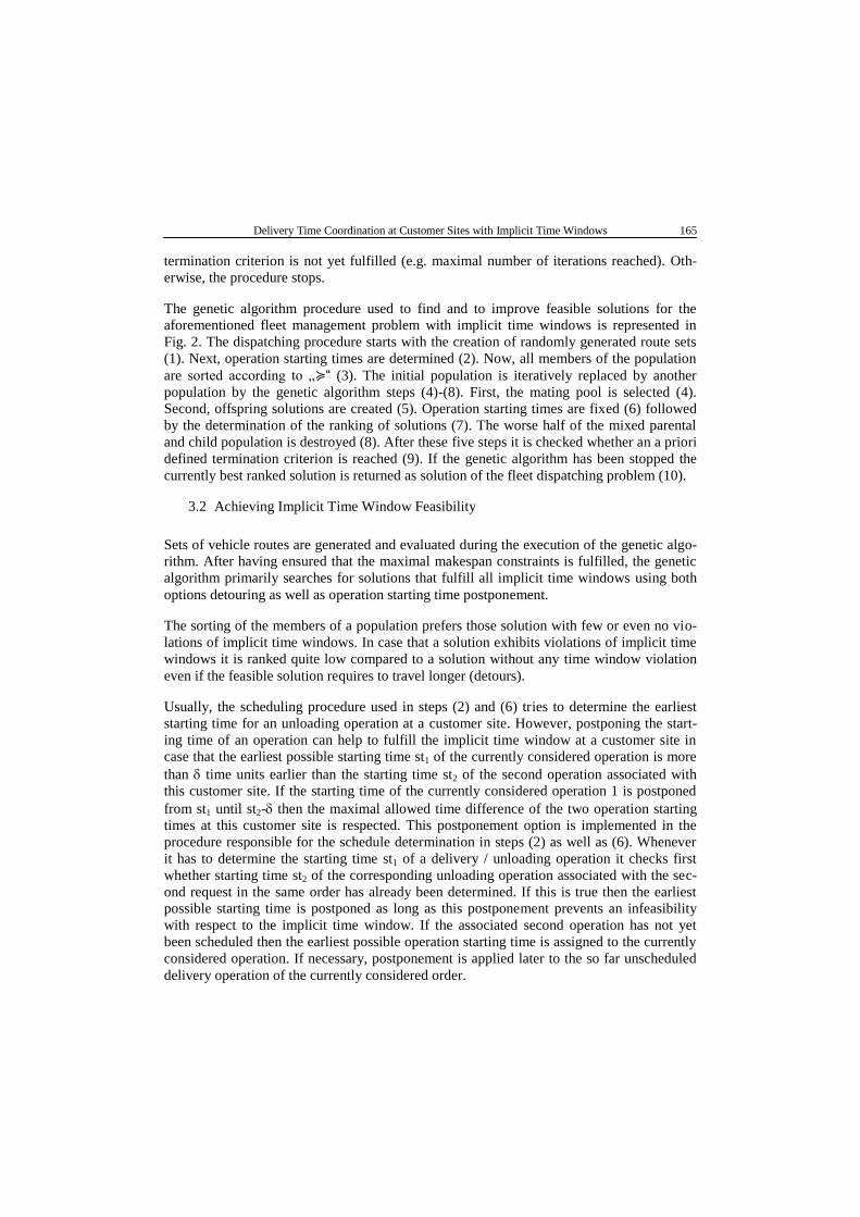
3.2 Achieving Implicit Time Window Feasibility

Sets of vehicle routes are generated and evaluated during the execution of the genetic algo-

rithm. After having ensured that the maximal makespan constraints is fulfilled, the genetic

algorithm primarily searches for solutions that fulfill all implicit time windows using both

options detouring as well as operation starting time postponement.

The sorting of the members of a population prefers those solution with few or even no vio-

lations of implicit time windows. In case that a solution exhibits violations of implicit time

windows it is ranked quite low compared to a solution without any time window violation

even if the feasible solution requires to travel longer (detours).

Usually, the scheduling procedure used in steps (2) and (6) tries to determine the earliest

starting time for an unloading operation at a customer site. However, postponing the start-

ing time of an operation can help to fulfill the implicit time window at a customer site in

case that the earliest possible starting time st1 of the currently considered operation is more

than time units earlier than the starting time st2 of the second operation associated with

this customer site. If the starting time of the currently considered operation 1 is postponed

from st1 until st2- then the maximal allowed time difference of the two operation starting

times at this customer site is respected. This postponement option is implemented in the

procedure responsible for the schedule determination in steps (2) as well as (6). Whenever

it has to determine the starting time st1 of a delivery / unloading operation it checks first

whether starting time st2 of the corresponding unloading operation associated with the sec-

ond request in the same order has already been determined. If this is true then the earliest

possible starting time is postponed as long as this postponement prevents an infeasibility

with respect to the implicit time window. If the associated second operation has not yet

been scheduled then the earliest possible operation starting time is assigned to the currently

considered operation. If necessary, postponement is applied later to the so far unscheduled

delivery operation of the currently considered order.


The schedule determining procedure employs a route-based schedule building strategy. It

determines the starting times of all operations for a first route. Then it determines the start-

ing times for all operations belonging to a second route and so on. With the goal to exploit

as much postponement opportunities as possible, we sort the routes by decreasing route

duration before we start we the determination of the schedules for the individual vehicles,

i.e. operations in the longest lasting route are scheduled prior to operations of shorter

routes.

4. Computational Experiments

This section reports about the specification, preparation, execution and evaluation of com-

putational experiments in which the aforementioned dispatching system is assessed. The

achieved results enable an estimation of additional costs as well as of other impacts of con-

sidering implicit time windows in vehicle route construction.

Subsection 4.1 addresses the specification of simulation scenarios. In Subsection 4.2 we

summarize the experimental setup, i.e. we outline the conducted experiments and introduce

the observed performance indicators. The presentation of the observed results as well as

their analysis are found in Subsection 4.3.

4.1 Specification of Test Scenarios

In order to conduct the announced computational simulation experiments we setup a collec-

tion of test scenarios. The subsequently outlined general setup applies for all these test

cases and comprises at fleet of 10 vehicles. This fleet comprises five type-A vehicles and

five type-B vehicles. The fleet operates in the area represented by the square [-300; 300] ×

[-300; 300]. Initially, all vehicles are positioned at the trucking company’s depot at point

(0;0). It is necessary that each vehicle finally returns to this location after it has completed

all assigned operations.

There are two warehouses available. Each warehouse stores one commodity exclusively.

Commodity A is stocked at warehouse WH-A which is located at (−150; 150). Commodity

B is stocked at warehouse WH-B located at (200;−50).

There are 25 orders. Each order comprises two origin-to-destination requests (od-requests).

Each od-request requires the pickup of a commodity quantity at the corresponding ware-

house and the delivery of this commodity to an individual customer site. The two od-

requests contained in an order fulfill the following two properties. First, their delivery loca-

tions coincide. Second, the first od-request requires the delivery of a type-A commodity but

the second od-request is associated with a type-B commodity. Consequently, each of the 25

customer sites must be visited twice: once by a type-A vehicle and once by a type-B vehi-

cle. We randomly draw five different sets of 25 customer locations using five different

random number generator seeding values ∈ ={1,…,5}.


The fleet dispatcher has to setup a set of routes with a least possible sum of total travelled

distance units for the fleet so that all 50 od-requests contained in the 25 orders are served.

We are going to analyze the impacts of varying the maximal allowed difference between

the two visits to be scheduled by the fleet dispatcher at each customer site (common length

of the implicit time window for all customer sites). Three different situations are distin-

guished. If =∞ then there is no coordination of the two visits necessary. Preliminary exper-

iments have revealed that arrival time difference larger than 500 time units are to be im-

plemented if the travel distance sum over all vehicle routes is minimal. In a second experi-

ment we therefore limit the maximal allowed unloading starting time difference at each

customer site to =500 time units. This enforces the fleet dispatcher to revise the least dis-

tance route set in order to fulfill the requirements of the implicit time windows of length

=500 time units at each customer site. Finally, in a third experiment, we want to analyze

the impacts of enforcing the two unloading operations to the same starting time (=0). In

total, we analyze the three implicit time window lengths :={∞;500;0}.

With the intention to keep the total travel distances as short as possible a fleet dispatcher

would preferentially apply a waiting strategy to achieve the implicit time window feasibil-

ity of the generated vehicle operation schedules. The insertion of waiting times at customer

sites contributes to the prolongation of the makespan, which is the time span between the

leaving of the first vehicle from the depot and the return of the last vehicle to the depot. The

specification of a maximal allowed makespan MSmax

implies that the fleet dispatcher has to

revise some routes in order to avoid any exceeding of MSmax

. In the aforementioned prelim-

inary experiments we have seen that the maximal makespan without any time-related op-

eration starting restriction is larger than 3000 time units. The reduction of MSmax

from (the

referential value) of ∞ time units to 3000 time units makes a route set revision become

necessary in order to comply with this the maximal allowed makespan. We investigate

scenarios with the maximal allowed makespan values MSmax:={∞;3000;2000}.

In summary, following the aforementioned ideas, we setup ||·||·|| = 5·3·3 = 45 different

fleet dispatching (vehicle routing) scenarios. For each of the 5 customer location sets we

can have 9 different time-oriented limitation sets by combining different maximal

makespan values with different values for the length of the implicit time windows at the

customer sites.

4.2 Setup of Experiments

In each individual simulation experiment, the genetic algorithm outlined in Section 3 is

used to mimic a dispatcher that determines a feasible schedule with least travel distances

for a given test case (;;MSmax

). The genetic algorithm is a randomized procedure so that

it is necessary to apply it with several random number seeding values to the same instance

in order to get a reliable average solution quality estimation. Here, each of the 45 test cases

is solved by the genetic algorithm with five different seeding values. This leads to

5·45=225 individual simulation experiments.


In all experiments, we observe several performance indicator values, store them and calcu-

late the average values for each combination (;MSmax

) of the length of the implicit time

window and the maximal allowed makespan MSmax

. The averagely observed travel distance

is stored in D(;MSmax

). Since we are interested in getting insights into the impacts of vary-

ing the length of the implicit time window, we calculate and store the relative increase

Dvar

(;MSmax

):= D(;MSmax

)/ D(∞;MSmax

) of the travel distance that results from the reduc-

tion of . Similarly, we store the average number of deployed vehicles in V(;MSmax

) and

its relative variation in Vvar

(;MSmax

). Furthermore, we save the average contribution of

waiting (idle) times to the total “away from the depot”-time of the deployed vehicles and

store this percentage in W(;MSmax

).

In order to identify structural changes of a route set implied by the reduction of the implicit

time window length it is necessary to compare routing as well as clustering decisions with

and without consideration of the implicit time windows at customer sites. We can quantify

the percentage of revised decisions using the H2-route set comparison measure proposed in

Schönberger (2015a). Let Kclust

(;MSmax

) denote the percentage of revised clustering deci-

sions (varied assignments of requests among vehicles) resulting from sharpening the length

of the implicit time window from ∞ to . In the same way, we define Kseq

(;MSmax

) to rep-

resent the percentage of the implied sequencing decision variations.

4.3 Presentation and Discussion of Results

Figure 3 shows the solution of an example instance with unlimited makespan and an im-

plicit time window of length =∞ generated by the genetic algorithm. Two vehicles are

deployed, one vehicle is of type A but the other one vehicle is of type B. The type B – vehi-

cle (route printed in gray) follows the route depot→ WH-B→ X→ W→ V→ U→ T→ S→

P→ Q→ R→ Y→ F→ E→ D→ A→ G→ H→ I→ J→ K→ L→ M→ N→ O→ B→ C→

depot. The type A – vehicle (route printed in black) travels along the route depot→ WH-

A→ A→ B→ C→ D→ E→ F→ G→ H→ I→ J→ K→ L→ M→ N→ O→ P→ Q→ R→

S→ T→ U→ V→ W→ X→ Y→ depot.


Figure 3: Routes generated for an instance with unlimited makespan and implicit time

window length =∞

Figure 4: Routes generated for the instance from Figure 3 with unlimited makespan

and implicit time window length =500


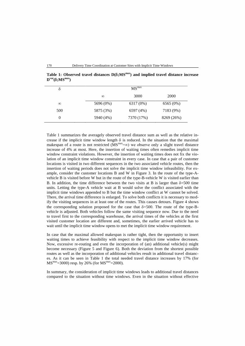
Table 1: Observed travel distances D(;MSmax

) and implied travel distance increase

Dvar

(;MSmax

)

MSmax

∞ 3000 2000

∞ 5696 (0%) 6317 (0%) 6565 (0%)

500 5875 (3%) 6597 (4%) 7183 (9%)

0 5940 (4%) 7370 (17%) 8269 (26%)

Table 1 summarizes the averagely observed travel distance sum as well as the relative in-

crease if the implicit time window length is reduced. In the situation that the maximal

makespan of a route is not restricted (MSmax

=∞) we observe only a slight travel distance

increase of 4% at most. Here, the insertion of waiting times often remedies implicit time

window constraint violations. However, the insertion of waiting times does not fix the vio-

lation of an implicit time window constraint in every case. In case that a pair of customer

locations is visited in two different sequences in the two associated vehicle routes, then the

insertion of waiting periods does not solve the implicit time window infeasibility. For ex-

ample, consider the customer locations B and W in Figure 3. In the route of the type-A-

vehicle B is visited before W but in the route of the type-B-vehicle W is visited earlier than

B. In addition, the time difference between the two visits at B is larger than =500 time

units. Letting the type-A vehicle wait at B would solve the conflict associated with the

implicit time windows appended to B but the time window conflict at W cannot be solved.

There, the arrival time difference is enlarged. To solve both conflicts it is necessary to mod-

ify the visiting sequences in at least one of the routes. This causes detours. Figure 4 shows

the corresponding solution proposed for the case that =500. The route of the type-B-

vehicle is adjusted. Both vehicles follow the same visiting sequence now. Due to the need

to travel first to the corresponding warehouse, the arrival times of the vehicles at the first

visited customer location are different and, sometimes, the earlier arrived vehicle has to

wait until the implicit time window opens to met the implicit time window requirement.

In case that the maximal allowed makespan is rather tight, then the opportunity to insert

waiting times to achieve feasibility with respect to the implicit time window decreases.

Now, excessive re-routing and even the incorporation of (an) additional vehicle(s) might

become necessary (Figure 5 and Figure 6). Both the deviation from the shortest possible

routes as well as the incorporation of additional vehicles result in additional travel distanc-

es. As it can be seen in Table 1 the total needed travel distance increases by 17% (for

MSmax

=3000) resp. by 26% (for MSmax

=2000).

In summary, the consideration of implicit time windows leads to additional travel distances

compared to the situation without time windows. Even in the situation without effective


maximal makespan, small travel distance increases are observed in order to meet the re-

quirements of an implicit time window since inserted waiting periods are insufficient to

achieve time window feasibility. If the maximal allowed makespan is rather short then

more than 25% of additional travel distances must be realized in order to fulfill the implicit

time windows.

Figure 5: Routes generated for an instance with maximal allowed makespan

MSmax

=2000 and unlimited implicit time window length =∞

Table 2: Averagely observed number of deployed vehicles V(;MSmax

) and implied

increase of needed vehicles Vvar

(;MSmax

)

MSmax

∞ 3000 2000

∞ 2 (0%) 3.52 (0%) 4.16 (0%)

500 2 (0%) 3.68 (5%) 4.64 (12%)

0 2 (0%) 3.92 (11%) 5.8 (39%)

A major driver of the additional travel distances is the increase of the number of additional-

ly needed vehicles to be deployed in order to meet the requirements of the implicit time


windows at the customer sites. Whenever a vehicle is deployed then additional travel dis-

tances for travelling back from the last customer occur. The values summarized in Table 2

show that the number of deployed vehicles can be kept stable only if the maximal allowed

makespan is large (MSmax

=∞). But as soon as the route duration is limited (MSmax

=3000)

then the sharpening of the time window length implies an increase of the number of aver-

agely deployed vehicles by up to 11%. If the maximal allowed makespan is quite tight

(MSmax

=2000) then even an increase of 39% of the number of incorporated vehicles is

reported.

Figure 6: Routes generated for an instance with maximal allowed makespan

MSmax

=2000 and unlimited implicit time window length =∞

Table 3: Contribution of waiting time W(;MSmax

)

MSmax

∞ 3000 2000

∞ 0% 0% 0%

500 0% 12% 5%

0 3% 9% 12%


The usage of inserting waiting times to synchronize the arrival times of both vehicles at

customer sites can be analyzed by means of the values compiled in Table 3. If the route

duration is unlimited then the routes are quite long and waiting periods are relatively short

so that these idle periods contribution to the total time until the return to the depot by 3% at

most. In case that MSmax

=3000 then the reduction of the length of the implicit time window

down to 500 time units requires additional waiting times and the contribution of these idle

times summarizes up to 12% contribution to the total operational time. A further reduction

of the implicit time window length implies the deployment of additional vehicles. Now, the

sum of waiting period lengths is reduced but detours (in form of additional travel distances

caused by the additionally incorporated vehicles) have to be implemented to meet the im-

plicit time window requirements. Only 9% of the total operational time is spent with wait-

ing. In case that MSmax

=2000 then the incorporation of additional vehicle does not avoid the

increase of idle times. Here, up to 12% of the time vehicles are away from the depot is

spent with waiting.

Table 4: Implied revision of clustering decisions Kclust

(;MSmax

)

MSmax

∞ 3000 2000

∞ 0% 0% 0%

500 0% 39% 56%

0 0% 44% 59%

With the goal to get additional insights and a better understanding of the impacts of sharp-

ened implicit time windows we compare (for a fixed maximal makespan value) the route

sets proposed with and without (=∞) implicit time windows. In particular, we analyze the

percentage of those pairs of requests that are served together in a common route without

implicit time window consideration but which are not served in one route in the route set

proposed for the situation with implicit time windows. Table 4 contains these percentage

values. If the route duration is unlimited (MSmax

=∞) then no revision of the clustering deci-

sion is necessary to comply with the implicit time windows. In case that an effective route

duration limitation is stated (MSmax

≤3000) then more than 39% of the pairs of clustered

requests are split as soon as ≤500. At maximum, 59% of these request pairs are split up.


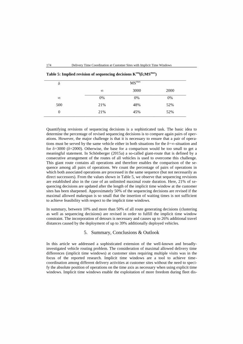
Table 5: Implied revision of sequencing decisions Kseq

(;MSmax

)

MSmax

∞ 3000 2000

∞ 0% 0% 0%

500 21% 48% 52%

0 21% 45% 52%

Quantifying revisions of sequencing decisions is a sophisticated task. The basic idea to

determine the percentage of revised sequencing decisions is to compare again pairs of oper-

ations. However, the major challenge is that it is necessary to ensure that a pair of opera-

tions must be served by the same vehicle either in both situations for the =∞-situation and

for =3000 (=2000). Otherwise, the base for a comparison would be too small to get a

meaningful statement. In Schönberger (2015a) a so-called giant-route that is defined by a

consecutive arrangement of the routes of all vehicles is used to overcome this challenge.

This giant route contains all operations and therefore enables the comparison of the se-

quence among all pairs of operations. We count the percentage of pairs of operations in

which both associated operations are processed in the same sequence (but not necessarily as

direct successors). From the values shown in Table 5, we observe that sequencing revisions

are established also in the case of an unlimited maximal route duration. Here, 21% of se-

quencing decisions are updated after the length of the implicit time window at the customer

sites has been sharpened. Approximately 50% of the sequencing decisions are revised if the

maximal allowed makespan is so small that the insertion of waiting times is not sufficient

to achieve feasibility with respect to the implicit time windows.

In summary, between 10% and more than 50% of all route generating decisions (clustering

as well as sequencing decisions) are revised in order to fulfill the implicit time window

constraint. The incorporation of detours is necessary and causes up to 26% additional travel

distances caused by the deployment of up to 39% additionally deployed vehicles.

5. Summary, Conclusions & Outlook

In this article we addressed a sophisticated extension of the well-known and broadly-

investigated vehicle routing problem. The consideration of maximal allowed delivery time

differences (implicit time windows) at customer sites requiring multiple visits was in the

focus of the reported research. Implicit time windows are a tool to achieve time-

coordination among different delivery activities at customer sites without the need to speci-

fy the absolute position of operations on the time axis as necessary when using explicit time

windows. Implicit time windows enable the exploitation of more freedom during fleet dis-


position. However, the management of implicit time windows in computer-supported au-

tomatic fleet disposition comes along with a lot of challenges.

The contribution of this article to the understanding and promotion of implicit time win-

dows is two folded. First, we have proposed a prototypic automatic scheduling system that

is able to handle implicit time windows by inserting waiting times as well as detours to

enforce coupled operation starting times in the implicit time window. Second, we have used

this tool to conduct simulation experiments in which we observed the impacts of consider-

ing implicit time windows during fleet disposition. These contributions answer the research

questions stated in the introduction of this research report.

The introduction and/or the sharpening of implicit time windows require the revision of

routing decisions. Implicit time windows help to offer logistics service providers a better

and more appropriate service level. The interface performance between (external) transport

processes and (internal) downstream processes in a value chain benefits from implicit time

windows. However, we have seen that a significant increase of travel distances comes along

with the consideration of implicit time windows. Furthermore, more vehicles are necessary

to meet implicit time window requirements in time sensitive distribution scenarios.

Although we have already achieved first insights into the benefits and drawbacks of using

implicit time windows in distribution logistics further research is necessary to get a deeper

understanding of this coordination tool. Especially, it is necessary to investigate setups in

which implicit time windows are customized, i.e. each customer defines the length of its

implicit time window individually. Second, limited vehicle as well as limited handling

capacities must be integrated into the fleet disposition system. Third, other objectives guid-

ing the vehicle scheduling process require an assessment. In this context, a total cost calcu-

lation is necessary in order to estimate the surcharge a customer has to pay for being served

in a shorter implicit time window. In addition, the optimization of emissions resulting from

the transport operations should be assessed in the context of implicit time windows.

6. Abstract

Enterprises as well as private households exploit multi-sourcing strategies that lead to

fragmented material flows and multiple deliveries. Often, customer (unloading) sites are

visited several times by different vehicles of a transport service provider. In order to avoid

costly setup at business customer sites and with the goal to increase the probability to meet

a private customer in a first delivery attempt it is necessary to coordinate the multiple visits.

In this context moveable time windows (also called implicit time windows) are proposed as

coordination tool. In contrast to explicit time windows, a moveable time window does not

restrict the customer visiting time to a certain part of the time axis but it only limits the time

differences among the necessary unloading operations at a certain customer site. The prima-

ry goal of the here reported research comprises the evaluation of impacts on least distance

vehicle routes and on the number of required vehicles implied by the consideration of im-


plicit time windows from the perspective of a carrier company. We report about simulation

experiments.

Multisourcing-Stragien von Unternehmen und Privathaushalten führen zu einer Fragmen-

tierung von Transporten und Anlieferungsvorgängen im Wareneingang bzw. bei der Sen-

dungsaushändigung. Häufig werden dadurch mehrfache Besuche eines Kunden durch ver-

schiedene Fahrzeuge (eines Transportdienstleisters) notwendig. Zur Vermeidung von Um-

rüstaufwendungen bzw. zur Erhöhung der Wahrscheinlichkeit einer erfolgreichen Sen-

dungsaushändigung ist eine zeitliche Abstimmung der Anlieferungen an Auslieferungsorten

notwendig. In dieser Arbeit werden variable bzw. bewegliche Zeitfenster (sog. implizite

Zeitfenster) als Koordinationsmechanismus vorgeschlagen und aus der Sicht eines Straßen-

güterverkehrsunternehmens evaluiert. Im Gegensatz zu explizit definierten Zeitfenstern

wird der Belieferungszeitpunkt nicht vorab eingeschränkt sondern lediglich der Abstand

zwischen den einzelnen Anlieferungen nach oben beschränkt. Das übergeordnete Ziel der

hier berichteten Forschungsarbeiten umfasst die Abschätzung von Auswirkungen verschie-

dener Konfigurationen von impliziten Zeitfenstern. Anhand der in Simulationsexperimen-

ten beobachteten streckenminimalen Transportprozesse werden die Auswirkungen ver-

schiedener Konfigurationen von impliziten Zeitfenstern auf Fahrtrouten und benötigte

Fahrzeuge abgeschätzt.

7. References

Agrawal, N., Smith, S.A., Tsay, A.A., 2002. Multi-Vendor Sourcing in A Retail Supply

Chain. Production and Operations Management 11(2), 157-182

Archetti, C., Campbell, A., Speranza, M. G., 2014. Multicommodity vs. Single-Commodity

Routing. Transportation Science (to appear).

Archetti, C., Speranza, M. G., 2008. The split delivery vehicle routing problem: A survey.

In: Golden, B., Raghavan, S., Wasil, E. (Eds.), The Vehicle Routing Problem: Latest Ad-

vances and New Challenges. Springer, New York, 103– 122.

Breier, H., 2015. Tourenplanung mit alternativen Lieferperioden und Teillieferungen. KIT

Scientific Publishing, Karlsruhe.

Cattanuzza, D., Absi, N., Feillet, D., Vidal, T., 2014. A memetic algorithm for the multi trip

vehicle routing problem. European Journal of Operational Research 236, 833–848.

Clausen, T., 2011. Airport Ground Staff Scheduling. DTU Management Engineering, PhD

Thesis.

Crainic, T.G., Laporte, G. (Eds.), 1998. Fleet Management and Logistics. Springer, New

York


Crevier, B., Cordeau, J.-F., Laporte, G., 2007. The multi-depot vehicle routing problem

with inter-depot routes. European Journal of Operational research 176, 756–773.

de Jong, C., Kant, G., van Vliet, A., 1996. On Finding Minimal Route Duration in the Ve-

hicle Routing Problem with Multiple Time Windows. Utrecht University, Technical Report

TR-120-96.

Doerner, K.F., Gronalt, M., Hartl. R.F., Kiechle, G., Reimann, M., 2008. Exact and heuris-

tic algorithms for the vehicle routing problem with multiple interdependent time windows.

Computers & Operations Research 35, 3034 – 3048.

Drexl, M., 2012. Synchronization in vehicle routing—a survey of vrps with multiple syn-

chronization constraints. Transportation Science 46(3), 297–316.

Favaretto, D., Moretti, E., Pellegrini, P., 2007. Ant colony system for a vrp with multiple

time windows and multiple visits. Journal of Interdisciplinary Mathematics 10 (2), 263–

284.

Goel, A., Meisel, F., 2013. Workforce routing and scheduling for electricity network

maintenance with downtime minimization. European Journal of Operational Research 231,

210–228.

Golden, B., Raghavan, S., Wasil, E. (Eds.), 2008. The Vehicle Routing Problem: Latest

Advances and New Challenges. Springer, New York.

Parragh, S., Doerner, K., Hartl, R., 2008. A survey on pickup and delivery problems. Jour-

nal für Betriebswirtschaft 58, 21–51.

Schönberger, J., 2015. The two-commodity capacitated vehicle routing problem with syn-

chronization. IFAC-PapersOnLine 48 (3), 168 – 173, 15th IFAC Symposium on Infor-

mation Control Problems in Manufacturing (INCOM 2015)

Schönberger, J., 2015a. Computing Indicators for Differences and Similarities among Sets

of Vehicle Routes. Technical Report. Chair of Transport Services and Logistics, TU Dres-

den.

Schönberger, J., 2011. Model-Based Control of Logistics Processes in Volatile Environ-

ments. Springer New York.

Solomon, M. M., 1987. Algorithms for the vehicle routing and scheduling problems with

time window constraints. Operations Research 35 (2), 254–265.

Stieber, A., Yuan, Z., Fügenschuh, A., 2015. School Taxi Routing for Children with Spe-

cial Needs. Universität der Bundeswehr Hamburg, Technical Report AMOS#19(2015).


Vidal, T., Crainic, T., Gendreau, M., Lahrichi, N., Rei, W., 2012. A hybrid genetic algo-

rithm for multidepot and periodic vehicle routing problems. Operations Research 60(3),

611–624.

Documents

Delivery Time Coordination at Customer Sites with Implicit ...z-f-v.de/fileadmin/archiv/hefte---2015_1_2_3/2015-2/ZfV_2015_Heft_2_03...156 Delivery Time Coordination at Customer Sites