Demagnetizing factors for cylinders - Purdue University

IEEE TRANSACTIONS ON MAGNETICS, VOL. 21, NO. 4, JULY 1991 3601

Demagnetizing Factors for Cylinders Du-Xing Chen, James A. Brug, Member, IEEE, and Ronald B. Goldfarb, Senior Member, IEEE

Abstract-Fluxmetric (ballistic) and magnetometric demagnetizing factors Nf and N , for cylinders as functions of susceptibility x and the ratio y of length to diameter have been evaluated. Using a one-dimensional model when y 2 10, Nf was calculated for - 1 5 x < Q) and N,,, was calculated for x + 00.

Using a two-dimensional model when 0.01 5 y 5 50, an important range for magnetometer measurements, N , and Nf were calculated for -1 5 x < 00. Demagnetizing factors for x < 0 are applicable to superconductors. For x = 0, suitable for weakly magnetic or saturated ferromagnetic materials, Nf and N,,, were computed exactly using inductance formulas.

I. INTRODUCTION HE study of demagnetizing factors for ellipsoids and T their degenerate forms (spheres, infinite plates, infi-

nite cylinders) dates from the work of Poisson [ 11 and was elaborated upon by Thomson [2], Evans and Smith [3], and Maxwell [4]. Experimental investigations on finite right circular cylinders began in the 1870’s, when ballistic galvanometers were first used in magnetic measurements of iron [5], [6]. The literature distinguishes between “magnetometric” and “fluxmetric” (or “ballistic”) demagnetizing factors N , and Nf [7]. N , refers to an average of magnetization over the entire specimen and is appropriate for magnetometer measurements of small samples. Nf refers to an average of magnetization at the midplane of the sample and is appropriate for measurements made with short search coils. Values of the demagnetizing factor were deduced from the shearing of the magnetic hysteresis loop [8], a procedure originally developed by Lord Rayleigh for ellipsoids [9], or by measuring the magnetization and the field at the cylinder’s side [ 101. Factors for cylinders of several aspect ratios were published [7], [8], [ l l ] , [12]. By the 1900’s, it was apparent that the values of the factors depended on the susceptibility x of the material [13]-[15].

Although it has been criticized from a pedagogical point of view [16], [17], the use of fictitious magnetic poles to calculate demagnetizing fields has been universal. The first theoretical treatment of magnetic pole distributions in finite cylinders was by Green [18]. An early model to attempt to explain experimental data considered point

Manuscript received March I I , 199 1, The authors are with the Electromagnetic Technology Division, National

D.-X. Chen is on leave from the Electromagnetism Group, Physics De-

J . A. Brug is on leave from the Thin Film Department, Hewlett-Packard

IEEE Log Number 9102083.

Institute of Standards and Technology, Boulder, CO 80303.

partment, Universitat Autbnoma de Barcelona, 08 I93 Bellaterra, Spain.

Laboratories, Palo Alto, CA 94303.

magnetic poles at each end of a cylinder [ 191. This sim- plistic model could be used only for long uniformly magnetized cylinders, and the results deviated significantly from experimental data on ferromagnetic samples. During the 1920’s and 1930’s, there were several theoretical papers on Nf for material with constant susceptibility x. The results were given as functions of x and the length-to- diameter ratio y. These used one-dimensional models with approximations as needed to suit the computational techniques of the time. The first systematic theoretical calculation of N’ for the high susceptibility case was done by Wurschmidt [20], [21]. He calculated Nf of cylinders using a one-dimensional model in which the cylinder had side surface poles and point end poles. He used Taylor expansions for the magnetization and the demagnetizing field at the midplane. The calculation was complicated, and he completed it only for the case y = 50 and x --+ W. For the y and x dependence of Nf, he gave qualitative results using the first few terms of the expansion. A similar approach with simpler expressions was used by Neu- mann and Warmuth [22], who calculated Nf for x + 00

a n d y 2 10. To obtain the susceptibility dependence of Nf, Stablein

and Schlechtweg [23] used a quadratic approximation and two linear differential equations. The model was im- proved by substituting uniform end-surface poles for point end poles. Their results included 30 values of Nf for 10 I y 5 500 and 12.56 I x c W. An extension of the y region to 0 was achieved by Warmuth [24]-[26], who fit- ted existing data and extrapolated graphically using the demagnetizing factor N of ellipsoids as a reference. The values of Nf calculated from the one-dimensional models were consistent with the data of ballistic measurements on soft magnetic materials. Bozorth and Chapin [27] com- piled the results, which were later plotted in Bozorth’s book [28].

To obtain axial demagnetizing factors more accurately, especially for short cylinders, two-dimensional calculations are needed. The simplest case is x = 0, where N , and Nf as functions of y can be derived analytically. The approximation x = 0 applies to diamagnets, paramagnets, and saturated ferromagnets. N,,, for 25 values of y from 0.2 to 1000 were obtained accurately to four significant figures by Brown [29] from a calculation of self-inductance [30] and listed as a table in Brown’s book [31]. Crabtree [32] obtained the same values for the average demagnetizing factor by integration of the local field over the cylindrical volume. Moskowitz et al. extended

U.S . Government work not protected by U.S. Copyright

1.- i-r

3602 IEEE TRANSACTIONS ON MAGNETICS, VOL. 27, NO. 4, JULY 1991

Brown’s method to cylinders of polygonal cross section [33], and KaczCr and Klem extended it to hollow cylinders [34]. Nf for x = 0 was calculated exactly by Joseph [35]. Approximate values for N , and Nf for x = 0, accurate for large y, were calculated by Vallabh Sharma using uniformly magnetized volume elements [36]. Sato and Ishii [37] obtained a simple expression to approximate N , for x = 0. Chen and Li [38], [39] obtained Nf for x = 0 using magnetostatic potential calculations.

The susceptibilities x = - 1 and x -+ 00 correspond to perfectly diamagnetic and ideally soft ferromagnetic materials, respectively. N , and Nf for these susceptibilities were first treated by Taylor for perfectly conducting cylinders [40], [41]. He developed a method introduced by Smythe that expressed charge densities on the side and ends in terms of a set of orthogonal polynomials, and expanded the electrostatic potential at the cylinder center [42]-[44]. Taylor calculated electric and magnetic polarizabilities for conducting cylinders for 0.25 I y 5 4 in both the longitudinal and transverse directions. N,(m) can be deduced from his electric polarizability results because of the analogy between electrostatics and magnetostatics. Because his calculation for magnetic polarizability was for a uniform quasi-static but nonpenetrating applied field, N,( - 1) can also be deduced from his results. According to Taylor, his convergence error was less than 0.1 % for the longitudinal direction.

Using a similar approach with simpler base functions, Templeton et al. calculated axial Nf for x -+ 03 for 0.05 I y I 250 [45], [46]. The fact that the side and end- pole densities have basically a 6- ’13 dependence, where 6 is the distance from the corner, was used to construct the set of polynomials. To estimate their error, Templeton and Arrott calculated the root-mean-square deviation of the normalized potential from 0 and found it to be less than 0.3 1 % [45]. Compared to an approximate formula with 8 adjustable parameters, the deviations of their 12 computed Nf(oo) values were less than 0.25 %. The work was based on their earlier magnetostatic analysis of the magnetization process in soft ferromagnetic cylinders with constant end-pole densities [47], [48]. The details of the calculation were published by Aharoni. who also calculated the self-energy of cylinders [49], and more gener- ally, cylinders with nonuniform magnetization [50].

For susceptibilities other than 0, - 1, and 00, different techniques have been used. Archer and Guancial [5 11 and Fawzi et al. [52] calculated the distribution of magnetization and magnetic field in long cylinders with large susceptibilities using volume and boundary integral equations. Using experimental resistance network analogs, Okoshi [53] obtained Nf for x -, 00, and Yamamoto and Yamada [54] obtained Nf and N,,, for large x.

Several papers have treated demagnetizing factors at points. Joseph and Schlomann [55] solved for local demagnetizing factors in uniformly magnetized cylinders and used a series expansion to account for nonuniform magnetization. Kraus [56] determined the complete local demagnetizing tensor for uniformly magnetized cylin-

ders. Brug and Wolf [57] calculated the magnetization distribution in disks and obtained the local demagnetizing factor for materials that undergo phase transitions.

In Zijlstra’s book [58], Nf and N , are plotted. These types of graphs and tables appear in other books on magnetism and magnetic materials, and they are widely used, sometimes inappropriately, in magnetic measurements of ferromagnetic, ferrimagnetic, weakly magnetic, and superconducting materials. However, there remain some problems. For x = 0, the most accurate case, the number of y values for N , and Nf is insufficient for accurate interpolation. For x # 0, almost all books give results obtained before 1950, and there are no data for x < 0. For long cylinders (y > lo), there is a lack of data on the x dependence of Nf, and there are no data on N,. For short cylinders (y < lo), there are even less data, and those that exist have large errors because they were obtained by extrapolation. In summary, there is no complete picture for the y and x dependence of Nf and N,.

In this paper, we calculate Nf and N , for a complete range of y and x. Susceptibility x is traditionally assumed to be constant in the material and is therefore defined as M / H , where M is the magnetic moment per unit volume and H is the internal magnetic field. For the case x = 0, in which the magnetization is uniform, we give 61 exact inductance calculations of N , and Nf for lop5 I y 5 lo3. For x # 0, more elaborate methods are used. For y > 10, the variation of magnetization across the radius of the cylinder is negligible at the midplane, and we calculate Nf as a function of y and x (- 1 I x < 00) based on the one-dimensional model of Stablein and Schlechtweg [23]. Unlike them, we use Taylor expansions for M ( z ) , calculate the demagnetizing field H d ( z ) directly at 25 points along the axis, and obtain more accurate results. The model is also applicable to N , for x -, 00. For 0.01 I y I 50, a two-dimensional finite element method is used that takes into account the variation of magnetic pole density along the side and ends of the cylinder. Values of N , and Nf are given for -1 I x < 00.

11. FLUXMETRIC AND MAGNETOMETRIC DEMAGNETIZING FACTORS

The demagnetizing correction is nontrivial for samples in open magnetic circuits. An exact correction can be obtained only for ellipsoids [4], [59], [60], where both the magnetization M and the demagnetizing field Hd are uniform under a uniform applied field H,. If the three principal ellipsoid axes coincide with the x , y , and z axes, the internal field is

H = H , + Hd = H, - N M , (1)

where N is the demagnetizing tensor,

I II I

CHEN et al.: DEMAGNETIZING FACTORS FOR CYLINDERS 3603

with

N, + N,, + Nz = 1. (2b) If the applied field is along one of the principal axes, we have

H = Ha + Hd = H , - N M , (3) where N is called the demagnetizing factor. In SI units, 0 5 N I 1. In cylindrical samples, which are commonly used in magnetic measurements, the demagnetizing field is not uniform, and two kinds of susceptibility-dependent demagnetizing factors are defined.

If the sample is located in a uniform applied field Ha along its axis, the fluxmetric (or ballistic) demagnetizing factor Nf is defined as the ratio of the average demagnetizing field to the average magnetization at the midplane perpendicular to the axis. The magnetometric demagnetizing factor N , is defined as the ratio of the average demagnetizing field to the average magnetization of the entire sample [58]:

(4)

Nf and N , are functions of the ratio y of cylinder length to diameter and the susceptibility x of the material. For ferromagnetic or ferrimagnetic materials, this x should be regarded as an effective x , similar to the differential susceptibility dM/dH at the corresponding magnetic state. In [58], the definition of N , is limited to x = 0.

111. N , AND Nf FOR x = 0 DETERMINED BY INDUCTANCE CALCULATIONS

Brown [29] showed how N , could be determined using a self-inductance calculation in which a uniformly magnetized cylinder was modeled as a solenoid. In fact, both N , and Nf may be calculated using the mutual inductance of two model solenoids of the same diameter. N , is obtained when the solenoids have the same length, and the problem reduces to the self-inductance calculation. Nf is obtained when the length of one of the model solenoids approaches 0, and the problem is that of the mutual inductance of a solenoid and a single-turn loop located at its midplane. In this section we calculate exact values of N , and Nffor x = 0 and a wide range of y.

A. Formulas for Inductance

An exact formula for the self-inductance L, of a thin solenoid of length 21, radius a, and number of turns n is [611

* [12F(k,) + (a2 - 12)E(k,)] - a 3 } , (6)

where F(k,) and E(k,) are the complete elliptic integrals of the first and second kind of modulus k,, which is defined by

(7) and po is the permeability of vacuum.

An exact formula for the mutual inductance L, of the same thin solenoid and a coaxial single-turn loop of the same radius at its midplane is [62]

(8)

(9)

Cohen [63] derived an exact general formula for the mutual inductance of two concentric coaxial thin solenoids (denoted by subscripts 1 and 2). We have used it successfully for these calculations, as an alternative to (6) and (8), with a2 = a l , in the limits l2 = I , (for N,) and l2 -+ 0 (for N f ) .

B. Relationship between N , and L,, Nf and L, The flux density B in a magnetic material is related to

the internal field H and the magnetization M : B = pO(H + M ) , where H is, in general, related to the applied and demagnetizing fields as defined for ellipsoids in (1). Thus B = po(Ha + Hd + M ) . Following Brown [29], we define B' as the Amperian flux density:

k: = a 2 / ( a 2 + Z 2 ) ,

Lm = (pOna/krn> [F(krn) - E(km)I,

k i = 4a2/(4a2 + 1 2 ) .

where the modulus k, is defined by

B' = B - poHa = po(Hd + M ) . (10)

When x = 0, a cylinder in an axial field has a uniform magnetization M . An ideal thin solenoid carrying current I through n turns over a length 21 is equivalent, with re- spect to the B' field, to a longitudinally magnetized cylinder coincident with it [29]. Thus the cylinder can be modeled as a solenoid with the same M , and its average Hd can be obtained from M and average B' using (10). We take the solenoid as having one turn (n = l ) , so

(1 1) M = I/(2l).

For the entire volume, we can obtain the average B' from the average flux 9 in the solenoid as

( B ' ) = +/(m2). ( 1 2 4

Thus the average demagnetizing field can be obtained from (10) and (12a) as

( H d ) = + / ( p ~ n a * ) - M . (1 3 4

L, = +/I . (144

The definition of self-inductance is

From ( l l ) , (13a), and (14a), we obtain the final expression forthe magnetometric demagnetizing factor:

N , - ( H d ) / M = 1 - 2&/(pona2). (15)

For N f , we obtain the average B' at the midplane from the flux a0 in the one-turn secondary loop of radius a:

( B ' ) = +0/(na2). ( 12b)


The average demagnetizing field is

( H d ) = *o/ (pona2) - M. (13b)

L, = *o/z. (14b)

The definition of mutual inductance is

The final expression for the fluxmetric demagnetizing factor is

Nf - (&)/A4 = 1 - 21L,/(po~a*). (16)

Equations (15) and (16) have been derived, by direct integration rather than inductance formulas,' by Joseph [35].

C. Results Values of N,(x = 0) and Nf(x = 0) as functions of y

(= Z/a) computed using (6), (15), (8), and (16) are given in Table I. For N,, the data agree with those given by Brown [29], [31]. For Nf, the data agree with those obtained by Joseph [35] and by Chen and Li [38]. In Table I we also give N for ellipsoids of revolution with longitudinal axes 21 and transverse axes 2a calculated from well-known formulas [4], [59], [60].

IV. ONE-DIMENSIONAL MODEL FOR LONG CYLINDERS A. Calculation of M

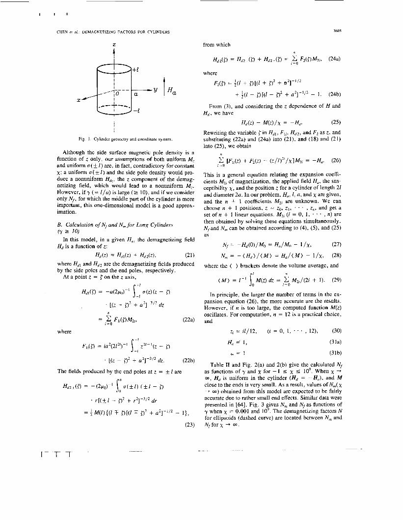
Assume that a cylinder of length 21 and diameter 2a is located in a uniform applied field Ha along the z axis, as shown in Fig. 1. The material has constant susceptibility x, which leads to

B = po(M + H) = poM(1 + l / x ) (17) at any point inside the cylinder. Since V * B = 0, the volume magnetic pole density, proportional to V - M, equals 0 inside the cylinder; that is, all poles are on the surface. <.''

We further assume for this one-dimensional model that M,, the z component of M, is uniform in each cross section of the cylinder, and can be expressed by a scalar quantity as

n

M(z) = M,(z) = c M2,(Z/O2', (18)

, n) are constants. (B , Ha, and

r = O

where M2,(i = 0, 1, Hd can also be written as scalar quantities.)

.

For a section of cylinder of length dz at z ,

$ M ds = na2dM(z) + 2aaMr(z)dz = 0, (19a)

because $ M - ds = V * M d v and V * M = 0. M r ( z ) is the radial component of M at the side surface. Substi- tuting a ( z ) = p o M r ( z ) gives, on the side surface, the surface magnetic pole density

U ( Z ) = -;poa dM(z) /dz = - ( p o a / l )

n

i M 2 1 ( ~ / l ) 2 r - ' .

(19b)

TABLE 1 EXACT FLUXMETRIC AND MAGNETOMETRIC DEMAGNETIZING FACTORS Nf

AND N,,, FOR x = 0"

Y N A O ) Nf (0) N ~~

0.00001 0.o001 0.001 0.01 0.02 0.03 0.04 0.05 0.06 0.07 0.08 0.09 0.10 0.12 0.14 0.16 0.18 0.20 0.22 0.24 0.26 0.28 0.30 0.32 0.34 0.36 0.38 0.40 0.45 0.50 0.55 0.60 0.65 0.70 0.75 0.80 0.90 1 .o 1.1 1.2 1.3 1.4 1.6 1.8 2.0 2.5 3 .O 3.5 4 5 6 7 8 9 10 20 50 100 200 500 lo00

0.9999 0.9994 0.9950 0.9650 0.9389 0.9161 0.8954 0.8764 0.8586 0.8419 0.8261 0.8110 0.7967 0.7698 0.7450 0.7219 0.7004 0.6802 0.661 1 0.6432 0.6262 0.6101 0.5947 0.5801 0.5662 0.5530 0.5403 0.5281 0.4999 0.4745 0.4514 0.4303 0.41 10 0.3933 0.3770 0.3619 0.3349 0.3116 0.291 1 0.2731 0.2572 0.2429 0.2186 0.1986 0.1819 0.1501 0.1278 0.1112 0.09835 0.07991 0.06728 0.05 809 0.05110 0.04562 0.041 19 0.0209 1 0.00843 8 0.004232 0.002119 0.0008483 0.0004243

0.9999 0.9993 0.9949 0.9638 0.9364 0.9124 0.8905 0.8703 0.8513 0.8333 0.8163 0.8001 0.7845 0.7553 0.7281 0.7027 0.6789 0.6565 0.6352 0.6151 0.5960 0.5778 0.5604 0.5438 0.5279 0.5127 0.4982 0.4842 0.4516 0.4221 0.3952 0.3705 0.3480 0.3273 0.3082 0.2905 0.2592 0.2322 0.2089 0.1886 0.1710 0.1555 0.1298 0.1096 0.09351 0.06544 0.04799 0.03653 0.02865 0.01889 0.01334 0.009904 0.007635 O.Oo6061 0.004927 0.001245 0.0001999 0.00004999 O.oooO1250 0.00000200 0.00000050

1 .m 0.9998 0.9984 0.9845 0.9694 0.9546 0.9402 0.9262 0.9125 0.8991 0.8860 0.8733 0.8608 0.8367 0.8137 0.7917 0.7706 0.7505 0.7312 0.7126 0.6948 0.6778 0.6614 0.6456 0.6304 0.6158 0.6017 0.5b82 0.5563 0.5272 0.5005 0.4758 0.4531 0.4321 0.4126 0.3944 0.3618 0.3333 0.3083 0.2861 0.2664 0.2488 0.2187 0.1941 0.1736 0.1351 0.1087 0.08965 0.0754 1 0.05 582 0.04323 0.03461 0.02842 0.02382 0.02029 0.006749 0.001443 0.0004299 0.0001248 0.00002363 O.OOOOO6601

'Factors were calculated as functions of y using inductance formulas. For comparison, N is the demagnetizing factor for ellipsoids.

On the end planes of the cylinder, we have uniform surface magnetic pole densities:

n

r = O U(* 1 ) = k p o ~ ( l ) = 5 PO ,E ~ 2 i . (20)

ndilley

Comment on Text

I think they mean gamma = L/(2a)

I II ' I

CHEN et al. : DEMAGNETIZING FACTORS FOR CYLINDERS 3605

z

-I----

X uy -'-?--'- -e I H a I

Fig. 1. Cylinder geometry and coordinate system.

Although the side surface magnetic pole density is a function of z only, our assumptions of both uniform M, and uniform a( k I) are, in fact, contradictory for constant x; a uniform a +_ 1) and the side pole density would produce a nonuniform Hdzr the z component of the demagnetizing field, which would lead to a nonuniform M,. However, if y (= l / a ) is large ( 2 lo), and if we consider only Nf, for which the middle part of the cylinder is more impoltant , this one-dimensional model is a good approximation.

B. Calculation of Nf and N,,, for Long Cylinders (7 1 10)

Hd is a function of z : In this model, in a given Ha, the demagnetizing field

H d ( z ) = Hdl(z) + Hd2(z), (21) where Hdl and Hd2 are the demagnetizing fields produced by the side poles and the end poles, respectively.

At a point z = {on the z axis, +I

HdI({) = -a(2/h)-' fl(z>(z - - I

[ ( z - {)2 + a2Ip3/* dz

where P +I

where

F2(33 = ;(I + {)[(l + { ) 2 + t12]-1/2

+ i ( l - { ) [ ( t - {)2 + a2]- ' /2 - 1. (24b)

From (3), and considering the z dependence of H and

(25)

Rewriting the variable {in H d l , F I I , H d 2 , and F2 as z , and substituting (22a) and (24a) into (21), and (18) and (21) into (25), we obtain

H d , we have

H ~ ( z ) - M(z)/x = -Ha.

n

c [F,,(z) + F2(z) - (z/l)21/XlM21 = -Ha. (26) r = O

This is a general equation relating the expansion coefficients M2r of magnetization, the applied field H,, the susceptibility x , and the position z for a cylinder of length 21 and diameter 2a. In our problem, H,, I, a, and x are given, and the n + 1 coefficients M,, are unknown. We can choose n + 1 positions, z = zO, zI, * * * , z,, and get a set of n + 1 linear equations. M2, (i = 0, 1, - * , n ) are then obtained by solving these equations simultaneously. Nf and N,,, can be obtained according to (4), (5), and (25) as

Nf = -Hd(o)/MO = Ha/MO - l /X, (27)

N , = - ( H d ) / ( M ) = H a / ( M ) - l / x , (28)

where the ( ) brackets denote the volume average, and n

( M ) = I - ' M(z) dz = c M2,/(2i + 1). (29)

In principle, the larger the number of terms in the expansion equation (26), the more accurate are the results. However, if n is too large, the computed function M ( z ) oscillates. For computation, n = 12 is a practical choice, and

s: 1 = O

z, = if / l2, (30)

H, = 1, (314

r c = ! (3 1b)

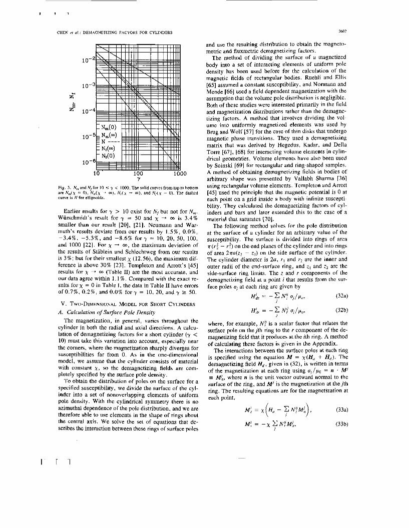
Table I1 and Fig. 2(a) and 2(b) give the calculated Nf as functions of y and 2 for -1 I x I lo9. When x +

03, Hd is uniform in the cylinder (Hd = - H a ) , and M close to the ends is very small. As a result, values of N,( x -+ 00) obtained from this model are expected to be fairly accurate due to rather small end effects. Similar data were presented in 1641. Fig. 3 gives N , and Nf as functions of y when x = 0.001 and lo9. The demagnetizing factors N for ellipsoids (dashed curve) are located between N,,, and Nf for x -+ 00.

(i = 0, 1, * * * 9 121,


TABLE I1 N, AS FUNCTION OF y A N D x CALCULATED USING THE ONE-DIMENSIONAL MODEL'

Y 1000 2000 10 20 50 100 200 500

N/ X (IO-)) ( IO- ) ) IO-^) (IO-') (IO-') (10-7 (IO-') (IO-')

- 1 3.965 1.130 1.900 4.776 1.196 1.917 4.796 1.199 -0.8 4.239 1.162 1.931 4.852 1.215 1.945 4.865 1.216 -0.4 4.642 1.210 1.972 4.944 1.237 1.980 4.950 1.237

0 4.963 1.248 1.999 5.000 1.250 2.000 5.000 1.250 0. I 5.037 1.256 2.005 5.011 1.252 2.004 5.010 1.252 0.2 5.108 1.265 2.011 5.021 1.255 2.007 5.018 1.255 0.5 5.315 1.289 2.026 5.047 1.260 2.016 5.040 1.260 1 5.639 1.328 2.049 5.082 1.268 2.027 5.067 1.267 2 6.231 1.401 2.089 5.135 1.277 2.040 5.100 1.275 5 7.695 1.616 2.191 5.247 1.293 2.058 5.143 1.286 10 9.377 1.967 2.352 5.394 1.308 2.071 5.168 1.292 20 11.23 2.565 2.688 5.664 1.332 2.083 5.187 1.296 so 13.21 3.600 3.803 6.494 1.395 2.106 5.211 1.299 100 14.14 4.294 5.448 8.132 1.500 2.141 5.238 1.302 200 14.68 4.776 7.497 11.77 1.734 2.210 5.288 1.305 500 15.03 5.126 9.800 19.91 2.661 2.414 5.438 1.316

IO3 15.15 5.255 10.90 26.32 4.221 2.808 5.684 1.333 2 X IO3 15.21 5.322 11.53 31.12 6.275 3.889 6.186 1.369 5 X IO3 15.25 5.363 11.95 34.78 8.642 7.570 8.223 1.474

IO4 15.26 5.377 12.09 36.16 9.779 11.68 13.12 1.669 2 X IO4 15.27 5.384 12.16 36.88 10.44 15.47 22.71 2.237 5 X IO4 15.27 5.388 12.21 37.33 10.87 18.77 38.36 4.620

IO5 15.27 5.390 12.22 37.48 11.02 20.11 47.73 7.811 2 X IO5 15.28 5.390 12.23 37.55 11.10 20.83 53.77 11.10 5 X IO5 15.28 5.391 12.23 37.60 11.14 21.28 57.94 14.19

IO6 15.28 5.391 12.24 37.62 11.16 21.44 59.43 15.50 IO' 15.28 5.391 12.24 37.63 11.17 21.58 60.82 16.83 IO9 15.28 5.391 12.24 37.63 11.17 21.59 60.98 16.99 rn 15.30 12.11 37.20

"The row for x = 0 is comparable to data for Nf(0) in Table I . The last row gives A',(=) calculated by Templeton and Arrott [45].

I" 10 100 Y Y

(a) (b)

Fig. 2. Calculated Nffrom the one-dimensional model. (a) For 10 5 y < 200, the curves from top to bottom are for x = OD, 1000, 300, 100, 30, 10, 3, 1, 0, and - 1. (b) For 10 5 y < 1000, the curves from top to bottom are for x = OD, IO5, 3 X IO4, lo4, 3 x lo3, lo3, 300, 100, 0, and - 1 .


10 100 1000 Y

Fig. 3 . N,,, and N,for 10 5 y < 1000. The solid curves from top to bottom are N,(x = O ) , y,(x --* m), N,(x -t a), and N,(x = 0). The dashed curve is N for ellipsoids.

Earlier results for y > 10 exist for Nf but not for N,. Wurschmidt’s result for y = 50 and x + 00 is 3.4% smaller than our result [20], [21]. Neumann and War- muth’s results deviate from our results by 1.5%, O.O%, -3.4%, -5.3%, and -8.6% f o r y = 10, 20, 50, 100, and 1000 [22]. For x -+ 00, the maximum deviation of the results of Stablein and Schlechtweg from our results is 3 % ; but for their smallest x (12.56), the maximum difference is above 30% 1231. Templeton and Arrott’s [45] results for x + 00 (Table 11) are the most accurate, and our data agree within 1.1 % . Compared with the exact results for x = 0 in Table I, the data in Table I1 have errors o f0 .7%, 0.2%, and0.0% f o r y = 10, 20, a n d y L 50.

v. TWO-DIMENSIONAL MODEL FOR SHORT CYLINDERS A . Calculation of Surface Pole Density

The magnetization, in general, varies throughout the cylinder in both the radial and axial directions. A calculation of demagnetizing factors for a short cylinder (y < 10) must take this variation into account, especially near the comers, where the magnetization sharply diverges for susceptibilities far from 0. As in the one-dimensional model, we assume that the cylinder consists of material with constant x, so the demagnetizing fields are com- pletely specified by the surface pole density.

To obtain the distribution of poles on the surface for a specified susceptibility, we divide the surface of the cylinder into a set of nonoverlapping elements of uniform pole density. With the cylindrical symmetry there is no azimuthal dependence of the pole distribution, and we are therefore able to use elements in the shape of rings about the central axis. We solve the set of equations that de- scribes the interaction between these rings of surface poles

and use the resulting distribution to obtain the magnetometric and fluxmetric demagnetizing factors.

The method of dividing the surface of a magnetized body into a set of interacting elements of uniform pole density has been used before for the calculation of the magnetic fields of rectangular bodies. Ruehli and Ellis [65] assumed a constant susceptibility, and Normann and Mende [66] used a field dependent magnetization with the assumption that the volume pole distribution is negligible. Both of these studies were interested primarily in the field and magnetization distributions rather than the demagnetizing factors. A method that involves dividing the volume into uniformly magnetized elements was used by Brug and Wolf [57] for the case of thin disks that undergo magnetic phase transitions. They used a demagnetizing matrix that was derived by Hegedus, Kadar, and Della Torre [67], [68] for interacting volume elements in cylindrical geometries. Volume elements have also been used by Soinski [69] for rectangular and ring-shaped samples. A method of obtaining demagnetizing fields in bodies of arbitrary shape was presented by Vallabh Sharma [36] using rectangular volume elements. Templeton and Arrott [45] used the principle that the magnetic potential is 0 at each point on a grid inside a body with infinite susceptibility. They calculated the demagnetizing factors of cylinders and bars and later extended this to the case of a material that saturates [70].

The following method solves for the pole distribution at the surface of a cylinder for an arbitrary value of the susceptibility. The surface is divided into rings of area 7~ ( r ; - r:) on the end planes of the cylinder and into rings of area 2na(z2 - zl) on the side surface of the cylinder. The cylinder diameter is 2a, rl and r2 are the inner and outer radii of the end-surface ring, and z , and z2 are the side-surface ring limits. The z and r components of the demagnetizing field at a point i that results from the surface poles uJ at each ring are given by

HLz = - c NY a , /p , , (324 J

where, for example, N ! is a scalar factor that relates the surface pole on the j th ring to the r component of the demagnetizing field that it produces at the ith ring. A method of calculating these factors is given in the Appendix.

The interactions between the surface poles at each ring is specified using the equation M = x(H, + Hd). The demagnetizing field Hd , given in (32), is written in terms of the magnetization at each ring using u j / p o = n * MJ = M i , where n is the unit vector outward normal to the surface of the ring, and MJ is the magnetization at the jth ring. The resulting equations are for the magnetization at each point,


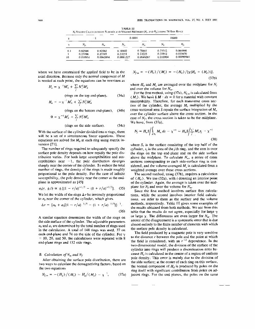
TABLE 111 Nf VALUES CALCULATED BY SURFACE AND VOLUME METHODS (NjA AND N,,,) USING 74 SIDE RINGS

X - 1 0.0001 10000

Y Nfl Nf$ Nfl Nf, Nf,.

0.73312 0.064998 0.23258 0.23225 0.22912 0.015670

0.1 0.82568 0.82582 0.78460 0.7846 1 1 0.23196 0.23195

10 0.018951 0.0042004 0.0081227 0.0049267 0.016904 0.00099941

where we have constrained the applied field to be in the axial direction. Because only the normal component of M is needed at each point, the equations can be rewritten as

H, = x - ' M i + c NYML J

(rings on the top end-plane), (34a)

H, = - x - ' M ; + N,"M$ J

(rings on the bottom end-plane), (34b) o = x - l ~ ~ + C N Y M J ,

J

(rings on the side surface). (34c)

With the surface of the cylinder divided into n rings, there will be a set of n simultaneous linear equations. These equations are solved for M,, at each ring using matrix in- version [7 11.

The number of rings required to adequately specify the surface pole density depends on how rapidly the pole distribution varies. For both large susceptibilities and susceptibilities near - 1, the pole distribution diverges sharply near the corner of the cylinder. To reduce the total number of rings, the density of the rings is made roughly proportional to the pole density. For the case of infinite susceptibility, the pole density near the corner at the end- plane is approximated as [45]

uo(r, * 1 ) * [ ( 1 - r / a ) - 1 / 3 - (1 + (35)

We let the width of the rings A r be inversely proportional to uo near the comer of the cylinder, which gives

A r = {ao + a l [ ( l - r / ~ ) - " ~ - (1 + r / ~ ) - ' / ~ ] } - ' .

(36) A similar equation determines the width of the rings on the side surface of the cylinder. The adjustable parameters a. and a I are determined by the total number of rings used in the calculation. A total of 148 rings was used, 37 on each end-plane and 74 on the side of the cylinder. For y = 10, 20, and 50, the calculations were repeated with 8 end-plane rings and 132 side rings.

B. Calculation of N , and Nj After obtaining the surface pole distribution, there are

two ways to calculate the demagnetizing factors, based on the two equations

(37a) Nf,m = - ( H d ) / < M , > = H , / ( M , ) - x - I ,

where Hd and M, are averaged over the midplane for Nf and over the volume for N,.

For the first method, using (37a), N f , , is calculated from ( M,). We have $ M ds = 0 for a material with constant susceptibility. Therefore, for each transverse cross section of the cylinder, the average M, multiplied by the cross-sectional area S equals the surface integration of M,, over the cylinder surface above the cross section. In the case of N f , the cross section is taken to be the midplane. We have, from (37a),

(38) where SI is the surface consisting of the top half of the cylinder, sj is the area of thejth ring, and the sum is over the rings on the top end-plane and on the side surface above the midplane. To calculate N,, a series of cross sections corresponding to each side-surface ring is considered, and the volume-averaged M, is calculated from a weighted average over these cross sections.

The second method, using (37b), requires a calculation of ( Hd ) . We use (32a), with i denoting an interior point of the cylinder. Again, the average is taken over the midplane for Nf and over the volume for N,.

Since the first method involves surface flux calculations, while the second involves interior field calculations, we refer to them as the surface and the volume methods, respectively. Table I11 gives some examples of the results obtained from both methods. We see from this table that the results do not agree, especially for large y or large x. The differences are even larger for N,. The source of the disagreement is a systematic error that is due almost entirely to the finite number of elements with which the surface pole density is calculated.

The field produced by a magnetic pole is very sensitive to the distance r between the pole and the point at which the field is considered, with an r P 2 dependence. In the two-dimensional model, the division of the surface of the cylinder into rings will produce a discretization error because Hd is calculated in the center of a region of Uniform pole density. This error is mainly due to the division of the side surface; at the center of each ring on this surface, the normal component of Hd is produced by poles on the ring itself with significant contribution from poles on adjacent rings. For the end planes, the poles on the same

I U I

CHEN et a l . : DEMAGNETIZING FACTORS FOR CYLINDERS 3609

0

-0.5

1 0 r / a

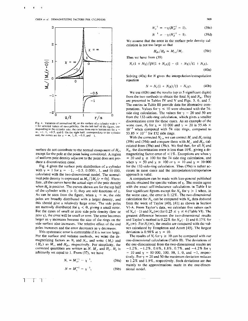
Fig. 4 . Variation of normalized M,, on the surface of a cylinder with y = 1 for selected values of susceptibility. On the left half of the figure, corresponding to the cylinder side, the curves from top to bottom are for x = 03, - 1 , 1, -0.5, and 0. On the right half, corresponding to the cylinder end, the curves are for x = 00, 1 , 0, -0.5, and - 1 .

surface do not contribute to the normal component of H d , except for the pole at the point being considered. A region of uniform pole density adjacent to the point does not produce a discretization error.

Fig. 4 gives the surface pole distribution of a cylinder with y = 1 for x = -1, -0.5, 0.0001, 1, and 10 000, calculated with the two-dimensional model. The normalized pole density is expressed as M , / I M,, ( r = 0) I . There- fore, all the curves have the actual sign of the pole density when H, is positive. The curves shown are for the top half of the cylinder with z > 0; they are odd functions of z . As can be seen from the figure, when x --$ 00, the side poles are broadly distributed with a larger density, and this should give a relatively large error. The side poles are narrowly distributed for x < 0, giving a small error. For the cases of small or zero side-pole density (low or zero x ) , the error will be small or zero. The error becomes larger as y increases because the size of the rings on the side surface also increases. The relative effect of the end poles increases and the error decreases as y decreases.

This systematic error is correctable if it is not too large. For the surface and volume methods, we write the demagnetizing factors as Ns and N,,, and write ( M , ) and ( H d ) as M,, and Hdr,, respectively. For simplicity, the corrected quantities are written as N , M,, and H d . Ha is arbitrarily set equal to 1. From (37), we have

(394 N = M - ' - - I zs x ,

N,' = - x ( H i ; + l),

N - ' = - x ( H d l + 1).

(39c)

(394

We assume that the error in the surface pole density calculation is not too large so that

H d u / H d M z s / M z . (39e)

Thus we have from (39)

NJl + N x ) / [ N ( l + Nvx)l = (1 + N x ) / ( 1 + N , X ) .

(404

Solving (40a) for N gives the interpolation/extrapolation equation

(40b)

We use (40b) and the results (up to 5 significant digits) from the two methods to obtain the final Nf and N,. They are presented in Tables IV and V and Figs. 5, 6 , and 7. The entries in Table I11 provide data for illustrative com- putations. Values for y I 10 were obtained with the 74- side-ring calculation. The values for y = 20 and 50 are from the 132-side-ring calculation, which gives a smaller discretization error for these cases. As an example of the worst case, Nf for x = 10 000 and y = 20 is 55.46 X

lop4 when computed with 74 side rings, compared to 53.85 x lop4 for 132 side rings.

With the corrected Nf, , we can correct M, and Hd using (39b) and (39d) and compare them with M z s and Hdt, calculated from (39a) and (39c). We find that, for all Nf and N,, the discretization error is less than l o % , giving a demagnetizing factor error of < l %. Exceptions are when y = 20 and x 2 100 for the 74-side-ring calculation, and when y = 50 and x 2 100 or y = 10 and x = 10 000 for the 132-side-ring calculation. Thus (39e) is rather accurate in most cases and the interpolation/extrapolation approach is valid.

A comparison can be made with less-general published results obtained for specific values of x . The results agree with the exact self-inductance calculations in Table I to four significant figures except for N , for y > 1 when, in the worst case, the error is 0.12%. The two-dimensional calculation for N , can be compared with N , data deduced from the work of Taylor [40], [41] as shown in Section VI-A. From Taylor's data, we calculate five values each of N m ( - 1) and N , ( m ) for 0.25 I y I 4 (Table VI). The greatest difference between the two-dimensional results and Taylor's method is 0.22% for N,( - 1 ) and 0.17% for N , (00). For Nf(03) , the results are compared with the values calculated by Templeton and Arrott [45]. The largest deviation is 0.98% at y = 10.

The results of Nf for y 1 10 can be compared with our one-dimensional calculation (Table 11). The deviations of the one-dimensional from the two-dimensional results are -1.2%, -1.2%, 0.6%, 1.8%, 0 .7%, and -4.2% f o r y = 10 and x = 10 000, 100, 10, 1, 0, and - 1, respectively. For y = 20 and 50 the maximum deviation reduces to 1.2% and 1.9%, respectively. Such deviations are due mainly to the approximations made in the one-dimensional model.

N = Nr)(1 + N s x ) / ( 1 + N,,x) .


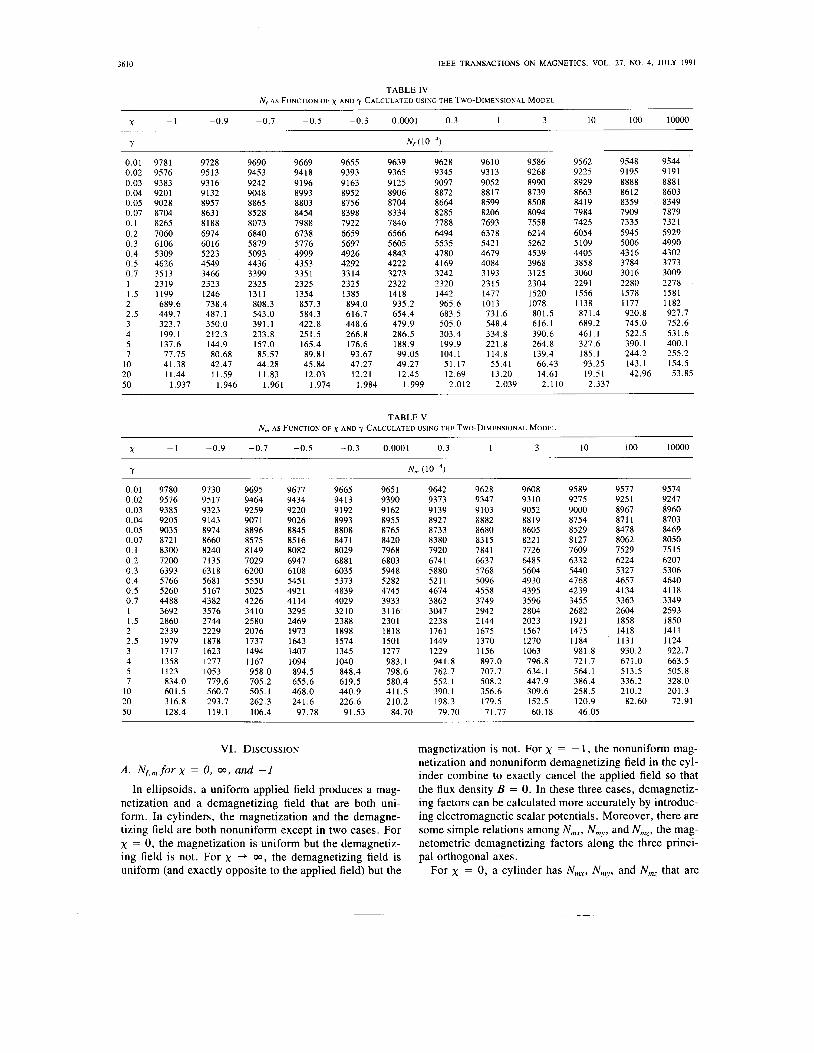
TABLE IV N, AS FUNCTION OF x A N D y CALCULATED USING THE TWO-DIMENSIONAL MODEL

X 10 100 10000 -1 -0.9 -0.7 -0.5 -0.3 0.0001 0.3 1 3

Y

0.01 0.02 0.03 0.04 0.05 0.07 0.1 0.2 0.3 0.4 0.5 0.7 1 1.5 2 2.5 3 4 5 7

10 20 50

N,

9781 9576 9383 9201 9028 8704 8265 7060 6106 5309 4626 3513 2319 1199 689.6 449.7 323.7 199.1 137.6 77.75 41.38 11.44

1.937

9728 9513 9316 9132 8957 863 1 8188 6974 6016 5223 4549 3466 2323 1246 738.4 487.1 350.0 212.3 144.9 80.68 42.47 11.59

1.946

9690 9453 9242 9048 8865 8528 8073 6840 5879 5093 4436 3399 2325 131 1 808.3 543.0 391.1 233.8 157.0 85.57 44.28 11.83

1.961

9669 9418 9196 8993 8803 8454 7988 6738 5776 4999 4353 335 1 2325 1354 857.3 584.3 422.8 251.5 165.4 89.81 45.84 12.03

1.974

9655 9393 9163 8952 8756 8398 7922 6659 5697 4926 4292 3314 2325 1385 894.0 616.7 448.6 266.8 176.6 93.67 47.27 12.21

1.984

9639 9628 9365 9345 9125 9097 8906 8872 8704 8664 8334 8285 7846 7788 6566 6494 5605 5535 4843 4780 4222 4169 3273 3242 2322 2320 1418 1442 935.2 965.6 654.4 683.5 479.9 505.0 286.5 303.4 188.9 199.9 99.05 104.1 49.27 51.17 12.45 12.69

1.999 2.012

9610 9313 9052 8817 8599 8206 7693 6378 542 1 4679 4084 3193 2315 1477 1013 731.6 548.4 334.8 221.8 114.8 55.41 13.20 2.039

9586 9268 8990 8739 8508 8094 7558 6214 5262 4539 3968 3125 2304 1520 1078 801.5 616.1 390.6 264.8 139.4 66.43 14.61 2.110

9562 9225 8929 8663 8419 7984 7425 6054 5 109 4405 3858 3060 2291 1556 1138 871.4 689.2 461.1 327.6 185.1 93.25 19.51 2.337

9548 9544 9195 9191 8888 8881 8612 8603 8359 8349 7909 7879 7335 7321 5945 5929 5006 4990 4316 4302 3784 3773 3016 3009 2280 2278 1578 1581 1177 1182 920.8 927.7 745.0 752.6 522.5 531.6 390.1 400.1 244.2 255.2 143.1 154.5 42.96 53.85

TABLE V N , AS FUNCTION OF x AND CALCULATED USING THE TWO-DIMENSIONAL MODEL

X 3 10 100 10000 -1 -0.9 -0.7 -0.5 -0.3 0.0001 0.3 1

0.01 0.02 0.03 0.04 0.05 0.07 0.1 0.2 0.3 0.4 0.5 0.7 1 1.5 2 2.5 3 4 5 7

10 20 50

9780 9576 9385 9205 9035 872 1 8300 7200 6393 5766 5260 4488 3692 2860 2339 1979 1717 1358 1123 834.0 601.5 316.8 128.4

9730 9517 9323 9 143 8974 8660 8240 7135 6318 5681 5167 4382 3576 2744 2229 1878 1623 1277 1053 779.6 560.7 293.7 119.1

9695 9464 9259 907 1 8896 8575 8149 7029 6200 5550 5025 4226 3410 2580 2076 1737 1494 1167 958.0 705.2 505.1 262.3 106.4

9677 9434 9220 9026 8845 8516 8082 6947 6108 545 1 492 1 41 14 3295 2469 1973 1643 1407 1094 894.5 655.6 468.0 241.6

97.78

9665 9413 9 192 8993 8808 847 1 8029 6881 6035 5373 4839 4029 3210 2388 1898 1574 1345 1040 848.4 619.5 440.9 226.6

91.53

965 1 9390 9162 8955 8765 8420 7968 6803 5948 5282 4745 3933 3116 2301 1818 1501 1277 983.1 798.6 580.4 411.5 210.2

84.70

9642 9373 9139 8927 8733 8380 7920 6741 5880 521 1 4674 3862 3047 2238 1761 1449 1229 941.8 762.7 552.1 390.1 198.3 79.70

9628 9347 9103 8882 8680 8315 7841 6637 5768 5096 4558 3749 2942 2 144 1675 1370 1156 897.0 707.7 508.2 356.6 179.5 71.77

9608 93 10 9052 8819 8605 822 1 7726 6485 5604 4930 4395 3596 2804 2023 1567 1270 1063 796.8 634.1 447.9 309.6 152.5 60.18

9589 9275 9000 8754 8529 8127 7609 6332 5440 4768 4239 3455 2682 1921 1475 1184 981.8 721.7 564.1 386.4 258.5 120.9 46.05

9577 925 1 8967 8711 8478 8062 7529 6224 5327 4657 4134 3363 2604 1858 1418 1131 930.2 671.0 513.5 336.2 210.2

82.60

9574 9247 8960 8703 8469 8050 7515 6207 5306 4640 4118 3349 2593 1850 141 1 1124 922.7 663.5 505.8 328.0 201.3 72.91

VI. DISCUSSION

A . Nf,, f o r x = 0, 00, and -1

In ellipsoids, a uniform applied field produces a magnetization and a demagnetizing field that are both uniform. In cylinders, the magnetization and the demagnetizing field are both nonuniform except in two cases. For x = 0, the magnetization is uniform but the demagnetizing field is not. For x + 03, the demagnetizing field is uniform (and exactly opposite to the applied field) but the

magnetization is not. For x = - 1, the nonuniform magnetization and nonuniform demagnetizing field in the cylinder combine to exactly cancel the applied field so that the flux density B = 0. In these three cases, demagnetizing factors can be calculated more accurately by introduc- ing electromagnetic scalar potentials. Moreover, there are some simple relations among N,, Nmy, and NmZ, the magnetometric demagnetizing factors along the three principal orthogonal axes.

For x = 0, a cylinder has N,,, Nmy, and N,, that are

I II I

CHEN er al.: DEMAGNETIZING FACTORS FOR CYLINDERS

c z

1 .o

0.8

0.6

0.4

0.2

0.0 0.01 0.1 1 10

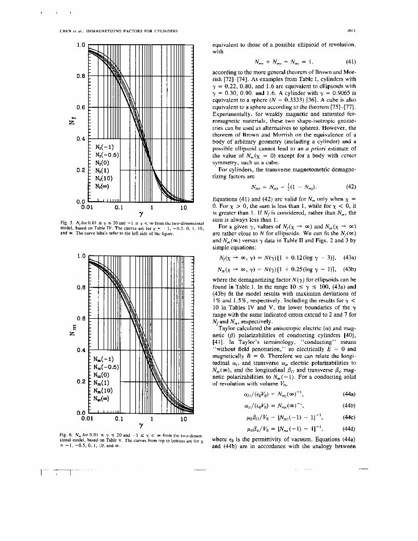
Y Fig. 5 . Nffor 0.01 5 y 5 20 and - 1 5 x < 01 from the two-dimensional model, based on Table IV. The curves are for x = - 1 , -0.5, 0, 1 , 10, and OD. The curve labels refer to the left side of the figure.

1 .o

0.8

0.6

E z

0.4

0.0 o.2i 0.01 0.1

Y 1 10

Fig. 6. N, for 0.01 I y 5 20 and - 1 5 x < 01 from the two-dimensional model, based on Table V . The curves from top to bottom are for x = - 1 , -0.5, 0, 1, 10, and 00.

3611

equivalent to those of a possible ellipsoid of revolution, with

N , + Nmy + N,, = 1, (41)

according to the more general theorem of Brown and Mor- rish [72]-[74]. As examples from Table I, cylinders with y = 0.22, 0.80, and 1.6 are equivalent to ellipsoids with y = 0.30, 0.90, and 1.6. A cylinder with y = 0.9065 is equivalent to a sphere ( N = 0.3333) [36]. A cube is also equivalent to a sphere according to the theorem [75]-[77]. Experimentally, for weakly magnetic and saturated ferromagnetic materials, these two shape-isotropic geometries can be used as alternatives to spheres. However, the theorem of Brown and Monish on the equivalence of a body of arbitrary geometry (including a cylinder) and a possible ellipsoid cannot lead to an a priori estimate of the value of N , ( x = 0) except for a body with center symmetry, such as a cube.

For cylinders, the transverse magnetometric demagnetizing factors are

(42)

Equations (41) and (42) are valid for N , only when x = 0. For x > 0, the sum is less than 1, while for x < 0, it is greater than 1. If Nf is considered, rather than N,,,, the sum is always less than 1.

For a given y, values of N f ( x -+ 00) and N,(x -, 03) are rather close to N for ellipsoids. We can fit the Nf(03) and N , (03) versus y data in Table I1 and Figs. 2 and 3 by simple equations:

N , = Nmy = i (1 - NmJ.

N ~ ( x -+ 03, y) = N ( y ) [ l + 0.12(log - 3)1, (43a)

Nm ( X + 00, 7) = N ( y ) [1 + 0.25 (log - I)], (43b)

where the demagnetizing factor N ( y ) for ellipsoids can be found in Table I. In the range 10 I y I 100, (43a) and (43b) fit the model results with maximum deviations of 1 % and 1.5 % , respectively. Including the results for y < 10 in Tables IV and V, the lower boundaries of the y range with the same indicated errors extend to 2 and 7 for Nf and N,, respectively.

Taylor calculated the anisotropic electric (CY) and magnetic (0) polarizabilities of conducting cylinders [40], [4 13. In Taylor’s terminology, “conducting” means “without field penetration,” so electrically E = 0 and magnetically B = 0. Therefore we can relate the longitudinal CY/ and transverse CY,, electric polarizabilities to Nm(03) , and the longitudinal and transverse P,, magnetic polarizabilities to N , (- 1). For a conducting solid of revolution with volume Vo,

CY/ , / (EOVO/O) = Nrnz(W)-’, e a )

C Y f f / ( % ~ O ) = Nm(03>-’ , ( a b )

P O P / / / V O = [Nrnz(-l) - 11-’9

cC,P,lV, = W A - 1 ) - 11-13

(UC)

( a d )

where eo is the permittivity of vacuum. Equations (44a) and (44b) are in accordance with the analogy between

3612

1

0.1 z

z SE

0.01

0.01 0.1 1 10 Y (a)

IEEE TRANSACTIONS ON MAGNETICS, VOL. 27, NO. 4, JULY 1991

0.25

0.20

0.15 z“

0.10

0.05

0.00 1 2 3 4 5 6 7 8 9 10

Y (b)

Fig. 7 . N , (solid curves) and N,(dashed curves) from the two-dimensional model. (a) Logarithmic scale, 0.01 I y I 20. The curve labels refer to the right side of the figure. (b) Linear scale, 1 I y I 10.

TABLE VI N,,(m), N,.x(m), Nmz(-1), and Nmx(-I) FORSHORTCYLINDERS~

y N,,(m) N,,(m)

0 1 0 0.25 0.5712 0.1618 0.5 0.4111 0.2371 1 0.2590 0.3154 2 0.1409 0.3829 4 0.06635 0.4319 m 0 0.5

E(m) N,??:(-I)

1 1 0.8948 0.6764 0.8853 0.5258 0.8895 0.3692 0.9067 0.2341 0.9302 0.1361 1 0

N,, ( - 1 )

0 0.2136 0.2928 0.3669 0.4237 0.4596 0.5

E ( - l )

1 1.1036 1.1114 1.1030 1.0815 1.0553 1

“The data are obtained from the electric and magnetic polarizabilities of conducting cylinders calculated by Taylor 1401, 1411. E (m) and E ( - 1) are t h e s u m s N , , + N , , + N , : f o r x ~ m a n d X = - 1 .

electrostatic shielding in a conductor and magnetostatic shielding in the same body but with x -+ 03.

There is a relation between and at, [41],

POPI[ = - C Y Y , m O ) , (454 which leads to an exact relation between N,,(m) and

N,(@) = Nmy(@) = ;[I - Nmz(-l)]. (45b)

TableVIlists Nmz(oo),Nm(@), N,,(-l), andNm(-1) for short cylinders based on the CY and p data given by Taylor. From this table we see that the sum of the N,’s deviate from 1 by about 1 1 %. For other values of x , the deviation should be less, and this could help one estimate N,, for different values of x and y.

Nm, ( - 1) 9

B. General Rules for Nf and N, as Functions of x and y

We give some general rules for the variation of Nf and N , with y and x based on the tables and figures. (a) For a given x , both Nf and N , decrease with increasing y. This is because the demagnetizing effect is an “end effect,” although the demagnetizing fields depend on both end and side surface poles. When y increases, the effect of cylinder ends on the midplane and the entire volume decreases. (b) When both y and x are fixed, N,,,(y, x) > Nf(y, x). That is, the end effect is weaker at the midplane. (c) N,,, decreases with increasing x at any y. (d) With increasing x , Nf increases when y > 1 and decreases when y < 1; there is a region around y = 1 where Nf is insensitive to x. Rules (b), (c), and (d) give the following relation for Nf(x) and N , (x) when y > 1 :

Nrn(-l) > Nrn(0) > Nm(03) > Nf(@)

> Nf(0) > Nf(-l). (46) (e) For y > 1 , the ratio N,,,/Nfincreases with increas-

ing y and decreasing x . When y increases from 1 to 10 to 1000, N,(O)/N’(O) increases from 1.37 to 8 to 800; N, (03) / N f ( m ) is smaller and increases from 1.14 to 1.32 to 1.46. (f) The minimum x for Nf(x) > O.99Nf(m) increases with increasing y. In fluxmetric ferromagnetic measurements, this rule tells us that can be used for dM/dH larger than a minimum value that depends on y. For y = 10, 100, and 1000, the minimum values are 200, 5 X lo4, and lo6.

I II I

CHEN er al. : DEMAGNETIZING FACTORS FOR CYLINDERS

4 0 I

3.0 n 0 U

(a) 5 2 . 0 N W s!

1.0

0.0

1

-0.5 -1 3.0 1

0.001

CI Y

U +

1.0 (c) <

n

b W

0.0

- 1 . 0 0 1 .o :fi 0.0

1.0002

1.oooo . x =0.001 n e

v f l

SI

h0.9eoE - N v

0.98BE -

0.0002 -

a o.0000 X x =0.001 h J-o.oooz - z

-0.0004 -

0.0006 -

-0.0002 I 1

1 .o z"i: 0.0

Fig. 8 . M(z) /M(O) [graphs (a) and (d)]. H d ( z ) / H a [graphs (b) and (e)], and o ( z ) / o ( + l ) [graphs (c) and (f)] as functions of z / l for a cylinder with y = 20. The curves in graphs (a), (b), and (c) are for x = - 1 , -0.5, 0.001, 30, and lo5, respectively. Graphs (d), (e), and ( f ) are for x = 0.001 on an expanded scale.

C. Minimum x for N f ( x ) > 0 . 9 9 N f ( m )

For x > 0, the demagnetizing effect resembles the re- sponse of an amplifier with negative feedback. The input, output, and gain of the amplifier are Ha, M, and x , respectively. After operation, M becomes Hd(Hd = - N M , where N is the local demagnetizing factor), with sign opposite to that of Ha, which feeds back to the input. The result is that M becomes smaller and nonuniform, while H becomes smaller than Ha. There is perfect feedback when x -+ 03, and H = 0 everywhere. Since H / H a = (1 + N x ) - ' , where N is the local demagnetizing factor, in order to have N f ( x ) almost equal to N f ( m ) , (1 + N x ) must be sufficiently large for H I H , to be small everywhere. Actually Nf is the smallest local N , and the origin of rule (f) may be understood as follows.

N f ( w ) decreases with increasing y. To have N f ( x ) almost equal to Nf(03) , a smaller N f ( w ) must be balanced by a larger x to fulfill the condition of a sufficiently large (1 + N x ) . Therefore, with increasing y, the minimum x to satisfy N f ( x ) > 0 . 9 9 N f ( w ) increases. From Table I1 we can deduce this minimum x to be k / N f ( w ) with 15 < k < 17.

D. Position Dependence of M , H d , and 0

We have explained rules (a), (b), and (f). To understand the other rules, we have to know the details of the position dependence of M , H d , and a. Fig. 8(a), 8(b), and 8(c) gives the curves of M ( z ) / M ( O ) , Hd(Z)/Ha, and a(z)/a(+Z) as functions of z for y = 20 and x = -1, -0.5, 0.001, 30, and lo5 computed from the one-dimensional model with n = 10. Bloomberg and Arrott [78] derived M ( z ) / M ( O ) , using a similar approach, for 1 I x < w and y = 100. Our curves for x = 0.001 are replot- ted in Fig. 8(d), 8(e), and 8(f) on finer scales. When Ha is positive, M ( 0 ) and a( + 1 ) are positive for x > 0 and negative for x < 0. Therefore, for x = -0.5 and -1, the signs for M ( z ) and ~ ( z ) are opposite to the signs shown for M ( i ) / M ( O ) and a ( z ) / a ( + Z ) in Fig. 8(a) and 8(c). Also, M ( z ) and & ( z ) are even functions of z , but a ( z ) iS

an odd function of z .

E. x Dependence of N,,,/Nf For x = lo5 (that is, x -+ w) we can see in Fig. 8(b)

that Hd(z ) is a constant equal to -Ha in the entire cylinder, which makes H very small (0 for x -, 00) and M ( z )

-1- 7--lr--- - --


finite. M ( z ) is approximately parabolic as shown in Fig. 8(a) and as already pointed out by other authors [2 11, [27]. The average Hd is equal to - H a . For the midplane and the entire volume, respectively, the average M is M ( 0 ) and approximately 0.67M(O). Therefore, N,, , /Nf should be close to 1.5.

When x decreases to 30, the variation of M ( z ) is grad- ual for small ? and sudden in the end regions. This increases the volume-averaged M to more than 0.67M(O). But because Hd ( z ) becomes rather z dependent and its absolute value at z = 1 is much larger than at z = 0 [Fig. 8(b)], N , / N f is larger.

As x decreases to 0.001, both M ( z ) and Hd(z ) remain nearly constant in Fig. 8(a) and 8(b). The reason is that M ( z ) is very small compared to Ha, so &(I) is even smaller than H,. The variation of the extremely small Hd(z ) cannot be seen in Fig. 8(b), and the modification of the field by such a small Hd ( z ) causes an invisible change in M in Fig. 8(a). However, if we expand the scales [Fig. 8(d) and 8(e)], we can see that the variation of M ( z ) and Hd(z ) continues the trend of decreasing x from lo5 to 30. This makes N , / N f even larger.

When x is small but negative, both M ( z ) and Hd(z ) change their signs. At this point, Nf and N,,, continue the trend without sudden change. The situation for x < 0 can be seen from the curves for x = -0.5 and - 1 in Fig. 8(a) and 8(b). For these two cases, Hd(z ) and the absolute value of M ( z ) remain constant until z > 0.81, and then they suddenly increase. This makes N , / N f largest when x = - 1 . Further discussion of this in terms of pole distribution is given in the next section.

F. x Dependence of Nf

To understand the susceptibility dependence of Nf for y > 1, we focus on the magnetic pole distribution shown in Fig. 8(c) and 8(f). For the largest x , a(z) varies with z almost linearly on the cylinder surface except for the regions close to the ends. This means that the magnetic poles are the most uniformly distributed on the cylinder, and Hd (0), which has a greater contribution from the poles in the central region than from the ends, is the largest. Thus Nf is its largest for the highest x .

When x is decreasing, the variation of u(z) is progres- sively greater in the end regions, while the magnetic pole density in the central region becomes gradually lower. Therefore, Nf decreases with decreasing x . When x = 0, all the poles are at the ends, a(z) is 0, and Nf should be its smallest. In fact, Nf continues to decrease when x becomes negative. The reason is that, although a(x) remains 0 in a large central region for x < 0, a(z) for z close to 1 increases with decreasing x and its sign is opposite to that of a( + 1 ) [Fig. 8(c)]. The side poles produce a field at the center directed opposite to the field produced by the end poles, so that the demagnetizing effect of the end poles is partially compensated by the effect of the side poles. This makes Nf a little lower than for x = 0. The side poles close to the ends, with signs opposite to those of the end poles, have a different effect on N,. They greatly increase the value of Hd in the end regions, so the volume-aver-

aged N,,, increases with decreasing x even for negative x. Finally, we have the largest value of N , / N f at x = - 1 .

When y < 1, the susceptibility dependence of Nf is the opposite. We can explain this as follows. For oblate cylinders, the end poles are the main contributors to the demagnetizing field Hd at the midplane. For a given ( M , ) at the midplane, the end-pole density is smallest when x -+ 00 since, in this case, the poles are the most uniformly distributed on the entire surface. Therefore Nf is the smallest. A smaller positive x repels the poles to the end regions, which gives rise to a larger end-pole density and a larger N f . Although all the poles are distributed on the ends when x = 0, the pole density on the ends is not the largest. This is because, when x < 0, the end-pole density has a sign opposite to that of the side-pole density nearby, as can be seen from Fig. 4; thus the end poles are further enhanced. As a consequence, the end pole density increases continuously with decreasing x regardless of its sign, and Nf takes its largest value when x = - 1 .

G. Error Transmission in Susceptibility Measurements From the above analysis we see that, at present, the

accuracy of N , and Nf can reach 1 % in general. To know if this accuracy is good enough for the purpose of magnetic measurements, we examine the influence of the error in N,,, or Nf on susceptibility measurements. We consider a cylinder consisting of material with constant x in a longitudinal applied field Ha. An external susceptibility xe can be defined as ( M ) / H a , where the average is taken over the whole volume or the midplane, depending on whether N , or Nf is considered. From (3), replacing N by Nf,,,, and M by ( M ), we obtain

x = x e ( 1 - Nf,mxc)-l* (47)

This equation is accurate under the above assumptions and definitions. From (47), the relative error in x caused by the calculation error of Nf, ,,, and the measurement error of x e can be derived as

I A X / X I = INf.rnxl lANf,rn/N~ml + ( x / x A IAxelxel .

(48)

On the right-hand side of (48), the first term is the transmission error from the erroneous Nf, , calculation to the x determination. This error equals the error in Nf,, multiplied by a factor a1 = I N f , , x ( , which can be obtained from the results of this work. We examine three typical cases. In the first case, I x ( and a l are small; the error in Nf,,,, can be large and still result in a small trqns- mission error. For example, when I x( = 0.1, we have al < 0.1 since Nf,,,, < 1 , and less than 10% of the N f , , error is reflected in the final x result. The second case is a magnetometric measurement for x = - 1 . c y 1 , obtained from Table V, is 0.37, 0.17, and 0.06 for y = 1, 3, and 10; only a small part of the error in N,,, is transmitted to the final x result. In the third case, high-x materials are considered. To reduce the error due to the large a l , fluxmetric measurements should be made with long samples, since Nf < N,,, and Nf decreases with increasing y. To

I II I

CHEN er al . : DEMAGNETIZING FACTORS FOR CYLINDERS 3615

ensure that aI < 1 based on Table I1 and Fig. 2, y should be 12, 58, 200, and 700, for x = lo2, lo3, lo4, and lo5, respectively.

The second term in (48) is the transmission error due to the measurement error of xe. The corresponding factor is a2 x/xe. For the first case where cyI is very small, a2 is very close to 1 since x = xe, so the error in x is almost the same as the xe measurement error. For our second case, from (47), we have al + a2 = 1 . This is inter- esting because, when y is small so that N, + 1 and a1 +

1, the x error is mainly due to the error in N,, no matter how large the xe measurement error is. For the high-x case, if a1 = 1 , we have a2 = 2 from (47), leading to a double transmission error to x from the xe measuring error. As a consequence, to obtain accurate results of x for high-x materials, both accurate Nf and accurate xe are strongly required if y cannot be made very large.

In summary, to determine x accurately, the higher the I X I of the material, the higher is the required calculation accuracy of Nf,,. From a magnetic measurement point of view, our calculation accuracy for Nf., at x = 0 is more than adequate, and the number of calculated points is suf- ficient for accurate interpolation over a wide range of values. For other x values, the requirement for calculation accuracy will be determined by the particular purpose of the magnetic measurement; a 1% accuracy may be suffi- cient for many uses but is inadequate for others. For example, our 0.2% accuracy for x = -1 is required for superconductor calibration standards.

H . Application to Materials with x > 0 Most materials have x > 0, and our results can be used

for demagnetization corrections of their magnetic measurements. For materials with linear or nearly linear magnetization curves, our Nf,, values are satisfactory. These include paramagnets, spin glasses, weakly magnetic materials, and iron-powder cores and ordinary ferromagnets in the initial and saturation states. However, even in these cases, some caution is required. We give an example below.

For magnetometric measurements of weakly magnetic materials (x < 0.01) only very small demagnetizing corrections are needed. However, such materials can also be measured by fluxmetric methods, as recommended by at least one measurement standard [79]. A source of error in fluxmetric measurements is if the sample diameter is less than that of the measurement coil. A large demagnetizing effect would occur in the measurement of M because the measured flux linkage is contributed not only by the M of the sample but also by the Hd within the coil volume produced by the sample’s poles. Furthermore, fluxmetric measurements on weakly magnetic materials require many coil turns, which ensures that this error will arise. The error in x due to this effect can be as large as 30%, even if the requirements of [79] are followed [38], [64].

The magnetization curves of ferromagnetic materials are nonlinear, and it is difficult to assign to them specific x and Nf,,(x) values except in the initial state and when approaching saturation, as mentioned above. However,

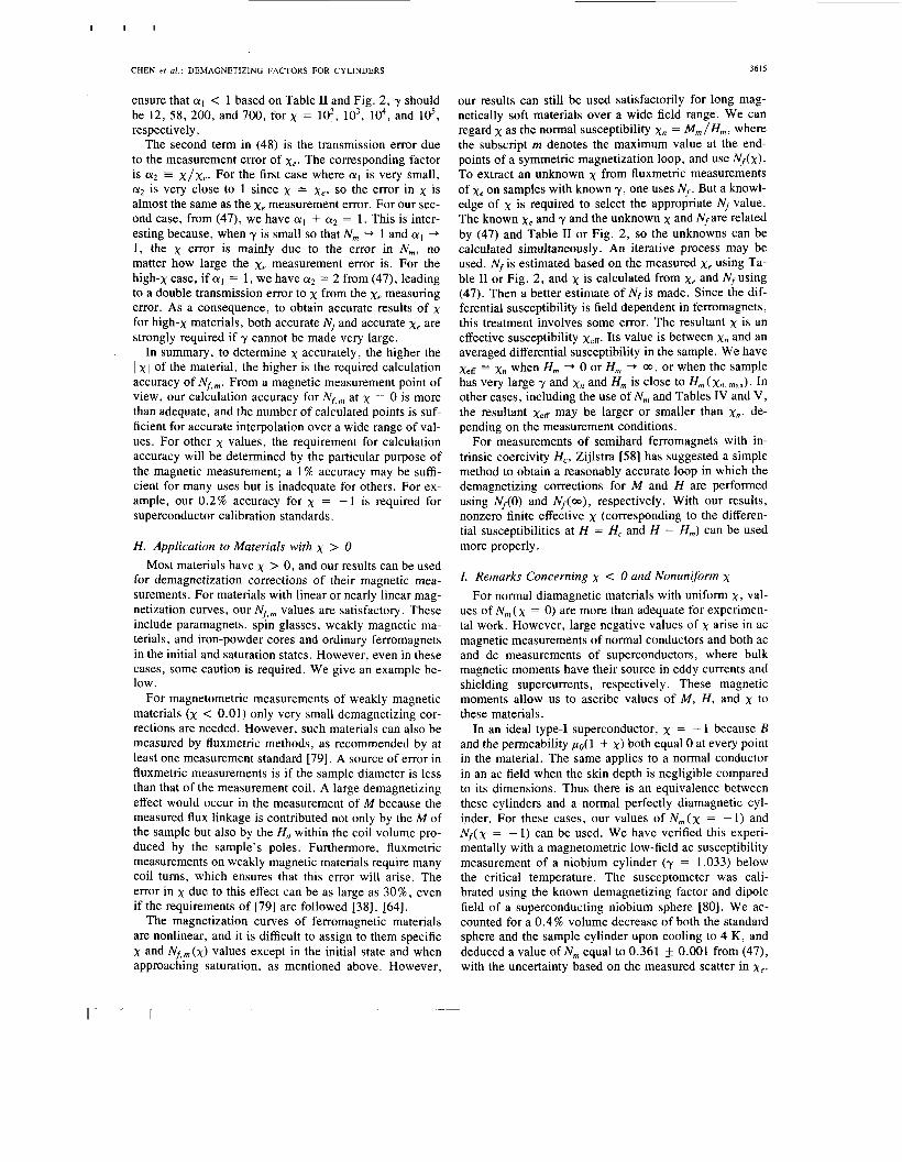
our results can still be used satisfactorily for long magnetically soft materials over a wide field range. We can regard x as the normal susceptibility x,, = M , / H , , where the subscript m denotes the maximum value at the end- points of a symmetric magnetization loop, and use Nf(x). To extract an unknown x from fluxmetric measurements of xe on samples with known y, one uses Nf. But a knowl- edge of x is required to select the appropriate Nf value. The known xe and y and the unknown x and Nfare related by (47) and Table I1 or Fig. 2, so the unknowns can be calculated simultaneously. An iterative process may be used. Nf is estimated based on the measured xe using Ta- ble I1 or Fig. 2, and x is calculated from xe and Nfusing (47). Then a better estimate of Nf is made. Since the differential susceptibility is field dependent in ferromagnets, this treatment involves some error. The resultant x is an effective susceptibility xeff. Its value is between x,, and an averaged differential susceptibility in the sample. We have xeff = x,, when H , --$ 0 or H , + 03, or when the sample has very large y and x,, and H , is close to H , ( x,,, ,,,). In other cases, including the use of N, and Tables IV and V, the resultant xeff may be larger or smaller than xn, depending on the measurement conditions.

For measurements of semihard ferromagnets with in- trinsic coercivity H,, Zijlstra [58] has suggested a simple method to obtain a reasonably accurate loop in which the demagnetizing corrections for M and H are performed using Nf(0) and Nf(03), respectively. With our results, nonzero finite effective x (corresponding to the differential susceptibilities at H = H , and H = H,) can be used more properly.

I . Remarks Concerning x < 0 and Nonuniform x For normal diamagnetic materials with uniform x, val-

ues of N, ( x = 0) are more than adequate for experimental work. However, large negative values of x arise in ac magnetic measurements of normal conductors and both ac and dc measurements of superconductors, where bulk magnetic moments have their source in eddy currents and shielding supercurrents, respectively. These magnetic moments allow us to ascribe values of M , H , and x to these materials.

In an ideal type-I superconductor, x = -1 because B and the permeability po( 1 + x) both equal 0 at every point in the material. The same applies to a normal conductor in an ac field when the skin depth is negligible compared to its dimensions. Thus there is an equivalence between these cylinders and a normal perfectly diamagnetic cylinder. For these cases, our values of N,,, ( x = - 1) and Nf( x = - 1) can be used. We have verified this experimentally with a magnetometric low-field ac susceptibility measurement of a niobium cylinder (y = 1.033) below the critical temperature. The susceptometer was cali- brated using the known demagnetizing factor and dipole field of a superconducting niobium sphere [80]. We ac- counted for a 0.4% volume decrease of both the standard sphere and the sample cylinder upon cooling to 4 K, and deduced a value of N, equal to 0.361 0.001 from (47), with the uncertainty based on the measured scatter in xe.


Our two-dimensional calculations give 0.3622. Thus we see that cylindrical superconducting standards for magnetic measurements for use at low fields and temperatures can be made using accurate values of N , (- 1).

The results of this work have to be used more carefully for materials that do not have constant susceptibility. In these cases, an effective susceptibility should be found. For example, the M ( H ) curve of an ideal type-I1 superconductor in fields below the lower critical field H,, is linear, with x = - 1. In the mixed state, M ( H ) increases when H > H,, and the effective x should be close to the differential susceptibility at each point, which is positive. This causes a discontinuity in the value of N , above H,, , and a proper demagnetizing correction should take account of this effect. Similar caveats apply to the inter- mediate state of superconductors.

Normal conducting cylinders in ac fields have M ( H ) loops, and a complex susceptibility with a negative real part can be defined [81]. However, this susceptibility is due to eddy currents constrained by the skin effect, different from our model assumption of uniform susceptibility. Nf,, for x = - 1 may be used in the limit of small skin depth. Otherwise, to obtain good results, y must be large enough so that only a small correction is needed; our Nf,, values for an effective x < 0 can be used. A similar case arises in hard superconductors, where a por- tion of the magnetization comes from penetrated supercurrents that follow the critical-state model [82].

Since most cases of magnetic measurements involve nonlinear magnetization curves, the demagnetizing correction using the factors calculated for constant x should be made cautiously. For this, a deep understanding of the magnetization process and the ,demagnetizing effect is most important.

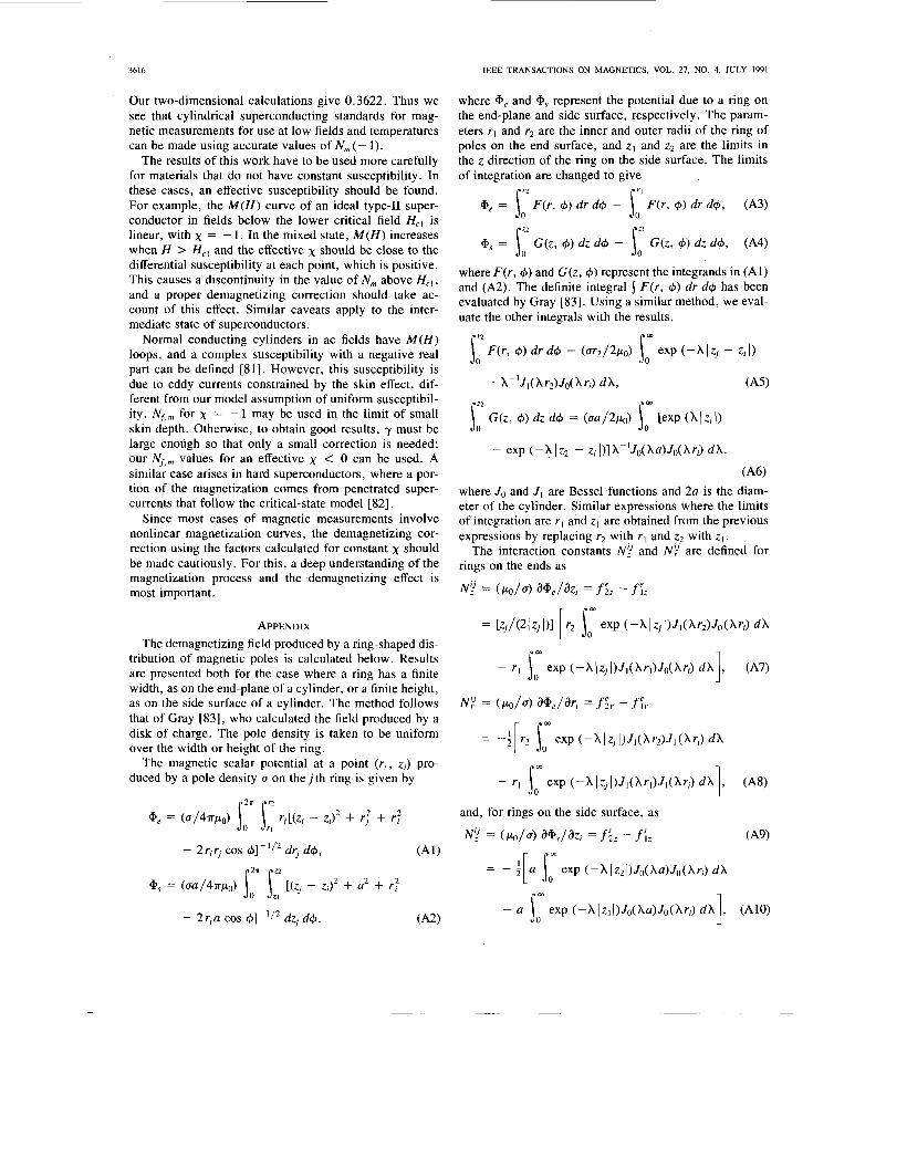
APPENDIX The demagnetizing field produced by a ring-shaped dis-

tribution of magnetic poles is calculated below. Results are presented both for the case where a ring has a finite width, as on the end-plane of a cylinder, or a finite height, as on the side surface of a cylinder. The method follows that of Gray [83], who calculated the field produced by a disk of charge. The pole density is taken to be uniform over the width or height of the ring.

The magnetic scalar potential at a point (rir z,) produced by a pole density U on the j t h ring is given by

9, = (U/4Tpo) 1; I n rj[(Zj - Zj)2 + rj + r:

- 2rjrj cos 4]-'12 drj d4, (All

+$ = (ua/4?rp0) S:" Sz* [(zj - zi)2 + a2 + r:

- 2 ~ i a COS dz, d4, ( A 3

where (P, and as represent the potential due to a ring on the end-plane and side surface, respectively. The parameters rl and r2 are the inner and outer radii of the ring of poles on the end surface, and zI and z2 are the limits in the z direction of the ring on the side surface. The limits of integration are changed to give

+e = p F(r , 4) dr d4 - j:' F(r, 4) dr d4 , (-43)

+s = sp G(z, 4) dz d4 - G(z, 4) dz d4 , (A4)

where F(r , 4) and G(z, 4) represent the integrands in (Al) and (A2). The definite integral S F ( r , 4) dr d4 has been evaluated by Gray [83]. Using a similar method, we eval- uate the other integrals with the results,

F(r, 4) dr d4 = (ur2 /2~0) som exp (-A I zj - zi I)

h-'J1(hr2)Jo(hri) d h , ('45)

(A61 where Jo and J I are Bessel functions and 2a is the diameter of the cylinder. Similar expressions where the limits of integration are r l and z1 are obtained from the previous expressions by replacing r2 with rl and z2 with z I .

The interaction constants NY and N:' are defined for rings on the ends as

N : = (Lco/u) a@.,/% = fS, - f4,

= rz,/<2lz,l>l[ r2 Iom exp (-xlz,I)Jl(hr2)JO(X~,) d h

- rl I exp ~ - ~ l z , l ~ J l ~ ~ ~ l ~ J o ~ ~ ~ , ~ d h ] , ('47)

= - ; [ r2 som exp (-A lz, I)JlW2)Jl O r , ) dX

- rl iom exp ( - ~ l z , l ) J l ( ~ ~ l ) J l ( ~ ~ l ~ d h ] , (A81

N : = (Po /4 a+.,/ar, = f S r - f ; r

and, for rings on the side surface, as

N:' = (PO/U> a+,/az, = fiz - f;, ('49)

= - ; [ a iom exp ( - h ~ ~ ~ ( ) J ~ ( X a ) J ~ ( h r , ) d h

1 - a 1, exp ~ - ~ I ~ ~ o ~ ~ ~ ~ ~ ~ ~ ~ ~ ~ ~ , > d h , (A101

I


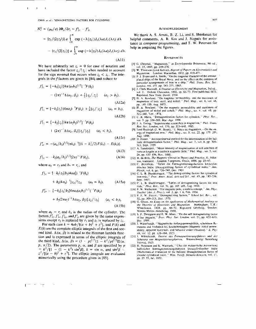
N : = ( p o / u ) a+.,/&-; = f i r - f i r

= [z2/(21z201 a iom exp (-hlz2l)J,(Xa)J,(Xr;) dX

- [z1/(21z101 a ’jomexp (-Xlzl()J,(Xa)Jl(Xr;) dX.

(AI 1)

We have arbitrarily set zi = 0 for ease of notation and have included the factor z,/ 1 zj I when needed to account for the sign reversal that occurs when zj < zi. The integrals in theffactors are given in [84] and reduce to

where a2 = r2 and b2 = ri, and

+ b2(2na2)Y1Mcy2, P2))z2/lz2l (a2 < b2),

(A15b)

where a2 = ri and b2 is the radius of the cylinder. The factors f;?, f&, f&, and f i r are given by the same expressions except r2 is replaced by rl and z2 is replaced by z I .

For each case k = 4ab/[(a + b)2 + z2], and F ( k ) and E ( k ) are the complete elliptic integrals of the first and second kind. A ( a , 6) is related to the Heuman lambda function and is expressed in terms of the elliptic integrals of the third kind, A(cy, P ) = (1 - p)’I2(1 - k 2 / p ) ’ k I ( a , p , 7r/2). The parameters p , cy, and 6 are specified by p = k 2 / [ 1 - (1 - k 2 ) sin2P], k = sin a, and sin2P = z2/[(a - b)2 + z 2 ] . The elliptic integrals are evaluated numerically using the procedure given in [MI.

ACKNOWLEDGMENT

We thank A. S. Arrott, B.-Z. Li, and S. Shtrikman for helpful comments, A. B. Kos and J. NoguCs for assis- tance in computer programming, and T. W. Petersen for help in preparing the figures.

REFERENCES

[I] G. Chrystal, “Magnetism,” in Encyclopaedia Brirannica, 9th ed.,

[2] W. Thomson (Lord Kelvin), Reprinf of Papers on Elecfrosfafics and Magnerism. London: Macmillan, 1872, pp. 470-471.

[3] F. J . Evans and A. Smith, “On the magnetic character of the armour- plated ships of the Royal Navy, and on the effect on the compass of particular arrangements of iron in a ship,” Phil. Trans. Roy. Soc. London, vol. 155, pp. 263-323, 1865.

[4] J . Clerk Maxwell, A Treafise on Elecfricify and Magnefism, 3rd ed., vol. 2. Oxford: Clarendon, 1892, pp. 66-73. First published 1873. Reprinted New York: Dover, 1954.

[5] H. A. Rowland, “On magnetic permeability, and the maximum of magnetism of iron, steel, and nickel,” Phil. Mag . , ser. 4, vol. 46,

[6] H. A. Rowland, “On the magnetic permeability and maximum of magnetism of nickel and cobalt,’’ Phil. Mag. , ser. 4, vol. 48, pp.

[7] C. R. Mann, “Demagnetization factors for cylinders,” Phys. Rev. , vol. 3, pp. 359-369, Mar.-Apr. 1896.

[8] J . A. Ewing, “Experimental researches in magnetism,” Phil. Trans. Roy. Soc. London, vol. 176, pp. 523-640, 1885.

[9] Lord Rayleigh (J. W. Strutt), “1. Notes on magnetism.-On the energy of magnetized iron,” Phil. Mag . , ser. 5 , vol. 22, pp. 175-183, Aug. 1886.

[IO] D. Foster, “An experimental method for the determination of the ballistic demagnetization factor,” Phil. Mag. , ser. 7 , vol. 8, pp. 304- 313, Sept. 1929.

[ 1 I ] A. Tanakadate, “Mean intensity of magnetization of soft iron bars of various lengths in a uniform magnetic field,” Phil. Mag . , ser. 5 , vol. 26, pp. 450-456, Nov. 1888.

[I21 H. du Bois, The Magnetic Circuit in Theory and Practice, E. Atkin- son, translator.

[13] C. Benedicks, “Ueber die Entmagnetisirungsfactoren kreiscylin- drischer Stabe (Demagnetizing factors of cylindrical rods),” Ann. Physik, vol. 6 , pp. 726-740, Dec. 1901.

[I41 C. L. B. Shuddemagen, “The demagnetizing factors for cylindrical iron rods,” Proc. Amer. Acud. Arts and Sei . , vol. 43, pp. 185-256, Sept. 1907.

1151 C. L. B. Shuddemagen, “Tables of demagnetizing factors for iron rods,” Phys. Rev. , vol. 31, pp. 165-169, Aug. 1910.

(161 F. W. Warburton, “The magnetic pole, a useless concept,” Am. Phys. Teacher (Am. J . Phys.) , vol. 2, pp. 1-6, Feb. 1934.

[I71 P. F. W. Preece. “Demagnetizing factors,” School Sei. Rev. . vol. 52, pp. 309-315, Dec. 1970.

[I81 G. Green, An Essay on the Application of Mathematical Analysis to rhe Theories of Electriciry and Mugnerism. Nottingham, U.K.: Wheelhouse, 1828, pp. 66-72. Reprinted Goteborg, Sweden: Wezata-Melins Aktiebolag, 1958.

[I91 S. P. Thompson and E. W. Moss, “On the self-demagnetizing factor of bar magnets,” Proc. Phys. Soc. London, vol. 21. pp. 622-633, Dec. 1909.

[20] J . Wiirschmidt, “Magnetische Anfangspermeabilitat, scheinbare Re- manenz und Verhalten bei Erschiitterungen (Magnetic initial permeability, apparent hysteresis, and behavior under vibration),” Z. Phy- sik, vol. 12, pp. 128-164, 1923.

[2 I ] J . Wiirschmidt, Theorie des Enrmagnerisierungsfakrors und der Scherung von MagnefisierunRskurven. Braunschweig: Sammlung Vieweg, 1925.

[22] H. Neumann and K. Warmuth, “Uber die rechnerische Auswertung ballisticher Entmagnetisierungsfaktoren kreiszylindrischer Stabe (Mathematical evaluation of the ballistic demagnetization factor of circular cylindrical rods),” Wiss. VerOf. Siemens-Konzern, vol. 11,

vol. 15, 1883, pp. 219-276.

pp. 140-159, Aug. 1873.

321-340, NOV. 1874.

London: Longmans, Green, 1896, pp. 23-43.

pp. 25-35, Jul. 1932.


1231 F . Stablein and H. Schlechtweg, “Uher den Entmagnetisierungsfak- tor zylindrischer Stabe (Demagnetizing factor for cylindrical rods),” 2. Physik, vol. 95, pp. 630-646, Jul. 1935.

1241 K. Warmuth, “Die Bestimmung des ballistischen Entmagnetisi- erungsfaktors mit dem magnetischen Spannungsmesser an Staben von quadratischem Querschnitt (Determination of ballistic demagnetization factor for specimens of square section),” Archiv Elektrotechnik, vol. 30, pp. 761-779, Dec. 1936.

(251 K. Warmuth, “Zur Darstellung des ballistischen Entmagnetisierungs- faktors zylindrischer Stabe (Ballistic demagnetization factor for cylindrical rods),” Archiv Elektrotechnik, vol. 31, pp. 124-130, Feb. 1937.

(261 K. Warmuth, “Uber den ballistischen Entmagnetisierungsfaktor zylindrischer Stabe (Ballistic demagnetization factor of cylindrical rods),” Archiv Elektrotechnik, vol. 33, pp. 747-763, Dec. 1939.

(271 R. M. Bozorth and D. M. Chapin, “Demagnetizing factors of rods,” J. Appl. Phys. , vol. 13, pp. 320-326, May 1942.

(281 R. M. Bozorth, Ferromagnetism. Princeton: Van Nostrand, 1951,

[29] W. F. Brown, Jr., “Single-domain particles: New uses of old theo-

[30] F. W. Grover, Inductance Calculations. New York: Van Nostrand,

[31] W. F. Brown, Jr., Magnetostatic Principles in Ferromagnetism. Amsterdam: North-Holland, 1962, pp. 187-192.

[32] G. W. Crabtree, “Demagnetizing fields in the de Haas-van Alphen effect,” Phys. Rev. E , vol. 16, pp. 1117-1125, Aug. 1977.

1331 R. Moskowitz, E. Della Torre, and R. M. M. Chen, “Tabulation of magnetometric demagnetization factors for regular polygonal cylinders,” Proc. IEEE, vol. 54, p. 1211, Sept. 1966.

[34] J. KaczCr and Z. Klem, “The magnetostatic energy of coaxial cylinders and coils,” Phys. Stat. Sol. A , vol. 35, pp. 235-242, May 1976.

[35] R. I. Joseph, “Ballistic demagnetizing factor in uniformly magnetized cylinders,” J . Appl. Phys. , vol. 37, pp. 4639-4643, Dec. 1966.

(361 P. Vallabh Sharma, “Rapid computation of magnetic anomalies and demagnetization effects caused by bodies of arbitrary shape,” Pure Appl. Geophys., vol. 64, no. 2, pp. 89-109, 1966.

[37] M. Sat0 and Y. Ishii, “Simple and approximate expressions of demagnetizing factors of uniformly magnetized rectangular rod and cylinder,” J. Appl. Phys. , vol. 66, pp. 983-985, Jul. 1989.

[38] D.-X. Chen and B.-Z. Li, “On the error of measurement of feebly magnetic material in regard to demagnetizing field,” Acta Metall. Sinica, vol. 19, pp. 217-224, Oct. 1983.

[39] D.-X. Chen, Physical Basis of Magnetic Measurements. Beijing: China Mechanical Industry, 1985, p. 242.

[40] T. T. Taylor, “Electric polarizability of a short right circular conducting cylinder,” J. Res. Nut. Bur. Standards, vol. 64B, pp. 135- 143, Jul.-Sept. 1960.

[41] T. T. Taylor, “Magnetic polarizability of a short right circular conducting cylinder,” J. Res. Nut. Bur. Standards, vol. 64B, pp. 199- 210, Oct.-Dec. 1960.

[42] W. R. Smythe, “Charged right circular cylinder,” J . Appl. Phys.,

[43] W. R. Smythe, “Charged right circular cylinder,” J. Appl. Phys. ,

[44] W. R. Smythe, Static and Dynamic Electricity, 3rd ed. New York: McGraw-Hill, 1968, pp. 209-21 1.

(451 T. L. Templeton and A. S. Arrott, “Magnetostatics of rods and bars of ideally soft ferromagnetic materials,” IEEE Trans. Magn., vol. MAG-23, pp. 2650-2652, Sept. 1987.

1461 A. S. Arrott, B. Heinrich, and T. L. Templeton, “Phenomenology of ferromagnetism: I. Effects of magnetostatics on susceptibility,” IEEE Trans. Magn. , vol. 25, pp. 4364-4373, Nov. 1989.

1471 A. S. Arrott, B. Heinrich, T. L. Templeton, and A. Aharoni, “Mi- cromagnetics of curling configurations in magnetically soft cylinders,” J. Appl. Phys. , vol. 50, pp. 2387-2389, Mar. 1979.

[48] A. S. Arrott, B. Heinrich, and A. Aharoni, “Point singularities and magnetization reversal in ideally soft ferromagnetic cylinders,” IEEE Trans. Magn. , vol. MAG-15, pp. 1228-1235, Sept. 1979.

1491 A. Aharoni, “Magnetostatic energy of a saturating cylinder,” J. Appl.

[50] A. Aharoni, “Magnetostatic energy of a ferromagnetic cylinder,” J.

pp. 845-849.

rems,” Am. J. Phys. , vol. 28, pp. 542-551, Sept. 1960.

’ 1946, pp, 142-162.

vol. 27, pp. 917-920, Aug. 1956.

vol. 33, pp. 2966-2967, Oct. 1962.

Phys. , vol. 52, pp. 6840-6843, NOV. 1981.

Appl. Phys. , vol. 54, pp. 488-492, Feb. 1983.

[51] W. E. Archer and E. Guancial, “Magnetization distributions in bulk magnetic material,” IEEE Trans. Magn. , vol. MAG-9, pp. 51-56, Mar. 1973.

1521 T. H. Fawzi, K. F. Ah, and P. E. Burke, “Boundary integral equations analysis of induction devices with rotational symmetry,” IEEE Trans. Magn. , vol. MAG-19, pp. 36-44, Jan. 1983.

[53] T. Okoshi, “Demagnetizing factors of rods and tubes computed from analog measurements,’’ J. Appl. Phys., vol. 36, pp. 2382-2387, Aug. 1965.

[54] Y. Yamamoto and H. Yamada, “New analytical expressions for flux distribution and demagnetizing factor of cylindrical core,” Electr. Eng. Jpn. , vol. 102, pp. 1-8, May-Jun. 1982 [Denki Gakkai Ron- bunshi, vol. 102A. pp. 255-262, May 19821.

[55] R. I, Joseph and E. Schlomann, “Demagnetizing field in nonellip- soidal bodies,” J. Appl. Phys. , vol. 36, pp. 1579-1593, May 1965.

[56] L. Kraus, “The demagnetization tensor of a cylinder,” Czech. J . Phys. B , vol. 23, pp. 512-519, May 1973.

[57] J . A. Brug and W . P. Wolf, “Demagnetizing fields in magnetic measurements. I. Thin discs,” J. Appl. Phys. , vol. 57, pp. 4685-4694, May 1985.

[58] H. Zijlstra, Experimental Methods in Magnetism, vol. 2 . Amster- dam: North-Holland, 1967, pp. 69-72.

[59] J. A. Osborn, “Demagnetizing factors of the general ellipsoid,” Phys. Rev. , vol. 67, pp. 351-357, Jun. 1945.

[60] E. C. Stoner, “The demagnetizing factors for ellipsoids,” Phil. Mag. , ser. 7, vol. 36, pp. 803-821, Dec. 1945.

[61] E. B. Rosa and F. W. Grover, “Formulas and tables for the calculation of mutual and self-inductance,” Bull. Bureau Standards, vol. 8, pp. 1-237, Jan. 1912, equation (73).

1621 E. B. Rosa and F. W. Grover, “Formulas and tables for the calculation of mutual and self-inductance,” Bull. Bureau Standards, vol. 8, pp. 1-237, Jan. 1912, equation (54).

1631 L. Cohen, “An exact formula for the mutual inductance of coaxial solenoids,” Bull. Bureau Standards, vol. 3, pp. 295-303, May 1907.

[64] D.-X. Chen, Ballistic and Bridge Methods of Magnetic Measure- menls of Materials.

[65] A. E. Ruehli and D. M. Ellis, “Numerical calculation of magnetic fields in the vicinity of a magnetic body,” IBMJ. Res. Develop. , vol.

[66] N. Normann and H. H. Mende, “Numerical calculations of the field- dependent magnetization of short rectangular prisms,” Appl. Phys. , vol. 13, pp. 15-19, May 1977.

[67] C. J. Hegedus, G. Kadar, and E. Della Torre, “Demagnetization ma- trices for cylindrical bodies,” J . Inst. Math. Its Appl . , vol. 24, pp.

1681 G. Kadar, C. J. Hegedus, and E. Della Torre, “Cylindrical demagnetization matrix,” IEEE Trans. Magn. , vol. MAG-14, pp. 276-277, Jul. 1978.

[69] M. Soinski, “Demagnetization effect of rectangular and ring-shaped samples made of electrical sheets placed in a stationary magnetic field,” IEEE Trans. Instrum. Meas. , vol. 39, pp. 704-710, Oct. 1990.

1701 T. L. Templeton, A. S. Arrott, and A. Aharoni, “Partially saturated ferromagnetic cylinders,” J. Appl. Phys. , vol. 55, pp. 2189-2191, Mar. 1984.

[71] W. H. Press, B. P. Flannery, S. A. Teukolsky, and W. T. Vetterling, Numerical Recipes. Cambridge, U.K. : Cambridge University Press,

[72] W. F. Brown, Jr. and A. H. Morrish, “Effect of a cavity on a single- domain magnetic particle,” Phys. Rev . , vol. 105, pp. 1198-1201, Feb. 1957.

[73] W. F. Brown, Jr., Magnetostatic Principles in Ferromagnetism. Amsterdam: North-Holland, 1962, pp. 49-53.

[74] R. Moskowitz and E. Della Torre, “Theoretical aspects of demagnetization tensors,” IEEE Trans. Magn. , vol. MAG-2, pp. 739-744, Dec. 1966.

[75] P. Rhodes and G. Rowlands, “Demagnetising energies of uniformly magnetised rectangular blocks,” Proc. Leeds Phil. Lit. Soc. , vol. 6 , pp. 191-210, Dec. 1954.

1761 E. W. Lee and J. K. Ackers, “A note on the demagnetizing energy of a uniformly magnetized cube,” Brit. J . Appl. Phys. , vol. 14, pp. 46-47, Jan. 1963.

[77] T. Iwata, “A diagonal sum rule concerning demagnetization tensors in composite bodies,” J. Appl. Phys., vol. 39, pp. 3094-3097, Jun. 1986.

Beijing: China Metrology, 1990, pp. 77-85.

15, pp. 478-482, NOV. 1971.

279-291, NOV. 1979.

1986, pp. 31-38.

I I1 I


[78] D. S. Bloomberg and A. S. Arrott, “Micromagnetics and magnetostatics of an iron single crystal whisker,” Can. J . Phys. , vol. 53, pp. 1454-1471, Aug. 1975.

[79] American Society for Testing and Materials, “Standard test methods for permeability of feebly magnetic materials,” A342-84, Annual Book of ASTM Standards, vol. 03.04. Philadelphia: ASTM, 1990,

[80] R. B. Goldfarb and J. V. Minervini, “Calibration of ac susceptometer for cylindrical specimens,” Rev. Sci. Instrum., vol. 5 5 , pp. 761-764, May 1984.

[81] L. D. Landau, E. M. Lifshitz, and L. P. Pitaevskii, Electrodynamics of Continuous Media, 2nd ed. Oxford, U.K.: Pergamon, 1984, pp.

[82] C. P. Bean, “Magnetization of high-field superconductors,” Rev. Mod. Phys. , vol. 36, pp. 31-39, Jan. 1964.

[83] A. Gray, “Notes on electric and magnetic field constants and their expression in terms of Bessel functions and elliptic integrals,” Phil.

[84] G. Eason, B. Noble, and I. N. Sneddon, “On certain integrals of Lipschitz-Hankel type involving products of Bessel functions,” Phil. Trans. Roy. Soc. London, vol. A247, pp. 529-551, Apr. 1955.

[85] W. H. Press, B. P. Flannery, S. A. Teukolsky, and W. T . Yetterling, Numerical Recipes. Cambridge, U.K.: Cambridge University Press, 1986, pp. 183-190. II(*/2, n , k) corresponds to our ~ ( L Y , p . ~ / 2 ) with k = sin 01 and n = - p .

pp. 30-36.

205-207.

Mag., vol. 38, PP. 201-214, Aug. 1919.

Du-Xing Chen was born in Shanghai, China, in 1941. He studied physics at Beijing University from 1958 to 1964, received the M.S. degree from the Institute of Physics, Academia Sinica, in 1981, and received the Ph.D. degree from the Central Iron and Steel Research Institute, Beijing, in 1985.

He is a visiting Professor in the Electromagnetism Group at the Uni- versitat Autbnoma de Barcelona, Spain. His areas of research are magnetic measurements, magnetic materials, and superconductor theory and mea-

surements. He was a visiting scientist at the Royal Institute of Technology, Stockholm, from 1985 to 1989, and at the National Institute of Standards and Technology, Boulder, Colorado, during 1988 and 1990. He has published two books entitled Physical Basis of Magnetic Measurements (China Mechanical Industry, Beijing, 1985) and Ballistic and Bridge Methods of Magnetic Measurements of Materials (China Metrology, Beijing, 1990).

James A. Brug (M’87) was born in Cody, WY, in 1954. He received the B.S. degree in physics from Montana State University and the Ph.D. degree in applied physics from Yale University.

He is currently on leave from Hewlett-Packard Laboratories in Palo Alto, CA, as an ASEE postdoctoral fellow at the National Institute of Standards and Technology in Boulder, Colorado. His research has focused on noise mechanisms in magnetic thin films, measurement of magnetic properties at small length scales, and the magnetics of magnetoresistive recording heads.

Dr. Brug is a member of the American Physical Society.

Ronald B. Goldfarb (M’79-SM’86) was born in Mexico City, Mexico, in 1951. He received the B.A. degree in electrical engineering and the M.S. degree in materials science from Rice University and the M.S. and Ph.D. degrees in physics from Colorado State University.

He is a member of the Superconductor and Magnetic Measurements Group at the National Institute of Standards and Technology (NIST) in Boulder, CO. His areas of research are ac losses and coupling effects in low- and high-temperature superconductors, cryogenic magnetic properties of concentrated spin glasses and weakly magnetic alloys, and magnetic instrument development. From 1979 to 1981 he was a National Research Council postdoctoral research associate at NIST.

Dr. Goldfarb is a member of the American Physical Society and the American Society for Testing and Materials.

Documents

Demagnetizing factors for cylinders - Purdue University