Embed Size (px)
Citation preview
Fal l ’05© Reynolds 2005
Microeconomics Slide 1
Chapter 9 – Elasticity and Demand
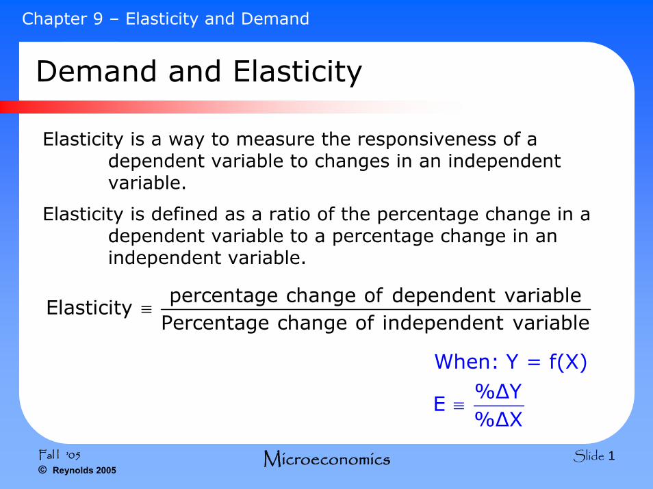
Demand and Elasticity
Elasticity is a way to measure the responsiveness of a dependent variable to changes in an independent variable.
Elasticity is defined as a ratio of the percentage change in a dependent variable to a percentage change in an independent variable.
percentage change of dependent variableElasticity
Percentage change of independent variable≡
When: Y = f(X)%ΔY
E%ΔX
≡
Fal l ’05© Reynolds 2005
Microeconomics Slide 2
Chapter 9 – Elasticity and Demand
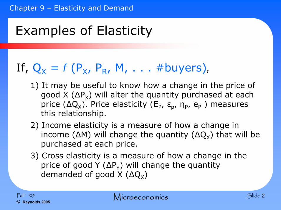
If, QX = f (PX, PR, M, . . . #buyers),
1) It may be useful to know how a change in the price of good X (ΔPX) will alter the quantity purchased at each price (ΔQX). Price elasticity (EP, εp, ηP, eP ) measures this relationship.
2) Income elasticity is a measure of how a change in income (ΔM) will change the quantity (ΔQX) that will be purchased at each price.
3) Cross elasticity is a measure of how a change in the price of good Y (ΔPY) will change the quantity demanded of good X (ΔQX)
Examples of Elasticity
Fal l ’05© Reynolds 2005
Microeconomics Slide 3
Chapter 9 – Elasticity and Demand
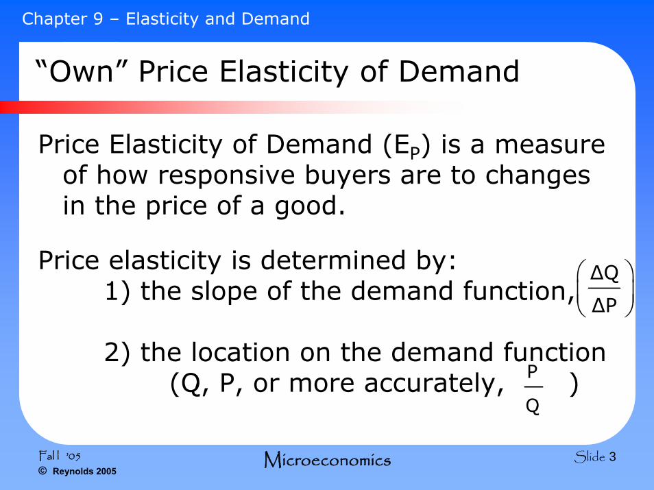
“Own” Price Elasticity of Demand
Price Elasticity of Demand (EP) is a measure of how responsive buyers are to changes in the price of a good.
Price elasticity is determined by:1) the slope of the demand function,
2) the location on the demand function (Q, P, or more accurately, )P
Q
ΔQ
ΔP
⎛ ⎞⎜ ⎟⎝ ⎠
Fal l ’05© Reynolds 2005
Microeconomics Slide 4
Chapter 9 – Elasticity and Demand
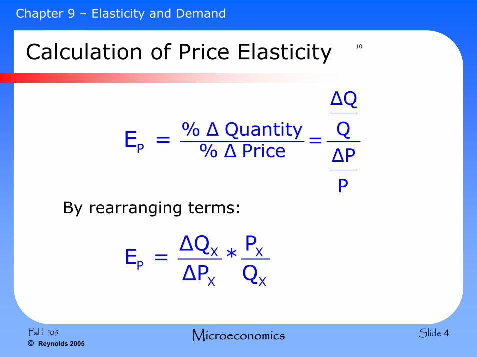
Calculation of Price Elasticity 10
P% Δ Quantity
% Δ Price
ΔQ
QΔP
P
=E =
By rearranging terms:
X XP
X X
ΔQ PE = *
ΔP Q
Fal l ’05© Reynolds 2005
Microeconomics Slide 5
Chapter 9 – Elasticity and Demand
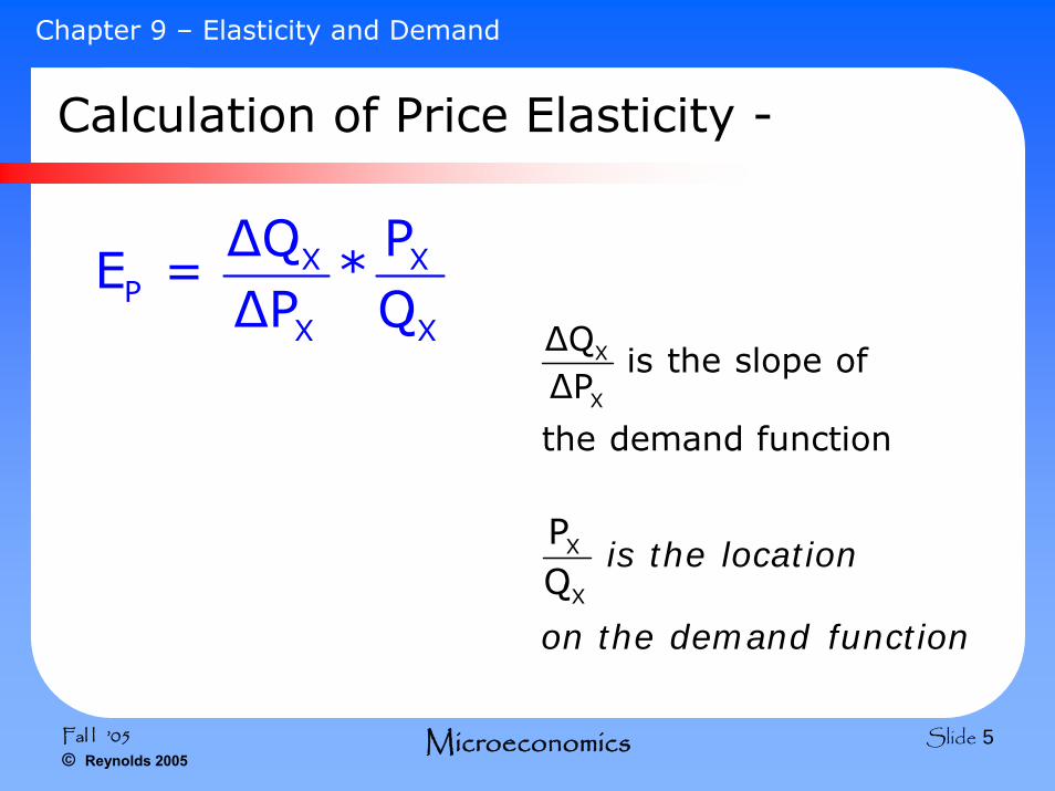
X XP
X X
ΔQ PE = *
ΔP Q
Calculation of Price Elasticity -
X
X
ΔQis the slope of
ΔP
the demand function
X
X
PQ
is the location
on the demand function
Fal l ’05© Reynolds 2005
Microeconomics Slide 6
Chapter 9 – Elasticity and Demand
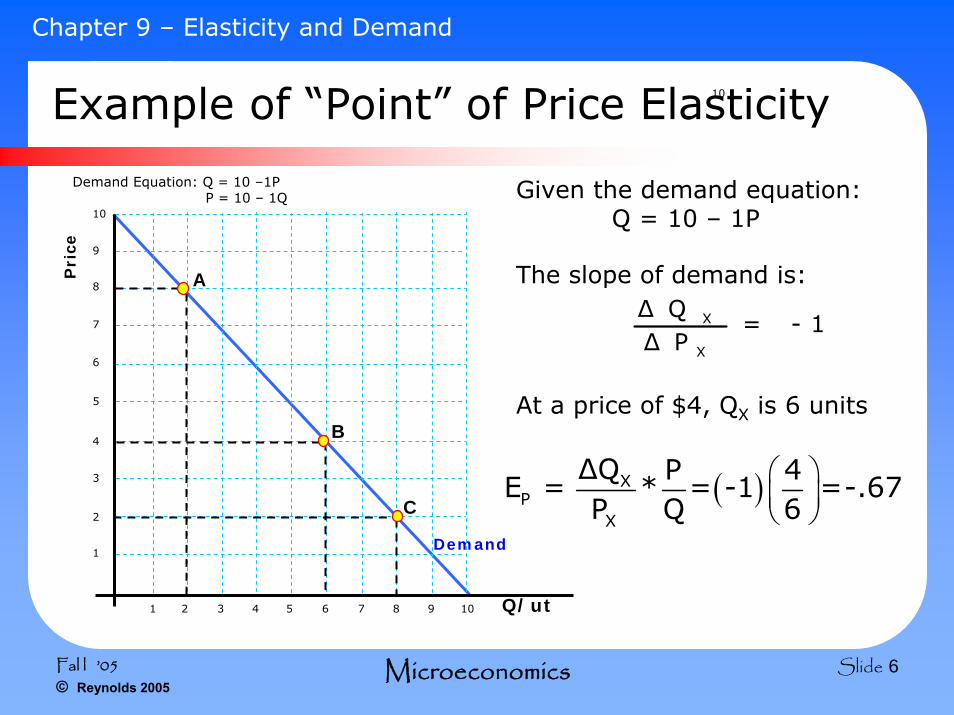
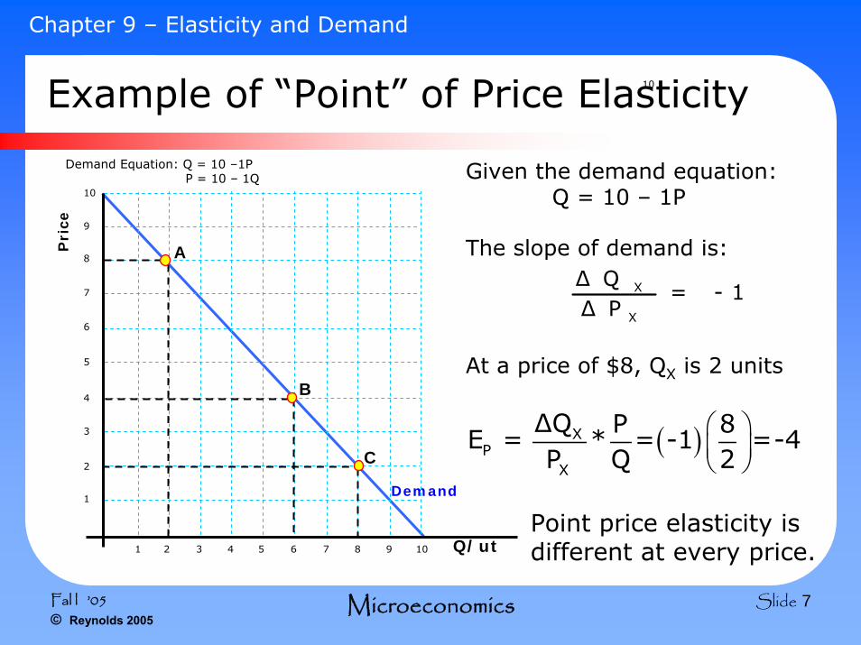
Example of “Point” of Price Elasticity10
Demand Equation: Q = 10 –1PP = 10 – 1Q
10987654321
Demand
Q/ut
Pri
ce
1
2
3
4
5
6
7
9
8
10
A
B
C
Given the demand equation:Q = 10 – 1P
The slope of demand is:
At a price of $4, QX is 6 units
X
X
Δ Q= - 1
Δ P
( )XP
X
ΔQ P 4E = * = -1 =-.67
P Q 6⎛ ⎞⎜ ⎟⎝ ⎠
Fal l ’05© Reynolds 2005
Microeconomics Slide 7
Chapter 9 – Elasticity and Demand
Example of “Point” of Price Elasticity10
Demand Equation: Q = 10 –1PP = 10 – 1Q
10987654321
Demand
Q/ut
Pri
ce
1
2
3
4
5
6
7
9
8
10
A
B
C
Given the demand equation:Q = 10 – 1P
The slope of demand is:
At a price of $8, QX is 2 units
X
X
Δ Q= - 1
Δ P
( )XP
X
ΔQ P 8E = * = -1 =-4
P Q 2⎛ ⎞⎜ ⎟⎝ ⎠
Point price elasticity is different at every price.
Fal l ’05© Reynolds 2005
Microeconomics Slide 8
Chapter 9 – Elasticity and Demand
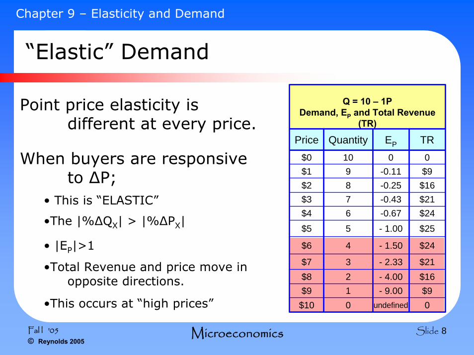
Q = 10 – 1PDemand, EP and Total Revenue
(TR)
Price Quantity EP TR$0 10 0 0$1 9 -0.11 $9$2 8 -0.25 $16$3 7 -0.43 $21$4 6 -0.67 $24$5 5 - 1.00 $25
$6 4 - 1.50 $24
$7 3 - 2.33 $21$8 2 - 4.00 $16$9 1 - 9.00 $9
$10 0 undefined 0
“Elastic” Demand
Point price elasticity is different at every price.
When buyers are responsive to ΔP;
• This is “ELASTIC”
•The |%ΔQX| > |%ΔPX|
• |EP|>1
•Total Revenue and price move in opposite directions.
•This occurs at “high prices”
Fal l ’05© Reynolds 2005
Microeconomics Slide 9
Chapter 9 – Elasticity and Demand
Q = 10 – 1PDemand, EP and Total Revenue
(TR)
Price Quantity EP TR$0 10 0 0$1 9 -0.11 $9$2 8 -0.25 $16$3 7 -0.43 $21$4 6 -0.67 $24$5 5 - 1.00 $25
$6 4 - 1.50 $24
$7 3 - 2.33 $21$8 2 - 4.00 $16$9 1 - 9.00 $9
$10 0 undefined 0
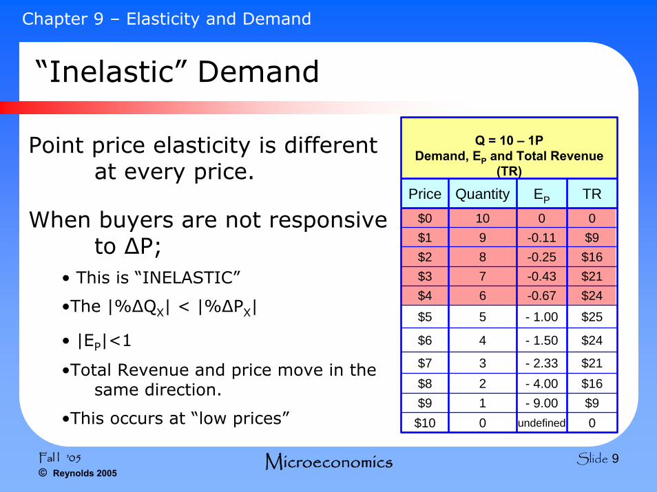
“Inelastic” Demand
Point price elasticity is different at every price.
When buyers are not responsive to ΔP;
• This is “INELASTIC”
•The |%ΔQX| < |%ΔPX|
• |EP|<1
•Total Revenue and price move in the same direction.
•This occurs at “low prices”
Fal l ’05© Reynolds 2005
Microeconomics Slide 10
Chapter 9 – Elasticity and Demand
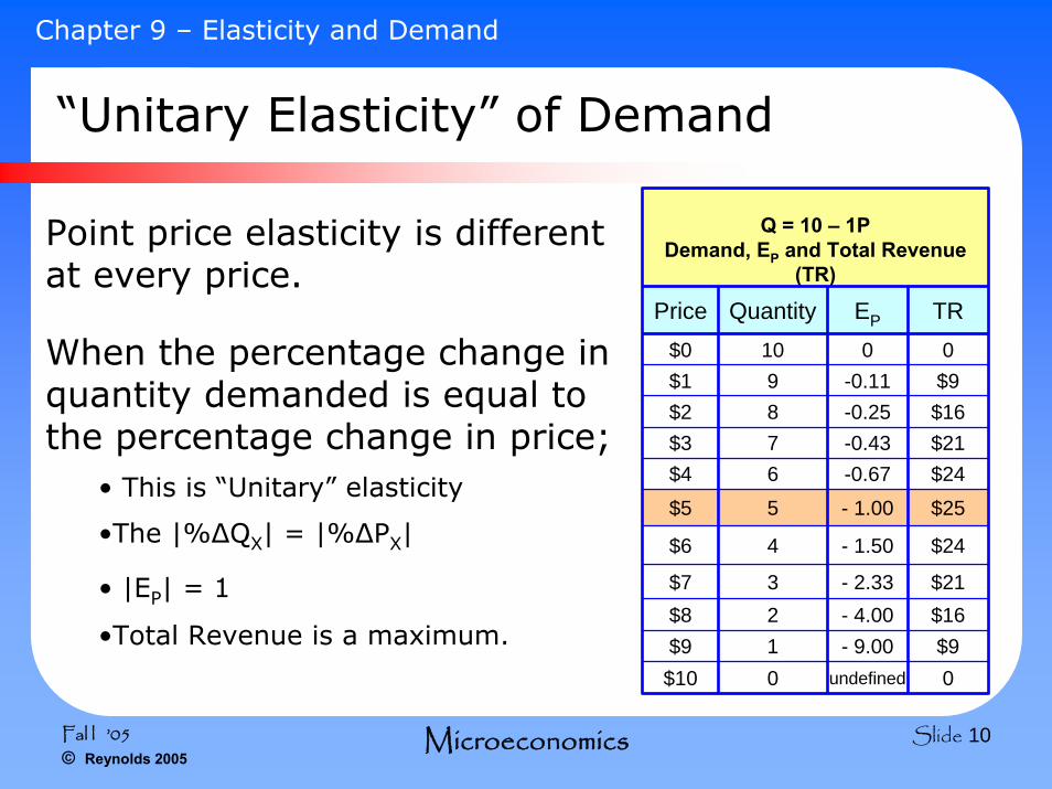
Q = 10 – 1PDemand, EP and Total Revenue
(TR)
Price Quantity EP TR$0 10 0 0$1 9 -0.11 $9$2 8 -0.25 $16$3 7 -0.43 $21$4 6 -0.67 $24$5 5 - 1.00 $25
$6 4 - 1.50 $24
$7 3 - 2.33 $21$8 2 - 4.00 $16$9 1 - 9.00 $9
$10 0 undefined 0
“Unitary Elasticity” of Demand
Point price elasticity is different at every price.
When the percentage change in quantity demanded is equal to the percentage change in price;
• This is “Unitary” elasticity
•The |%ΔQX| = |%ΔPX|
• |EP| = 1
•Total Revenue is a maximum.
Fal l ’05© Reynolds 2005
Microeconomics Slide 11
Chapter 9 – Elasticity and Demand
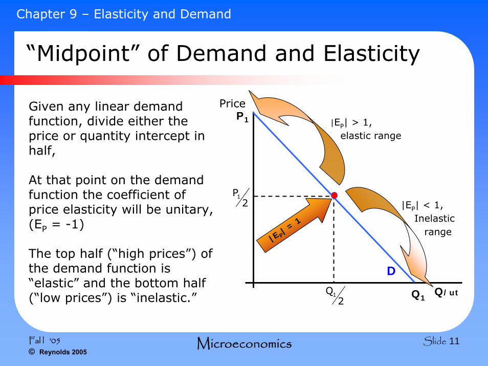
“Midpoint” of Demand and Elasticity
Given any linear demand function, divide either the price or quantity intercept in half,
At that point on the demand function the coefficient of price elasticity will be unitary,(EP = -1)
The top half (“high prices”) of the demand function is “elastic” and the bottom half (“low prices”) is “inelastic.”
|EP| =
1
D
|EP| < 1, Inelastic
range
|EP| > 1, elastic range
Price
Q/ut
P1
1P2
Q11Q2
Fal l ’05© Reynolds 2005
Microeconomics Slide 12
Chapter 9 – Elasticity and Demand
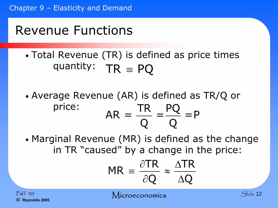
Revenue Functions
• Total Revenue (TR) is defined as price times quantity: TR PQ≡
• Average Revenue (AR) is defined as TR/Q or price: TR PQ
AR = = =PQ Q
• Marginal Revenue (MR) is defined as the change in TR “caused” by a change in the price:
TR TRMR
Q Q∂ Δ
≡ ≈∂ Δ
Fal l ’05© Reynolds 2005
Microeconomics Slide 13
Chapter 9 – Elasticity and Demand
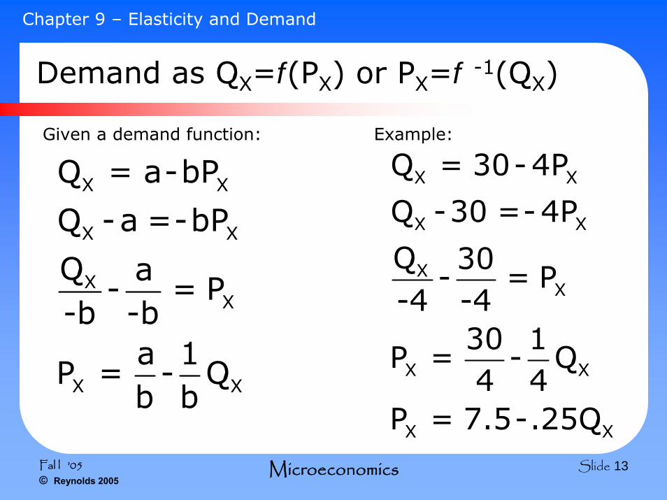
Demand as QX=f(PX) or PX=f -1(QX)
Given a demand function:
X X
X X
XX
X X
Q = a-bP
Q -a =-bP
Q a- = P
-b -ba 1
P = - Qb b
X X
X X
XX
X X
X X
Q = 30-4P
Q -30 =-4P
Q 30- = P
-4 -430 1
P = - Q4 4
P = 7.5-.25Q
Example:
Fal l ’05© Reynolds 2005
Microeconomics Slide 14
Chapter 9 – Elasticity and Demand
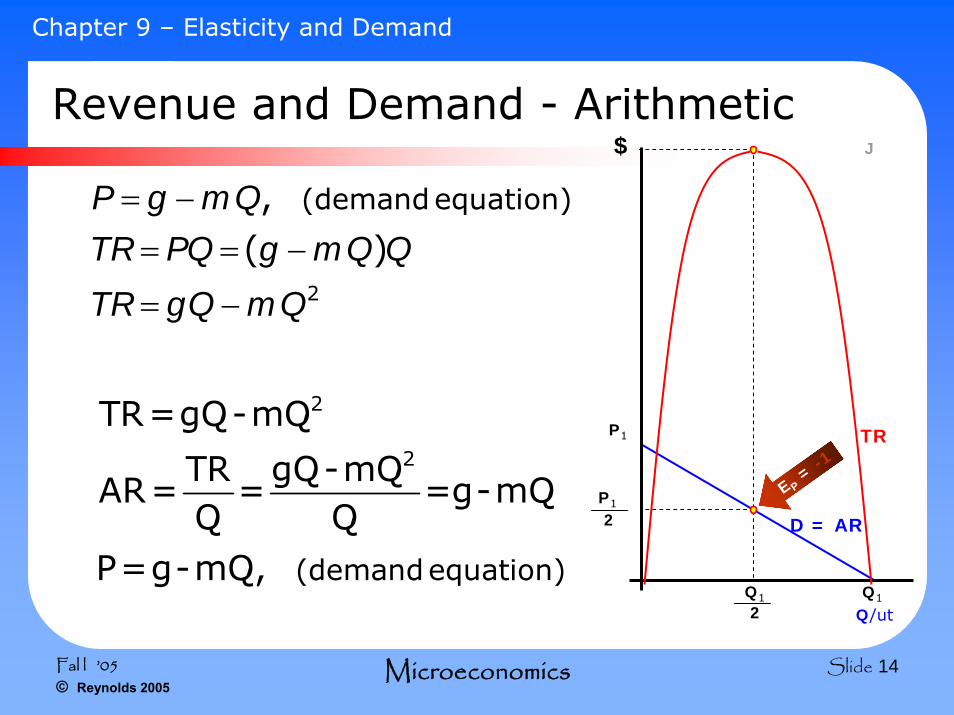
Revenue and Demand - Arithmetic
2
(demandequation),( )
P g mQTR PQ g mQ Q
TR gQ mQ
= −= = −
= −
2
2
(demandequation)
TR=gQ-mQ
TR gQ-mQAR= = =g-mQ
Q QP=g-mQ,
Q1
J
D = AR
Q/ut
$
Q1
2
P1
P1
2
TR
E P=
-1
Fal l ’05© Reynolds 2005
Microeconomics Slide 15
Chapter 9 – Elasticity and Demand
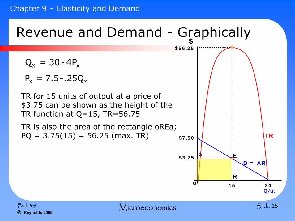
Revenue and Demand - Graphically
X XQ = 30-4P
X XP = 7.5-.25Q
TR for 15 units of output at a price of $3.75 can be shown as the height of the TR function at Q=15, TR=56.75
TR is also the area of the rectangle oREa; PQ = 3.75(15) = 56.25 (max. TR)
D = AR
Q/ut
$
TR$7.50
3015
$3.75
$56.25
a
oR
E
Fal l ’05© Reynolds 2005
Microeconomics Slide 16
Chapter 9 – Elasticity and Demand
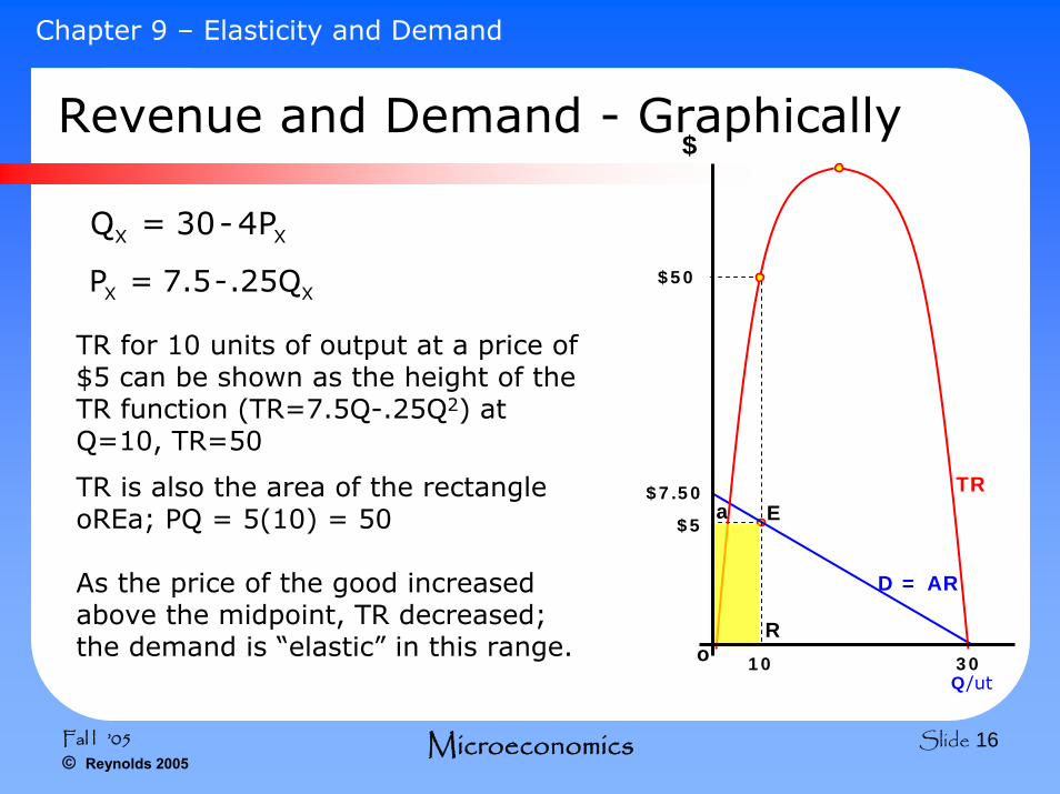
Revenue and Demand - Graphically
X XQ = 30-4P
X XP = 7.5-.25Q
a
TR for 10 units of output at a price of $5 can be shown as the height of the TR function (TR=7.5Q-.25Q2) at Q=10, TR=50
TR is also the area of the rectangle oREa; PQ = 5(10) = 50
As the price of the good increased above the midpoint, TR decreased; the demand is “elastic” in this range.
D = AR
Q/ut
$
TR
3010
$7.50
$5
$50
oR
E
Fal l ’05© Reynolds 2005
Microeconomics Slide 17
Chapter 9 – Elasticity and Demand
Revenue and Demand - Graphically
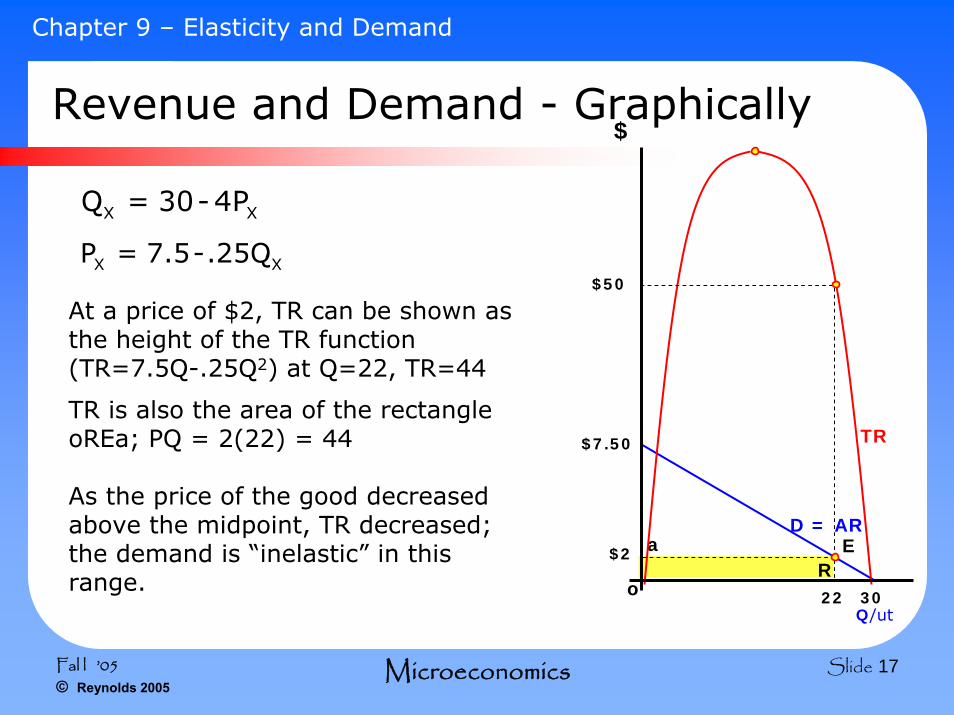
X XQ = 30-4P
X XP = 7.5-.25Q
a
At a price of $2, TR can be shown as the height of the TR function (TR=7.5Q-.25Q2) at Q=22, TR=44
TR is also the area of the rectangle oREa; PQ = 2(22) = 44
As the price of the good decreased above the midpoint, TR decreased; the demand is “inelastic” in this range.
$7.50
o 30Q/ut
TR
D = AR
$
22
$2
$50
RE
Fal l ’05© Reynolds 2005
Microeconomics Slide 18
Chapter 9 – Elasticity and Demand
Revenue and Demand - Table
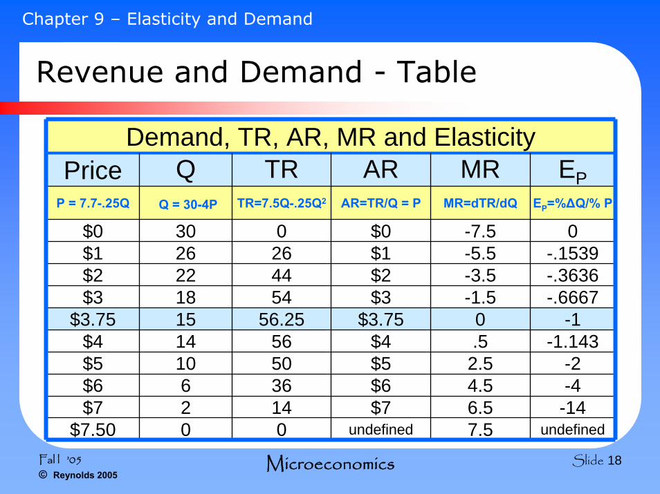
Demand, TR, AR, MR and ElasticityPrice Q TR AR MR EP
P = 7.7-.25Q Q = 30-4P TR=7.5Q-.25Q2 AR=TR/Q = P MR=dTR/dQ EP=%ΔQ/% P
$0 30 0 $0 -7.5 0$1 26 26 $1 -5.5 -.1539$2 22 44 $2 -3.5 -.3636$3 18 54 $3 -1.5 -.6667
$3.75 15 56.25 $3.75 0 -1$4 14 56 $4 .5 -1.143
$7.50 0 0 undefined 7.5 undefined
$5 10 50 $5 2.5 -2$6 6 36 $6 4.5 -4$7 2 14 $7 6.5 -14
Fal l ’05© Reynolds 2005
Microeconomics Slide 19
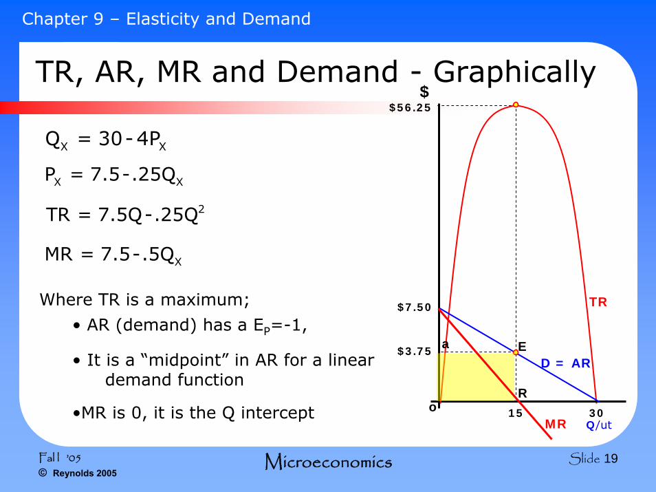
Chapter 9 – Elasticity and Demand
TR, AR, MR and Demand - Graphically
X XQ = 30-4P
X XP = 7.5-.25Q
Where TR is a maximum;
• AR (demand) has a EP=-1,
• It is a “midpoint” in AR for a linear demand function
•MR is 0, it is the Q intercept
D = AR
Q/ut
$
TR$7.50
3015
$3.75
$56.25
a
oR
E
MR
2TR = 7.5Q-.25Q
XMR = 7.5-.5Q
Fal l ’05© Reynolds 2005
Microeconomics Slide 20
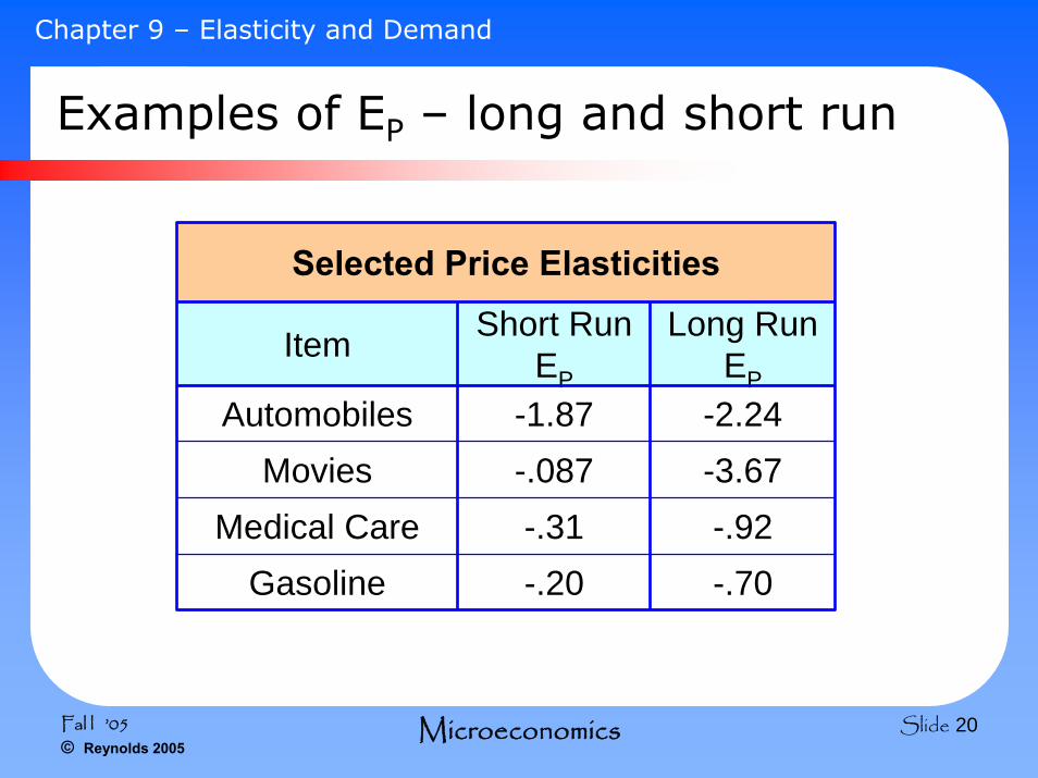
Chapter 9 – Elasticity and Demand
Selected Price Elasticities
Item Short Run EP
Long Run EP
Automobiles -1.87 -2.24Movies -.087 -3.67
Medical Care -.31 -.92Gasoline -.20 -.70
Examples of EP – long and short run
Fal l ’05© Reynolds 2005
Microeconomics Slide 21
Chapter 9 – Elasticity and Demand
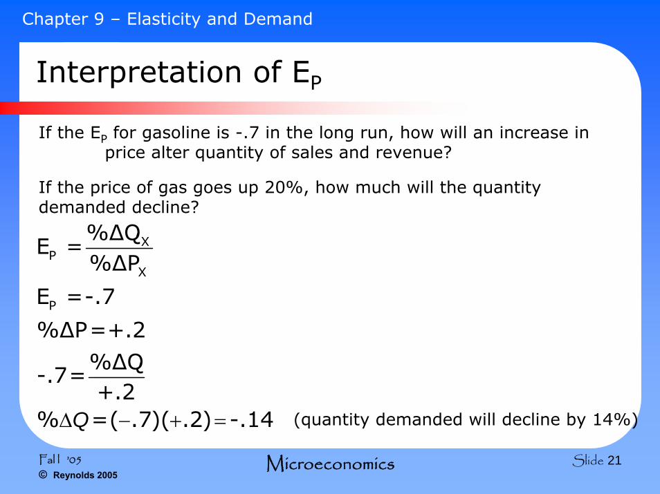
Interpretation of EP
If the EP for gasoline is -.7 in the long run, how will an increase in price alter quantity of sales and revenue?
If the price of gas goes up 20%, how much will the quantity demanded decline?
XP
X
P
%ΔQE =
%ΔP
E =-.7
%ΔP=+.2%ΔQ
-.7=+.2
% =( .7)( .2) -.14QΔ − + = (quantity demanded will decline by 14%)
Fal l ’05© Reynolds 2005
Microeconomics Slide 22
Chapter 9 – Elasticity and Demand
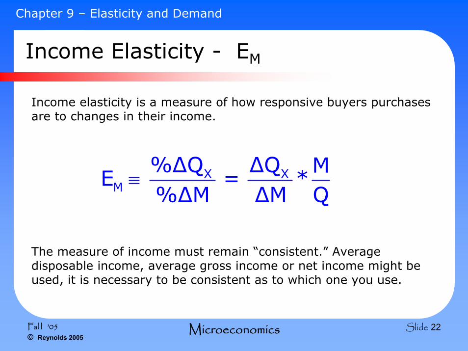
Income Elasticity - EM
Income elasticity is a measure of how responsive buyers purchases are to changes in their income.
X XM
%ΔQ ΔQ ME = *
%ΔM ΔM Q≡
The measure of income must remain “consistent.” Average disposable income, average gross income or net income might be used, it is necessary to be consistent as to which one you use.
Fal l ’05© Reynolds 2005
Microeconomics Slide 23
Chapter 9 – Elasticity and Demand
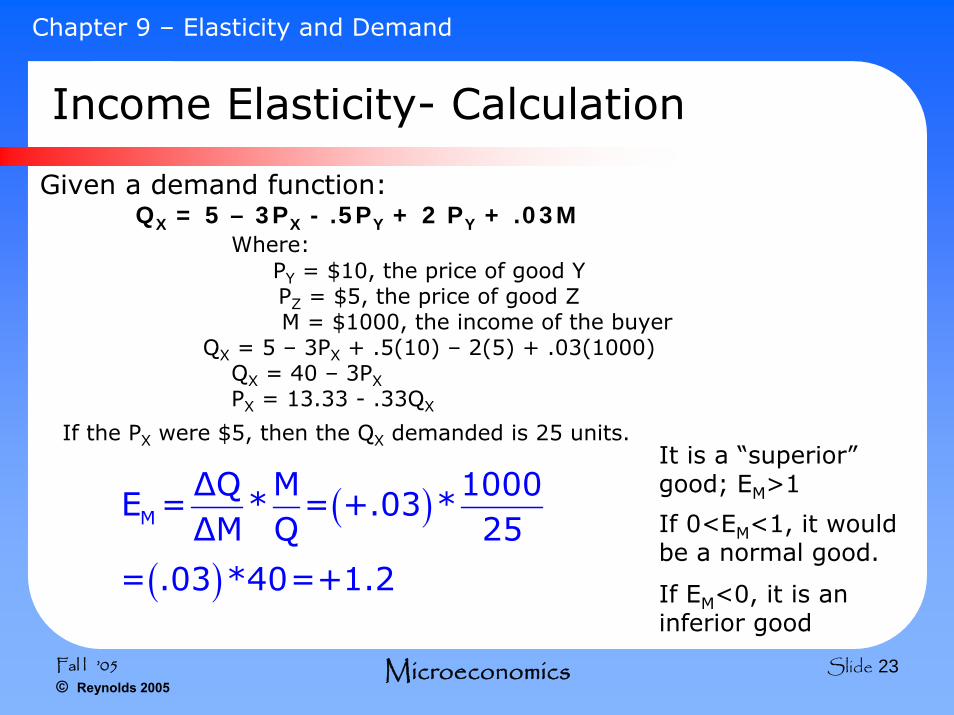
Given a demand function:QX = 5 – 3PX - .5PY + 2 PY + .03M
Where:PY = $10, the price of good YPZ = $5, the price of good ZM = $1000, the income of the buyer
QX = 5 – 3PX + .5(10) – 2(5) + .03(1000)QX = 40 – 3PXPX = 13.33 - .33QX
Income Elasticity- Calculation
If the PX were $5, then the QX demanded is 25 units.
( )
( )
M
ΔQ M 1000E = * = +.03 *
ΔM Q 25
= .03 *40=+1.2
It is a “superior”good; EM>1
If 0<EM<1, it would be a normal good.
If EM<0, it is an inferior good
Fal l ’05© Reynolds 2005
Microeconomics Slide 24
Chapter 9 – Elasticity and Demand
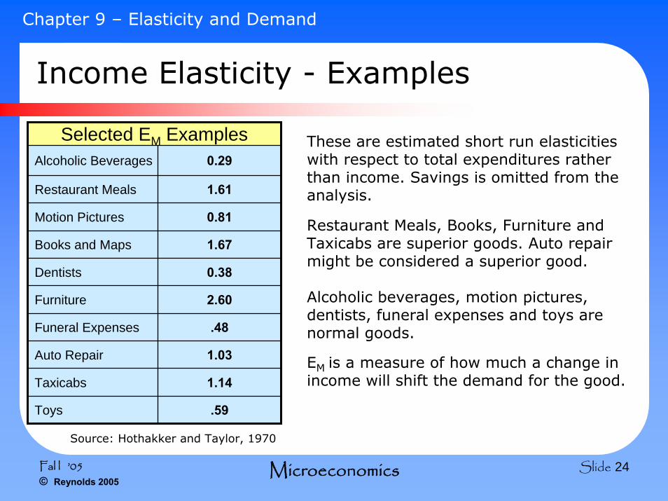
Income Elasticity - Examples
Selected EM ExamplesAlcoholic Beverages 0.29
Restaurant Meals 1.61
Motion Pictures 0.81
Books and Maps 1.67
Dentists 0.38
Furniture 2.60
Funeral Expenses .48
Auto Repair 1.03
Taxicabs 1.14
Toys .59
Source: Hothakker and Taylor, 1970
These are estimated short run elasticitieswith respect to total expenditures rather than income. Savings is omitted from the analysis.
Restaurant Meals, Books, Furniture and Taxicabs are superior goods. Auto repair might be considered a superior good.
Alcoholic beverages, motion pictures, dentists, funeral expenses and toys are normal goods.
EM is a measure of how much a change in income will shift the demand for the good.
Fal l ’05© Reynolds 2005
Microeconomics Slide 25
Chapter 9 – Elasticity and Demand
Income Elasticity - Interpretation
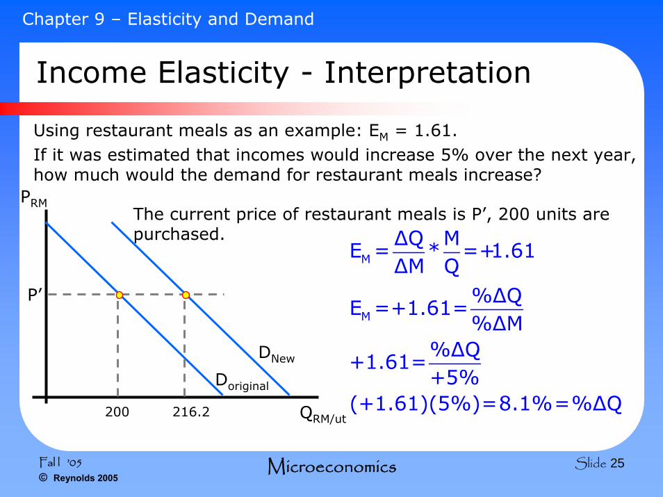
Using restaurant meals as an example: EM = 1.61. If it was estimated that incomes would increase 5% over the next year, how much would the demand for restaurant meals increase?
The current price of restaurant meals is P’, 200 units are purchased.
M
M
ΔQ ME = * =+1.61
ΔM Q%ΔQ
E =+1.61=%ΔM
%ΔQ+1.61=
+5%(+1.61)(5%)=8.1%=%ΔQ
PRM
QRM/ut
Doriginal
P’
200 216.2
DNew
Fal l ’05© Reynolds 2005
Microeconomics Slide 26
Chapter 9 – Elasticity and Demand
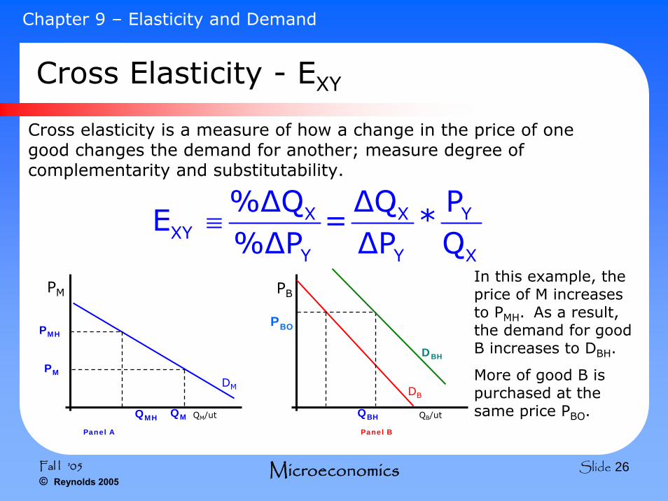
Cross Elasticity - EXY
Cross elasticity is a measure of how a change in the price of one good changes the demand for another; measure degree of complementarity and substitutability.
X X YXY
Y Y X
%ΔQ ΔQ PE = *
%ΔP ΔP Q≡
In this example, the price of M increases to PMH. As a result, the demand for good B increases to DBH.
More of good B is purchased at the same price PBO.QMH QM/ut
PM
DM
QM
PM
PMH
Panel A Panel B
QB/ut
DB
QBH
DBH
PB
PBO
Fal l ’05© Reynolds 2005
Microeconomics Slide 27
Chapter 9 – Elasticity and Demand
Cross Elasticity - EXY
Cross elasticity has been used to identify markets in court cases, e.g. US v. ALCOA-Rome Cable Case (1964), Brown Shoe v. US Case (1962) and US v. Du Pont Cellophane Case (1956).
If EXY > 0 this is evidence that goods X and Y are substitutes (not proof)
If EXY < 0 this is evidence that goods X and Y are complements, (not proof)
EXY is not the same as EYX, Beef may be a better substitute for pork than pork is for beef.
Berndt, Friedlaender and Chaing (1990) estimate the EXY between Ford and GM at 7.01. A 1% increase in the price of Fords will result in a 7% increase in the demand for GM cars.