Demand Determinants for U.S. Processed Food Exports to Emerging/Low and Middle-Income Countries

Authors:

Mary A. Marchant Professor, International Trade

University of Kentucky Agricultural Economics 314 C.E. Barnhart Bldg.

Lexington, KY 40546-0276 Phone: (859) 257-7260 Fax: (859) 257-7290

E-mail: mmarchan@uky.edu

Sanjeev Kumar Research Assistant

University of Kentucky Agricultural Economics 331 C.E. Barnhart Bldg.

Lexington, KY 40546-0276 Phone: (859) 257-7272 ext.271

Fax: (859) 257-7290 E-mail: skuma0@uky.edu

Selected Paper prepared for presentation at the American Agricultural Economics Association Annual Meeting, Denver, Colorado, August 1-4, 2004

Copyright 2004 by Mary A. Marchant, and Sanjeev Kumar. Mary A. Marchant is a Professor and Sanjeev Kumar is a Research Assistant in the Department of Agricultural Economics at the University of Kentucky. All rights reserved. Readers may make verbatim copies of this document for non-commercial purposes by any means, provided that this copyright notice appears on all such copies.

Demand Determinants for U.S. Processed Food Exports to

Emerging/Low and Middle-Income Countries

Abstract Because processed foods are the fastest growing segment of U.S. agricultural exports, it is imperative to understand the underlying factors behind this growth. The overall objective of this research is to examine demand for processed foods by low and middle-income countries and assess demand determinants and potential import growth. To achieve this objective, a “modified gravity model” is estimated for U.S. exports of processed foods to 10 low and middle-income countries from 1980-2002 using both classical linear regression and fixed effects approaches. Results indicate that population, income, level of urbanization and an open trade regime have a positive effect on demand for processed foods by low and middle-income countries. As expected, exchange rates and distance have an inverse relationship with imports. Empirical results from the fixed-effects model are similar, with the exception of population. A cross-country comparative analysis of leading potential markets for U.S. processed food exports over the years 2003-2012 concluded that Mexico, China and Brazil respectively are likely to be the three largest future markets for U.S. processed foods among the 10 emerging countries.

Demand Determinants for U.S. Processed Food Exports to Emerging/Low and Middle-Income Countries

The United States is the world’s largest food exporting country and processed

foods are the fastest growing sector of both U.S. agricultural exports and global food

trade. Historically, bulk commodities accounted for the majority of U.S. agricultural

exports. However, U.S. processed foods surpassed bulk goods in export value in 1991

(figure 1). This growth in processed food exports can be ascribed to growing demands in

East Asia and North America, where incomes are rising, diets are diversifying, and, in the

case of some East Asian markets, production capacity is constrained (USDA). Bulk

commodity exports comprised nearly 70 % ($28 billion) of the total value of U.S.

agricultural exports in 1980 but steadily declined to 35 % ($19 billion) in 2002 (USDA-

ERS, 2003). During the same period, processed foods’ share of total agricultural exports

climbed to 65 %. Thus, processed food products1 are the growth market for U.S.

agricultural exports.

The global population is projected to increase by more than 1.2 billion between

1998 and 2018, and almost all of this growth will occur in low and middle-income

countries (Regmi, et al., 2001). In terms of potential U.S. export markets, low and

middle-income countries (see appendix A for the definition of low and middle-income

countries) like China, India, Indonesia, Brazil, Mexico, Thailand, Turkey, Egypt,

Argentina and Malaysia are among the most populous countries in the world, and many

1 The food processing industry includes firms and their establishments that manufacture or process foods and beverages for human consumption and other related products. Examples of processed and consumer-ready foods used in this analysis include meats and meat products; poultry meats; dairy products; fats, oils, and greases; fresh fruits; dried, canned, and frozen fruits; fruit juice including frozen; nuts and nut preparations; fresh vegetables; frozen and canned vegetables; and oilseed products.

1

of their economies are among the fastest growing. Figure 2 describes U.S. agricultural

exports by region. Asia, followed by Latin America, is the largest market for U.S.

agricultural exports. China, Mexico, Thailand, Indonesia, Turkey and Egypt (ERS, 2003)

also ranked among the top twelve markets for U.S. agricultural exports in 2003.

U.S. Agricultural Exports Bulk vs High-Value

0

10,000

20,000

30,000

40,000

1976

1979

1982

1985

1988

1991

1994

1997

2000

Years

US

$ M

n.Bulk

High-Value

Figure 1. Value of U.S. agricultural exports in million U.S. $ for bulk and high value

commodities, 1975-2000 (USDA-ERS, 2003).

Figure 2. U.S. Agricultural Exports in million U.S. $ to 7 World Regions for 1999-

2003 (FATUS, 2003).

2

A new research report prepared for the Goldman Sachs predicts that the combined

economies of Brazil, Russia, China and India could be larger than the G-6 economies in

less than 40 years (Wilson and Purushothaman). Furthermore, multinational food giant

Nestle expects that by 2010 an additional 935 million Asians, many of them Chinese, will

attain a purchasing power of nearly U.S. $1,800 a year. Many of these Asians will move

to urban areas and their “protein’s source will be processed foods” (Hilsenrath).

U.S. Exports of Processed Foods to 5 Asian Countries

0

100

200

300

400

500

600

1980

1982

1984

1986

1988

1990

1992

1994

1996

1998

2000

2002

Years

US

$ M

n

ChinaIndiaMalaysiaThailandIndonesia

U.S. Exports of Processed Foods to 5 Latin America and Middle-East Countries

0500

1000150020002500300035004000

1980

1982

1984

1986

1988

1990

1992

1994

1996

1998

2000

2002

Years

US

$ M

n

EgyptTurkeyMexicoArgentinaBrazil

Figure 3. U.S. Processed Food Exports in Million U.S. $ to 10 Emerging Markets for

years 1980-2002 (FATUS, 2003).

3

Research Objectives

The overall objective of this research is to examine demand for processed foods

by low and middle-income countries, seeking to assess demand determinants and

potential import growth for U.S. processed food exports. In addition to size and distance

(the usual gravity variables), the impact of tariffs, urbanization and exchange rates on

import demand for processed foods will be analyzed using an augmented gravity model.

The overall objective was achieved by completing the following tasks:

1. Collect data on demand determinants for processed foods by the ten countries.

Examples of consumption data include income, tastes and preferences, population and

level of urbanization. Countries examined include Brazil, Argentina, Mexico,

Thailand, Indonesia, Malaysia, China, India, Egypt and Turkey.

2. Analyze the trade regimes of these countries, e.g., degree of trade liberalization.

3. Develop an import demand model for U.S. exports of processed foods.

4. Conduct cross-country comparisons by using the results of the above model to map

out potential future demand by these countries and rank the potentially lucrative

markets for U.S. processed food exports.

Literature Review

Recent Trends in Processed Food Trade

Global food consumption patterns were transformed during the past decade due to

increased urbanization, demographic shifts, higher incomes, improved transportation

facilities, and consumer awareness of food quality and safety (Regmi, 2001). In

developing countries, better retail facilities, paucity of time, and higher purchasing power

among urban dwellers have changed eating habits and spurred demand for processed

4

foods. In addition, the urban population in developing countries is expected to double to

nearly 4 billion people by 2020 (Regmi and Dyck, 2001). This population growth will

create a huge potential market for U.S. exports of processed foods (Regmi, 2001).

Consumers in middle-income and, especially, low-income countries spend a

greater portion of their budget on staple food products (e.g. cereals) and are more

responsive to changes in food prices and incomes (Gelhar and Coyle, 2001). However,

this response differs across food items. For example, when prices and incomes change,

consumers in low and middle-income countries make few adjustments to their staple food

budgets relative to higher value food items (e.g. dairy and meat). Such changes have

spurred global agricultural trade and altered its composition between bulk and processed

foods. However, the impact of income growth in developed and developing countries on

trade patterns is not similar (Regmi, 2001).

The Gravity Model

One of the most popular models used to estimate international trade flows is the

gravity model. This model, developed by Tinbergen and Poyhonen in the early 1960s, is

described as the “workhorse for empirical studies of the pattern of trade” (Bayoumi and

Eichengreen, p. 142, 1997) and the “standard empirical framework used to predict how

countries match up in international trade” (Rauch, p.10, 1999). The “formal theoretical

foundations” of the gravity model for empirical studies of international trade are provided

by Anderson, Krugman, Helpman and Bergstrand, and “are now well-established” (Baier

and Bergstrand, 2001).

Gravity equations are log-linear, cross-sectional specifications that estimate

nominal bilateral trade flow values between two countries (Baier and Bergstrand, 2001).

5

Bilateral trade flows follow the “physical principles of gravity” where two opposite

forces - income and impediments to trade – determine the volume of bilateral trade

(Fontagné and Pasteels). Impediments to trade include transportation costs, trade policies,

uncertainty, cultural differences, and limited overlap in consumer preferences (Fontagné

and Pasteels). The standard gravity model predicts that “countries with similar levels of

output per capita will trade more than countries will dissimilar levels” (Frankel, 1997).

Krugman states that gravity equations successfully explain the volume of trade

between two countries using few variables like the GDPs of the two trading countries and

the distance between them. Krugman describes a typical gravity equation as follows:

(1) Tij = kYiα

YjβDij

-γ

where Tij is the volume of trade between countries i and j; Yi and Yj are their respective

GDPs; Dij is the distance between the two countries; and k is a parameter. According to

Krugman, estimation of equation (1) typically results in values of α and β that are one and

a value of γ that is statistically different from zero (i.e. distance has a strong effect on

trade). Frankel, Stein and Wei (1996) also found the effect of log distance on bilateral

trade to be statistically significant.

It is common to add other variables to the basic gravity model. Frankel (1997)

states that other explanatory variables2, such as population to control for the size of the

country and dummy variables representing trading blocks (to evaluate the effect of

preferential trading agreements), are often added. Bergstrand (1985) and Fontagné and

Pasteels also modify the theoretical model to control for various factors such as regional

2 According to Frankel (1997), the effects of economic size (GDP) and population are independent.

6

trade integration and preferential arrangements. Baier and Bergstrand (2001) included

variables representing trade barriers (e.g. transport costs and tariffs) to their model.

Bougheas, Demetriades, and Morgenroth added infrastructure variables to their model

because transport costs are not only a function of distance but also roads, ports, and

telecommunication networks. Exchange rates (ER) are also included to proxy price and

inflation (Bergstrand, 1985; Fontagné and Pasteels).

A modified gravity model, therefore, estimates the value of bilateral trade using

variables representing GDP, population as a measure of the size of the market, trade

impediments, and enhancement factors. Generally, a gravity equation estimates bilateral

trade flows, but it may also be used to estimate the determinants of the volume of trade

(Fontagné and Pasteels). Likewise, this research seeks to estimate the determinants of the

volume of U.S. exports using a gravity equation.

Determinants of Food Trade

Coyle et al. (1998) examined the major determinants of changes in the structure of

global food trade and identified income growth, food expenditures, factors of production,

transport costs, and trade policy changes as key economic factors that explain shifts in

trade patterns. They concluded that growth in income impacts food consumption more

than any other factor. Gehlhar and Coyle (2001) found that that improved diet in

developing countries, resulting from income growth, has contributed to changes in global

trade patterns. However, the connection between changes in food consumption patterns

and changes in world agricultural trade goes beyond income growth and dietary changes.

The global population is expected to increase by 1.2 billion people between 1998

and 2018. This expected growth in population (SZ) and rising incomes in developing

7

countries are likely to account for most of the increase in global food demand over the

next twenty years (Regmi, Deepak, Seale, and Bernstein, 2001). Lifestyle improvements

are concurrent to rising levels of urbanization and result in greater emphasis on

convenience and higher food consumption away from home.

Transport costs (DIS) are barriers to trade that vary by commodity. Transportation

costs for processed foods are high owing to the perishable nature of many commodities

(Gehlhar and Coyle, 2001). A reduction in overall transportation costs owing to better

transportation technology will increase trade in processed foods (Regmi and Gelhar,

2001). Feenstra found that about two-fifths of trade growth relative to income is

explained by the combined effect of declining transport costs and falling tariffs: the latter

accounting for twice as much as the former. Transport costs are usually proxied by the

distance between importing and exporting countries.

Trade Policy, Tariffs and Openness Index

High protection of agricultural commodities in the form of tariffs continues to be

a barrier to world trade. Some countries provide unfair protection for certain domestic

products by imposing high duties on comparable imported goods that result in higher

prices for imported goods. The global average tariff on agricultural products is 62 %

(Gibson et al.) and accounts for 52 % of the increase in world prices (Burfisher et al.).

Although both developed and developing countries impose high tariffs, average

agricultural tariffs in developing countries are much higher. Average commodity tariffs

range from 50 to 91 %, with tobacco, meats, dairy, sugar, and sweeteners subject to the

highest tariff rates (Gibson et al.). Reduction in tariffs will make certain food items more

affordable in developing countries (Gehlhar and Coyle, 2001) and expand agricultural

8

trade. The average tariff for the U.S. (12 %) is one of the lowest in the world. Therefore,

U.S. agriculture stands to gain from global tariff reductions (Gibson et al.).

Membership in the World Trade Organization (WTO) is crucial in determining

the tariff levels of importing countries. Two significant accomplishments of the WTO are

the extension of trading concessions by member states to one another and market access

for agricultural goods by introducing “tariffication” (dell’Aquila, Sarker and Meilke ).

Identification of potentially lucrative markets for U.S. processed food exports depends

crucially on the prospects of trade liberalization by WTO members.

Krugman attributes the growth in world trade since 1950 to political causes.

Specifically, recent growth is a response to the removal of protectionist measures and the

lowering of tariffs that have restricted trade since 1913. Growth is not due to the

commonly held journalistic view of technology-led reductions in transportation costs.

Baier and Bergstrand (2001) concur with Krugman and concluded that income growth

contributed 67 %, tariff-rate reductions 25 %, and transport-cost reductions 8 % to the

real growth of world merchandise trade among several OECD countries between the late

1950s and late 1980s. According to Athukorala and Sen, inter-country differences in

processed food exports’ growth rates are influenced more by trade policy regime (TRAD)

than by resource endowments. While resource availability is essential, exports of

processed foods depend crucially on the “openness” of domestic trade policy.

Clearly, tariff rates and trade policies have a significant impact on international

trade. Given the importance of trade policy to a country’s propensity to import, trade

regimes are significant in identifying the most lucrative future markets for U.S. exports of

processed foods. However, it is difficult to quantify protectionism owing to different

9

tariff rates applied to different commodities (Krugman) and the complex nature of

commercial policies.

Edwards states that many variables, including tariffs, licenses, quotas,

prohibitions and exchange controls, impact international trade. Attempts to measure trade

orientation by a single indicator may be an exercise in futility or result in omitted variable

error. Comparative measures of openness are also imperfect. Edwards cites other authors

who state that South Korea is an open and outward-oriented economy for some, but for

others it is semi-closed and government-controlled.

Sachs and Warner conducted a comprehensive study of the process of global

integration and assessed its effects on the economic growth of reforming countries. They

used cross-country indicators of trade openness or liberalization to classify each

country’s orientation to the global economy as “open” or “closed” and determined the

year of trade liberalization, if at all. However, Edwards points out that this categorization

of a trade regime as “open” or “closed” is a binary classification, which does not account

for varying degrees of government intervention.

Theoretical Model

This research employs a variation of the cross-sectional gravity methodology

discussed above to model the relationship between U.S. exports of processed foods and

the variables that determine demand for such foods. Following Frankel (1997) and

Bergstrand (1985), variables other than the “usual gravity variables” have been included

to capture the impact of trade regime and urbanization on demand for U.S. exports.

Following Summary, the theoretical model for our research is a gravity-type equation that

10

estimates “one-way” trade, in our case, U.S. exports. The gravity model used in this

investigation is defined as equation (2).

(2) EXPitus = f (SZit, GDPit, ERit, DISi, TRADit, URBit) + εit

In equation (2), EXPitus is U.S. exports of processed foods to importing country i in time

t, SZ is the population of importing country i, GDP is the gross domestic product of

country i, ER is the exchange rate of country i in local currency per U.S. dollar, DIS is the

distance between the U.S. and the importing country i, TRAD is the trade regime of

country i, URB is the level of urbanization in country i, and ε is a stochastic error term.

Using equation (2), the following hypotheses are tested:

1) Population is positively related to imports (i.e., as population increases, demand

for processed foods increases);

2) GDP is positively related to imports (i.e., as GDP increases, demand for processed

foods also increases);

3) Exchange rates are negatively related to imports (i.e., an appreciation of the U.S.

dollar, which occurs when more of a local currency is needed to buy a U.S. dollar,

causes a decrease in demand for U.S. exports of processed foods by the importing

country);

4) Distance is negatively related to imports (i.e., as distance between exporting and

importing countries increases, demand for U.S. processed foods decreases);

5) Trade regime is positively related to imports (i.e., as a trade regime becomes

“open,” demand for U.S. processed foods increases); and

11

6) Urbanization is positively related to imports (i.e., as the importing country’s level

of urbanization increases, demand for U.S. processed foods increases).

Data Description and Methodology

Data on U.S. exports of processed foods (see footnote 1 for a complete list of

processed foods) from 1980 to 2002 (23 years) for ten low and middle-income countries

(China, India, Indonesia, Brazil, Mexico, Thailand, Turkey, Egypt, Argentina and

Malaysia) were obtained from the Foreign Agricultural Trade of the U.S. (FATUS).

Macroeconomic data on GDP and exchange rates for these countries were obtained from

the USDA-ERS website. Following Fontagné and Pasteels, and Bergstrand (2001),

nominal GDP at current exchange rates was used to proxy income of the importing

country. Data on the levels of urbanization were compiled from the United Nations

Population Division’s 2001 World Urbanization Prospects. The shortest navigable

distance between the U.S. and an importing country was measured in nautical miles (see

www.distances.com for details).

Consumer profiles for each importing country’s purchases of processed foods

were constructed based on the following factors: size of urban population, age structure,

percentage of women employed, consumer tastes and preferences, and perceptiveness to

Western foods. However, because the process used to create the profile is ad hoc and

lacks a standard scale of measurement, it was decided that is more appropriate to use

level of urbanization as a proxy for consumer profile.

The variable representing trade regime for each of the ten countries is best

constructed on the basis of a country’s import policy and tariff structure. Unfortunately,

data on tariff rates for processed foods for each of the ten countries over the period

12

studied are not available. Furthermore, tariff rates are not the best measure of a trade

regime’s liberalization. Instead, a method proposed by Sachs and Warner to measure

trade liberalization is used. Sachs and Warner categorized a trade regime as “closed” if at

least one of the following was true:

1) Non-tariff barriers (NTBs) covering 40 % or more of trade;

2) Average tariff rates of 40 % or more;

3) A black market exchange rate that is depreciated by 20 % or more relative to the

official exchange rate, on an average, during the 1970s or the 1980s;

4) A socialist economic system (as defined by Kornai); and

5) A state monopoly of major exports, defined by a score of 4 on the export-

marketing index in a 1994 World Bank study.

Table 1. Year of trade liberalization of each country included in the study, if the country has an open trade policy, and the year that trade regime was opened, based on Sachs-Warner (1995).

Country Trade Policy Year Opened China Closed Never Open India Open 1994 Indonesia Open 1970 Thailand Open Always Open Malaysia Open 1963 Egypt Closed Never Open Turkey Open 1989 Brazil Open 1991 Argentina Open 1991 Mexico Open 1986

Table 1 reports the results of Sachs and Warner for each of the ten countries used

in this study. Note that the results of Sachs and Warner were established in 1994. Also

13

note that the average tariff levied by the ten countries is not identical. Indonesia,

Thailand, and Malaysia are not as “open” as the U.S., but they are more liberalized than

most developing countries (Sachs and Warner). Given that each of the ten countries is

now a member of the WTO, it is assumed that the “open” economies remained so through

the end of the sample period. For Egypt and China, which were they are assigned a

“closed” trade regime for the entire period of the study. Developing countries are not

required to bring their tariff rates into full compliance with WTO regulations until 2005.

Empirical Results

Equation (2) is estimated as a classical linear regression model and also as a

fixed-effects model. Following Frankel (1997), the gravity model is first estimated using

ordinary least-squares (OLS) regression analysis. Frankel (1997) states that trade data

usually contain enough information to obtain reliable estimates for country size,

proximity, and the other variables in the gravity model. Next, the gravity model is

modified to account for country specific fixed-effects. The fixed-effects model is also

estimated using OLS.

The Classical Linear Regression Model

The data used in this study are arranged into a pooled, cross-section and time-

series panel (NT= 230; N= 10 countries and T= 23 years). Following Baier and

Bergstrand (2001), and Frankel (1997), equation (2) is estimated in natural log

specification. The semi-log expression for equation (2), using the relevant independent

variables previously discussed, yields equation (3). Note that in equation (3), all variables

are transformed except the dummy variable for trade regime (TRAD).

14

(3) lnEXPitus

= β0 + β1lnSZit + β2lnGDPit + β3lnERit + β4lnDISi + β5TRADit +

β6lnURBit + εit

All variables and the i and t subscripts are identical to those defined in equation (2). The

difference is that all continuous variables are now natural log transformations. Recall that

i = country 1,…….,10 (China, India, Indonesia, Malaysia, Thailand, Brazil,

Argentina, Mexico, Egypt and Turkey respectively); and

t = years 1,2,………..23 (1980 through 2003).

Equation (3) was estimated using the STATA statistical computer program

(www.stata.com/support/faqs/stat). No multicollinearity was detected among the

variables. The Durbin-Watson test for autocorrelation was conducted and AR (1) was

found to be present. The modified Wald test detected group-wise heteroskedasticity. The

Breusch-Pagan Lagrange Multiplier (LM) test of independence was conducted and cross-

sectional correlation was detected. This equation was then re-estimated using feasible

generalized least-squares (FGLS) regression (Greene; Kmenta ) with corrections for

group-wise heteroscedasticity, cross-sectional correlation and panel-specific first-order

autocorrelation.

Empirical results reported in table 2 indicate that all coefficients have the

correct signs and are statistically significant at the 5 % level (or better). Population, GDP,

trade regime, and the level of urbanization have a positive effect on import demand for

U.S. processed foods, whereas distance and exchange rates have a negative impact.

Keeping in mind that the parameter estimates represent elasticities, a 1 % increase in the

population of the importing country increases U.S. exports by 0.31 %. A 1 % increase in

GDP increases imports by 0.16 %. The opening of a hitherto closed trade regime leads to

15

Table 2. Parameter Estimates and t-values from estimation of U.S. Exports of Processed Foods (equation 3) to 10 developing countries from 1980 to 2002, plus variable means and standard deviations.

Variable Coefficients Std. Error t-value Std. Dev. Mean Intercept 10.65*** 3.59 2.96 Population (SZ) 0.31*** 0.09 3.4 1.28 18.51 Income (GDP) 0.16*** 0.02 7.02 5.01 23.12 Exchange Rates (ER) -0.09*** 0.01 -5.34 6.44 1.19 Distance (DIS) -0.50*** 0.18 -2.79 0.84 8.58 Trade Regime (TRAD) 0.30*** 0.11 -2.59 0.49 0.58 Urbanization (URB) 0.58** 0.27 -2.11 0.5 3.77 Model Diagnostics Adjusted R2 0.55

Note: *** is 1% significance level; ** is 5% significance level. All coefficients represent elasticities.

a 30 % increase in imports. A 1 % increase in the level of urbanization increases imports

by 0.58 %. A decline in the value of a local currency by 1 % decreases import demand by

0.09 %. As distance gets shorter by 1 %, imports increase by 0.50 %.

The Fixed Effects Model

Finally, equation (2) is modified to allow for estimation using a panel data model

for fixed-effects. The “fixed-effects” model is also known as the Least Squares Dummy

Variable (LSDV) Model or the Covariance Model. The error terms satisfy all

assumptions of the classical linear regression model (Greene). A country dummy is added

to indicate the ith unit (D = 1, for country i, 0 otherwise), which forms the unique

intercept for each country. Differences across countries are captured in differences in the

intercept (Greene). The fixed effects model is expressed as follows:

(4) lnEXPit us= α1.d1it + α2.d2it + ……+ α10.d10it + β1lnSZit + β2lnGDPit + β3lnERit +

β4lnDISi + β5TRADit + β6lnURBit + εit

16

where the earlier definitions for the variables hold. djits are country dummies, equal to 1 if

j = i, 0 otherwise.

First, tests for autocorrelation within the country-groups were conducted.

Autocorrelation was detected and corrected. Cross-sectional heteroskedasticity was also

detected and corrected. This equation was then estimated using the SAS statistical

computer program (SAS OnlineDoc, v. 8). Because distance is constant over time, it is

collinear with the country dummy variables and, is removed from estimation. Although

the exclusion of distance implies that this model is not the standard form of a “full gravity

equation” as stated by Frankel (1997), the effect of distance is captured by the country

dummy variable. The results are shown in table 3.

Table 3. Parameter Estimates and t-values from Fixed Effects estimation of U.S. Exports of Processed Foods to 10 Developing Countries for 1980 to 2002.

Variable Coefficient Std. Error t-value Population (SZ) -0.46*** 0.09 -5.13 Income (GDP) 0.81*** 0.08 10.14 Exchange Rate (ER) -0.76*** 0.08 -8.96 Trade Regime (TRAD) 0.40*** 0.46 2.84 Urbanization (URB) 3.30*** 0.14 7.14 Estimated Fixed Effects China -5.56*** 1.57 -3.54 India -3.93 2.88 -1.37 Malaysia -65.02*** 8.56 -7.59 Thailand -13.53* 7.89 -1.71 Indonesia 2.53 3.12 0.81 Turkey 2.04 1.81 1.13 Egypt -20.48*** 4.14 -4.94 Mexico -37.98*** 7.44 -5.1 Argentina -10.20*** 1.06 -9.57 Brazil -17.05*** 2.09 -8.12 Model Diagnostics Adjusted R2 0.99

Notes: *** is 1% significance level; ** is 5% significance level; * is 10% significance level. All parameters represent elasticities.

17

Empirical results indicate that fixed effects for countries are statistically

significant at the 10 % level except for India, Indonesia and Turkey. The F-test for group

effects (Ho: d1 = d2=.….= d10 = 0) indicates that country-effects are present and the

relationship of U.S. exports of processed foods to each of these 10 countries is unique

due to country variations. Coefficients for all variables except population have the correct

signs and are statistically significant at the 1 % level. Income, an open trade regime and

the level of urbanization have a positive effect on import demand. A 1 % increase in GDP

causes imports to go up by 0.81 %. The opening of a hitherto closed trade regime leads to

a 40 % increase in imports. A 1 % increase in the level of urbanization causes imports to

increase by 3.30 %. Exchange rates have a negative impact on import demand. A 1 %

decline in the value of local currency causes demand for imports to contract by 0.76 %.

Population, contrary to our hypothesis, was found to have a negative effect on

demand for U.S. processed foods. The parameter estimate indicates that a 1 % increase in

population causes exports to decrease by 0.46 %. This result is consistent with the

conclusion of Frankel (1997) that population may have a negative impact on trade. Large

countries are less open to trade as a percentage of GDP than smaller countries, which are

more dependent on trade. To test this phenomenon, we estimated our gravity equation

with income, population and the level of urbanization as quadratic variables and found

that the effect of population on import demand increases at a decreasing rate, indicating a

non-linear relationship. After the maximum population level for this quadratic variable

was reached, an increase in population had a negative effect on import demand. Since

China and India’s populations are over one billion respectively, they skew the overall

effect of population in our model.

18

Cross-Country Comparison and Predictions

Notwithstanding the empirical success of the classical gravity equation in

explaining bilateral trade flows, its predictive potential is limited (Bergstrand, 1985). The

predictive potential of the model, estimated in this investigation, is also limited given an

R2 value of 0.55. Nonetheless, a cross-country comparison was conducted to rank the ten

low and middle-income countries as future markets for U.S. exports of processed foods.

Countries were ranked on the basis of predictions for the period 2003-2012 using the

parameter estimates of the above classical regression model and variable forecasts. Data

on future projections of macroeconomic variables such as GDP, exchange rates, and

population for each country were compiled from the USDA-ERS. China and Egypt were

assigned an “open” trade regime from 2006 onwards. We assume that these two countries

will become sufficiently open by 2005 (when all developing countries, who are WTO

members, become fully compliant with WTO tariffs regulations), even though they may

not qualify as “open” trade regimes under the Sachs-Warner methodology. These

projections are shown in table 4.

Table 5 sums the yearly projections reported in table 4 and ranks the ten studied

countries according to total projected U.S. exports. Mexico is predicted to be the largest

importer of U.S. processed foods, followed by China and Brazil. Despite being only the

fifth largest among the ten studied countries, Mexico is projected as the largest potential

market for U.S. processed food exports due to the significant impact of distance on the

volume of trade. Mexico shares a common border with the U.S. and the estimation of the

classical gravity model returns a high coefficient of –0.50 on distance. Furthermore, the

parameter estimates of an “open” trade regime are high both in the classical and fixed-

19

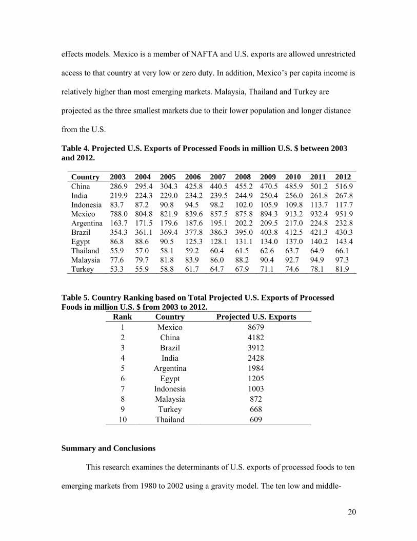
effects models. Mexico is a member of NAFTA and U.S. exports are allowed unrestricted

access to that country at very low or zero duty. In addition, Mexico’s per capita income is

relatively higher than most emerging markets. Malaysia, Thailand and Turkey are

projected as the three smallest markets due to their lower population and longer distance

from the U.S.

Table 4. Projected U.S. Exports of Processed Foods in million U.S. $ between 2003 and 2012.

Country 2003 2004 2005 2006 2007 2008 2009 2010 2011 2012 China 286.9 295.4 304.3 425.8 440.5 455.2 470.5 485.9 501.2 516.9India 219.9 224.3 229.0 234.2 239.5 244.9 250.4 256.0 261.8 267.8Indonesia 83.7 87.2 90.8 94.5 98.2 102.0 105.9 109.8 113.7 117.7Mexico 788.0 804.8 821.9 839.6 857.5 875.8 894.3 913.2 932.4 951.9Argentina 163.7 171.5 179.6 187.6 195.1 202.2 209.5 217.0 224.8 232.8Brazil 354.3 361.1 369.4 377.8 386.3 395.0 403.8 412.5 421.3 430.3Egypt 86.8 88.6 90.5 125.3 128.1 131.1 134.0 137.0 140.2 143.4Thailand 55.9 57.0 58.1 59.2 60.4 61.5 62.6 63.7 64.9 66.1 Malaysia 77.6 79.7 81.8 83.9 86.0 88.2 90.4 92.7 94.9 97.3 Turkey 53.3 55.9 58.8 61.7 64.7 67.9 71.1 74.6 78.1 81.9

Table 5. Country Ranking based on Total Projected U.S. Exports of Processed Foods in million U.S. $ from 2003 to 2012.

Rank Country Projected U.S. Exports 1 Mexico 8679 2 China 4182 3 Brazil 3912 4 India 2428 5 Argentina 1984 6 Egypt 1205 7 Indonesia 1003 8 Malaysia 872 9 Turkey 668 10 Thailand 609

Summary and Conclusions

This research examines the determinants of U.S. exports of processed foods to ten

emerging markets from 1980 to 2002 using a gravity model. The ten low and middle-

20

income countries analyzed included China, India, Indonesia, Brazil, Mexico, Thailand,

Turkey, Egypt, Argentina and Malaysia.

The “modified gravity model” was estimated using two approaches. Empirical

results from the classical linear regression analysis indicate that, consistent with our

hypotheses, population, GDP, level of urbanization and an open trade regime positively

impact U.S. exports of processed foods. As expected, exchange rates and distance were

found to have a negative effect on U.S. exports. These empirical results are consistent

with the findings of Coyle, Gehlhar, Hertel, and Wang (1998) and Regmi, Deepak, Seale,

and Bernstein (2001).

Empirical results from the fixed-effects model are similar to those from the

classical linear regression model, with the exception of population. Population, contrary

to expectations, has a negative relationship with import demand for U.S. processed foods.

However, this negative impact of population is consistent with the findings of Frankel

(1997). Group-effects are present for all the 10 countries and 7 of these are statistically

significant, indicating that the relationship of U.S. exports of processed foods to each of

these 10 countries is unique.

A cross-country comparative analysis was conducted to rank the ten markets for

U.S. exports of processed foods in the future. Countries were ranked on the basis of

predictions for the period 2003-2012 using results from the classical regression model.

Mexico is predicted to be the largest importer of U.S. processed foods, followed by China

and Brazil. So, what do the empirical results of this research imply? Among the emerging

markets, countries with open trade policies offer better opportunities to U.S. exporters of

21

processed foods. Also, middle-income countries that are not too distant from the U.S. are

projected as more lucrative markets.

22

References

Athukorala, P. and K. Sen. “Processed Food Exports from Developing Countries: Patterns and Determinants.” Food Policy 23, 1(1998):41-54. Baier, S.L., and J. H. Bergstrand. “The Growth of World Trade: Tariffs, Transport Costs, and Income Similarity.” Journal of International Economics 53(2001):1–27. Bayoumi, T. and B. Eichengreen. “Is Regionalism Simply a Diversion? Evidence from the EU and EFTA.” In Ito, T. and A. Kreuger (eds.) Regionalism versus Multilateral Trade Arrangements. Chicago: The University of Chicago Press, 1997. Bergstrand, J.H. “The Gravity Equation in International Trade: Some Microeconomic Foundations and Empirical Evidence.” The Review of Economics and Statistics 67, 3(August 1985):474-481. Bougheas, S., P. Demetriades, and E. Morgenroth. “Infrastructure, Transport Costs and Trade.” Journal of International Economics 47(1999):169-189. Burfisher, M. et al. Options for Agricultural Policy Reform in the WTO Negotiations. USDA-ERS, Agricultural Economic Report No. 797, January 2001. Coyle, W.T., M. Gehlhar, T.W. Hertel, Z. Wang and W. Yu. “Understanding the Determinants of structural Change in World Food Markets.” American Journal of Agricultural Economics 80(1998):1052-1062. dell’Aquila, C., R.Sarker and K.Meilke. “Regionalism and Trade in Agrifood Products.” International Agricultural Trade Research Consortium Working Paper 99-5, May 1999. Distances.com. Internet site: www.distances.com Edwards, S. “Openness, Productivity and Growth: What Do We Really Know?” National Bureau of Economic Research Working Paper 5978, March 1997. Feenstra, R.C. “Integration of Trade and Disintegration of Production in the Global Economy.” Journal of Economic Perspectives (Fall 1998):31-50. Fontagné, L., and J.M. Pasteels. “TradeSim (second version).” Market Analysis Section, International Trade Centre, UNCTAD/WTO, May 2003. Frankel, J. “Regional Trading Blocs in the World Economic System.” Washington, D.C.: Institute for International Economics (October 1997):49-76. Frankel, J., E. Stein, S. Wei. “Improving the Design of Regional Trade Agreements, Regional Trading Arrangements: Natural or Supernatural?” The American Economic Review 86, 2(May 1996):52-56.

23

Gehlhar M. and W. Coyle. “Global Food Consumption and Impacts on Trade Pattern.” in Changing Structure of Global Food Consumption and Trade, ed. A. Regmi, pp. 4-13. Washington, D.C: USDA-ERS, WRS-01-1, 2001. Gibson, P., J. Wainio, D. Whitley, and M. Bohman. Profiles of Tariffs in Global Agricultural Markets. Washington, D.C.: USDA – ERS, Market and Trade Economics Division, Agricultural Economic Report No. 796, January 2001. Greene, W.H. Econometric Analysis, 5th ed. Prentice Hall, 2003. Hilsenrath, J.E. “Asian Economic Survey.” The Wall Street Journal, October 23, 2000. Kmenta, J. Elements of Econometrics, 2nd ed. New York: The Macmillan Co., 1986. Kornai, J. The Socialist System: The Political Economy of Communism. Princeton, N.J.: Princeton University Press, 1992. Krugman, P. “Growing World Trade: Causes and Consequences.” Brookings Papers on Economic Activity 1(1995):327-362. Poyhonen, P. “A Tentative Model for the Volume of Trade between Countries.” Weltwertschaftliches Archiv, 90(1963):93-100. Rauch, J.E. “Networks versus Markets in International Trade.” Journal of International Economics 48, 1(1999):7-35. Regmi, A. “Introduction” in Changing Structure of Global Food Consumption and Trade, ed. by A. Regmi. Washington, D.C.: USDA – ERS, Market and Trade Economics Division, Agriculture and Trade Report, WRS-01-1, May 2001. Regmi A. and J. Dyck. “Effects of Urbanization on Global Food Demand” in Changing Structure of Global Food Consumption and Trade, ed. A. Regmi, pp. 23-30. Washington, D.C.: USDA-ERS, Market and Trade Economics Division, Agriculture and Trade Report, WRS-01-1, May 2001. Regmi, A. and M. Gelhar. “Consumer Preferences and Concerns Shape Global Food Trade.” Washington, D.C.: USDA, ERS, Food Review (Sept.-Dec. 2001):2-8 Regmi, A. M.S. Deepak, J.L. Seale Jr. and J.Bernstein. “Cross-Country Analysis of Food Consumption Patterns” in Changing Structure of Global Food Consumption and Trade, ed. A. Regmi, pp. 14-22. Washington, D.C.: USDA-ERS, Market and Trade Economics Division, Agriculture and Trade Report, WRS-01-1, May 2001. Sachs, Jeffrey, A. Warner, A. Aslund and S. Fischer. “Economic Reform and the Process of Global Integration.” Brookings Papers on Economic Activity 1995, 1(1995):1-118.

24

SAS OnlineDoc, version 8. Internet site: http://v8doc.sas.com/sashtml/ (Accessed 2003). STATA. Internet site: www.stata.com/support/faqs/stat/#glm (Accessed 2003). Summary, R.M. “A Political Economic Model of U.S. Bilateral Trade.” The Review of Economics and Statistics 71, 1(February 1989):179-182. Timbergen, J. Shaping the World Economy – Suggestions for an International Economic Policy. New York: Twentieth Century Fund, 1962. U.S. Department of Agriculture, Economic Research Service, Briefing Room. Internet site: www.ers.usda.gov/Briefing/AgTrade/usagriculturaltrade.htm (Accessed April 2003). U.S. Department of Agriculture, Economic Research Service, Foreign Agricultural Trade of the U.S. Internet site: www.ers.usda.gov/data/fatus/DATA/Xcytop15.xls (Accessed April 2004). U.S. Department of Agriculture, Economic Research Service, International Macroeconomic Data Set. Internet site: http://www.ers.usda.gov/Data/macroeconomics/ (Accessed August 2003). U.S. Department of Agriculture, Forces Shaping U.S Agriculture: A Briefing Book. Washington, D.C.: Economic Research Service, July 1997. U.S. Department of Agriculture, Foreign Agricultural Service, U.S. Trade, Exports. Internet site: www.fas.usda.gov/ustrade/USTExFatus (Accessed 2003). United Nations, Population Division, World Urbanization Prospects, The 2001 Revision. Internet site: www.un.org/esa/population/publications/wup2001/wup2001dh.pdf (Accessed October 2003). Wilson, D. and R. Purushothaman. Dreaming with BRICs: The Path to 2050. Goldman Sachs, Global Economics Paper No: 99, October 2003. World Bank, Data and Statistics, Country Classification. Internet site: www.worldbank.org/data/countryclass/countryclass.html (Accessed November 2003).

25

APPENDIX A

Definition of Low and Middle-Income countries:

Income group: Economies are divided according to 2002 GNI per capita, calculated using

the World Bank Atlas method. The groups are: low income, $735 or less; lower middle

income, $736 - $2,935; upper middle income, $2,936 - $9,075; and high income, $9,076

or more (The World Bank, 2004)

China Lower-middle-income India Low-income Indonesia Low-income Thailand Lower-middle-income Malaysia Upper-middle-income Egypt Lower-middle-income Turkey Lower-middle-income Brazil Lower-middle-income Argentina Upper-middle-income Mexico Upper-middle-income

26