energies

Article

Demand Response Resource Allocation MethodUsing Mean-Variance Portfolio Theory for LoadAggregators in the Korean Demand Response Market

Jaeyong Chae and Sung-Kwan Joo *

School of Electrical Engineering, Korea University, Seoul 02841, Korea; chaejae@korea.ac.kr* Correspondance: skjoo@korea.ac.kr; Tel.: +82-2-3290-3927

Received: 2 May 2017; Accepted: 24 June 2017; Published: 29 June 2017

Abstract: Since the demand response (DR) market was introduced in Korea, load aggregators havealso been allowed to participate in the electricity market. However, a risk-management-based methodfor the efficient operation of demand response resources (DRRs) has not been studied from the loadaggregators’ perspective. In this paper, a systematic DRR allocation method is proposed for loadaggregators to operate DRRs using mean-variance portfolio theory. The proposed method is designedto determine the lowest-risk DRR portfolio for a given level of expected return using mean-varianceportfolio theory from the perspective of load aggregators. The numerical results show that theproposed method can be used to reduce the risk compared to that obtained by the baseline method,in which all individual DRRs are allocated in a DRR group by maximum curtailment capability.

Keywords: demand response resource; mean-variance portfolio theory; expected return and risk;load aggregators

1. Introduction

The demand response (DR) market was introduced in the Korean electricity market in November2014. In the past, demand management was implemented through the program by Korea ElectricPower Corporation (KEPCO) in Korea. However, after the DR market was opened, a third party called“the load aggregator” was allowed to participate in the Korean electricity market. Load aggregatorshave recruited the resources of KEPCO’s customers who have participated in demand management.Thus, there has not been any difficulty in recruiting demand response resources (DRRs). However,due to the lack of business experiences of the load aggregators, there was not enough priorknowledge on the efficient operation and management of aggregated DRRs. The profitability ofaggregators varies depending upon how the aggregators manage the DRRs because various DRRshave different characteristics.

In this study, a mean-variance portfolio method is proposed for determining the lowest-riskDRR portfolio for a given level of expected return for load aggregators. The proposed method isdesigned to compute the expected return and risk of a DRR portfolio by considering DRRs’ variouscharacteristics such as the maximum curtailment capability, sustained response duration, and historicalparticipation rate.

Markowitz’s mean-variance portfolio theory [1] suggests how to minimize the risk of a portfoliobased on the expected returns and risks of individual assets. The correlation among the expectedreturns of individual assets can reduce risk when assembling a portfolio of assets. This is named theportfolio effect or diversification effect. Portfolio theory was applied initially in the financial field andhas subsequently been applied in the field of energy research. Bar-Lev and Katz, in early examples ofapplying portfolio theory to the electric power field, proposed a method to optimize the fossil fuelgeneration mix and determined the extent to which the electricity industry has utilized fossil fuel

Energies 2017, 10, 879; doi:10.3390/en10070879 www.mdpi.com/journal/energies

Energies 2017, 10, 879 2 of 14

resources in [2]. Awerbuch and Berger evaluated the application of portfolio theory to the developmentof an optimal generation mix in the European Union (EU), and illustrated the portfolio effects, i.e.,diversification effects of different generating mixes in [3]. In [4], Jansen et al. presented the resultsof an application of portfolio theory to a future portfolio of electricity generating technologies in theNetherlands by 2030, and they identified that portfolio (cost) risk can be reduced significantly throughdiversification with a critical role for renewable generation such as wind power. In [5], Delarue etal. applied portfolio theory to establish a multi-period power generation mix plan, and illustratedthat the introduction of wind power can be motivated by a desire to lower the risk on generation cost.In [6], Eichhorn and Römisch presented a model for finding an electricity portfolio that maximizesprofits and minimizes risk when retailers procure the power they need to supply using polyhedralrisk measures.

There have been various studies related to optimizing the operation of DRRs. In reference [7],DRRs can be considered as a means to avoid the risk by the fluctuation of electricity prices and demandfrom the perspective of load-serving entities (LSEs). On the other hand, the proposed method in thispaper attempts to determine the lowest risk DRR portfolio for a given level of expected return usingmean-variance portfolio theory from the load aggregators’ perspective. In [8], Mollahassani-pour et al.proposed a method to minimize the cost while maintaining the reliability of a system by consideringthe DRRs in establishing the preventive maintenance plan of the generator, assuming the DRR asthe virtual power plant. In [9], Dabbagh and Sheikh-El-Eslami proposed an offering model for avirtual power plant, which is an integration of various distributed energy resources, using a two-stagestochastic programming approach and conditional value at risk (CVR).

The market-bidding problem of a pool of price-responsive consumers for the aggregator or theretailer is studied in [10]. The complex market bid, consisting of a series of price-energy bidding curves,consumption limits, and maximum pike-up and drop-off rates, can largely capture the price-sensitiveconsumption of the cluster of flexible loads. In [11], the relation between electricity price and customerresponse is analyzed by applying stochastic finite impulse response (FIR) model. A bidding approachfor a time-shiftable load in the day-ahead and real-time markets is proposed in [12] to minimize energyprocurement cost. The bidding strategy of plug-in electric vehicle aggregator proposed in [13]. Biddingand clearing strategy is developed in [14] by incorporating the internal dynamics of thermostaticallycontrolled loads into mechanism design problem. These studies deal with the price-bid strategy ofthe aggregator or the retailer in various electricity market, but the return and risk faced by them isnot considered.

Portfolio theory has been applied in the field of power research primarily for the optimizationof the generation mix and procurement of electricity. In addition, studies on DRRs have thus farfocused on effective operation of the resources. However, there has not been any research conductedto measure the profitability and risk of the resources and allocate them by applying portfolio theory.

The present work outlines an approach to assess the rate of return and the risk of DRRs and tooptimize the operation of many DRRs using Markowitz portfolio theory. Section 2 provides details ofthe calculation method for the expected return and risk of an individual DRR (each customer). Section 3details the method of grouping resources using portfolio theory. Section 4 reports on numerical results,and Section 5 discusses the conclusion and paths forward.

2. How to Measure Expected Returns and Risks of Individual Resources

2.1. Background

Markowitz’s portfolio theory, or mean-variance analysis, is a mathematical framework to assemblea portfolio of assets such that the risk is minimized for a given level of expected return, and the expectedreturn and risk of an asset are defined to be the mean and variance (or standard deviation) of anasset’s rate of return, respectively. This theory was originally developed in the finance field, but ifthe expected return and risk of an asset can be measured in a reasonable way, it can be applied in

Energies 2017, 10, 879 3 of 14

various fields such as a generation mix and DRRs operation. In particular, because load aggregatorsmust operate so many DRRs, it is very useful to apply portfolio theory in grouping the resources andoperating them to minimize the risk or maximize the profit.

Load aggregators hold many DRRs (end use customers) that have quite different characteristicssuch as reduction capacity, ramp period (or response time), and sustained response period. Theseresources would respond differently according to their business environment, and rewards for loadreduction and penalties for reduction failure are offered by the market price, so the characteristics ofeach resource (customer) and the market price have an effect on the revenues of load aggregators.

2.2. Market Price and Participation Rate

Since electricity market prices are used to determine both compensation for curtailment andpenalties by failure to curtail, the market price is a significant factor to influence the profit of loadaggregators. Market prices are determined by the principle of supply and demand in the electricitymarket and generally changes according to various market conditions such as loads, fuel prices, andgenerator maintenance schedule. Because electricity market prices are dynamic, they can be generallymodeled using the geometric Brownian motion (GBM) model [15–17]. Thus, prices in the future in thisstudy are estimated by the following GBM model:

dP = µpP dt + σpP dz (1)

where P and µp represent electricity market price and a drift rate of electricity market price, respectively.σp, dt, and dz denote volatility of electricity market price, time interval and generalized Wiener process,respectively. µp and σp are estimated from Korea’s electricity market price data during years 2014–2016.

Customers, i.e., individual DRRs, may fail to achieve the contracted curtailment capabilityallocated by an aggregator. In a case where the customer fails to curtail, the market operator imposesthe penalty on the aggregator due to the curtailment failure. In the other words, the uncertainty in thebehavior of customers’ response influences aggregators’ profit, and the participation rate is a criticalfactor in the revenue stream of load aggregators.

The behaviors relating to participation can be analyzed by using historical load curtailment data.If DRRs do not participate when curtailment is instructed, there will be a higher probability thatDRRs will not participate in the very near future as well. In this study, the future participation rateis estimated using the past participation rate and GBM model. The past participation rate (πpast

i ) iscalculated from the data of historical load curtailment in Korea Electric Power Corporation (KEPCO)DR program as follows:

πpasti =

DRpastit, prov

DRpastit

(2)

where DRpastit is the DRR requested by the load aggregator to customer i at time t in the past demand

response event, and DRpastit,prov is the amount of the load curtailment provided by customer i at time t in

the past DR event.In practice, various factors such as temperature, humidity, electricity prices and operating

schedules in factories can affect customer’s electricity consumption. These factors also influenceparticipants in demand response in a similar manner, but differently depending upon whether theparticipants are residential or industrial. Consumption patterns of residential participants couldpossibly be more weather dependent, whereas those of industrial participants could be more operatingschedule dependent. However, regardless of consumer types, the primary driver to manage theconsumption patterns of any electricity consumer and draw the participations in demand response isthe price signal. The price signal in the market is the key factor affecting the decision-making on thedemand side as to whether to participate or not. The participation in demand response is generallydependent upon the degree of the compensation and status of the price signal. For example, owners of

Energies 2017, 10, 879 4 of 14

DRRs with lower shutdown cost would participate in demand response even when electricity priceis relatively low. On the other hand, owners of DRRs with higher shutdown cost would preferablyparticipate in demand response whenever the price is relatively high enough to recover its shutdowncost. Despite the fact that there have been former studies dealing with consumers’ responses toelectricity prices [10], the participation rate is considered in this study to be a dependent variable of theelectricity price and participation rate in the future is estimated through regression model as follows:

PRit = ai Pt + bi (3)

where PRit represents the participation rate of DRR i at time t.The first-order coefficient, ai, and the constant term, bi, are estimated by linear regression model

using the past participation rate (πpastit ) and electricity price data. The electricity price at time t, i.e.,

Pt, which is used in the future participation rate estimation, is based on the price data estimated bythe GBM model. Because Pt is a dynamic variable estimated using stochastic process model, PRit isalso dynamic.

2.3. Revenue and Cost of Load Reduction

2.3.1. Overview of Demand Response Market in Korea

Demand response resources have been traded in the Korean wholesale electricity market sinceNovember 2014. In the DRR market, peak curtailment DRRs (or capacity DRRs) and price responsiveDRRs are traded separately. In the case of peak curtailment DRRs, Korea Power Exchange (KPX)(Independent System Operator in Korea Electricity Market) instructs a load curtailment an hourahead, and these resources assume a role to substitute for high-cost generators. The customersparticipating in the load curtailment are compensated with incentives such as payments for availabilityand performance. The payment for availability is calculated in the same method as the capacity price ofgenerators and the payment for performance is determined based on the resources’ actual curtailmentand the highest variable generation cost at that time. In the case of price responsive DRR, the resourcesbid on the day-ahead electricity market and curtail the load if the demand reduction price is lowerthan the bid prices of generators, and are compensed with incentives based on the system marginalprice (SMP).

2.3.2. Revenue from Load Curtailment

Regarding load aggregators, revenue from the load curtailment of a customer (or individual DRR)includes market payment and customer penalties. Market payment includes payment for scheduledcurtailment, payment for dispatched curtailment, and payment for capability. Payment for scheduledcurtailment is a reward for the amount of load curtailment assigned in a day-ahead unit commitment(UC), and is determined based on system marginal price (SMP) in the electricity market. Payment fordispatched curtailment is a reward for the amount of the load curtailment assigned in an-hour-aheaddispatch and determined based on the highest variable cost of all operating generators. Paymentfor capacity is a reward for the obligatory curtailment capacity. Customer penalties are payment forfailing to curtail the scheduled load and are determined by a contract between a load aggregator anda customer.

Revenue = Market payment + Customer penalty (4)

Market payment= Payment for scheduled curtailment+Payment for dispatched curtailment+Payment for availability (capability)

(5)

Energies 2017, 10, 879 5 of 14

2.3.3. Cost of Load Curtailment

The costs of a load aggregator for load curtailment consist of customer incentives and marketpenalties. Customer incentives are payments paid to a customer to participate in load curtailment andare determined by a contract between a load aggregator and a customer such as customer penalties.Market penalties are payments for failing to reduce. If a load aggregator did not carry out the loadcurtailment assigned in a day-ahead UC, KPX imposes penalties for scheduled curtailment on theaggregator. In addition, if a load aggregator fails to carry out the load curtailment dispatched, KPXimposes penalties for dispatched curtailment on the aggregator. Penalties for scheduled curtailmentare determined based on SMP, and penalties for dispatched curtailment are determined as the cutbackof the payment for capacity.

Cost = Customer incentive + Market penalty (6)

Market penalty = Penalty for scheduled curtailment+Penalty for dispatched curtailment

(7)

2.3.4. Rate of Return of an Aggregator by the Load Curtailment of Each Customer

A rate of return (RORi ) that a load aggregator can obtain when a customer (individual DRR i) ofthe aggregator participates in load curtailment is defined as follows:

RORi =REVMP

i(

DRsi)+ REVPE

i(

DRsi)− COST INCT

i(

DRsi)− COSTPE

i(

DRsi)

COST INCTi

(DRs

i)+ COSTPE

i(

DRsi) (8)

where DRsi is the amount of load reduction that customer i contributes for scenario s as follows:

DRsi = DRalloc

i ·πsi , ∀ i, s (9)

REVMPi is the revenue obtained in payment for the load curtailment by customer i. It increases

proportionally with increasing actual amount of load curtailment by customer i when the customer’sactual load curtailment is less than or equal to 120% of the load reduction assigned to customer i in theDR event. However, if the actual amount of the customer’s load curtailment is greater than 120% of theamount of load curtailment allocated by the aggregator, no further revenue resulting from receivingDR market prices is generated. The function REVMP

i is defined as follows:

REVMPi (DRs

i ) = MPs·min(

DRsi , DRalloc

i × 1.2)

, ∀ i, s (10)

where MPs is the wholesale electricity market price for scenario s, DRsi is the actual load curtailment

of customer i for scenario s, and DRalloci is the amount of load curtailment allocated to customer i.

REVPEi is the revenue obtained only when customer i does not curtail some or all of the allocated

load curtailment in the DR event. The penalty imposed on customer i by the aggregator is the penaltyprice (PEi ) multiplied by the difference between the actual and allocated amount of load curtailmenton customer i. This function is expressed as follows:

REVPEi (DRs

i ) = PEi·max(

DRalloci − DRs

i , 0)

, ∀ i, s (11)

where PEi is price of the penalty determined by a contract between an aggregator and customer i.COST INCT

i is an incentive offered as the reward for load reduction to customer i that participatesin the DR event by the aggregator. It increases proportionally with increasing actual amount of loadreduction by customer i when the customer’s actual load reduction is less than or equal to the loadcurtailment assigned to customer i in the DR event. However, if the actual amount of the customer’s

Energies 2017, 10, 879 6 of 14

load reduction is greater than the customer’s load curtailment assigned by the aggregator, there is nofurther cost to pay for additional load reduction. The function COST INCT

i is defined as follows:

COST INCTi (DRs

i ) = INCTi·min(

DRsi , DRalloc

i

), ∀ i, s (12)

where INCTi is the incentive price determined by a contract between an aggregator and customer i.COSTPE

i is an expense that should be paid to the ISO by the aggregator who fails to meet theamount of curtailment allocated by the ISO (KPX) because customer i does not reduce some or all ofallocated load curtailment in the DR event. If a customer does not curtail as much as allocated byits aggregator, the deficit is covered by another customer of the aggregator and the aggregator is notcharged a penalty. However, because the aggregator should pay the price to the customer covering thedeficit, the cost increases. Thus, COSTPE

i is the price for load reduction of the customer covering thedeficit, however, the unit price is equal to the price for the load curtailment of customer i. This functionis expressed as follows:

COSTPEi (DRs

i ) = INCTi·min(

DRalloci − DRs

i , 0)

, ∀ i, s (13)

2.4. Calculation of Expected Returns and Risks

In this study, a Monte Carlo simulation-based method is used to calculate the expected return,risk, and covariance, i.e., correlation coefficient of DRRs. In this paper, the primary factors affectingthe rate of returns of aggregators are assumed to be the participation rate and wholesale electricitymarket price. Therefore, future price and participation rate need to be estimated in order to calculatethe rate of return for an individual DRR. The stochastic model described in Section 2.2 is applied toestimate the future price and participation rate. The amount of curtailment from DRR, revenue, cost,and rate of return are computed using the estimated future prices and participation rates. The mean,i.e., expected return and the variance, i.e., risk of a portfolio are computed by Monte Carlo simulations

3. Resource Allocation Method Using Portfolio Theory

In this section, a new method is proposed for optimally grouping DRRs, the load curtailment ofall customers contracting with a load aggregator to reduce their loads, using the expected return andrisk of the individual DRR by applying portfolio theory.

3.1. Resource Grouping Scenario

ere are many ways by which a load aggregator divides its customers (individual resources) intoDRR groups. For example, dividing 10 individual resources into two DRR groups results in a numberof 1024 (=210), and with increasing number of individual resources and DRR groups, the number ofpossible divisions increases very quickly. However, not all cases are considered because there aresome constraints related to formulating DRRs. In the Korean DR market, one DRR group shall becomposed of 10 or more individual DRRs, and the maximum reduction capacity of one DRR groupshall be 10–500 MW. Therefore, in this study, the cases that satisfy these constraints are considered anddefined a dividing case as a “scenario”. Figure 1 roughly shows how an aggregator can divide all itsindividual DRRs into some (N) DRR groups.

Each individual resource has its own load characteristics. Some resources have a high load factor,some have a low load factor, and the shape of the load duration curve (LDC) varies from resource toresource. One DRR group can minimize the risk from the aggregator’s point of view by complementingthem if resources with different load characteristics are evenly included. Therefore, the DRR group isconstructed by reflecting the load characteristics of the individual resources.

A DRR group is simply a collection of DRRs aggregated by a load aggregator. The load aggregatorcan operate multiple DRR groups. A scenario is one of all possible DRR combinations by combiningdifferent DRRs to form a DRR group. A portfolio is constructed by taking a weighted combination of

Energies 2017, 10, 879 7 of 14

DRRs with different composition ratios, i.e., weights of DRRs on their curtailment capabilities in a DRRgroup. Therefore, it is possible to create various types of portfolios by taking different compositionratios of DRRs in the same DRR group.

Energies 2017, 10, 879 6 of 13

the deficit, however, the unit price is equal to the price for the load curtailment of customer i. This function is expressed as follows: ( ) = ∙ min( − , 0), ∀ , (13)

2.4. Calculation of Expected Returns and Risks

In this study, a Monte Carlo simulation-based method is used to calculate the expected return, risk, and covariance, i.e., correlation coefficient of DRRs. In this paper, the primary factors affecting the rate of returns of aggregators are assumed to be the participation rate and wholesale electricity market price. Therefore, future price and participation rate need to be estimated in order to calculate the rate of return for an individual DRR. The stochastic model described in Section 2.2 is applied to estimate the future price and participation rate. The amount of curtailment from DRR, revenue, cost, and rate of return are computed using the estimated future prices and participation rates. The mean, i.e., expected return and the variance, i.e., risk of a portfolio are computed by Monte Carlo simulations

3. Resource Allocation Method Using Portfolio Theory

In this section, a new method is proposed for optimally grouping DRRs, the load curtailment of all customers contracting with a load aggregator to reduce their loads, using the expected return and risk of the individual DRR by applying portfolio theory.

3.1. Resource Grouping Scenario

There are many ways by which a load aggregator divides its customers (individual resources) into DRR groups. For example, dividing 10 individual resources into two DRR groups results in a number of 1024 (=2 ), and with increasing number of individual resources and DRR groups, the number of possible divisions increases very quickly. However, not all cases are considered because there are some constraints related to formulating DRRs. In the Korean DR market, one DRR group shall be composed of 10 or more individual DRRs, and the maximum reduction capacity of one DRR group shall be 10–500 MW. Therefore, in this study, the cases that satisfy these constraints are considered and defined a dividing case as a “scenario”. Figure 1 roughly shows how an aggregator can divide all its individual DRRs into some (N) DRR groups.

Figure 1. Schemes of dividing individual demand response resources (DRRs) into DRR groups.

Each individual resource has its own load characteristics. Some resources have a high load factor, some have a low load factor, and the shape of the load duration curve (LDC) varies from resource to

Figure 1. Schemes of dividing individual demand response resources (DRRs) into DRR groups.

3.2. Minimum Variance Portfolio Selection of Optimal Grouping Scenario

There are several DRR groups in a scenario and, for each group, we can construct many portfolioswith individual DRRs included in each DR resource. Then the expected return and risk of the portfoliosare calculated. The expected return and risk of a portfolio are defined as follows:

E(RP) =n

∑i=1

wi·E(Ri) (14)

σ2P =

n

∑i=1

wi·wj·σij (15)

where wi is a share of individual DRR i in the portfolio, E(Ri) is an expected return of individual DRRi, σ2

P is a variance of an individual DRR’s return, and σij is a covariance between the rate of returns ofindividual DRRs i and j.

Once the expected return and risk of portfolios are calculated, the minimum variance portfolio(MVP) for each DRR group can be determined. The MVP is the portfolio whose risk (variance orstandard deviation) is the least among all portfolios that can be created with individual DRRs includedin a DRR group. A “group risk” (RISKgrp

i ) can be defined to be the risk of the MVP and define a“scenario risk” (RISKscn

s ), as the mean of all group risks of that scenario. The final objective is todetermine the optimal scenario, which has the lowest scenario risk, and which is the best way to groupindividual DRRs. Combining the above steps, the following optimization problem can be formulatedas follows:

min{s}

RISKscns =

1N

N

∑i=1

RISKgrpi (16)

RISKgrpi = min

{wi ,wj}σ2

P =n

∑i=1

n

∑j=1

wi·wj·σij (17)

Energies 2017, 10, 879 8 of 14

n

∑i=1

wi = 1 (18)

n

∑j=1

xij ≥ Ngrp (19)

dmin ≤N

∑j=1

xij·dj ≤ dmax (20)

Emin ≤N

∑j=1

xij·dj·τj ≤ Emax (21)

where xij is a binary variable indicating whether individual DRR j is included in DRR group i (i.e.,if included, 1; otherwise, 0). Ngrp is the minimum number of individual DRRs to be included inone DRR group, dj is the maximum amount of load curtailment capacity for individual DRR j, anddmin and dmax are the minimum and maximum amounts of total load capacity (MW), respectively, thatone DRR group should reduce in a DR event. τj is the maximum curtailment duration of individualDRR j, and Emin and Emax are the minimum and maximum amounts of total energy (MWh), respectively,that one DRR group should curtail in a DR event.

3.3. Target Return and Risk

MVP has the advantage of minimizing risk, but it has the weakness that the expected return isalso lowered. For this reason, aggregators are inevitably interested in how to construct a resource thatcan achieve a reasonable expected return. This can be overcome by slightly modifying the methodpresented above. By adding the target expected rate of return and the target risk as constraints whilekeeping the objective function that minimizes the risk, it is possible to achieve two goals: securing theappropriate rate of return and minimizing the risk. The following constraint expression is added:

n

∑i=1

wi·E(Ri) = E(Rp)target (22)

n

∑i=1

wi·wj·σij = σ2p

target(23)

4. Numerical Results

Figure 2 shows the overall algorithm of the proposed method described in the previous chapter.In this section, according to this algorithm, the proposed DRR allocation method is numerically testedusing historical data of customers (individual DRRs) who have participated in KEPCO’s DR program.There have been few attempts to study how the recruited demand response resources can be managedeffectively with respect to rate of return and risk from a research perspective. Furthermore, sincethe aggregator does not disclose how they actually manage resources, it is difficult to recognize howexactly and what method is being used in practice. Therefore, the performance of the proposed methodis compared with the baseline method. The baseline method is designed to determine a compositionratio of individual demand response resources in a portfolio based on their reduction capabilities.

4.1. Assumptions and Data

In the numerical test, to simplify the discussion, a load aggregator was assumed to attemptto constitute two DRR portfolios from 14 individual resources and participates in the onlyprice-responsive DR market. To optimize the resource constitution, the load aggregators considerthe maximum curtailment capability (or capacity), load factors and participation rates of individualcustomers. The participation rate (πi) is calculated using historical load curtailment data of individual

Energies 2017, 10, 879 9 of 14

resources in the DR program conducted by KEPCO, and load factors are derived from load data byindustry. Wholesale electricity market prices (MPs) and penalty prices for individual resources (PEi)are estimated using historical SMP data from the Korea Electricity Exchange (KPX). It is assumed thatthe unit price of customer incentives for individual resources (INCTi) are calculated considering theretail price. The characteristics of individual resources are presented in Table 1.

Energies 2017, 10, 879 8 of 13

one DRR group, is the maximum amount of load curtailment capacity for individual DRR j, and are the minimum and maximum amounts of total load capacity (MW), respectively, that one DRR group should reduce in a DR event. is the maximum curtailment duration of individual DRR j, and and are the minimum and maximum amounts of total energy (MWh), respectively, that one DRR group should curtail in a DR event.

3.3. Target Return and Risk

MVP has the advantage of minimizing risk, but it has the weakness that the expected return is also lowered. For this reason, aggregators are inevitably interested in how to construct a resource that can achieve a reasonable expected return. This can be overcome by slightly modifying the method presented above. By adding the target expected rate of return and the target risk as constraints while keeping the objective function that minimizes the risk, it is possible to achieve two goals: securing the appropriate rate of return and minimizing the risk. The following constraint expression is added:

∙ ( ) = ( ) (22)

∙ ∙ = (23)

Figure 2. Algorithm of proposed method.

4. Numerical Results

Figure 2 shows the overall algorithm of the proposed method described in the previous chapter. In this section, according to this algorithm, the proposed DRR allocation method is numerically tested using historical data of customers (individual DRRs) who have participated in KEPCO’s DR program. There have been few attempts to study how the recruited demand response resources can be managed effectively with respect to rate of return and risk from a research perspective. Furthermore, since the aggregator does not disclose how they actually manage resources, it is difficult to recognize how exactly and what method is being used in practice. Therefore, the performance of the proposed method is compared with the baseline method. The baseline method is designed to determine a

Figure 2. Algorithm of proposed method.

Table 1. The characteristics of individual resources.

Number Name Capacity(MW)

Load Factor(%) Number Name Capacity

(MW)Load Factor

(%)

1 Iron 225 81 8 Paper 3 852 Steel 111.4 81 9 Railway 0.2 623 Cement 1 23 72 10 Electronic 3 854 Cement 2 50 72 11 Waste 0.8 815 Machinery 30 46 12 Wholesale 1 0.6 496 Chemicals 1 23 86 13 Wholesale 2 0.67 497 Chemicals 2 150 86 14 Accommodation 0.62 65

4.2. Expected Returns and Risks of Individual Resources

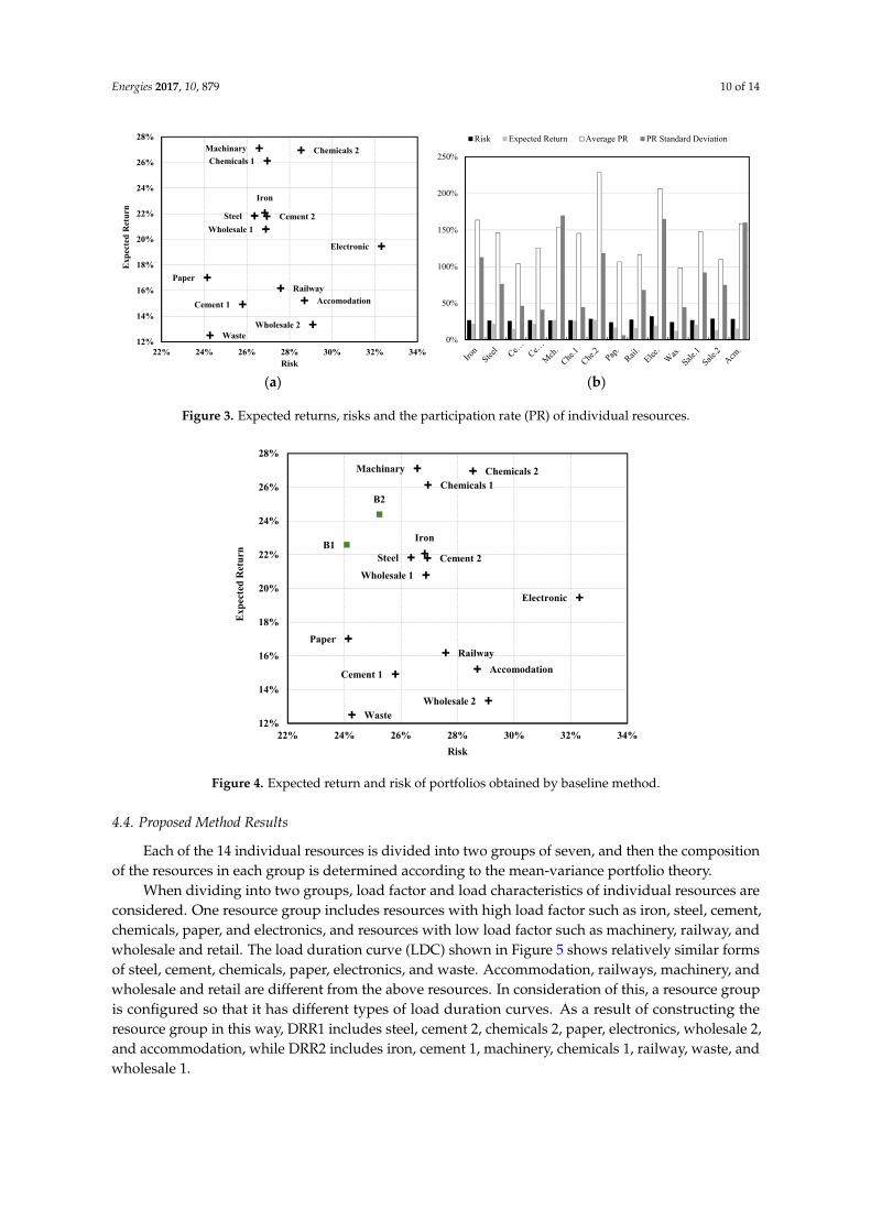
Large-capacity resources such as iron, steel, cement, machinery, and chemicals are more profitableand less risky than small-capacity resources such as railways, wholesale and retail, and accommodation,as shown in Figure 3a. Resources with large variation in participation rate (electronic, accommodation,chemicals 2) showed relatively high risk as shown in Figure 3b.

4.3. Baseline Method

The composition ratio of individual resources is determined based on the reduction capacity ofeach resource, and the expected return and risk are not considered. The expected returns of configuredDRR portfolios (B1 and B2) are 22.6% and 24.4%, and the risks of B1 and B2 are 24.1% and 25.2%,respectively. As shown in Figure 4, configured DRR portfolios (B1 and B2) have a much lower riskthan individual resources because of the risk diversification effect of the portfolio.

Energies 2017, 10, 879 10 of 14

Energies 2017, 10, 879 9 of 13

composition ratio of individual demand response resources in a portfolio based on their reduction capabilities.

4.1. Assumptions and Data

In the numerical test, to simplify the discussion, a load aggregator was assumed to attempt to constitute two DRR portfolios from 14 individual resources and participates in the only price-responsive DR market. To optimize the resource constitution, the load aggregators consider the maximum curtailment capability (or capacity), load factors and participation rates of individual customers. The participation rate ( ) is calculated using historical load curtailment data of individual resources in the DR program conducted by KEPCO, and load factors are derived from load data by industry. Wholesale electricity market prices ( ) and penalty prices for individual resources ( ) are estimated using historical SMP data from the Korea Electricity Exchange (KPX). It is assumed that the unit price of customer incentives for individual resources ( ) are calculated considering the retail price. The characteristics of individual resources are presented in Table 1.

Table 1. The characteristics of individual resources.

Number Name Capacity (MW)

Load Factor(%)

Number Name Capacity (MW)

Load Factor(%)

1 Iron 225 81 8 Paper 3 85 2 Steel 111.4 81 9 Railway 0.2 62 3 Cement 1 23 72 10 Electronic 3 85 4 Cement 2 50 72 11 Waste 0.8 81 5 Machinery 30 46 12 Wholesale 1 0.6 49 6 Chemicals 1 23 86 13 Wholesale 2 0.67 49 7 Chemicals 2 150 86 14 Accommodation 0.62 65

4.2. Expected Returns and Risks of Individual Resources

Large-capacity resources such as iron, steel, cement, machinery, and chemicals are more profitable and less risky than small-capacity resources such as railways, wholesale and retail, and accommodation, as shown in Figure 3a. Resources with large variation in participation rate (electronic, accommodation, chemicals 2) showed relatively high risk as shown in Figure 3b.

(a) (b)

Figure 3. Expected returns, risks and the participation rate (PR) of individual resources.

4.3. Baseline Method

The composition ratio of individual resources is determined based on the reduction capacity of each resource, and the expected return and risk are not considered. The expected returns of configured DRR portfolios (B1 and B2) are 22.6% and 24.4%, and the risks of B1 and B2 are 24.1% and

Iron

Steel

Cement 1

Cement 2

MachinaryChemicals 1

Chemicals 2

PaperRailway

Electronic

Waste

Wholesale 1

Wholesale 2

Accomodation

12%

14%

16%

18%

20%

22%

24%

26%

28%

22% 24% 26% 28% 30% 32% 34%

Exp

ecte

d R

etur

n

Risk

0%

50%

100%

150%

200%

250%

Risk Expected Return Average PR PR Standard Deviation

Figure 3. Expected returns, risks and the participation rate (PR) of individual resources.

Energies 2017, 10, 879 10 of 13

25.2%, respectively. As shown in Figure 4, configured DRR portfolios (B1 and B2) have a much lower risk than individual resources because of the risk diversification effect of the portfolio.

Figure 4. Expected return and risk of portfolios obtained by baseline method.

4.4. Proposed Method Results

Each of the 14 individual resources is divided into two groups of seven, and then the composition of the resources in each group is determined according to the mean-variance portfolio theory.

When dividing into two groups, load factor and load characteristics of individual resources are considered. One resource group includes resources with high load factor such as iron, steel, cement, chemicals, paper, and electronics, and resources with low load factor such as machinery, railway, and wholesale and retail. The load duration curve (LDC) shown in Figure 5 shows relatively similar forms of steel, cement, chemicals, paper, electronics, and waste. Accommodation, railways, machinery, and wholesale and retail are different from the above resources. In consideration of this, a resource group is configured so that it has different types of load duration curves. As a result of constructing the resource group in this way, DRR1 includes steel, cement 2, chemicals 2, paper, electronics, wholesale 2, and accommodation, while DRR2 includes iron, cement 1, machinery, chemicals 1, railway, waste, and wholesale 1.

Figure 5. Load duration curves (LDCs) of individual resources.

Iron

Steel

Cement 1

Cement 2

MachinaryChemicals 1

Chemicals 2

PaperRailway

Electronic

Waste

Wholesale 1

Wholesale 2

Accomodation

B1

B2

12%

14%

16%

18%

20%

22%

24%

26%

28%

22% 24% 26% 28% 30% 32% 34%

Exp

ecte

d R

etur

n

Risk

0%

20%

40%

60%

80%

100%

1 1001 2001 3001 4001 5001 6001 7001 8001

Load

Fac

tor

HourSteel Cement MachineryChemicals Paper RailwayElectronic Waste WholesaleAccomodation

Figure 4. Expected return and risk of portfolios obtained by baseline method.

4.4. Proposed Method Results

Each of the 14 individual resources is divided into two groups of seven, and then the compositionof the resources in each group is determined according to the mean-variance portfolio theory.

When dividing into two groups, load factor and load characteristics of individual resources areconsidered. One resource group includes resources with high load factor such as iron, steel, cement,chemicals, paper, and electronics, and resources with low load factor such as machinery, railway, andwholesale and retail. The load duration curve (LDC) shown in Figure 5 shows relatively similar formsof steel, cement, chemicals, paper, electronics, and waste. Accommodation, railways, machinery, andwholesale and retail are different from the above resources. In consideration of this, a resource groupis configured so that it has different types of load duration curves. As a result of constructing theresource group in this way, DRR1 includes steel, cement 2, chemicals 2, paper, electronics, wholesale 2,and accommodation, while DRR2 includes iron, cement 1, machinery, chemicals 1, railway, waste, andwholesale 1.

Energies 2017, 10, 879 11 of 14

Energies 2017, 10, 879 10 of 13

25.2%, respectively. As shown in Figure 4, configured DRR portfolios (B1 and B2) have a much lower risk than individual resources because of the risk diversification effect of the portfolio.

Figure 4. Expected return and risk of portfolios obtained by baseline method.

4.4. Proposed Method Results

Each of the 14 individual resources is divided into two groups of seven, and then the composition of the resources in each group is determined according to the mean-variance portfolio theory.

When dividing into two groups, load factor and load characteristics of individual resources are considered. One resource group includes resources with high load factor such as iron, steel, cement, chemicals, paper, and electronics, and resources with low load factor such as machinery, railway, and wholesale and retail. The load duration curve (LDC) shown in Figure 5 shows relatively similar forms of steel, cement, chemicals, paper, electronics, and waste. Accommodation, railways, machinery, and wholesale and retail are different from the above resources. In consideration of this, a resource group is configured so that it has different types of load duration curves. As a result of constructing the resource group in this way, DRR1 includes steel, cement 2, chemicals 2, paper, electronics, wholesale 2, and accommodation, while DRR2 includes iron, cement 1, machinery, chemicals 1, railway, waste, and wholesale 1.

Figure 5. Load duration curves (LDCs) of individual resources.

Iron

Steel

Cement 1

Cement 2

MachinaryChemicals 1

Chemicals 2

PaperRailway

Electronic

Waste

Wholesale 1

Wholesale 2

Accomodation

B1

B2

12%

14%

16%

18%

20%

22%

24%

26%

28%

22% 24% 26% 28% 30% 32% 34%

Exp

ecte

d R

etur

n

Risk

0%

20%

40%

60%

80%

100%

1 1001 2001 3001 4001 5001 6001 7001 8001

Load

Fac

tor

HourSteel Cement MachineryChemicals Paper RailwayElectronic Waste WholesaleAccomodation

Figure 5. Load duration curves (LDCs) of individual resources.

The portfolio that minimizes the risk with the same rate of return for each of portfolios (B1 andB2) obtained by the baseline method is A1 and A2 for each group, respectively, and the portfolios thatmaximize returns with the same risk are C1 and C2, respectively. The expected returns and risks forthe portfolios constructed according to the proposed method are shown in Figure 6.

Energies 2017, 10, 879 11 of 13

The portfolio that minimizes the risk with the same rate of return for each of portfolios (B1 and B2) obtained by the baseline method is A1 and A2 for each group, respectively, and the portfolios that maximize returns with the same risk are C1 and C2, respectively. The expected returns and risks for the portfolios constructed according to the proposed method are shown in Figure 6.

The risks for portfolios A1 and A2 were 21.9% and 23.9%, respectively, down 9.1% and 5.2% from the risk for portfolio (B1 and B2) obtained by the baseline method. Expected returns of portfolios C1 and C2 were 24.5% and 25.9%, respectively, which were 8.4% and 6.1%, higher than the expected returns of portfolio (B1 and B2) obtained by the baseline method. In other words, constructing the portfolio by the proposed method can reduce the risk or increase the profit rate.

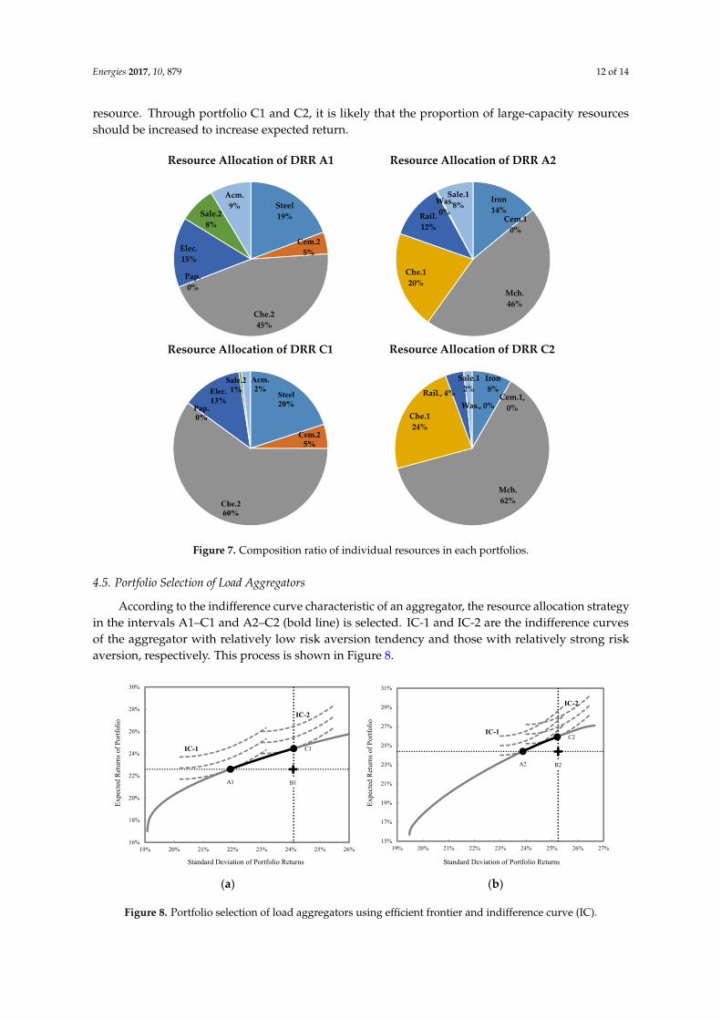
Figure 6. Expected returns and risks of portfolios and individual resources.

As shown by Figure 7, the individual resource composition ratios of the portfolio composed of the proposed method are the same as the results obtained by the baseline method in which the composition ratio of large resources is high, but the composition ratio of small resources is increased. This is due to portfolio effects, i.e., diversification effect that reduce risk by correlations between returns for each resource. Through portfolio C1 and C2, it is likely that the proportion of large-capacity resources should be increased to increase expected return.

Iron

Steel

Cement 1

Cement 2

Machinary

Chemicals 1Chemicals 2

PaperRailway

Electronic

Waste

Wholesale 1

Wholesale 2

Accomodation

B1

B2

A1

A2 C1

C2

12%

14%

16%

18%

20%

22%

24%

26%

28%

20% 22% 24% 26% 28% 30% 32% 34%

Exp

ecte

d R

etur

n

Risk

Steel19%

Cem.25%

Che.245%

Pap.0%

Elec.15%

Sale.28%

Acm.9%

Resource Allocation of DRR A1

Iron14%

Cem.10%

Mch.46%

Che.120%

Rail.12%

Was.0%

Sale.18%

Resource Allocation of DRR A2

Figure 6. Expected returns and risks of portfolios and individual resources.

The risks for portfolios A1 and A2 were 21.9% and 23.9%, respectively, down 9.1% and 5.2% fromthe risk for portfolio (B1 and B2) obtained by the baseline method. Expected returns of portfoliosC1 and C2 were 24.5% and 25.9%, respectively, which were 8.4% and 6.1%, higher than the expectedreturns of portfolio (B1 and B2) obtained by the baseline method. In other words, constructing theportfolio by the proposed method can reduce the risk or increase the profit rate.

As shown by Figure 7, the individual resource composition ratios of the portfolio composed of theproposed method are the same as the results obtained by the baseline method in which the compositionratio of large resources is high, but the composition ratio of small resources is increased. This is due toportfolio effects, i.e., diversification effect that reduce risk by correlations between returns for each

Energies 2017, 10, 879 12 of 14

resource. Through portfolio C1 and C2, it is likely that the proportion of large-capacity resourcesshould be increased to increase expected return.

Energies 2017, 10, 879 11 of 13

The portfolio that minimizes the risk with the same rate of return for each of portfolios (B1 and B2) obtained by the baseline method is A1 and A2 for each group, respectively, and the portfolios that maximize returns with the same risk are C1 and C2, respectively. The expected returns and risks for the portfolios constructed according to the proposed method are shown in Figure 6.

The risks for portfolios A1 and A2 were 21.9% and 23.9%, respectively, down 9.1% and 5.2% from the risk for portfolio (B1 and B2) obtained by the baseline method. Expected returns of portfolios C1 and C2 were 24.5% and 25.9%, respectively, which were 8.4% and 6.1%, higher than the expected returns of portfolio (B1 and B2) obtained by the baseline method. In other words, constructing the portfolio by the proposed method can reduce the risk or increase the profit rate.

Figure 6. Expected returns and risks of portfolios and individual resources.

As shown by Figure 7, the individual resource composition ratios of the portfolio composed of the proposed method are the same as the results obtained by the baseline method in which the composition ratio of large resources is high, but the composition ratio of small resources is increased. This is due to portfolio effects, i.e., diversification effect that reduce risk by correlations between returns for each resource. Through portfolio C1 and C2, it is likely that the proportion of large-capacity resources should be increased to increase expected return.

Iron

Steel

Cement 1

Cement 2

Machinary

Chemicals 1Chemicals 2

PaperRailway

Electronic

Waste

Wholesale 1

Wholesale 2

Accomodation

B1

B2

A1

A2 C1

C2

12%

14%

16%

18%

20%

22%

24%

26%

28%

20% 22% 24% 26% 28% 30% 32% 34%

Exp

ecte

d R

etur

n

Risk

Steel19%

Cem.25%

Che.245%

Pap.0%

Elec.15%

Sale.28%

Acm.9%

Resource Allocation of DRR A1

Iron14%

Cem.10%

Mch.46%

Che.120%

Rail.12%

Was.0%

Sale.18%

Resource Allocation of DRR A2

Energies 2017, 10, 879 12 of 13

Figure 7. Composition ratio of individual resources in each portfolios.

4.5. Portfolio Selection of Load Aggregators

According to the indifference curve characteristic of an aggregator, the resource allocation strategy in the intervals A1–C1 and A2–C2 (bold line) is selected. IC-1 and IC-2 are the indifference curves of the aggregator with relatively low risk aversion tendency and those with relatively strong risk aversion, respectively. This process is shown in Figure 8.

(a) (b)

Figure 8. Portfolio selection of load aggregators using efficient frontier and indifference curve (IC).

5. Conclusions

In this paper, a systematic method is proposed to optimize DRRs using mean-variance portfolio theory. It is demonstrated in the test results that the proposed method can contribute to increasing the profitability of the aggregator and to minimizing the risk.

DRRs can be aggregated with other distributed energy resources (DERs) such as wind generations, photovoltaic generations, and energy storage systems (ESSs) to be operated as virtual power plants (VPPs). It is also possible to evaluate the expected return and risk of a portfolio of DERs for VPPs in a way similar to the manner in which a portfolio of DRRs is evaluated using the proposed method. The proposed method could be further extended in combination with renewable generation forecasting techniques and the coordinated operation strategies for mitigating the variation of DERs for VPPs.

Acknowledgments: This work was supported by the National Research Foundation of Korea (NRF) grant funded by the Korea government (MSIP) (No. NRF-2017R1A2B2004259). This research was supported by the Korea Electric Power Corporation (KEPCO) (CX72166553-R16DA17) of Korea.

Steel20%

Cem.25%

Che.260%

Pap.0%

Elec.13%

Sale.21%

Acm.2%

Resource Allocation of DRR C1

Iron8%

Cem.1, 0%

Mch.62%

Che.124%

Rail., 4%Was., 0%

Sale.12%

Resource Allocation of DRR C2

A1

C1

B1

16%

18%

20%

22%

24%

26%

28%

30%

19% 20% 21% 22% 23% 24% 25% 26%

Expe

cted

Ret

urns

of P

ortfo

lio

Standard Deviation of Portfolio Returns

IC-2

IC-1

A2

C2

B2

15%

17%

19%

21%

23%

25%

27%

29%

31%

19% 20% 21% 22% 23% 24% 25% 26% 27%

Expe

cted

Ret

urns

of P

ortfo

lio

Standard Deviation of Portfolio Returns

IC-2

IC-1

Figure 7. Composition ratio of individual resources in each portfolios.

4.5. Portfolio Selection of Load Aggregators

According to the indifference curve characteristic of an aggregator, the resource allocation strategyin the intervals A1–C1 and A2–C2 (bold line) is selected. IC-1 and IC-2 are the indifference curvesof the aggregator with relatively low risk aversion tendency and those with relatively strong riskaversion, respectively. This process is shown in Figure 8.

Energies 2017, 10, 879 12 of 13

Figure 7. Composition ratio of individual resources in each portfolios.

4.5. Portfolio Selection of Load Aggregators

According to the indifference curve characteristic of an aggregator, the resource allocation strategy in the intervals A1–C1 and A2–C2 (bold line) is selected. IC-1 and IC-2 are the indifference curves of the aggregator with relatively low risk aversion tendency and those with relatively strong risk aversion, respectively. This process is shown in Figure 8.

(a) (b)

Figure 8. Portfolio selection of load aggregators using efficient frontier and indifference curve (IC).

5. Conclusions

In this paper, a systematic method is proposed to optimize DRRs using mean-variance portfolio theory. It is demonstrated in the test results that the proposed method can contribute to increasing the profitability of the aggregator and to minimizing the risk.

DRRs can be aggregated with other distributed energy resources (DERs) such as wind generations, photovoltaic generations, and energy storage systems (ESSs) to be operated as virtual power plants (VPPs). It is also possible to evaluate the expected return and risk of a portfolio of DERs for VPPs in a way similar to the manner in which a portfolio of DRRs is evaluated using the proposed method. The proposed method could be further extended in combination with renewable generation forecasting techniques and the coordinated operation strategies for mitigating the variation of DERs for VPPs.

Acknowledgments: This work was supported by the National Research Foundation of Korea (NRF) grant funded by the Korea government (MSIP) (No. NRF-2017R1A2B2004259). This research was supported by the Korea Electric Power Corporation (KEPCO) (CX72166553-R16DA17) of Korea.

Steel20%

Cem.25%

Che.260%

Pap.0%

Elec.13%

Sale.21%

Acm.2%

Resource Allocation of DRR C1

Iron8%

Cem.1, 0%

Mch.62%

Che.124%

Rail., 4%Was., 0%

Sale.12%

Resource Allocation of DRR C2

A1

C1

B1

16%

18%

20%

22%

24%

26%

28%

30%

19% 20% 21% 22% 23% 24% 25% 26%

Expe

cted

Ret

urns

of P

ortfo

lio

Standard Deviation of Portfolio Returns

IC-2

IC-1

A2

C2

B2

15%

17%

19%

21%

23%

25%

27%

29%

31%

19% 20% 21% 22% 23% 24% 25% 26% 27%

Expe

cted

Ret

urns

of P

ortfo

lio

Standard Deviation of Portfolio Returns

IC-2

IC-1

Figure 8. Portfolio selection of load aggregators using efficient frontier and indifference curve (IC).

Energies 2017, 10, 879 13 of 14

5. Conclusions

In this paper, a systematic method is proposed to optimize DRRs using mean-variance portfoliotheory. It is demonstrated in the test results that the proposed method can contribute to increasing theprofitability of the aggregator and to minimizing the risk.

DRRs can be aggregated with other distributed energy resources (DERs) such as wind generations,photovoltaic generations, and energy storage systems (ESSs) to be operated as virtual power plants(VPPs). It is also possible to evaluate the expected return and risk of a portfolio of DERs for VPPs ina way similar to the manner in which a portfolio of DRRs is evaluated using the proposed method.The proposed method could be further extended in combination with renewable generation forecastingtechniques and the coordinated operation strategies for mitigating the variation of DERs for VPPs.

Acknowledgments: This work was supported by the National Research Foundation of Korea (NRF) grant fundedby the Korea government (MSIP) (No. NRF-2017R1A2B2004259). This research was supported by the KoreaElectric Power Corporation (KEPCO) (CX72166553-R16DA17) of Korea.

Author Contributions: Jaeyong Chae performed the research and wrote the paper. Sung-Kwan Joo providedguidance for the research and revised the paper.

Conflicts of Interest: The authors declare no conflict of interest.

References

1. Markowitz, H.M. Portfolio Selection. J. Financ. 1952, 7, 77–91. [CrossRef]2. Bar-Lev, D.; Katz, S. A portfolio approach to fossil fuel procurement in the electric utility industry. J. Financ.

1976, 31, 933–947. [CrossRef]3. Awerbuch, S.; Berger, M. Applying Portfolio Theory to EU Electricity Planning and Policy-Making; IEA/EET

Working Paper No. 03; International Energy Agency (IEA): Paris, France, 2003.4. Jansen, J.C.; Beurskens, L.W.M.; van Tilburg, X. Application of Portfolio Analysis to the Dutch Generating Mix;

Energy Research Centre of the Netherlands (ECN): ZG Peten, The Netherlands, 2006; Report C-05-100.5. Delarue, E.; De Jonghe, C.; Belmans, R.; D’haeseleer, W. Applying portfolio theory to the electricity sector:

Energy versus power. Energy Econ. 2011, 33, 12–23. [CrossRef]6. Eichhorn, A.; Römisch, W. Mean-risk optimization models for electricity portfolio management.

In Proceedings of the 2006 International Conference on Probabilistic Methods Applied to Power Systems,Stockholm, Sweden, 11–15 June 2006.

7. Deng, S.; Xu, L. Mean-risk efficient portfolio analysis of demand response and supply resources. Energy2009, 34, 1523–1529. [CrossRef]

8. Mollahassani-pour, M.; Rashidinejad, M.; Abdollahi, A.; Ali Forghani, M. Demand Response Resources’Allocation in Security-Constrained Preventive Maintenance Scheduling via MODM Method. IEEE Syst. J.2016, 99, 1–12. [CrossRef]

9. Dabbagh, S.R.; Sheikh-El-Eslami, M.K. Risk Assessment of Virtual Power Plants Offering in Energy andReserve Markets. IEEE Trans. Power Syst. 2016, 31, 3572–3582. [CrossRef]

10. Saez-Gallego, J.; Morales, J.M.; Zugno, M.; Madsen, H. A Data-Driven Bidding Model for a Cluster ofPrice-Responsive Consumers of Electricity. IEEE Trans. Power Syst. 2016, 31, 5001–5011. [CrossRef]

11. Dorini, G.; Pinson, P.; Madsen, H. Chance-constrained optimization of demand response to price signals.IEEE Trans. Smart Grid 2013, 4, 2072–2080. [CrossRef]

12. Mohsenian-Rad, H. Optimal demand bidding for time-shiftable loads. IEEE Trans. Power Syst. 2015, 30,939–951. [CrossRef]

13. Vaya, M.G.; Andersson, G. Optimal bidding strategy of a plug-in electric vehicle aggregator in day-aheadelectricity markets under uncertainty. IEEE Trans. Power Syst. 2015, 30, 2375–2385. [CrossRef]

14. Li, S.; Zhang, W.; Lian, J.; Kalsi, K. Market-based coordination of thermostatically controlled loads—Part I:A mechanism design formulation. IEEE Trans. Power Syst. 2016, 31, 1170–1178. [CrossRef]

15. Kian, A.; Keyhani, A. Stochastic price modeling of electricity in deregulated energy markets. In Proceedingsof the 34th Annual Hawaii International Conference on System Science, Maui, HI, USA, 6 January 2001.

Energies 2017, 10, 879 14 of 14

16. Borovkova, S.; Schmeck, M.D. Electricity price modeling with stochastic time change. Energy Econ. 2017, 63,51–65. [CrossRef]

17. Hull, J.C. Options, Futures and Other Derivatives, 9th ed.; Pearson: Boston, MA, USA, 2015.

© 2017 by the authors. Licensee MDPI, Basel, Switzerland. This article is an open accessarticle distributed under the terms and conditions of the Creative Commons Attribution(CC BY) license (http://creativecommons.org/licenses/by/4.0/).