1

Demand Shocks and Supply Chain Resilience: An Agent Based Modelling

Approach and Application to the Potato Supply Chain ∗

Liang Lu† Ruby Nguyen‡ Md Mamunur Rahman § Jason Winfree¶

July 30, 2021

Abstract

The food supply chain has experienced major disruptions from both demand and supply

sides during the Covid-19 pandemic. While some consequences such as food waste are

directly caused by the disruption due to supply chain inefficiency, others are indirectly

caused by a change in consumer’s preferences. As a result, evaluating food supply chain

resilience is a difficult task. With an attempt to understand impacts of demand on the food

supply chain, we developed an agent-based model based on the case of Idaho’s potato

supply chain. Results showed that not only the magnitude but also the timing of the

demand shock will have different impacts on various stakeholders of the supply chain.

Our contribution to the literature is two-fold. First, the model helps explain why food

waste and shortages may occur with dramatic shifts in consumer demand. Second, this

paper provides a new angle on evaluating the various mitigation strategies and policy

responses to disruptions beyond Covid-19.

Keywords: Consumer Demand, Supply Chain, Risk

JEL classification: L13, R13

Running Head: Demand Shocks and Supply Chain

∗Funding for this research project was provided, in part, by the Idaho Agricultural Experiment

Station, LDRD grant from Idaho National Lab, and the USDA-NIFA. †Assistant Professor, University of Idaho, 875 Perimeter Drive MS 2SS4, Moscow, ID 83844-

2SS4, phone: 208-885-5849, fax: 208-885-5759, email: llu@uidaho.edu ‡Idaho National Lab, email: ruby.nguyen@inl.gov §Idaho National Lab, email: MdMamunur.Rahman@inl.gov

¶Associate Professor, University of Idaho, 875 Perimeter Drive MS 2SS4, Moscow, ID 83844-2SS4, phone: 734-218-1988, fax: 208-885-5759, email: jwinfree@uidaho.edu

2

1 Introduction

The COVID-19 pandemic caused a shock to consumer demand for food, which then caused

demand shocks throughout the food supply chain. The pandemic and the need for “social

distancing” caused a sharp decrease in dining demand at restaurants, hotels, and schools. As

consumers quickly switched from dining out to cooking at home, surpluses and shortages arose. One

emerging issue was that the supply chain was not flexible enough to fully accommodate

consumers. Many food inputs were wasted because it was already in the supply chain and was

slotted for production in segments that had a sharp decline in consumer demand.

Figure 1 shows the rapid and massive shift away from dining out in 2020 in the United

States (U.S.). Reservations in restaurants vanished in March and still did not fully recover one

year later. Conversely, Figure 2 shows the large spike in grocery sales in the U.S. There was a

very large shock in March of 2020 and sales have continued to be higher than pre-COVID-19

levels. While there was a large shift from dining out to eating at home, the decline in restaurant

sales and the increase in eating at home did not create a uniform change across all types of

foods sold at restaurants or grocery stores. For example, many restaurants were still able to

continue to serve consumers via a drive-in or delivery service, but this still represented a shift in

the types of food being consumed at restaurants. Consumers that ate at home flocked towards

“comfort foods” such as frozen pizza, macaroni and cheese, and liquor (Chaudhuri 2020). This

dramatic shift in food demand caused volatility for food prices and large amounts of food to be

wasted including milk, eggs, onion, cabbage, beans, potatoes, cucumbers, squash, and other

food inputs (Yaffe-Bellany and Corkery 2020; Ebrahimji 2020; Jeffery and Newburger 2020).

This food waste led to uncertainty in the food supply chain and concerns over increasing global

food insecurity (Yeung 2020).

[Figures 1 & 2 should be here.]

Given the relatively constant aggregate food consumption, demand for many types of food

sharply increased. Even in dairy, after much of the milk was initially wasted, prices sharply

3

increased once demand started to rebound (Ellis 2020). Other commodities such as wheat and

liquor have seen higher than usual demand. In many instances, the change in the demand for

inputs depended upon the viability of certain types of production. For example, restaurants

sometimes buy eggs in liquid form, but consumers don’t buy liquid eggs from the grocery store.

As a result, liquid egg prices dropped and regular egg prices increased at grocery stores

(Linnekin 2020). Similarly, since chicken wings are generally consumed in restaurants, demand

for wings decreased while demand for other parts of the chicken increased (Repko and Lucas

2020). These examples present efficiency problems when the food supply chain is disrupted.

The existing literature has been extensively looking at the economics of supply chain design

and supply chain management, yet conceptual modeling and analysis of supply chain resilience

and how various players along a supply chain respond to demand shocks is lacking. To fill the

research gap, the goal of this article is to provide an agent based modelling framework that

models a shock to consumer demand and estimates welfare implications for various agents along

the supply chain. We also discuss solutions that could focus on mitigating shocks and bring

consistency to food demand. Specifically, we apply this framework to illustrate the case of

potato supply chain in Idaho. Idaho is one of the leading potato-producing states in the U.S. In

2019, Idaho produced around 131 million hundredweight (cwt) of potatoes which accounted

for 30.8% of the total production of the U.S. (USDA, 2020). Involved stakeholders include

farmers, shippers, potato processing companies, and retailers. In this study, we will carefully

examine the roles of different actors in the supply chain, their activities, and their connections

with one another. Besides, we will explore which stakeholders of the supply chain are affected

the most when the market faces a sudden demand disruption.

2 Literature Review

Broadly speaking, this paper relates to four strands of literature: (1) consumer behavior, (2)

supply chain design uncertainty, (3) Covid-19 economic impact, and (4) agent-based modeling

of food supply chains. The first strand of literature is consumer behavior with regards to food.

Prior to COVID-19, there have been many instances over the last few decades of both gradual

and abrupt shifts in consumer demand for food. Consumer preferences have changed gradually

4

for a myriad of factors including organic, GMOs, local, and many other factors. There have also

been rapid changes in demand as well including the Alar scare, E.coli outbreaks, and other food

safety concerns. However, the COVID-19 pandemic created a very large and quick shift in

eating habits and therefore had a dramatic impact on the food supply. Hobbs (2020) discusses

consumer behavior during COVID-19 and argues that it may have a long-term impact on food

supply chains. For example, these disruptions may create concerns about traditional food supply

chains and gravitate towards local food supply chains. While externalities around non-local

food supply chains are typically centered on environmental or transportation costs (Winfree

and Watson 2017), it could also be the case that supply disruptions are also an externality.

Disruptions in traditional supply chains could also hasten the use of online food sales (Chang

and Meyerhoefer 2020). There may be a long-term shift in consumer preferences that influence

the food supply chain.

Understanding consumer behavior alone may not capture the full picture as some of the

food supply distortions were not consumer demand driven. For example, meat shortages during

early months of COVID-19 were largely caused by virus concerns in meatpacking plants

(Repko and Lucas 2020). However, this exacerbated supply chain problems caused by changes

in consumer demand. This created a clear benefit for the supply chain to increase its flexibility.

For example, for some processing plants, it was simply too costly to produce goods for grocery

stores instead of restaurants (Yaffe-Bellany and Corkery 2020). Also, the disruptions eliminated

many vertical relationships, making it too difficult for some upstream producers to find

downstream buyers. For example, many local food systems and “farm to table” supply chains

were devastated (Severson 2020).

The second strand of literature focuses on understanding the economics of supply chain

design under uncertainty. For example, Du et al. (2016) examined how the efficiency of a supply

chain might be impacted by quantity decisions as well as contracting/integration decisions. This

research showed that optimal decisions often depend on the level of uncertainty. Zilberman et al.

(2019) found that the design of the supply chain can also factor into the innovation or efficiency

of the food supply. Also, Fang and Shou (2015) examined the relationship between supply chain

5

uncertainty under various degrees of market competition. Yet, this line of research does not focus

on the modeling of optimal decision on the flexibility in the food supply chain, which has been

increasingly rigid in recent years, in part, because of the specificity of inputs. With the increases

in varieties of various commodities, various inputs have become more unique, which in turn

may increase the benefit of contracting and vertical relationships. The increasing heterogeneity

in consumer preferences, as well as market power effects, has created many incentives for

producers to engage in supply chains that resemble silos instead of markets with many buyers

and sellers. For example, the rise in the “buy local” movement in recent years has increased the

segmentation of supply chains.

The third strand of literature focuses on understanding the economic impact of COVID-19

and rapidly emerging mitigation strategies. The COVID-19 pandemic has shown the

consequences of having an inflexible supply chain. Contracts and growing commodities for very

specific types of consumption create a supply chain that may not be able to move as swiftly as

necessary. However, there are ways to increase supply chain flexibility. In some instances,

certain varieties of inputs are more flexible. Also, some types of food packaging could be

changed so that it could be more versatile with either restaurants or grocery stores. There may

also be solutions to entail either mitigating changes in consumer demand or making the final

products more versatile (e.g. restaurant delivery). Gray (2020) looks at logistical issues created

by COVID-19 to the food supply. Other studies have concentrated on specific industries, from

more fragmented sectors such as fruits and vegetables (Richards and Rickard 2020), to relatively

more concentrated meat sector (McEwan et al. 2020), from early struggles of hog farms in China

(Zhang et al. 2020) to the recent innovations in e-commerce and other resilience innovations

(Reardon et al. 2020b). Our conceptual framework allows for a hedonic demand analysis on the

potential market for such innovations. Lusk et al. (2020) provided a comprehensive overview

of the economic impact of COVID-19 through 16 topics such as the impact of COVID-19 on US

food supply chain, international trade, retail, rural health care etc. Reardon et al. (2020a)

analyzed the impact of COVID-19 on food supply chains in developing countries. They found

that COVID-19 may have large impacts, in terms of higher prices and shortages, for small and

medium sized businesses in urban markets in these developing countries.

6

The fourth strand of research is on supply chain agent-based modeling. Craven et al.

(Craven and Krejci 2017) studied a regional food supply chain of Iowa using an Agent-based

Modeling (ABM) approach. Food hubs play an important role in regional food supply chains

and failures of food hubs might result in serious disruption in the entire regional food system.

In this research, they studied the effectiveness of different policies to prevent failures of

regional food hubs to ensure an uninterrupted supply chain. In a different study, Rahman et al.

(Rahman et al. 2021) studied the impact of supply chain disruptions due to the COVID-19

pandemic on an Australian face mask manufacturing company. They developed an agent-based

simulation model and scrutinized how recovery strategies such as building extra production

capacities and maintaining an additional emergency supply of critical inventories could help to

mitigate demand, supply, and financial shocks. In another study, Voorn et al. (Van Voorn,

Hengeveld, and Verhagen 2020) developed an agent-based model to investigate the resiliency

and efficiency of a food supply chain. They investigated different network structures and

concluded that an efficient supply chain network is vulnerable to supply chain shocks while an

inefficient or less efficient supply chain network is more resilient to supply chain shocks.

However, none of these studies considered the market dynamics such as the dependency of a

product price on supply and demand, price elasticity of demand, and alternative products for

demand substitution during supply chain disruptions.

This paper makes two contributions to the literature. First, our model helps explain why food

waste and shortages may occur with dramatic shifts in consumer demand and what may be done

to solve this issue. In particular, supply chains may be able to become more versatile to handle

such shifts in demand. Second, this paper provides a new angle on evaluating the various

mitigation strategies and policy responses to COVID-19.

3 Methodology

In this study, we followed the Agent-Based Modeling (ABM) approach (Railsback & Grimm,

2019), a powerful simulation paradigm that has gained significant attention among researchers

from various disciplines in recent years. The modeling approach is extremely flexible in nature

7

and allows modelers to design a complex system with capabilities to capture time dynamics,

causal dependencies, and stochasticity. ABM is a bottom-up approach where agents are the

building blocks of the simulation model. The overall system behavior emerges from the micro-

level agent-agent and agent-environment interactions. The agents are autonomous in nature; they

assess the situation and determine their course of actions by their predefined behavior rules. We

used AnyLogic 8.7 professional edition (AnyLogic, 2021), a multimethod Java programming

language-based simulation software, to develop our potato supply chain model. In the following

sections, we will give a detailed description of model agents, key market mechanisms, key

physical processes, data sources, values of the simulation parameters used in the model, and how

we designed different experiments to answer our research questions.

3.1 Description of the Agents

We modeled a multi-echelon potato supply chain with five types of agents – farmers, shippers,

processors, retailers, and logistics companies. Figure 3(a) illustrates the connection and

information flow among the agents, and figure 3(b) shows the flow of fresh and processed

potatoes in the supply chain. We modeled eight farmers, two shippers, two processors, three

retailers, and two logistics companies in our simulation. Detail descriptions of the agents are

provided below.

[Figure 3 should be here.]

Farmers

The farmer agents grow potatoes commercially from seed potatoes in their farmland. They harvest

potatoes using self-propelled mechanical harvesters and complete post-harvest activities such as

cleaning, sorting, and curing. The potatoes are then stored in warehouses known as cellars. In

Idaho, farmers usually get 20 metric tons of yield per acre (USDA, 2020). There are many

varieties of potatoes– Russet Burbank, Norland, Huckleberry, Yukon Gem, and Milva to name a

8

few (Idaho Potato Commission, 2021). For simplicity, we considered only the Russet Burbank,

the most popular variety which accounts for approximately 70% of the total potato production in

Idaho (Muthusamy et al., 2008). There are two types of farmers in our model – with contract and

without contract. The farmers with contracts have an existing written agreement with processors

to sell fresh potatoes at a predefined price and the current market price does not have any effect

on their decision-making process. These farmers usually possess big farmland areas compared to

farmers without a contract. On the other hand, farmers without a contract can sell their potatoes

in the open market to any interested buyers at the market price.

The supply of fresh potatoes in the open market depends on the amount non-contract

farmers are willing to sell. Since potato is an annual crop, farmers can harvest potatoes only once

a year. In our model, farmers harvest new potatoes during August and the supply chain will not

have any new inventory in the middle of the season. At a profitable price, if farmers offer all the

inventory on hand to the market for sale, it could potentially lead to a zero supply situation in the

middle of a season. To mimic a practical supply chain, we employed the following algorithm into

the farmer agents’ behavior to make sure the daily supply of potatoes in the open market is

responsive to the seasonal demand pattern and it avoids zero supply situations in the middle of

the season. Step 1: Check the farmer agents’ on-hand available inventory. Step 2: Check the

current date of the simulation. Step 3: Sum up the monthly seasonal factors of the demand and

divide the on-hand inventory by the summation to obtain the deseasonalized supply. Step 4:

Multiply the seasonal factor of the current month with the deseasonalized supply to reflect the

seasonal pattern. Farmers will offer this amount for sale in the open market.

In our simulation model, we also incorporated a potato disposal mechanism. If the market

price does not meet the expectations of the non-contract farmers, they hold the potatoes and wait

for the market price to rise. In some years, the overall production of potatoes is so high that it

9

creates an oversupply situation even after covering the yearly market demand. In this

circumstance, the farmers closely monitor the market. If the price is consistently too low for 30

days to cover the holding cost of the potatoes in cold storage, especially in the last quarter before

harvesting new potatoes, farmers take actions to dispose of the surplus potatoes to avoid incurring

additional storage costs.

Shippers

In our potato supply chain model, the shipper agents purchase potatoes from farmers, store them

in their warehouses known as fresh sheds, and wholesale to the processors and retailers. Usually,

shippers keep three to five days of inventory on hand to fulfill the orders they receive. In our

model, the shippers follow the periodic review inventory control policy which means that they

place a new order after a fixed period to replenish their inventory of fresh potatoes. On average,

a shipper places two new orders in a week to purchase fresh potatoes from the farmers. The

shippers have their in-house vehicles to transport potatoes from farmer’s warehouses to theirs.

However, to deliver orders to the processors and retailers, they rely on the services provided by

third-party logistics companies.

Processors

The processor agents purchase fresh potatoes from farmers and shippers. Around 80% of the

potatoes come from the farmers under contract at an agreed price. The rest of the 20% potatoes

come from the shippers at market price. In our model, the processors follow a continuous review

inventory control policy which means that they monitor their inventory levels continuously and

place a new order when the inventory level drops below the reordering point (ROP). They process

fresh potatoes to produce different types of processed products. In our simulation model, for

simplicity, we considered only one type of processed product which is frozen French fries.

10

Processors sell frozen French fries to retailers. Processors depend on third-party logistics

companies for the inbound and outbound transportation of their inventories.

Retailers

The retailer agents sell fresh and processed potatoes to the end consumers. In our model, the

demand for fresh potatoes is seasonal, for example, the retailers experience high demand for fresh

potatoes during November and December because of holidays such as Thanksgiving and

Christmas. On the other hand, the demand for processed potatoes remains almost constant year-

round. The retailers follow a continuous inventory review policy to replenish their inventories.

Logistics Companies

The logistics company agents own semi-trucks and offer services to transport inventories between

facilities. The retailers, processors, and shippers contact logistics companies near the pickup

locations and send necessary information regarding order quantity, pickup, and drop-off location.

The vehicles in our simulation model follow the actual road network and corresponding road

speeds to travel from one facility to another. Our model utilizes the GIS capability of AnyLogic

software where road network and road speed data are fed into our model from the Open Street

Map (OSM) server (Luxen & Vetter, 2011).

3.2 Market Mechanism

Product Pricing

In our supply chain simulation model, there are two types of products – fresh potatoes and frozen

French fries. From the discussion with potato processors, the price of processed potato products

remains unchanged around the year. Therefore, we assumed that only the price of fresh potatoes

11

will change over time and the price of French fries will remain constant during our simulation

period.

The price of fresh potatoes changes based on demand, supply, and previous period price following

equation (1) (Nguyen et al., 2021).

𝑃𝑡 = 𝑃 𝑡−1 × (𝑄𝑡

𝑠

𝑄𝑡𝑑)

1𝜀

(1)

where

𝑃𝑡 : price of the product at time 𝑡

𝑃𝑡−1 : price of the product at time 𝑡 − 1

𝑄𝑡𝑠 : supply of the product at time 𝑡

𝑄𝑡𝑑 : demand of the product at time 𝑡

𝜀 : demand elasticity of the product

In our model, shippers are in the middle of the supply chain who can aggregate demand and

supply to determine market balance. As a result, prices are simulated at the shipper’s level to

reflect wholesale prices. The fresh potato demand to shippers comes from retailers and potato

processors. On the other hand, the supply of fresh potatoes in the open market comes only from

the farmers without contracts since farmers with contracts do not sell potatoes in the open market.

To calculate the open market daily fresh potato price, we used the demand elasticity value as -

0.58 (Andreyeva et al., 2010). Daily supply is aggregated from all non-contract farmers and daily

demand is aggregated from both retailers and processors.

Price Lag

We incorporated a price lag mechanism in our simulation to minimize the volatility of fresh potato

prices. The current price of fresh potatoes will increase only if the demand is consistently higher

than supply at least for one week. On the other hand, the current fresh potato price will drop only

if the supply is consistently higher than demand at least for one week. Consequently, when the

12

price of potatoes changes, the new price sustains at least for one week before it changes to a new

value. Moreover, we set a maximum and minimum price of fresh potatoes by analyzing the fresh

potato price history, which allows the price to fluctuate within a predefined range, instead of

unrealistic high and low values.

Demand Substitution

When the availability of a product at retailers is low, customers may switch to alternative available

products. In our case, customers can switch between fresh potato and frozen French fries if any

of the items undergo a stockout situation. Consumers’ preference is given by a constant elasticity

of substitution utility function: 𝑈(𝑥1, 𝑥2) = (𝑥1𝛼 + 𝑥2

𝛽)𝜌.

We utilized equations (2) and (3) to calculate the amount of shifted demands.

𝑥1 =𝑀

𝑝1 (1 + (𝛼𝛽

)

1𝜌−1

(𝑝2

𝑝1)

𝜌𝜌−1

)

(2)

𝑥2 =𝑀

𝑝2 (1 + (𝛽𝛼

)

1𝜌−1

(𝑝1

𝑝2)

𝜌𝜌−1

)

(3)

where

𝑥1 : substituted quantity of product 1

𝑥2 : substituted quantity of product 2

𝑀 : income of the customers

𝑝1 : unit price of fresh potato

𝑝2 : unit price of frozen French fries

𝛼 : Share parameter of product 1

𝛽 : Share parameter of product 2

𝜌 : Substitution parameter

13

The ratio of x1 and x2:

𝑥1

𝑥2=

𝑝2 (1 + (𝛽𝛼

)

1𝜌−1

(𝑝1

𝑝2)

𝜌𝜌−1

)

𝑝1 (1 + (𝛼𝛽

)

1𝜌−1

(𝑝2

𝑝1)

𝜌𝜌−1

)

(4)

Amount of shifted demand from frozen French fries to the fresh potatoes:

𝑥𝑓𝑟𝑜𝑧𝑒𝑛_𝑡𝑜_𝑓𝑟𝑒𝑠ℎ = 𝑈𝑛𝑚𝑒𝑡 𝑑𝑒𝑚𝑎𝑛𝑑 𝑜𝑓 𝑓𝑟𝑜𝑧𝑒𝑛 𝑝𝑟𝑜𝑑𝑢𝑐𝑡 ×𝑥1

𝑥2

Amount of shifted demand from frozen French fries to the fresh potatoes:

𝑥𝑓𝑟𝑒𝑠ℎ_𝑡𝑜_𝑓𝑟𝑜𝑧𝑒𝑛 = 𝑈𝑛𝑚𝑒𝑡 𝑑𝑒𝑚𝑎𝑛𝑑 𝑜𝑓𝑓𝑟𝑒𝑠ℎ 𝑝𝑜𝑡𝑎𝑡𝑜 ×𝑥2

𝑥1

We used 𝛼 = 0.5, 𝛽 = 1, 𝜌 = 0.5 and the values of unmet demand for fresh potatoes and frozen

French fries are obtained every day from our simulation model. We choose a value of 𝜌 between

0 and 1 to reflect the imperfect substitution nature of fresh and frozen potatoes. We choose the

share parameters 𝛼 and 𝛽 according to the household expenditure on these products. (Smallwood

and Blaylock, 1984)

The substitution of fresh potatoes for frozen French fries has a ripple effect. When frozen product

demand is high due to substitution, processors have to procure more fresh potatoes as input

materials. This increased demand will be met by both contracted farmers and the shippers.

Price Elasticity of Demand

In our supply chain model, we calculated the adjusted demand only for fresh potatoes. Since the

price of frozen French fries does not change over time, demand adjustment is not required for this

product. We calculated the adjusted demand of fresh potatoes by comparing present and expected

prices with the demand elasticity using equation (5) (Nguyen et al., 2021).

14

𝑄𝑡𝑑 = 𝑄𝑡

𝑏𝑎𝑠𝑒 × (𝑃 𝑡

𝑃 𝑡−1)

𝜀

(5)

where

𝑄𝑡𝑑 : adjusted demand of the product at time 𝑡

𝑄𝑡𝑏𝑎𝑠𝑒 : base demand of the product at time 𝑡

𝑃 𝑡 : price of the product at time 𝑡

𝑃𝑡−1 : price of the product at time 𝑡 − 1

𝜀 : demand elasticity of the product

Potato Weight Loss and Humidity

There is a significant impact of relative humidity on potato weight loss. Figure 4 shows the impact

of relative humidity and storage time on potato weight loss. From the plot, it can be observed that

the weight potatoes lose is proportional to the storage duration and inversely proportional to

relative humidity. As per the figure, potatoes can lose more than 10% of their weight at 75%

relative humidity in one year. Therefore, it is recommended to maintain relative humidity over

95% of cold storage facilities to avoid unsought weight loss (Olsen & Kleinkopf, 2020). In our

simulation, we modeled relative humidity as a parameter and calculated weight loss of fresh

potatoes farmers and shippers store in their storage facilities assuming 95% relative humidity.

The humidity level can be easily changed in our model by simply changing the parameter value.

[Figure 4 should be here.]

3.3 Data Source and Simulation Parameters

We conducted several meetings with different stakeholders of potato supply chain primarily

located in Idaho. From the discussions, we got better insights on the overall potato supply chain

and associated activities at different stages. We received information on different processes and

decision-making rules of the stakeholders such as inventory replenishment, inventory storage,

placement of new orders, preparation of received orders, and transportation of inventories among

15

facilities. We also learned about percent of contracted farmers and risk hedging strategies under

disruption. Additional data such as farmlands average production per acre, breakdowns of

consumptions of potatoes by sectors, demand elasticity of potato products, fresh potato price

history are collected from USDA annual report (USDA 2020) and some other sources (Idaho

Potato Commission 2021; National Potato Council 2021; Stark, Thornton, and Nolte 2020).

For the development of the potato supply chain simulation model, we used AnyLogic 8.7

professional edition (AnyLogic, 2021), a multimethod Java programming language based

simulation software. We utilized the GIS capability of the software to model the actual

movements of the transportation vehicles in the actual road network. We simulated the potato

supply chain for two years, August 1, 2020 to July 31, 2022. The first year served as the simulation

warm-up period, the time a simulation model requires to reach a steady-state before representing

the actual system. As a result, only the statistics for the second year were presented in the result

section. Table 1 presents a list of simulation parameters and their corresponding values we used

in our model.

[Table 1 should be here.]

3.4 Design of Experiments

In addition to the baseline model, we designed the following scenarios to investigate how our

supply chain model responds to sudden demand changes. To implement these scenarios, we

created experimental models where we employed demand shock events that were triggered during

the target months as described below to reflect the desired demand changes.

After the simulation we do several welfare calculations. We measure the aggregate welfare

changes before and after the demand shock throughout the year for various agents. Using the

demand function and demand elasticity reported in table 1, we calculate the welfare changes for

16

consumers. We measure the producer welfare changes by calculating the revenue change at retail

level. It should be noted that this welfare change includes not only the profit change for retailers,

but also for farmers. Since the pricing mechanism is not explicitly modelled here, we only report

the aggregate welfare change. Finally, we measure the welfare changes for the logistics company

by tracking the aggregate quantity of potatoes being delivered.

Sudden demand rise scenario

Under this scenario, we are interested to see how the performance metrics of the supply chain get

impacted due to a sudden demand rise. The motivation for the demand rise scenario is from the

COVID-19 pandemic where consumers cannot go to restaurants and consequently, demand for

fresh potatoes at grocery stores increased tremendously. For this purpose, in our simulation

model, the daily base seasonal demand is raised to five times of its original value for an entire

month. We are also interested to investigate the effect of the timing of the disruption. For this

purpose, we introduced this sudden demand at two different months of the season – September

and June, separately. We defined the demand shock in September as an early demand shock

scenario since it happens just after one month of harvesting potatoes by the farmers in August.

On the other hand, we defined the demand shock in June as a late demand shock scenario since

this happens at the end part of the season just before one month farmers begin harvesting for the

next season. The rest of the simulation parameter values are kept unchanged.

Sudden demand drop scenario

In symmetry to the demand rise scenarios, we also designed demand drop scenarios. Under these

scenarios, we want to investigate how the performance metrics of the supply chain get affected

due to a sudden demand decline at different times in a season. For this purpose, similar to the

demand rise scenarios, the daily base seasonal demand is reduced to one-fifth of its original value

17

during the months – September and June, separately. As we discussed in the previous section, we

defined demand shocks in September and June as early and late demand shocks, respectively.

4 Results

4.1 Base Case

Figure 5 presents the time plot of our target variables associated with fresh potatoes for the

baseline scenario from the shippers’ perspective. Part (a) of the figure illustrates the breakdowns

of the fresh potato demand shippers experience over time. As mentioned earlier, the fresh potato

demand for shippers comes from retailers and potato processors. Demand from retailers is directly

linked to consumers’ buying behavior. We modeled two important buying behaviors of the end

consumers – seasonal pattern and the price elasticity of demand. In this plot, the orange line

represents the base demand which reflects the consumers’ monthly seasonal pattern. The purple

line shows the change of demand due to price elasticity. Finally, the blue line shows the demand

for fresh potatoes by the potato processing companies.

[Figure 5 should be here.]

Part (b) of Figure 5 displays the values of fresh potato demand and supply over time. The blue

demand line is the summation of the three demand components shown in part (a) of this figure.

The orange line displays the supply of fresh potatoes in the open market from where shippers can

buy fresh potatoes at market price. The overall supply of fresh potatoes in the open market

depends on the amount of potatoes farmers without contracts are willing to sell from their existing

inventory at a given market price.

Part (c) of Figure 5 portrays how the price of fresh potatoes in the open market changes over time

based on demand and supply. As discussed in section 2.2, we calculated the daily price of fresh

potatoes in the open market utilizing equation (1).

18

4.2 Demand Rise Scenario

Figures 6 and 7 exhibit the time plots of our target variables associated with fresh potatoes for the

sudden demand rise scenario. Part (a) of the figures shows the sudden upsurge of base demand

where the impacted months are highlighted by light green shades. We also observe that demand

for fresh potatoes from the processing companies increases as well. As per Figure 10(a), there is

a demand shift from fresh potatoes to frozen French fries under the sudden demand rise scenarios.

To keep pace with this extra demand for frozen French fries, the processors place extra orders for

fresh potatoes in the open market. According to part (c) of the plots, the price of fresh potatoes

increases sharply to the maximum price as soon as the price lag period of seven days is over. On

the other hand, because of this high price of fresh potatoes, there is a decline in fresh potato

demand as shown by the purple lines in part (a) of the figures.

[Figures 6 & 7 should be here.]

By adding the three demand components shown in part (a), we get the resultant demand which is

shown by the blue line in part (b) of the figures. The amount of supply is shown by the orange

lines in the plots.

Since potatoes can be harvested only once in a given year, no new inventory is added to the supply

chain in our model before the next year’s harvesting season no matter how large is the demand.

If an additional amount of potatoes are consumed in one month, it will have an impact on the

supply and hence on the price during the later months of the year until next year’s harvesting

season. This phenomenon can be marked if we carefully compare the price curves between

baseline and demand rise scenarios. The impact of demand disruption on price is not limited to

the green shaded periods only – the impact is long-lasting. It should be noted that the timing of

the demand disruption is also very significant. The impact of early demand rise on fresh potato

average yearly price is far worse than the late demand rise scenario. For example, according to

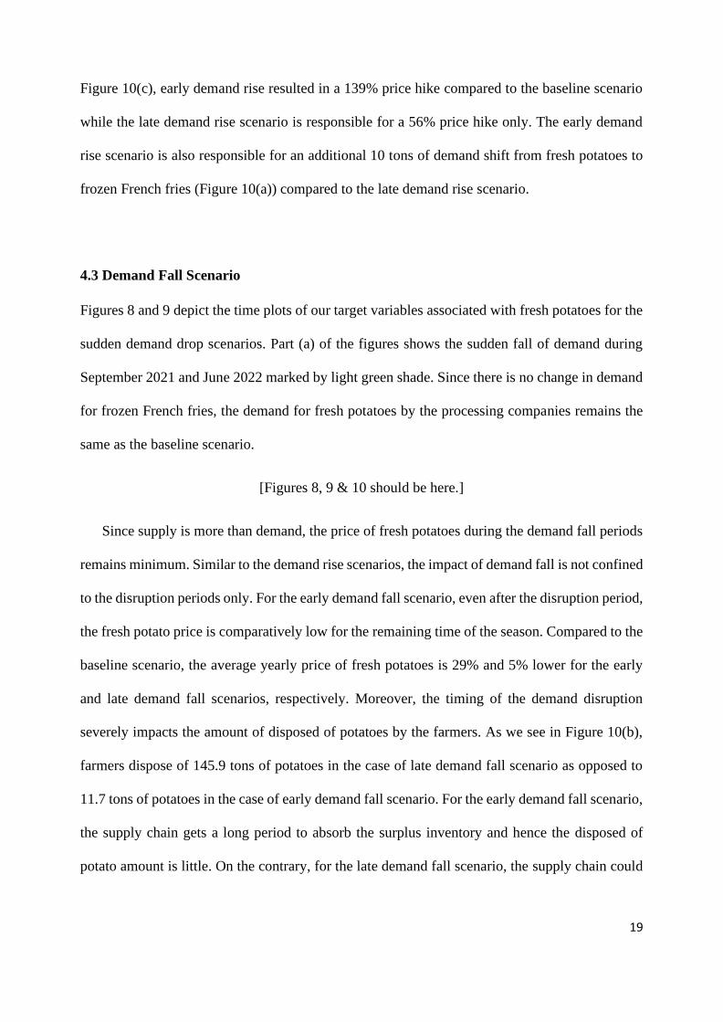
19

Figure 10(c), early demand rise resulted in a 139% price hike compared to the baseline scenario

while the late demand rise scenario is responsible for a 56% price hike only. The early demand

rise scenario is also responsible for an additional 10 tons of demand shift from fresh potatoes to

frozen French fries (Figure 10(a)) compared to the late demand rise scenario.

4.3 Demand Fall Scenario

Figures 8 and 9 depict the time plots of our target variables associated with fresh potatoes for the

sudden demand drop scenarios. Part (a) of the figures shows the sudden fall of demand during

September 2021 and June 2022 marked by light green shade. Since there is no change in demand

for frozen French fries, the demand for fresh potatoes by the processing companies remains the

same as the baseline scenario.

[Figures 8, 9 & 10 should be here.]

Since supply is more than demand, the price of fresh potatoes during the demand fall periods

remains minimum. Similar to the demand rise scenarios, the impact of demand fall is not confined

to the disruption periods only. For the early demand fall scenario, even after the disruption period,

the fresh potato price is comparatively low for the remaining time of the season. Compared to the

baseline scenario, the average yearly price of fresh potatoes is 29% and 5% lower for the early

and late demand fall scenarios, respectively. Moreover, the timing of the demand disruption

severely impacts the amount of disposed of potatoes by the farmers. As we see in Figure 10(b),

farmers dispose of 145.9 tons of potatoes in the case of late demand fall scenario as opposed to

11.7 tons of potatoes in the case of early demand fall scenario. For the early demand fall scenario,

the supply chain gets a long period to absorb the surplus inventory and hence the disposed of

potato amount is little. On the contrary, for the late demand fall scenario, the supply chain could

20

not absorb the surplus supply of potatoes within a short period. Therefore, the farmers had no

choice but to dispose of unsold potatoes before the new harvesting season starts.

4.4 Welfare Implications

In this subsection, we calculate the welfare implications for the various agents along the supply

chain. Table 2 summarizes the welfare changes for consumers, producers/retailers, and logistics

company under several demand change scenarios.

We draw several implications from table 2. First, the welfare implications for agents along the

supply chain are heterogeneous. After the demand shock, consumer and producer welfare changes

are in the same direction as the demand shocks. It should be noted that the welfare changes do

not include the social welfare from other sectors such as food services where the demand may be

shifting from. Meanwhile, logistics company delivers fewer potatoes and no potato was disposed

when there is a positive shock to the demand. When demand shrinks, logistics company delivers

more potatoes and some potatoes were disposed. Second, timing of the demand shock matters. In

fact, when the shock comes early in the production season, there would be lasting impact without

intervention. Third, policy implications for reducing food waste and mitigating welfare loss can

be vastly different.

[Table 2 should be here.]

5. Discussion

This model is meant to illustrate the effects of large shocks to consumer demand that influence

the food supply chain. This model illustrates a scenario where shocks can create food waste due to

separated supply chains, but at the same time, producer welfare can go up. This seems to be

consistent with the empirical findings of 2020. In the state of Idaho, many potato and dairy inputs

21

were wasted, but overall farm receipts increased Carlson (2021). Qualitatively, this shows us the

possible incentives for policymakers. Under reasonable assumptions, siloed supply chains may

increase expected profits. However, it will also increase the risk of producers since it increases

the variability in prices and increases the probability of wasted inputs. Siloed supply chains

might also be beneficial for some consumers if it is associated with product differentiation and

more consumer choice.

However, if food waste has associated externalities, then there may be an incentive to create

more versatility in the food supply chain or reduce the size of demand shocks.

There are a few ways policymakers might be able to mitigate the effects of large demand

shocks. Most obviously, policy restrictions on eating habits should take into account the strain

on the supply chain. More long term solutions may be standardized packaging or alleviating

restrictions on food sales. Policymakers should consider the empirical estimates of these various

costs and benefits. In some situations, there may be a need for intervention.

Similarly to increasing supply chain versatility, reducing demand shocks may decrease

profitability for firms. Since prices are bounded at zero, losses are also bounded and therefore

the effects of larger shocks are asymmetrical. However, this might change if different

distributional assumptions are made about the shocks. Nonetheless, firms may want siloed

supply chains with large demand shocks.

Mitigation Strategies and Policy Implications

While versatility may be the goal of a policymaker, it is not obvious how to increase the versatility

of these inputs. Although it may be difficult to overhaul upstream inputs, some versatility strategies

were implemented in markets. For example, some food service distributors started supplying

grocery stores. Similarly, ghost kitchens picked up some of the slack caused by supply chain

disruptions. Also, online food sales and food banks helped maintain some of the food supply. If

22

these avenues are flexible, there may be an incentive to increase the size of these types of food

sales. However, recent disruptions may also warrant changes further up the supply chain by

implementing such policies as more uniform packaging.

It is important to note, more flexible markets may also reduce market power. The trend

in food is to have differentiated food (organic, GMO, local, etc.), so while a more uniform food

supply may reduce food waste if there are large shocks to consumer demand, it may also decrease

profits. Nonetheless, it may be beneficial for policymakers to give incentives for a more versatile

food supply chain.

Reducing Demand Shocks

Aside from creating versatility in the supply chain, there are strategies to reduce shocks in

demand. The most straightforward strategies might be to limit changes in regulations and

restrictions. During the COVID-19 “lockdowns”, there were clear reasons to reduce restaurant

services. However, virus considerations may need to be balanced with food shortage

considerations if the shocks are severe.

Examples may entail limiting capacity instead of eliminating all services, making restrictions

more geographically specific, or encouraging alternatives such as drive-throughs. Also, a lack

of grocery licenses prevented some restaurants from selling directly to consumers, which would

have helped mitigate shifts in consumer demand (Linnekin 2020). Of course, these policies,

especially when initiated very quickly, can be difficult to weigh both the costs and benefits.

However, to the extent that food shortages may be a concern, an alternative to

6. Conclusion

23

This paper provides a framework to illustrate how demand shock may impact the food supply

chain, prices and food waste/shortages. Producing inputs that have versatility in the supply

chain can stabilize prices and reduce food waste. However, it is not clear that producers would

prefer siloed supply chains depending upon the differences between prices, quantities and costs.

The recent COVID-19 pandemic has illustrated the possibility of quick, large shocks to

consumer demand for virtually all types of food.

While food differentiation may alleviate some types of risk in the food supply, it can also

increase risks if consumers start to rely on certain types of food. The current food supply chain

seems to become more and more fractured with various food types such as organic food, GMOs,

local supply chains and various other attributes. This is in addition to the critical distinction of

wholesale versus retail food. Given the obvious necessity of eating and therefore the somewhat

stable aggregated demand for all types of food, a sudden shock to a segment of the food supply

can cause an enormous strain on other segments of the food supply. Therefore, this model could

potentially be used for various distinctions throughout the supply chain.

There are various mechanisms that can be used to try to remedy a lack of versatility.

Subsidization of versatility may alleviate food waste. Also, technology may be able to more

quickly adapt inputs into various outputs. Alternatively, creating more consistency in food

demand and mitigating demand shocks may also be helpful. While the food supply may be very

resilient in adjusting to long-term changes in demand Baldos and Hertel (2016), it seems less

clear in the short-run. Decisions about the food supply chain should take into account these

various costs and benefits.

24

References

Andreyeva, T., Long, M. W., & Brownell, K. D. (2010). The impact of food prices on

consumption: a systematic review of research on the price elasticity of demand for food.

American Journal of Public Health, 100(2), 216–222.

AnyLogic. (2021). AnyLogic: Simulation Modeling Software Tools & Solutions for Business.

https://www.anylogic.com/

Baldos, U. L. C. and Hertel, T. W. (2016). Debunking the ‘new normal’: Why world food prices

are expected to resume their long run downward trend. Global Food Security, 8:27–38.

Bellemare, M. F., C akir, M., Peterson, H. H., Novak, L., and Rudi, J. (2017). On the

measurement of food waste. American Journal of Agricultural Economics, 99(5):1148– 1158.

Carlson, B. (2021). Idaho net farm income surges to record high. Capital Press.

Chang, H.-H. and Meyerhoefer, C. (2020). Covid-19 and the demand for online food shopping

services: Empirical evidence from taiwan. Technical report, National Bureau of Economic

Research.

Chaudhuri, S. (2020). Comfort foods make a comeback in the coronavirus age. The Wall Street

Journal.

Craven, Teri J., and Caroline C. Krejci. 2017. “An Agent-Based Model of Regional Food Supply

Chain Disintermediation.” Pp. 1–10 in Proceedings of the Agent-Directed Simulation

Symposium.

Du, X., Lu, L., Reardon, T., and Zilberman, D. (2016). Economics of agricultural sup- ply chain

design: A portfolio selection approach. American Journal of Agricultural Economics,

98(5):1377–1388.

Ebrahimji, A. (2020). An idaho farm is giving away 2 million potatoes because coronavirus has hurt

demand. CNN.

25

Ellis, S. (2020). Idaho dairy industry encouraged by higher prices. Idaho State Business Journal.

Fang, Y. and Shou, B. (2015). Managing supply uncertainty under supply chain cournot

competition. European Journal of Operational Research, 243(1):156–176.

Gray, R. S. (2020). Agriculture, transportation, and the covid-19 crisis. Canadian Journal of

Agricultural Economics/Revue canadienne d’agroeconomie.

Hamilton, S. F. and Richards, T. J. (2019). Food policy and household food waste.

American Journal of Agricultural Economics, 101(2):600–614.

Hobbs, J. E. (2020). Food supply chains during the covid-19 pandemic. Canadian Journal of

Agricultural Economics/Revue canadienne d’agroeconomie.

Idaho Potato Commission. (2021). About Idaho Potatoes. https://idahopotato.com

Jeffery, A. and Newburger, E. (2020). Wasted milk, euthanized livestock: Photos show how

coronavirus has devastated us agriculture. CNBC.

Linnekin, B. (2020). Food issues that should’ve been front and center in the 2020 presi- dential

election. Reason.

Lusk, J. et al. (2020). Economic impacts of covid-19 on food and agricultural markets. Technical

report, Council of Agricultural Science and Technology and the Agricultural and Applied

Economics Association.

Luxen, D., & Vetter, C. (2011). Real-time routing with OpenStreetMap data. Proceedings of the

19th ACM SIGSPATIAL International Conference on Advances in Geographic Information

Systems, 513–516.

McEwan, K., Marchand, L., Shang, M., and Bucknell, D. (2020). Potential implica- tions of

covid-19 on the canadian pork industry. Canadian Journal of Agricultural Economics/Revue

canadienne d’agroeconomie.

National Potato Council. (2021). Potato Facts. https://www.nationalpotatocouncil.org/

26

Nguyen, R. T., Eggert, R. G., Severson, M. H., & Anderson, C. G. (2021). Global Electrification

of Vehicles and Intertwined Material Supply Chains of Cobalt, Copper and Nickel.

Resources, Conservation and Recycling, 167, 105198.

Rahman, Towfique, Firouzeh Taghikhah, Sanjoy Kumar Paul, Nagesh Shukla, and Renu

Agarwal. 2021. “An Agent-Based Model for Supply Chain Recovery in the Wake of the

COVID-19 Pandemic.” Computers & Industrial Engineering 158:107401.

Railsback, S. F., & Grimm, V. (2019). Agent-based and individual-based modeling: a practical

introduction. Princeton university press.

Reardon, T., Bellemare, M. F., Zilberman, D., et al. (2020a). How covid-19 may disrupt food

supply chains in developing countries. IFPRI book chapters, pages 78–80.

Reardon, T., Swinnen, J., et al. (2020b). Covid-19 and resilience innovations in food supply

chains. IFPRI book chapters, pages 132–136.

Repko, M. and Lucas, A. (2020). The meat supply chain is broken. here’s why shortages are likely

to last during the coronavirus pandemic. CNBC.

Richards, T. J. and Rickard, B. (2020). Covid-19 impact on fruit and vegetable markets.

Canadian Journal of Agricultural Economics/Revue canadienne d’agroeconomie.

Smallwood, D. M., & Blaylock, J. R. (1984). Household expenditures for fruits, vegetables, and

potatoes (No. 1488-2016-123667).

Stevenson, K. (2020). The farm-to-table connection comes undone. The New York Times.

USDA. (2020). Potatoes 2019 Summary. https://www.nass.usda.gov/

Van Voorn, George, Geerten Hengeveld, and Jan Verhagen. 2020. “An Agent Based Model

Representation to Assess Resilience and Efficiency of Food Supply Chains.” Plos One

15(11):e0242323.

Winfree, J. and Watson, P. (2017). The welfare economics of “buy local”. American Journal of

Agricultural Economics, 99(4):971–987.

Yaffe-Bellany, D. and Corkery, M. (2020). Dumped milk, smashed eggs, plowed vegeta- bles:

27

Food waste of the pandemic. The New York Times.

Yeung, J. (2020). The coronavirus pandemic could threaten global food supply, un warns.

CNN.

Zhang, X. et al. (2020). Chinese livestock farms struggle under covid-19 restrictions.

IFPRI book chapters, pages 84–85.

Zilberman, D., Lu, L., and Reardon, T. (2019). Innovation-induced food supply chain design.

Food Policy, 83:289–297.

28

Figure 1: Change in seated diners from online, phone, and walk-in reservations in the United

States from 2019 to 20201

Figure 2: Change in grocery sales in the United States from 2019 to 20202

1 Data are from https://www.opentable.com/state-of-industry. Only states or metropolitan areas with at

least 50 restaurants in the OpenTable network were included.

2 Data are from Affinity Solutions and represent “Seasonally adjusted credit/debit card spending

relative to January 4-31 2020 in grocery and food store (GRF) MCCs, 7 day moving average.”

29

Figure 3: (a) Flow of information among different agents; (b) Flow of fresh and processed potato

products at different stages of supply chain.

Legends

Fresh Potato

Processed Potato

Information

Agents

Farmers

Processors

ShippersLogistics

CompaniesGrocery Retailers

Logistics Companies

Farmers

Processors

Shippers

Logistics Companies

Grocery Retailers

(a)

(b)

Figure 4: Impact of relative humidity on potato weight loss. Source: (Olsen & Kleinkopf, 2020).

0

2

4

6

8

10

12

0 1 2 3 4 5 6 7 8 9 10 11 12

Wei

ght

loss

(%

)

Storage time (months)

100%

95%

85%

75%

30

Figure 5: Baseline scenario

31

Figure 6: Early demand rise scenario.

32

Figure 7: Late demand rise scenario.

33

Figure 8: Early demand fall scenario.

34

Figure 9: Late demand fall scenario.

35

Figure 10: (a) Amount of shifted demand from fresh potatoes to frozen French fries; (b) Amount

of disposed of potatoes by the farmers; (c) Average yearly price of fresh potatoes.

36

Table 1: Values of different parameters used in the simulation

Parameter Names Values Units Source

Number of farmer agents 6 - Assumption

Number of shipper agents 2 - Assumption

Number of processor agents 2 - Assumption

Number of logistics company agents 2 - Assumption

Number of retailer agents 3 - Assumption

Average yield of the farmlands 20 Metric

tons/acre

(USDA, 2020)

Number of farmers with contract 2 - Assumption

Number of farmers without contract 4 - Assumption

Farmland area of a farmer agent with contarct 35 – 60 Acres Assumption

Farmland area of a farmer agent without contract 150 – 180 Acres Assumption

Warehouse capacity of a shipper agent 300 – 350 Metric

tons

Assumption

Warehouse capacity of a processor agent 400 – 500 Metric

tons

Assumption

Warehouse capacity of a retailer agent 50 – 60 Metric

tons

Assumption

Daily production capacity of a processor agent 25 - Assumption

Yearly consumer demand of fresh potatoes by

consumers

2400 –

2700

Metric

tons

Assumption

Yearly consumer demand of French fries by

consumers

3300 –

3750

Metric

tons

Assumption

Number of in-house vehicles of a shipper agent 3 – 4 - Assumption

Number of vehicles owned by a logistics

company agent 10 – 15 -

Assumption

Demand elasticity of fresh potatoes - 0.58 - (Andreyeva et

al., 2010)

Relative humidity of storage facilities

95

%

(Olsen &

Kleinkopf,

2020)

37

Table 2: Welfare changes for agents along the supply chain

Scenarios Consumer surplus

change

Producer

revenue change

Logistics

company

change

Disposed

potato

amount

High demand early $4,786 $1,397 -1,289 0

Low demand early -$802 -$171 710 11.7

High demand late $2,990 $250 -388 0

Low demand late -$290 -$82 16 145.9

Notes: 1. Logistics company change is measured by the total metric tons of potatoes delivered. 2.

Consumer surplus change calculation uses the -0.58 demand elasticity in table 1.