Demixing in polystyrene/methylcyclohexane solutions

Demixing in Polystyrene/Methylcyclohexane Solutions

ATTILA IMRE' and W. ALEXANDER VAN HOOK*

Chemistry Department, University of Tennessee, Knoxville, Tennessee 37996

SYNOPSIS

Cloudpoint data for polystyrene/methylcyclohexane solutions extending over moderate ranges of pressure and molecular weight are available in the literature. Those data are supplemented with new results from this laboratory to fill in gaps and extend the MW range (to 761 5 MW/amu I 2 X lo7). The resulting data net is discussed and reasons to extend studies to higher pressure are presented. 0 1996 John Wiley & Sons, Inc. Keywords: demixing polystyrene methylcyclohexane phase equilibria consolute temperature cloudpoint closed loop molecular weight dependence pressure dependence

INTRODUCTION

The polystyrene/methylcyclohexane (PS/MCH) system is one of the most thoroughly studied polymer/solvent systems so far as demixing is concerned. PS/MCH is an example of a polymer/solvent system with both upper and lower consolute temperature curves (UCST and LCST).

Polymer/Solvent Phase Diagrams

A schematic generalized phase diagram' of the PS/ MCH type is shown in Figure la. In diagrams and throughout this work we restrict attention to liquid- liquid demixing and do not show those parts of the diagram which depict liquid/solid transitions of one kind or another including glass transitions. In Figure 1, the two-phase (shaded) regions are found at the top and bott.om centers. Figure l a shows temperature, T, plotted against concentration, $, in the plane of the figure. The third variable, which extends into the figure, might be molecular weight, pressure, or any other variable of interest. For the moment we choose the logarithm of the segment number, log(r) (proportional to log(molecu1ar weight), log(MW)). It is useful, although not completely accurate, to represent the (T, $, r) diagram as a series of coex-

* To whom correspondence should be addressed. ' Permanent address: Institute for Atomic Energy Research,

Journal of Polymer Science: Part B: Polymer Physics, Val. 34, 751-760 (1996) 0 1996 John Wiley & Sons, Inc. CCC OSS7-6266/96/040751-10

POB 49, H1525, Budapest, Hungary.

istence curves (T vs. $ at constant r ) . Four such projections (variously shaded) are sketched. As one moves into the page and toward larger and larger r, the two-phase regions increase in area. The solubility in both upper and lower branches decreases with increasing molecular weight and at high enough molecular weight, and if the solvent quality is poor enough, the two branches can eventually touch as shown in Figure Ib (these conditions we loosely label as the hypercritical point), and the system collapses into the hourglass configuration. For PS/MCH at ambient pressure, however, there is no such hypercritical point, although one might exist for solutions at negative pressure (i.e., under tension).2 At ambient pressure the homogeneous window in the center of the diagram persists to infinite molecular weight (see Fig. la).

Analysis of the phase diagram is complicated by the fact that polymer samples are polydisperse. Some points of interest are illustrated in Figure lc. Co- existing phases, while at identical temperature and pressure, are fractionated with respect to molecular weight, polydispersity, and concentration. For example, the first precipitate to form from a solution at point A on the lower (UCST) branch, (or corre- spondingly A on the upper (LCST) branch, see diagram), lies a t C (or C) , and is at a different concentration and a different segment number from the mother solution (A or A). Similarly B and D (or B' and D', upper branch), solutions which are also in equilibrium, are fractionated in both $ and MW. As a result, cloudpoint and shadow curves no longer coincide (as they do for monodisperse systems), and

75 1

752 IMRE AND VAN HOOK

(4

T

T

T

the locus of upper and lower critical points is dis- placed from the locus of maxima and minima for UCST and LCST cloudpoint curves. If polydispersity is not too high, however, the two curves may be (and often are) approximated as the same.

Much of the discussion below will refer to diagrams which project the T, locus onto the (T, r ) or (T, M,) plane. Should the homogeneous central region persist to infinite MW, TYt(rw) and T y ( r w ) define the upper and lower 0 temperatures, OLcst = T y ( r " ) and 0"Cst = TYt(ra').

Previous Demixing Studies in MCH; Comment

A good deal of information on cloudpoint loci in PS/ MCH solutions is available in the literat~re.3-l~ O b s e r ~ a t i o n s ~ ~ " ~ ' ~ ~ ~ ~ in the (T,, M,) plane establish that T;' versus (Adw)-''' is linear over a moderately wide range of MW, although according to first-order Flory theory16 this is only an approximation. One aim of the present work is to test this apparent lin- earity across a much wider range of MW. A second interesting r e s ~ l t ~ , ~ , ~ to explore is the observation that upper critical solution temperatures (UCS) projected onto the (P, T ) plane lie on a parabolic curve and define a hypercritical pressure, Pkr(UCS). At Pkr(UCS), (dT/dP), = 0 and (d2T/dP), > 0, in analogy with the low pressure hypercritical temperature, Tk,(LP) where (dP /dT) , = 0 and (d2P/dP), > 0. Towards the end of the report we raise the in-

Figure 1. Schematics for UCST/LCST demixing in (T, $, r) space. J / is the segment fraction polymer and r the segment number. The upper and lower branches of the two-phase regions are shaded. Skewing in the (T, $) plane is understood in terms of Flory-Huggins theory. The phase diagram in (T, J/ , P) space is analogous to this figure except that fractionation in P is impossible. Also P decreases as one moves across the figure. (a) For theta solutions (like methylcyclohexane/polystyrene) which show upper and lower 0 points. The inset shows the projection of the critical lines onto the (T, log(r)) plane. (b) For solutions (like acetone/polystyrene) which show upper and lower branches which join at a hypercritical point. The inset shows the projection of the critical lines onto the (T, log(r)) plane. The hypercritical point is shown as the solid circle at the center of the diagram. (c) Several sections from Fig. l a or l b chosen to illustrate the origin of MW fractionation in liquid-liquid equilibria of polydisperse polymer solutions. The equilibria shown are between A and C, A' and C', B and D, and B' and D , and are further discussed in the text. The consolute curves are flat in the region of the maxima, and the critical loci are found at nearly the same temperatures as the maxima or minima.

DEMIXING IN PS/MCH 753

triguing possibility that for certain polymer solvent systems and selected molecular weights the (T , P)cr may close to a loop, in which case two additional hypercritical conditions are defined, (1) a hypercritical pressure on the LCS branch, P,,(LCS), where (dT/dP), = 0 and (d2T/dP2), < 0, and, (2) a high pressure hypercritical temperature Thr( HP) where (dP/dT), = 0 and (d2P/dP), < 0.

Saeki and co-workers'' have reported LCSTs at different MW's. We extend those measurements to determine (P, T) loci for LCSTs in an effort to determine the sense of the curvature of this branch. Parabolic profiles of opposite sense for the UCST and LCST branches might indicate a closed T - P loop over some range of MW. That possibility has heretofore been held only the~retically,'~ but other indications do exist. For example, we have previously pointed out2 that a smooth transition from UCST to LCST exists at the low pressure end of the scale for PS/PN (PS/propionitrile) solutions, the two branches joining at a hypercritical temperature found at negative pressure. (At P = 0 and above PS/ PN displays a solubility gap at certain MWs.) There is extensive literature on the effect of pressure on the liquid-liquid transition in polymer/solvent sys-

refer- tems,l,3,5,6,19,20,24-39 many articles r 9 9

ring to polystyrene, but only a few of these3r5v6 to the PS/MCH system. High pressure measurements have been made on the UCS branch. Prior to this work no information was available on the pressure dependence of LCS demixing. Theta temperatures reported for the UCST branch for PS/MCH solutions (OUCST)P=O scatter over a 10 degree range (333.1 to 343.6 K)," but no reliable value for (OLCST)p=O was previously available. The data reported here permit the refinement of OUCsT and the definition of OLCST.

1 3 5 6 19-21,24-35

EXPERIMENTAL

Methylcyclohexane (analytical grade) was obtained from Fisher Scientific Co. and dried over molecular sieve. PS samples were obtained from Pressure Chemical Co., Pittsburgh, except for the single sample of highest MW (2 X lo7 amu) which was obtained from Scientific Polymer Products, Ontario, NY. MWs, dispersities ( M,/M,), and observed cloudpoints at or near critical concentrations are reported in Table I as are literature cloudpoint data.

Cloudpoints for low molecular weight samples (761 I M , < 2500) occur a t temperatures too low to be studied by our standard r n e t h ~ d s . ' ~ ' ~ ~ ~ ~ For samples in this MW range solutions of various concentrations approximately centered about J/hcr were

flame sealed in glass capillaries. Each sample contained a small piece of steel rod for mixing. Cloud- points were observed visually with an accuracy of about 1 K after cooling in a stirred acetone bath whose temperature was slowly lowered by dropping in bits of dry ice (in some cases additional cooling with liquid nitrogen was required). A t higher temperatures (for samples of higher MW) , cloudpoints were determined as a function of concentration, temperature, and pressure using techniques devel- oped in this l a b o r a t ~ r y . ' ~ ' ~ * ~ ~ (For M, < 2500 cloudpoints were determined by the capillary method only, for M, > 5780 by our standard technique, but for (2500 I M,/amu 5 5780) both methods were employed, and with good agreement, - 1 K or less.) In our standard method, pressure is transmitted through a mercury seal to the samples contained in a heavy wall glass capillary and the transition de- tected by small-angle light scattering with f O . l K or better precision. For PS30,000, PS90,000, and PS1,971,000 critical concentrations were obtained from the literature and P , T isopleths determined at that concentration only. Samples of PS20,000,000 were prepared at three concentrations between 1 and 2 wt 9%. Errors from thermal degradation were smaller than 1 K on the LCST and negligibly small on the UCST branch.

RESULTS

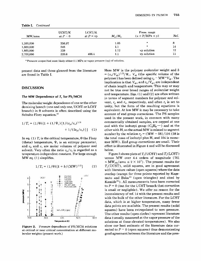
Figure 2 shows the present results on the pressure dependence of cloudpoints of upper and lower branches for samples of near critical composition. We have extrapolated these results to zero pressure and entered the results in Table I. The pressure dependence of UCST is small and the difference between UCST ( P = 0) and UCST ( P = solution vapor pressure) is negligible. Figure 2 and Table I1 show that as MW falls UCST drops to lower temperature but LCST increases. ( dT/dP),,p=o, negative and small at high MW in the UCST branch, becomes even smaller in magnitude as MW decreases, eventually crossing zero and becoming positive at the lowest MW studied. We will return to this point later in the discussion. For the LCST branch (dT / d P ) is positive at all MWs we studied.

( T , J / ) diagrams are flat in the region of the max- imum. Along with others3,4,7,8,'0-'3 we have elected to use the maxima of ( T , $) curves to represent T,; errors introduced by this approximation do not ex- ceed a few tenths K for these solutions with low Mw/ M,. Critical temperatures obtained from the


Table I. of PS/MCH solutions

Molecular Weight Dependences of Upper and Lower Critical Solution Temperatures

UCST/K LCST/K Press range Conc. range MW/amu a t P = O a t P = O Mw/MIz ( x I P/MPa I y ) w t %

Present work 761 1241 1681 2500 4000 5780 30,000 90,000 1,971,000 20,000,000

MW/amu

189 214 230 246 261 271 302

336 343

UCST/K a t P = O

1.14 1.07 1.06 1.09 1.06 1.05

497 1.03 490 1.04 476 1.26 470 1.2

LCST/K a t P = v p M J M ,

x , Y vp solution vp solution vp solution

0.1, 5.1 0.1, 4.8 0.2, 5.0 0.1, 5.3 2.3, 4.4 0.1, 6.0 0.2, 4.9

Press. range ( x 5 P/MPa I y )

18-31 16-39 20-39 19-43 15-34 13-36

20 13 2

1-2

Ref.

Literature results 9000 9000 10,200 10,200 13,000 16,100 16,100 17,200 17,300 17,500 17,500 20,200 22,000 23,000 28,500 29,000 34,900 34,900 37,000 37,000 46,400 50,000 97,200 97,200 109,000 110,000 181,000 200,000 233,000 233,000 400,000 411,000 670,000 719,000 719,000 860,000 900,000

279 281 285.7 285.71 291.3 296 295.98 296.7 296.13 297 296.32 298.95 301 302.2 305 306.1 309 309 309.65 309.7 312.61 313 321.8 318.1 322.71 323.34 327.0 327.4 329.92 330 332.7 344.0 334.5 334.8 334.82 346.3 336

515.8

505.9

499.9

496.4

492.3

1.06 1.06 1.06 1.06 1.06 1.06 1.06

< 1.06 1.06 1.06 1.06 1.06 1.03 1.06 1.1 1.06 1.06 1.06 1.06 1.06 1.06 1.06 1.06 1.1 1.06 1.06 1.06 1.06 1.06 1.06 1.06 1.1 1.1

< 1.06 1.06 1.1 1.1

x, Y 0.1, 90

0.1, 80

vp solution 0.1, 80

a

23

B

B

a

0.1, 90 a

a

0.1, 70 vp solution

0.1, 90 vp solution

0.1, 80 a

a

vp solution

0.1, 90 vp solution

a

a

a

a

a

vp solution

vp solution vp solution

vp solution a

a

a

vp solution

3 8 5 7, 10 4 5 7, 10 13 7, 10 3 8 7, 10 6 4 3 4 5 7, 10 8 11 7, 10 3 11 14 7, 10 8 7, 10 11 8 12 11 14 11 13 7, 10 14 12


Table I. Continued

UCST/K LCST/K Press. range MW/amu a t P = O a t P = v p M J M l (z I P/MPa I y ) Ref.

1,260,000 1,800,000 1,860,000 2,700,000

a 8 336.97 1.05 348 1.1 339 1.12 vp solution 12 339.6 488.4 1.1 vp solution 11

B 14

* Pressure unspecified most likely either 0.1 MPa or vapor pressure (vp) of solution.

present data and those gleaned from the literature are found in Table I.

Here MW is the polymer molecular weight and b = (u,/Vsp) 1/2/*1. V, (the specific volume of the polymer) has been defined using up = MW * V, . The implication is that V,, and u,/Vsp, are independent of chain length and temperature. This may or may not be true over broad ranges of molecular weight

DISCUSSION

The MW Dependence of 1, for PS/MCH and temperature. Eqs. ( 1 ) and ( 2 ) are often written in terms of segment numbers for polymer and sol-

The molecular weight dependence of one or the other demixing branch (one and only one, UCST or LCST branch) in 0 solvents is often described using the Schultz-Flory equation.16

vent, rp and rs, respectively, and often rs is set to unity, but the form of the resulting equations is equivalent. At low MW it may be necessary to take account of end group corrections. The PS samples used in the present work, in common with many

In eq. ( 1 ) T, is the critical temperature, 0 the Flory (theta) temperature, \kl is an entropy parameter, and up and us are molar volumes of polymer and solvent. Very often the ratio u,/u, is regarded as a temperature-independent constant. For large enough MW eq. ( 1) simplifies.

1/T, = (1 /@)[1 + b/(MW)'I2] ( 2 )

commercially obtained samples, are capped at one end with the isobutyl group ( C4H9- ) and at the other with H, so the actual MW is related to segment number by the relation rp = (MW - 58) / 104 (58 is the total mass of isobutyl plus H, and 104 is mono- mer MW) . End group corrections are small. Their effect is illustrated in Figure 4 and will be discussed below.

Figure 3 shows plots of T, (UCST) and T, (LCST) versus MW over 4.4 orders of magnitude (761 I MWps/amu I 2 X l o7 ) . The present results for T, (UCST) , solid squares, are in good agreement with literature values (open squares) where the data overlap (except for three points reported by Kage-

~ W PS4.000 9 mot0 and Baba14 (open triangles) and cited by ---+-- PS30.000 Kamide21). All measurements have been corrected --+- . PS1.971.000 Ps20,000,000 -r ' to P = 0 (but for the UCST branch that correction

is small or negligible). We offer no reason for the inconsistency of ref. 14 with the present results and with the bulk of the other literature. For the LCST data, which is at higher temperature, many fewer data points are available. The present results (solid

, 9/ solubilitygop squares ) have been extrapolated to zero pressure. The other results (open circles) represent literature

200 300 400 500 660 data (usually measured at the vapor pressure of the solutions at these elevated temperatures). We also show our best estimate of the literature data corrected to P = 0 (open squares) thus demonstrating good agreement between the literature and the pres-

- - - 8 - - PS2.500 LCST

- *- ~ PS5.600 6 - UCST

J - " r

3 -

m r b ; ,+ 2 - j t; !

i' / / !, " I / ; I, 0 ,

Temperature (K)

~i~~~ 2. pressure dependence of PS/MCH so~utions at critical or near critical concentration at different molecular weights (present work.)


Table 11. in Table I P = A. + A,T + A2T2 + A3T3 + A4T4

Empirical Constants in Fitting Relations Describing (T, P) Loci of the Data

MW Branch, range A0 A1 A2 ~o*A, lo7&

2500 ucst, 243.0-243.4 -1176.628 4.831911 4000 ucst, 259.8-260.4 624.789 -2.395307 5780 ucst, 270.8-271.1 4220.95 - 15.56868 30,000" ucst, 297.5-301.4

Icst, 514.9-529 4182.764 -37.48829 0.1229218 -1.762317 0.9376541 90,000 lcst, 507-523 -64.73212 0.1321428 1,97 1,000" ucst, 333.1-335.5

h i t , 486.8-521.1 14824.59 -131.476 0.431851 -6.244502 3.361623

h t , 483.2-508.3 11830.83 -104.6453 0.3436162 -4.977118 2.688846 20,000,000" ucst, 339.7-343.7

a This polynomial fit includes both branches and extends into the range of negative pressure where it displays very little reliability because no experimental data exist for these samples in that pressure range.

ent results. To make the corrections smoothed Val- ues for d P / d T taken from Figure 2 were employed. We were unable to measure T,(LCST) for MWs below 30,000 or so because the temperatures become too high. Relationships Between Pressure

Figure 4 shows the T,s from Table I corrected to

Good straight lines are observed and the parameters of fit reported in Table 111.

and Solvent Quality zero pressure and plotted according to eq* ( used eq- ( data exist defining the

). We ) because no accurate

and Mw dependence Of vsp*

The discussion of pressure and solvent quality which follows may be clarified by reference to Figure 5a and b. It is well known that the solubility gap of

rather than eq* (

The data Once corrected for end effects (vide supra) = (o( LCST) - o( UCST ) ) , is are shown as the "lid The correction pressure sensitive (e.g., see ref. 24); usually elevated

MW. Data from ref. 14 are not included in the plot. one in the direction of better

theta solvents,

is important only for the Or Of lowest pressures cause an increase in A@, ip., increasing the pressure solvent quality. Conversely decreasing the pressure, or lowering solvent quality, moves in the direction

500 1 A

v Y

g 400

1 0 0 ~ ' ' ' ' " ' """" ' " """ ' " " " " ' """" ' ' i 03 104 105 106 i 07

Molecular weight (amu)

Figure 3. Molecular weight dependence of upper and lower consolute temperatures for PS/MCH solutions (Table I). The upper and lower dashed lines represent the liquid/vapor critical temperature and the freezing temperature of pure MCH, respectively. The choice of the logarithmic scale for MW is for convenience. Present data ( P = 0). 0 Literature data (corrected to P = 0). 0 Literature data, LCST branch, uncorrected. A Data from ref. 14.

0.04 1

I 0.03

Figure 4. Schultz-Flory representation of UCST and LCST demixing data for PS/MCH at P = 0. Present data (P = 0). 0 Literature data (corrected to P = 0). 0 Present data corrected for end effects (correction is only noticeable for the four data points of lowest MW). - least-squares line for uncorrected data, see Table 111. ----- least-squares line for corrected data, see Table 111.


Table 111. Least-Squares Fits of UCST and LCST Loci for MCH/PS Solutions

Without End Corr. With End Corr.

Parameter Eq. (2) Table IV Eq. (2) Literature

e.-t/K 344.6 345.0 343.5 331 to 343.6 eteet/K 470 464.5 - 484 (473 at P = 0) buCst 21.5 - 20.8 20.2 bIC8t -9.97 - - -

of decreasing A@. If the pressure is low enough the gap can go to zero as shown for the intermediate case in Figure 5a. At a yet lower pressure, one might say the solvent has been transformed from a theta to a non-theta solvent. This might happen at a negative pressure (i.e., when the solution is under tension ).

For some systems, such as PS/acetone and PS/ DMCP (dimethylcyclopentane) , the UCST and LCST branches join at ambient pressure and finite molecular weight ',20*22 ( i.e., the two branches meet at a hypercritical point ) . The solvent cannot dissolve polymer of MW greater than the hypercritical molecular weight, MWh,,, at that pressure. On the other hand, increasing pressure is equivalent to increasing solvent quality; thus it is possible to transform some non-theta solvents into theta solvents by increasing the pressure above a certain critical value, Pg (hcp) . Pg (hcp) is the minimum pressure where the solvent will dissolve polymer of infinite molecular weight, and AQ = 0. For P > P g (hcp) the solvent is better yet, and AQ > 0. In effect one is using pressure to titrate solubility along the UCST/ LCST critical locus (i.e., using it to change solvent quality a t constant solvent composition).

It is also possible to titrate solubility a t constant pressure by varying solvent quality (i.e., composition). For example, methylcyclopentane at ambient pressure is a theta solvent for PS but its perdeuter- oisomer is not.' Thus one expects to find a mixed solvent x M C p ( h ) / ( 1 - x ) M C p ( d ) such that Pg (hcp) = 0. This is no surprise. The whole area of controlled MW fractionation and the purification of many polymers depends on the adjustment of solvent quality in mixed solvents, i.e., varying the composition ratio of solvent and cosolvent to selectively precipitate polymers of high end MW. (But there is no reason to expect a linear relation between solvent composition and solvent quality. For example both acetone and n-alkanes are poor solvent^,'^ but an acetone /alkane mixture is better than either pure component; excess effects may be important and can even dominate.)

The paragraphs above argue that it may be useful to consider the UCST/LCST phenomena as common manifestations of a single cause. Toward that end we have chosen a description which uses a single polynomial to fit critical loci from both branches. Figure 6 illustrates a fit of UCST and LCST (Table I ) with a fourth-degree polynomial. The parameters are reported in Table IV. Figure 6 is strictly analogous to the schematic (Fig. 5b). For 0 solvents (like MCH) the fit of the zero pressure data has its minimum at negative 1 / M t / 2 . This has parametric, not physical, meaning; M i l l 2 is not defined in the (+, - ) quadrant. Of course Figure 5b indicates that, if we could lower the pressure far enough, the hypercritical condition could be moved into the ( +, + ) quadrant and a physically meaningful hypercritical MW defined, most likely in the region of negative pressure.

Determination of Q Temperatures

Theta temperatures obtained from fits to eq. ( 2 ) are reported in Table 111. We, however, prefer polynomial fits to both branches (vide supra) , which are found in Table IV. The fourth-order fit shown in Figure 6 yields Q( UCST) = 345 K which compares nicely to the linear fit [ eq. ( 1 ) 1, 344.6 K ( 343.5 K if end corrections are included). The value is a little larger than the highest of the commonly tabulated values18 which range between 333.1 and 343.6 K (333.1, 340.3, 341.1, 343.6 K ) .

Larger differences are found for the LCST branch. Thus we obtain Q( LCST) , eq. ( 1) = 470 K, and Q( LCST, 4th-order poln.) = 464.5 K. The only literature result is due to Saeki et al." who report Q(LCST, P = vap. press) = 484 K, which, when corrected by us to zero pressure, gives Q( LCST, P = 0) = 473 K, in reasonable agreement with the present results. Remember that Q( LCST) is much more pressure sensitive than @( UCST) . We also observed the b parameters, eq. (2 ) . The previously reported best value for bUCsT is 20.2 based on measurements extending between lo5 and 7 X lo5 amu.


0.04

0.03

0.02

0.01

0.00

I \ I I P3 > P2 > Pl -

-

-

-

___-_----.

Figure 5. Schematic representations of the dependence of (TJMW) demixing curves on pressure (a) and solvent quality (b). The outermost curves are typical for good quality (b) or high pressure (a) @-solvents. Upper and lower demixing branches are observed. The intermediate curve shows A@ = 0 a t infinite MW, the inner curves (poor solvent quality (b), low or perhaps negative pressure (a)) show more limited solubility.

The present fit yields b = 21.5 (20.8 with end corrections included) and is based on measurements extending from 761 to 20 X lo6 amu. We find bLsCT

= -9.97. No previous result is available.

A Closed P - T loop?

In previous measurements on propionitrile / PS2 we showed the solubility gap at finite molecular weight, T, (LCST) - T, (UCST) , disappears at low enough pressure. The two branches join at a hypercritical point found at negative pressure. The ( P , T ) iso-

? \

i \1 \

\

500 -0.01 '

100 200 300 400 T(K)

Figure 6. Polynomial representation of UCST and LCST demixing data for PS/MCH at P = 0. The parameters which describe the fit (curved dashed line) are reported in Table IV. The horizontal line represents infinite molecular weight.

pleths in the neighborhood of Thr( LP) are concave parabolic (see Fig. 7 ) . Although no information on demixing at negative pressure is available for MCH/ PS, we expect it to display the same general features as PS/PN.

Now consider the behavior of UCST and LCST as P increases at constant molecular weight and constant solvent composition. The information (Table I ) for LCST extends to only 5 MPa, or so, and is not precise enough to define d 2 T / d P 2 in this region of the diagram. (The data are represented by the heavy solid line at the right side of Figure 7; we are unable to determine whether it continues concave parabolic or is now linear, or even convex in the ( T , P ) projection). On the other side of the diagram, however, the literature data for UCST extend to 100 MPa or so3p5s6 and definitely show that d T / d P goes through zero at some tens of MPa's (for = lo4 I MW/amu 5 l o5 ) . The present data qualitatively confirm this behavior but the pressure range is not large enough to permit useful quanti- tative comparisons. The point of interest is that a hypercritical pressure, Phr(UCS), (dT/dP)Ucs = 0, (d2T/dP2)"Cs > 0, exists at some point along the

Table IV. (Mi1/ ' , T)p=o Loci

Empirical Least Squares Constants for

Mi1/' = Bo + BIT + B2T2 + B3T3 + B4T4 (8 X 10' < M,/amu < 2 X 10')

0.1 189 158 -5.518922 X

7.168329 X

1.36884 X -8.142638 X lo-''


*.#--,'

T d W T Figure 7. Hypothetical closed (P, r ) demixing loops at several molecular weights consistent with available information on PS/MCH solutions. The diagram is discussed a t length in the text. Some lines or parts of lines are hypothetical. The sections supported by known data are represented as the heavy solid lines. The polynomial description (Table IV) predicts THCR(LP) where ( ( d P / d T ) , = 0 and (d2P/dP) , > 0) at negative pressure. Observed curvature in UCST isopleths at low enough MW dem- onstrates the existence of PHcR(UCS) where (dT/dP), = 0 and (d2T/dP2), > 0. It is possible (see Discussion) that a closed loop may exist, (medium weight dashed line). Al- ternatively, the P, T demixing locus may be open (light continuous lines). Supposing a closed (P, r ) demixing loop exists, we show expected MW dependences with the solid lines at lower and higher MW.

UCS branch, for a t least some molecular weights. With the existence of the low pressure hypercritical temperature and the UCS hypercritical pressure both established, it becomes interesting to consider the possibility of a closed ( P , T )CR loop such as the one sketched in as the dashed line in Figure 7. Ex- perimental confirmation will require pressure control extending from well into the negative region to rea- sonably high pressures, say on the order of 200 MPa, and awaits investment in new instrumentation.

Schneider l7 has pointed out the theoretical possibility of closed-loop behavior, but to our knowledge no example has yet been found for polymer/solvent solutions. Even so, examples do exist of systems which exhibit either a high or low pressure hypercritical temperature, Thr( HP) or T&,( LP) (see Fig. 7 ) , or a hypercritical pressure on the UCS branch, Phr(UCS) (i.e., three of the four possible hypercritical points are known). Thus acetone/PS (MW = 22000) shows Th,(LP) ( ( d P / d T ) , = 0 and ( d 2 P /

dT2), > 0) a t low positive For propionitrile/PS (MW = 22000) solutions Th,(LP) is found at negative pressure.2 We have already pointed out that MCH /PS solutions show a hypercritical pressure on the UCS branch, Pkr( UCS) , ( (dT/dP), = 0 and ( d2T/dP2) , > O ) , somewhere around 30 to 50 Mpa?r6 Finally some small molecule systems display high pressure hypercritical temperatures, Th,( HP ) , (dP /dT) , = 0 and ( d2P/dT2) , < 0, ethylene/toluene is a notable example.*' It thus seems reasonable to anticipate that a careful search may result in the identification of a hypercritical pressure on an LCS branch, Ph,(LCS) ( (dT /dP) , = 0 and (d2T/dP2)r < 0) , in some solutions, and perhaps a closed loop. Because two hypercritical points have already been identified in MCH/PS, it seems plausible to search there for closed loop behavior.

It is interesting to consider the expected MW dependence of a closed-loop diagram. It is experimen- tally established that P,,(UCS) increases with MW3f5s6 in PS/MCH solutions. The exact form of the dependence is not established, but result^^.^.^ indicate Phc,(UCS) is probably negative at small MW (see the dashed line in Fig. 7). This is to imply (dP(UCS)/dT)+, > 0 for small enough MW (usually (dP(UCS)/dT),=, < 0). For PS2500/MCH we found (Table I1 and Fig. 2) that cloudpoint temperatures at some concentrations and P = 0 are smaller than the ones at 5 MPa (vide supra), again indicating (dP(UCS)/dT) < 0, but the differences are small compared to the precision of the measurements. Nonetheless, summing up, the arguments discussed above taken as a whole indicate a real possibility for the existence of a closed (P, vcR loop in PS/MCH solutions. The existence of such a loop has interesting theoretical and practical consequences.

CONCLUSIONS

Temperature/MW loci for critical demixing in PS / MCH solutions have been shown to display a smooth orderly dependence over 4.4 orders of magnitude and can be described usefully with either a single polynomial representation, or separate Schultz-Flory representations for the UCST and LCST branches. The @-temperatures and b parameters for PS/MCH so determined are in good agreement with previously reported data, a t least where comparisons are possible. Pressure dependences for both branches have been determined, that for LCST for the first time. The curvature in ( T,, MW) and ( T,, P ) sections of the PS/MCH phase diagram have been discussed


and the possible existence of a closed ( P , T) loop in this system has been pointed out.

This work was supported by the U. S. Department of En- ergy, Division of Materials Sciences.

20. J. Szydlowski and W. A. Van Hook, Macromolecules, 24,4883 (1991).

21. K. Kamide, Thermodynamics of Polymer Solutions. Phase Equilibria and Critical Phenomena, Polymer Science Library v. 9, Jenkins, A. D., ed. Elsevier, Am- sterdam, 1990.

22. J. M. G. Cowie and I. J. McEwen, Polymer, 25,1107 (1984).

23. J. M. G. Cowie and I. J. McEwen, Polymer, 24,1449 REFERENCES AND NOTES

1.

2.

3.

4.

5.

6.

7.

8.

9.

10.

11.

12.

13.

14.

15.

16.

17.

18.

M. Luszczyk, L. P. N. Rebelo, and W. A. Van Hook, Macromolecules, 2 8 , 745 ( 1995). A. Imre and W. A. Van Hook, J . Polym. Sci., Polym. Phys., 32B, 2283 (1994). S. Vanhee, F. Kiepen, D. Brinkmann, W. Borchard, R. Koningsveld, and H. Berghmans, Macromol. Chem. Phys., 195 , 759 (1994). W. Shen, G. R. Smith, C . M. Knobler, andR. L. Scott, J . Phys. Chem., 95,3376 (1991). H. Hosokawa, M. Nakata, andT. Dobashi, J. Chem. Phys., 98,10078 (1993). P. A. Wells, Th. W. de Loos, and L. A. Kleintjens, Fluid Phase Equilibria, 83, 383 (1993). T. Dobashi, M. Nakata, and M. Kaneko, J. Chem. Phys., 72,6685 (1980). K. Shinozaki, T. Van Tan, Y. Saito, and T. Nose, Polymer, 23, 728 (1982). K. Shinozaki, T. Hamada, and T. Nose, J . Chem. Phys., 77,4734 (1982). T. Dobashi, M. Nakata, and M. Kaneko, J . Chem. Phys., 72,6692 ( 1980). S. Saeki, N. Kuwahara, S. Konno, and M. Kaneko, Macromolecules, 6, 246 (1973). B. Chu, K. Linliu, P. Xie, Q. Ying, Z. Wang, and J. W. Shook, Rev. Sci. Instrum., 62,2252 (1991). T. Dobashi, M. Nakata, and M. Kaneko, J. Chem. Phys., 80,948 ( 1984). K. Kagemoto and Y. Baba, Kobumshi Kagaku, 2 8 , 784 (1971). B. Chu and Z. Wang, Macromolecules, 21, 2283 ( 1988). P. J. Flory, Principles of Polymer Chemistry, Cornell University Press, Ithaca, NY, 1953. G. Schneider, Ber. Bunsenges. Physik. Chem., 70,497 (1966). H. G. Elias, in Polymer Handbook, 3rd ed., J. Brandrup and E. H. Immergut, Eds., John Wiley & Sons, New York 1989, VII/205.

( 1983). 24. S. Saeki, N. Kuwahara, and M. Kaneko, Macromol-

ecules, 9,101 (1976). 25. S. Saeki, N. Kuwahara, K. Hamano, Y. Kenmochi,

and T. Yamaguchi, Macromolecules, 19,2353 ( 1986). 26. L. Zeman and D. Patterson, J. Phys. Chem., 76,1214

( 1972). 27. B. A. Wolf and H. Geerissen, Colloid & Polym. Sci.,

259,1214 (1981). 28. J. R. Schmidt and B. A. Wolf, Colloid & Polym. Sci.,

257,1188 (1979). 29. M. Nakata, S. Higashida, N. Kuwahara, S. Saeki, and

M. Kaneko, J. Chem. Phys., 64,1022 (1976). 30. C. D. Myrat and J. S. Rowlinson, Polymer, 6 , 645

(1965). 31. F. Kiepen and W. Borchard, Makromol. Chem., 189,

2595 (1988). 32. F. Kiepen and W. Borchard, Macromlecuks, 21,1784

(1988). 33. M. Ishizawa, N. Kuwahara, M. Nakata, W. Nagayama,

and M. Kaneko, Macromolecules, 11,871 ( 1978). 34. J. S. Ham, M. C. Bolen, and J. K. Hughes, J . Polym.

Sci., 57 , 25 (1962). 35. S. Saeki, N. Kuwahara, M. Nakata, and M. Kaneko,

Polymer, 16,445 (1975). 36. M. A. LoStracco, S. H. Lee, and M. A. McHugh, Poly-

mer, 35,3272 (1994). 37. S. J. Chen, I. G. Economou, and M. Radosz, Fluid

Phase Equilibria, 83, 391 ( 1993). 38. S. H. Lee, M. A. LoStracco, and M. A. McHugh, Mac-

romolecules, 2 7 , 4652 (1994). 39. L. Zeman, J. Biros, G. Delmas, and D. Patterson, J.

Phys. Chem., 76,1206 (1972). 40. B. M. Hasch and M. A. McHugh, Fluid Phase Equi-

libria, 6 4 , 251 (1991).

Received June 13, 1995 19. J. Szydlowski, L. P. Rebelo, and W. A. Van Hook, Revised August 8, 1995

Accepted September 18, 1995 Rev. Sci. Instrum., 63, 1717 (1992).

Documents

Demixing in polystyrene/methylcyclohexane solutions