DEMON: Mining and Monitoring Evolving Data

Venkatesh GantiUW-Madison

Johannes GehrkeCornell University

Raghu RamakrishnanUW-Madison

Presented byNavneet Panda

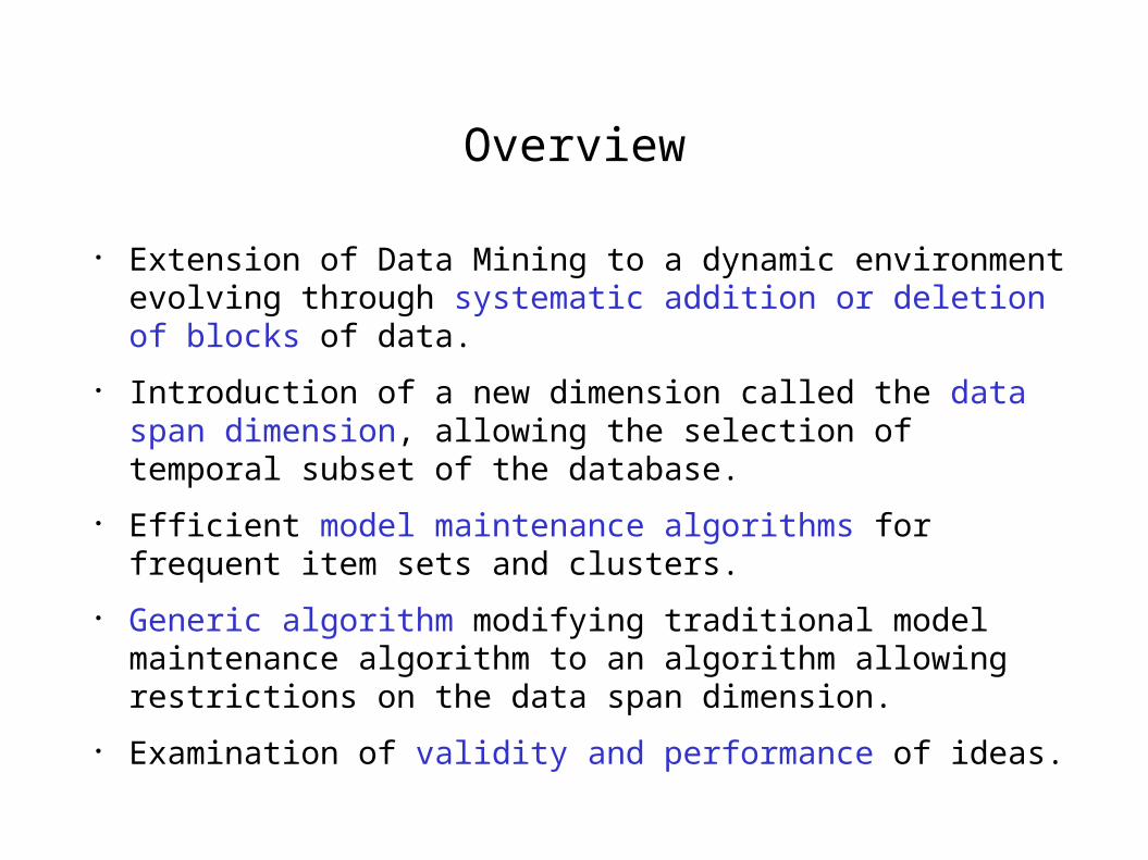
Overview

● Extension of Data Mining to a dynamic environment evolving through systematic addition or deletion of blocks of data.

● Introduction of a new dimension called the data span dimension, allowing the selection of temporal subset of the database.

● Efficient model maintenance algorithms for frequent item sets and clusters.

● Generic algorithm modifying traditional model maintenance algorithm to an algorithm allowing restrictions on the data span dimension.

● Examination of validity and performance of ideas.

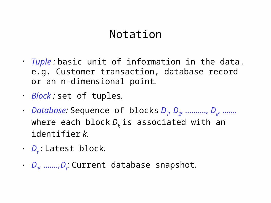
Notation

● Tuple : basic unit of information in the data. e.g. Customer transaction, database record or an n-dimensional point.

● Block : set of tuples.

● Database: Sequence of blocks D1, D

2, .........., D

k, ....... where each

block Dk is associated with an identifier k.

● Dt : Latest block.

● D1, .......,D

t: Current database snapshot.

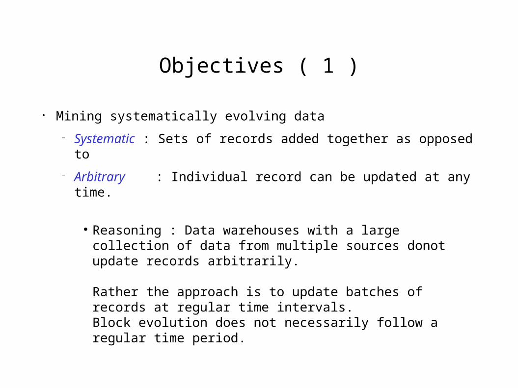
Objectives ( 1 )

● Mining systematically evolving data

– Systematic : Sets of records added together as opposed to

– Arbitrary : Individual record can be updated at any time.

● Reasoning : Data warehouses with a large collection of data from multiple sources donot update records arbitrarily.

Rather the approach is to update batches of records at regular time intervals. Block evolution does not necessarily follow a regular time period.

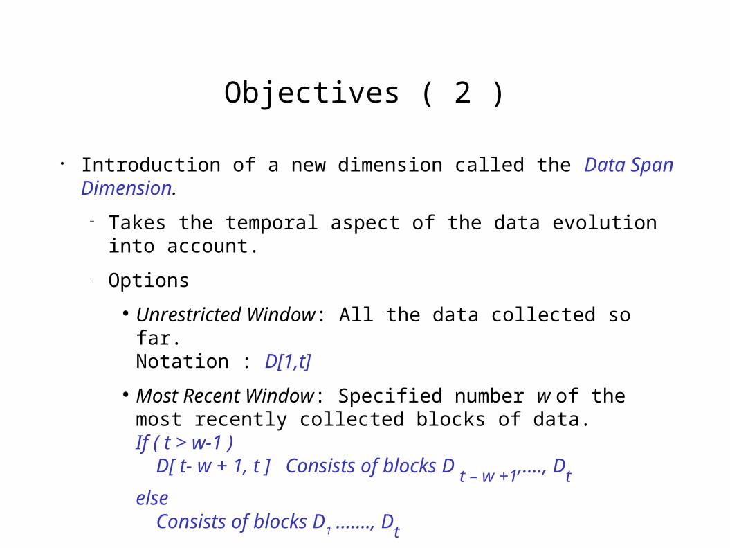
Objectives ( 2 )

● Introduction of a new dimension called the Data Span Dimension.

– Takes the temporal aspect of the data evolution into account.

– Options

● Unrestricted Window: All the data collected so far. Notation : D[1,t]

● Most Recent Window: Specified number w of the most recently collected blocks of data.If ( t > w-1 ) D[ t- w + 1, t ] Consists of blocks D

t – w +1,...., D

telse Consists of blocks D

1 ......., D

t

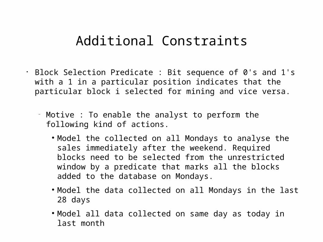
Additional Constraints

● Block Selection Predicate : Bit sequence of 0's and 1's with a 1 in a particular position indicates that the particular block i selected for mining and vice versa.

– Motive : To enable the analyst to perform the following kind of actions.

● Model the collected on all Mondays to analyse the sales immediately after the weekend. Required blocks need to be selected from the unrestricted window by a predicate that marks all the blocks added to the database on Mondays.

● Model the data collected on all Mondays in the last 28 days

● Model all data collected on same day as today in last month

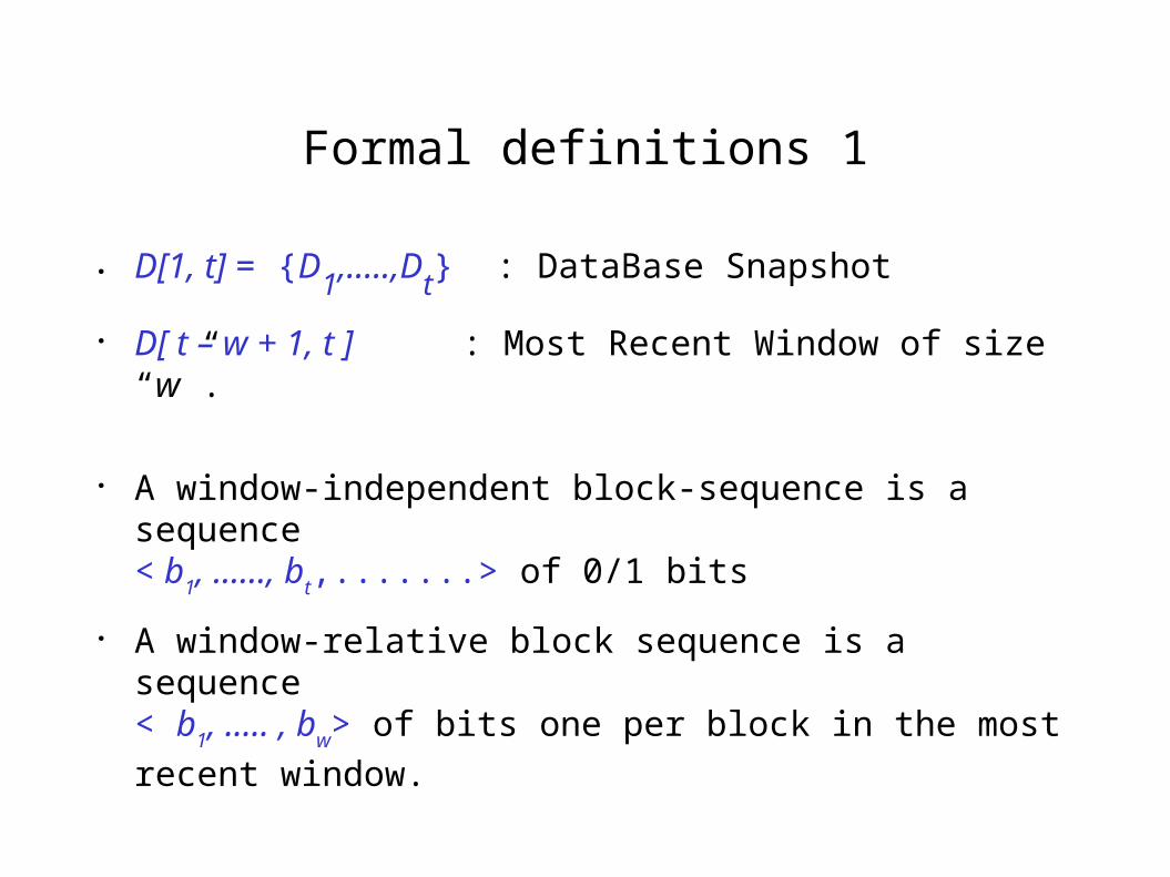
Formal definitions 1

● D[1, t] = {D1,.....,D

t} : DataBase Snapshot

● D[ t – w + 1, t ] : Most Recent Window of size “w”.

● A window-independent block-sequence is a sequence< b

1, ......, b

t,.......> of 0/1 bits

● A window-relative block sequence is a sequence< b

1, ..... , b

w> of bits one per block in the most recent window.

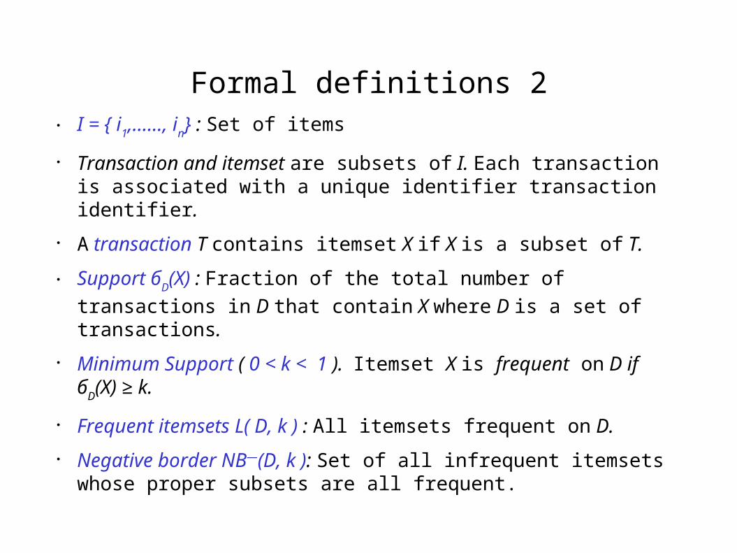
Formal definitions 2● I = { i

1,......, i

n} : Set of items

● Transaction and itemset are subsets of I. Each transaction is associated with a unique identifier transaction identifier.

● A transaction T contains itemset X if X is a subset of T.

● Support бD(X) : Fraction of the total number of transactions in D

that contain X where D is a set of transactions.

● Minimum Support ( 0 < k < 1 ). Itemset X is frequent on D if б

D(X) ≥ k.

● Frequent itemsets L( D, k ) : All itemsets frequent on D.

● Negative border NB—(D, k ): Set of all infrequent itemsets whose proper subsets are all frequent.

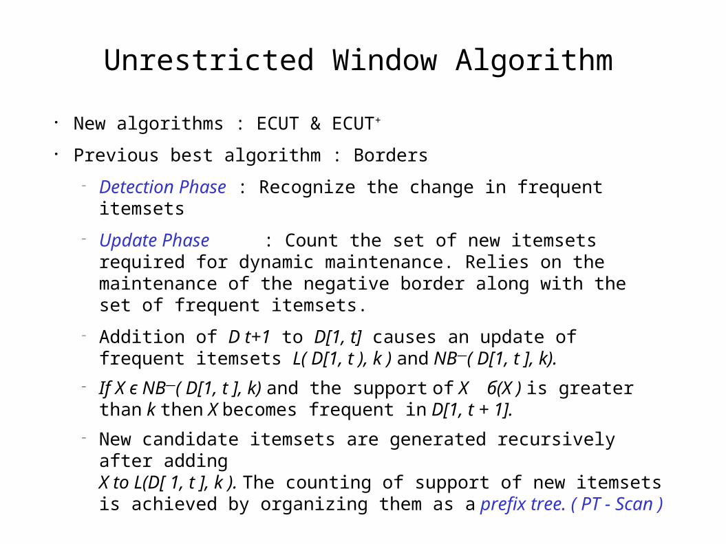
Unrestricted Window Algorithm

● New algorithms : ECUT & ECUT+

● Previous best algorithm : Borders

– Detection Phase : Recognize the change in frequent itemsets

– Update Phase : Count the set of new itemsets required for dynamic maintenance. Relies on the maintenance of the negative border along with the set of frequent itemsets.

– Addition of D t+1 to D[1, t] causes an update of frequent itemsets L( D[1, t ), k ) and NB—( D[1, t ], k).

– If X є NB—( D[1, t ], k) and the support of X б(X ) is greater than k then X becomes frequent in D[1, t + 1].

– New candidate itemsets are generated recursively after adding X to L(D[ 1, t ], k ). The counting of support of new itemsets is achieved by organizing them as a prefix tree. ( PT - Scan )

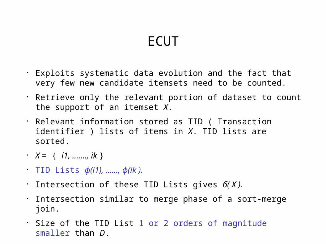
ECUT

● Exploits systematic data evolution and the fact that very few new candidate itemsets need to be counted.

● Retrieve only the relevant portion of dataset to count the support of an itemset X.

● Relevant information stored as TID ( Transaction identifier ) lists of items in X. TID lists are sorted.

● X = { i1, ......., ik }

● TID Lists ф(i1), ......, ф(ik ).

● Intersection of these TID Lists gives б( X ).

● Intersection similar to merge phase of a sort-merge join.

● Size of the TID List 1 or 2 orders of magnitude smaller than D.

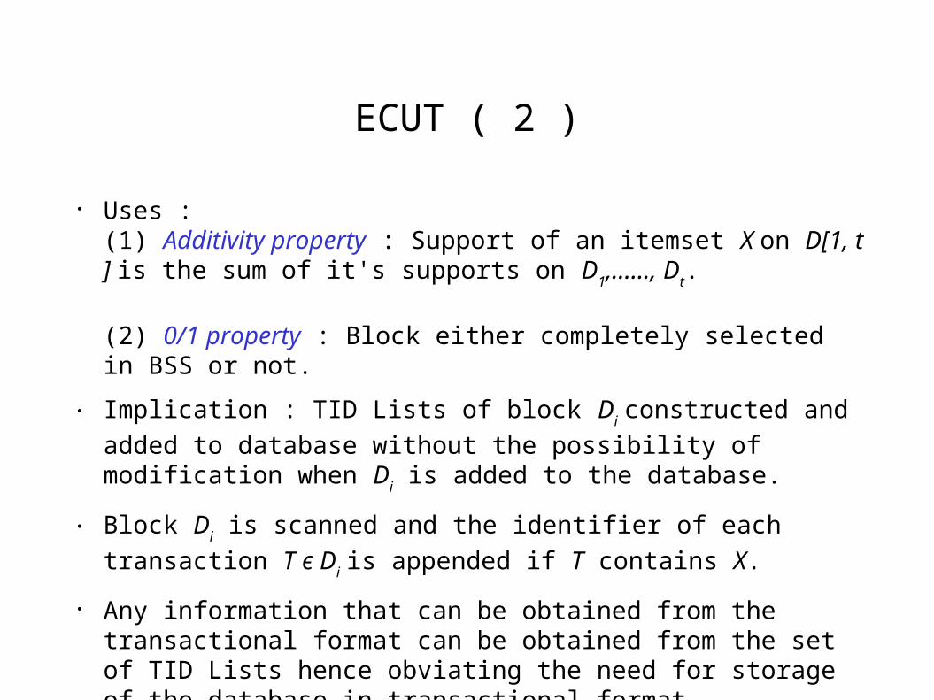
ECUT ( 2 )

● Uses : (1) Additivity property : Support of an itemset X on D[1, t ] is the sum of it's supports on D

1,......, D

t.

(2) 0/1 property : Block either completely selected in BSS or not.

● Implication : TID Lists of block Di constructed and added to

database without the possibility of modification when Di is added

to the database.

● Block Di is scanned and the identifier of each transaction T є D

i is

appended if T contains X.

● Any information that can be obtained from the transactional format can be obtained from the set of TID Lists hence obviating the need for storage of the database in transactional format.

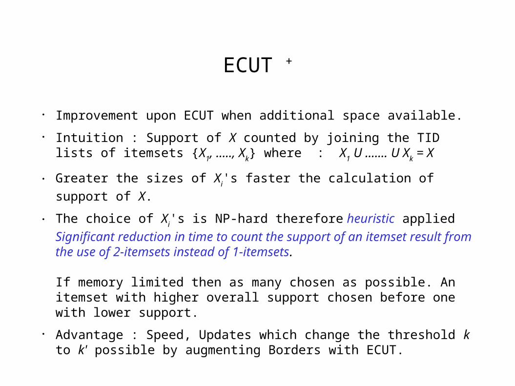
ECUT +

● Improvement upon ECUT when additional space available.

● Intuition : Support of X counted by joining the TID lists of itemsets {X

1, ....., X

k} where : X

1 U ....... U X

k = X

● Greater the sizes of Xi's faster the calculation of support of X.

● The choice of Xi's is NP-hard therefore heuristic applied

Significant reduction in time to count the support of an itemset result from the use of 2-itemsets instead of 1-itemsets.

If memory limited then as many chosen as possible. An itemset with higher overall support chosen before one with lower support.

● Advantage : Speed, Updates which change the threshold k to k' possible by augmenting Borders with ECUT.

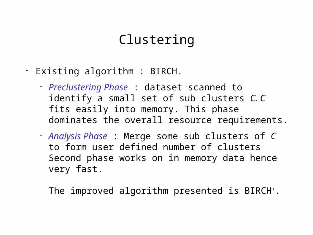
Clustering

● Existing algorithm : BIRCH.

– Preclustering Phase : dataset scanned to identify a small set of sub clusters C. C fits easily into memory. This phase dominates the overall resource requirements.

– Analysis Phase : Merge some sub clusters of C to form user defined number of clusters Second phase works on in memory data hence very fast.

The improved algorithm presented is BIRCH+.

BIRCH+

● Incrementally cluster D[1, t + 1 ] in two steps. Inductive description

– Base case t = 1 run BIRCH on D[ 1 , 1].

– Time t + 1 : output of first phase of BIRCH in memory as set of sub clusters C

t.

– When Dt+1

is added update Ct by scanning D

t+1 as if the first

phase of BIRCH was suspended.

– After obtaining Ct+1

run second phase of BIRCH.

● Observation : Input order of data does not have perceptible impact on quality of clusters produced by BIRCH.

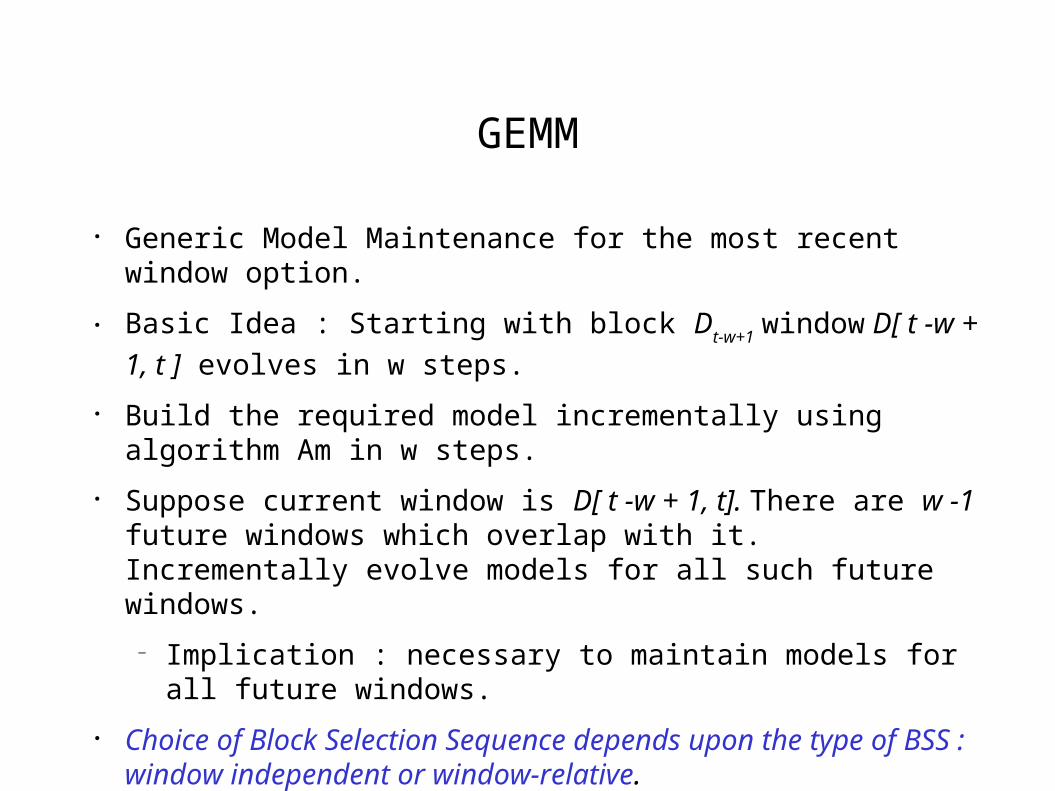
GEMM

● Generic Model Maintenance for the most recent window option.

● Basic Idea : Starting with block Dt-w+1

window D[ t -w + 1, t ]

evolves in w steps.

● Build the required model incrementally using algorithm Am in w steps.

● Suppose current window is D[ t -w + 1, t]. There are w -1 future windows which overlap with it. Incrementally evolve models for all such future windows.

– Implication : necessary to maintain models for all future windows.

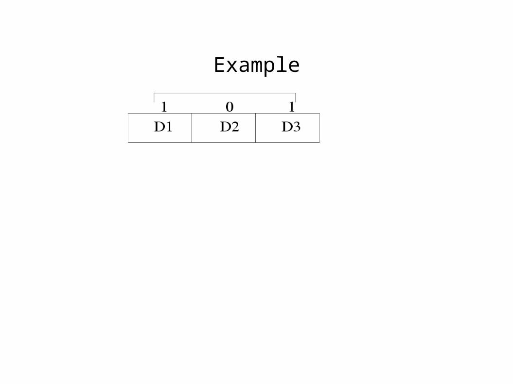
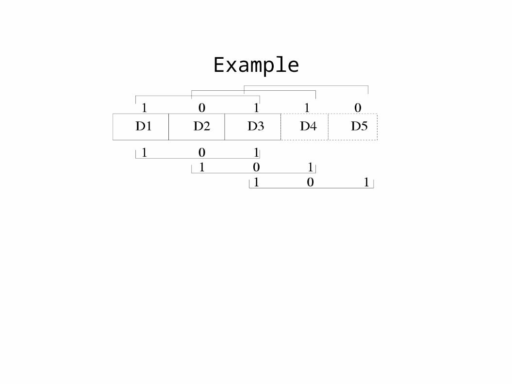
Example

Example

GEMM

● Generic Model Maintenance for the most recent window option.

● Basic Idea : Starting with block Dt-w+1

window D[ t -w + 1, t ]

evolves in w steps.

● Build the required model incrementally using algorithm Am in w steps.

● Suppose current window is D[ t -w + 1, t]. There are w -1 future windows which overlap with it. Incrementally evolve models for all such future windows.

– Implication : necessary to maintain models for all future windows.

● Choice of Block Selection Sequence depends upon the type of BSS : window independent or window-relative.

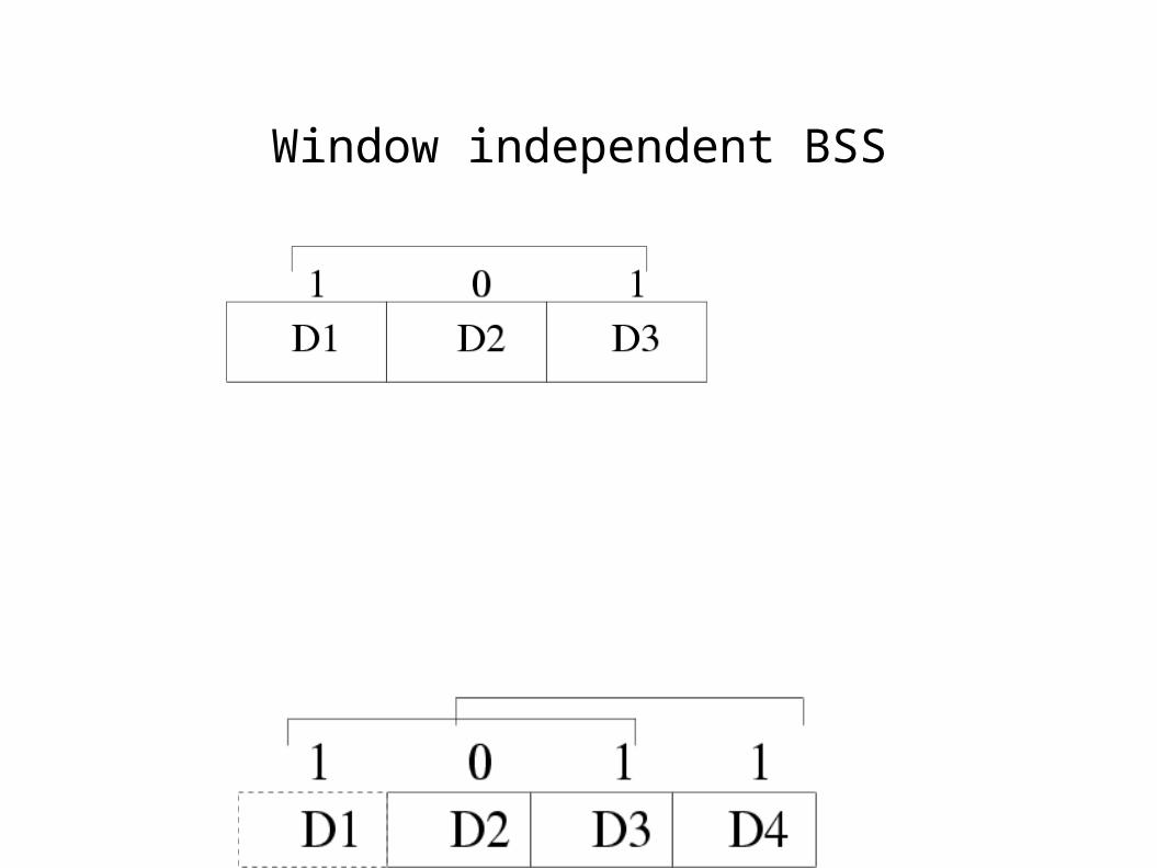
Window independent BSS

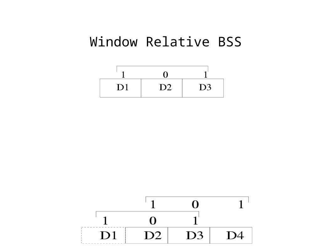
Window Relative BSS

Analysis

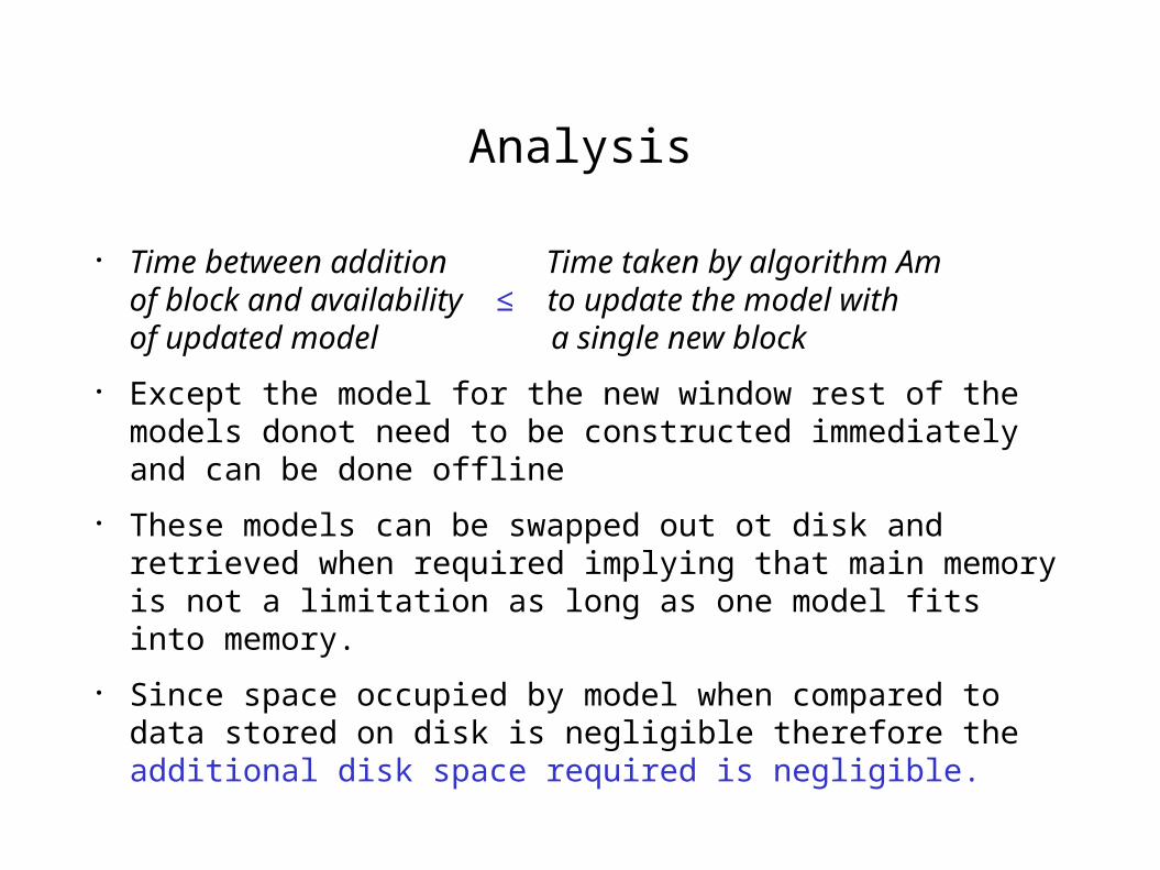
● Time between addition Time taken by algorithm Am of block and availability ≤ to update the model with of updated model a single new block

● Except the model for the new window rest of the models donot need to be constructed immediately and can be done offline

● These models can be swapped out ot disk and retrieved when required implying that main memory is not a limitation as long as one model fits into memory.

● Since space occupied by model when compared to data stored on disk is negligible therefore the additional disk space required is negligible.

Optimizations● Maintenance under deletion of transactions : possible for certain classes of

models for example set of frequent itemsets.

● Algorithm proceeds exactly as for addition of transactions except that support of all itemsets contained in a deleted transaction are decremented.

● Options : a) GEMM with instantiated model maintenance algorithm Am for addition of blocksb) Alternative algorithm that directly updates the model to reflect the addition of new block and deletion of oldest block.

“(b)” maintains a single model whereas GEMM maintains w-1 models. Response time of GEMM is same as time required to add a new block whereas “(b)” has to reflect the addition and deletion. GEMM takes half the time.

● Set of subclusters cannot be maintained under deletion in BIRCH.

● Inefficient to use “(b)” with window relative BSS. For eample BSS <10101010> would cause whole model to be reconstructed in “(b)”.

Performance

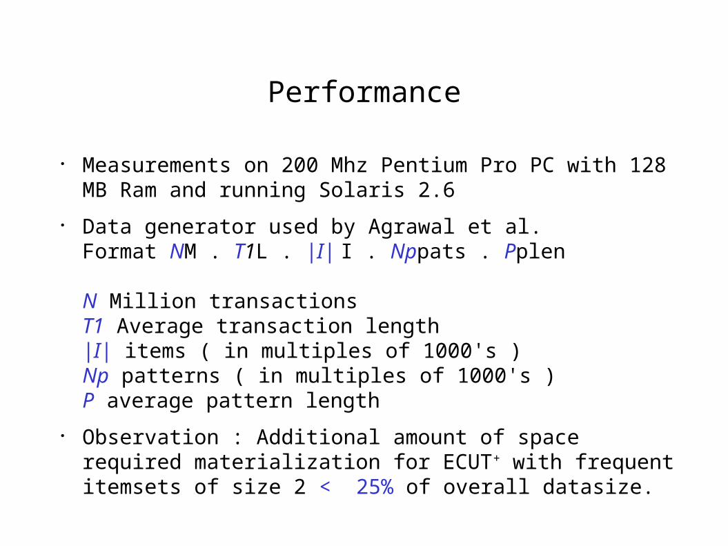
● Measurements on 200 Mhz Pentium Pro PC with 128 MB Ram and running Solaris 2.6

● Data generator used by Agrawal et al. Format NM . T1L . |I| I . Nppats . Pplen

N Million transactionsT1 Average transaction length|I| items ( in multiples of 1000's )Np patterns ( in multiples of 1000's )P average pattern length

● Observation : Additional amount of space required materialization for ECUT+ with frequent itemsets of size 2 < 25% of overall datasize.

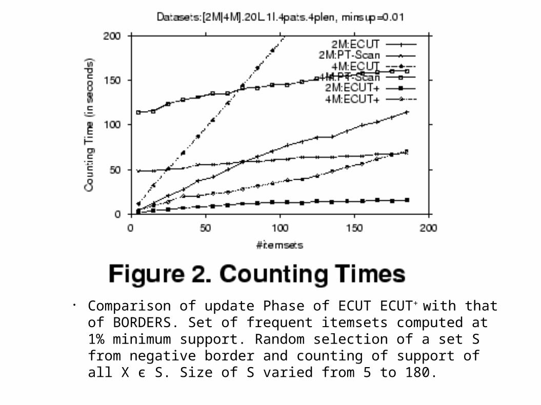
● Comparison of update Phase of ECUT ECUT+ with that of BORDERS. Set of frequent itemsets computed at 1% minimum support. Random selection of a set S from negative border and counting of support of all X є S. Size of S varied from 5 to 180.

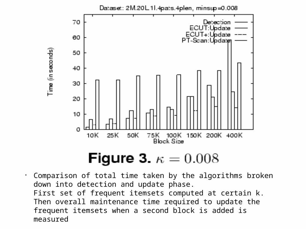
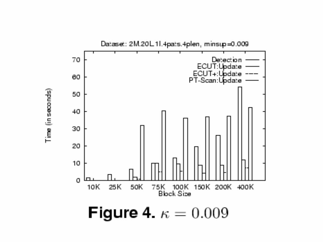
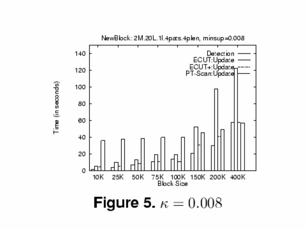
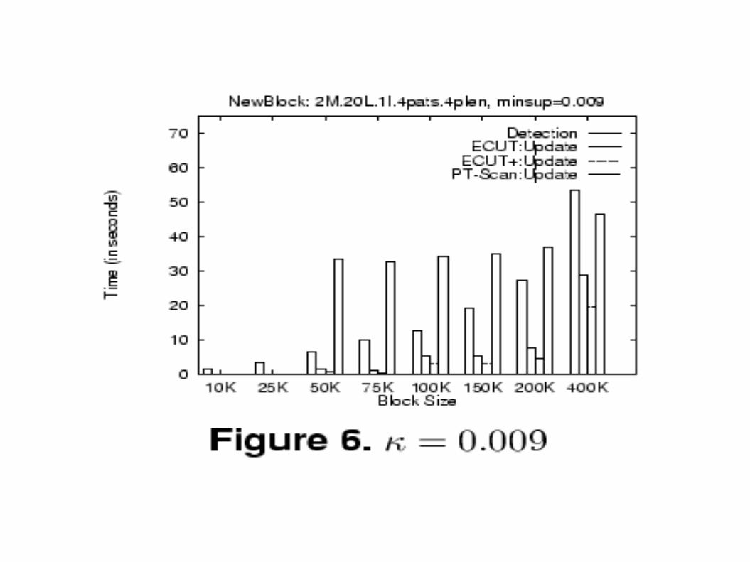
● Comparison of total time taken by the algorithms broken down into detection and update phase. First set of frequent itemsets computed at certain k. Then overall maintenance time required to update the frequent itemsets when a second block is added is measured

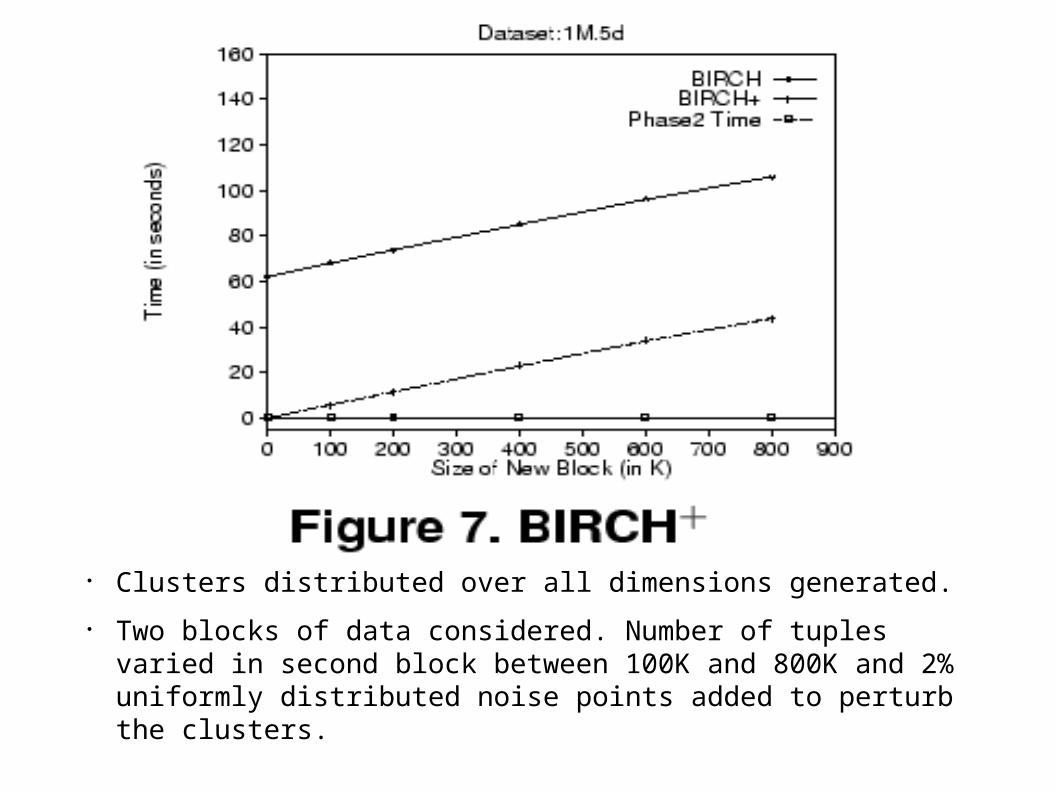
● Clusters distributed over all dimensions generated.

● Two blocks of data considered. Number of tuples varied in second block between 100K and 800K and 2% uniformly distributed noise points added to perturb the clusters.

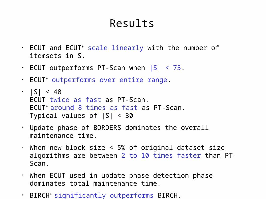
Results

● ECUT and ECUT+ scale linearly with the number of itemsets in S.

● ECUT outperforms PT-Scan when |S| < 75.

● ECUT+ outperforms over entire range.

● |S| < 40ECUT twice as fast as PT-Scan. ECUT+ around 8 times as fast as PT-Scan.Typical values of |S| < 30

● Update phase of BORDERS dominates the overall maintenance time.

● When new block size < 5% of original dataset size algorithms are between 2 to 10 times faster than PT-Scan.

● When ECUT used in update phase detection phase dominates total maintenance time.

● BIRCH+ significantly outperforms BIRCH.

Conclusion

● Problem space of systematic data evolution explored and efficient model-maintenance algorithms presented.

● All the algorithms presented are actually very simple modifications of existing algorithms and seem to be quite effective.