Embed Size (px)
Citation preview

Demystifying deep learningPetar Velickovic
Artificial Intelligence GroupDepartment of Computer Science and Technology, University of Cambridge, UK
London Data Science Summit 20 October 2017
Introduction
I In this talk, I will guide you through a condensed story of howdeep learning became what it was today, and where it’s going.
I This will involve a journey through the essentials of how neuralnetworks normally work, and an overview of some of theirmany variations and applications.
I Not a deep learning tutorial! (wait for Sunday. :))
I Disclaimer: Any views expressed (especially with respect toinfluential papers) are entirely my own, and influenced perhapsby the kinds of problems I’m solving. It’s fairly certain that anydeep learning researcher would give a different account ofwhat’s the most important work in the field. :)
Motivation: notMNIST
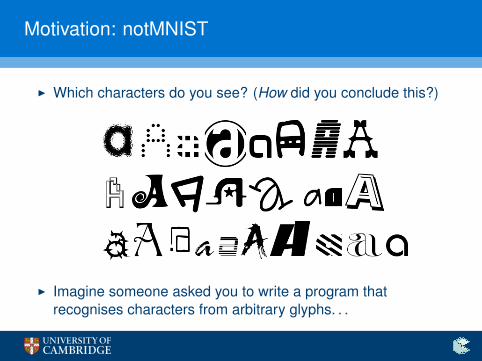
I Which characters do you see? (How did you conclude this?)
I Imagine someone asked you to write a program thatrecognises characters from arbitrary glyphs. . .
Intelligent systems
I Although the previous task was likely simple to you, you(probably) couldn’t turn your thought process into a concisesequence of instructions for a program!
I Unlike a “dumb” program (that just blindly executespreprogrammed instructions), you’ve been exposed to a lot of Acharacters during your lifetimes, and eventually “learnt” thecomplex features making something an A!
I Desire to design such systems (capable of generalising frompast experiences) is the essence of machine learning!
I How many such systems do we know from nature?
Specialisation in the brain
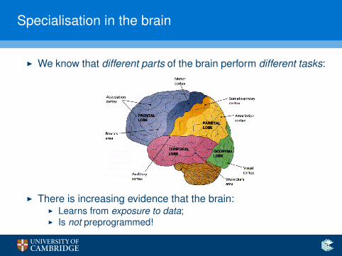
I We know that different parts of the brain perform different tasks:
I There is increasing evidence that the brain:I Learns from exposure to data;I Is not preprogrammed!
Brain & data
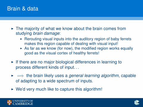
I The majority of what we know about the brain comes fromstudying brain damage:
I Rerouting visual inputs into the auditory region of baby ferretsmakes this region capable of dealing with visual input!
I As far as we know (for now), the modified region works equallygood as the visual cortex of healthy ferrets!
I If there are no major biological differences in learning toprocess different kinds of input. . .
I =⇒ the brain likely uses a general learning algorithm, capableof adapting to a wide spectrum of inputs.
I We’d very much like to capture this algorithm!
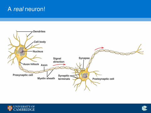
A real neuron!
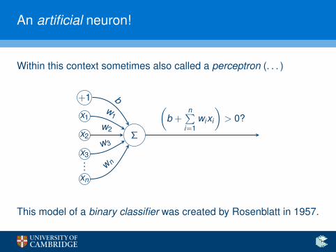
An artificial neuron!
Within this context sometimes also called a perceptron (. . . )
Σ
+1
x1
x2
x3
xn
bw
1
w2
w3
w n(
b +n∑
i=1wixi
)> 0?
...
This model of a binary classifier was created by Rosenblatt in 1957.
Gradient descent
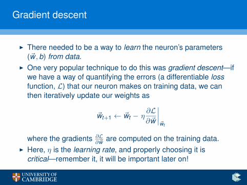
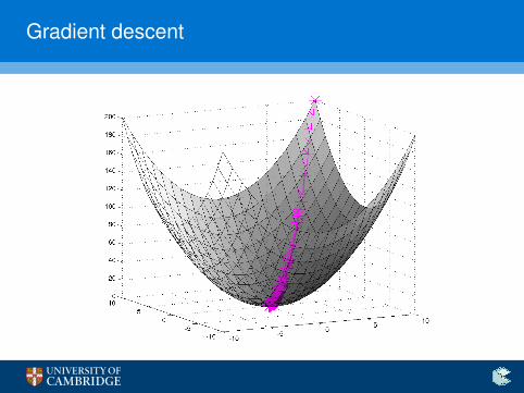
I There needed to be a way to learn the neuron’s parameters(~w ,b) from data.
I One very popular technique to do this was gradient descent—ifwe have a way of quantifying the errors (a differentiable lossfunction, L) that our neuron makes on training data, we canthen iteratively update our weights as
~wt+1 ← ~wt − η∂L∂~w
∣∣∣∣~wt
where the gradients ∂L∂~w are computed on the training data.
I Here, η is the learning rate, and properly choosing it iscritical—remember it, it will be important later on!
Gradient descent
Custom activations
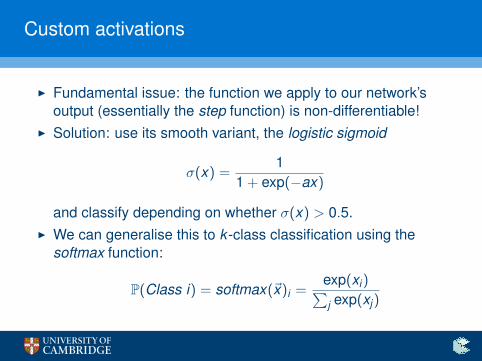
I Fundamental issue: the function we apply to our network’soutput (essentially the step function) is non-differentiable!
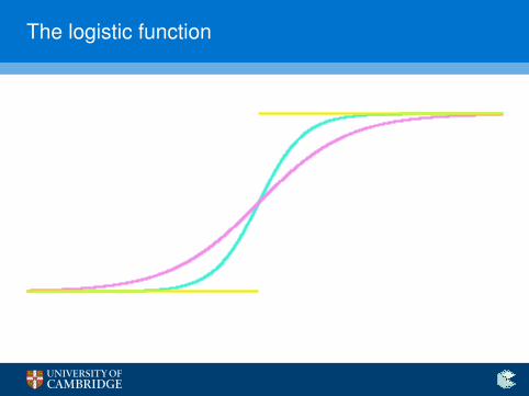
I Solution: use its smooth variant, the logistic sigmoid
σ(x) =1
1 + exp(−ax)
and classify depending on whether σ(x) > 0.5.I We can generalise this to k -class classification using the
softmax function:
P(Class i) = softmax(~x)i =exp(xi)∑j exp(xj)
The logistic function
0
0.5
1
The loss function
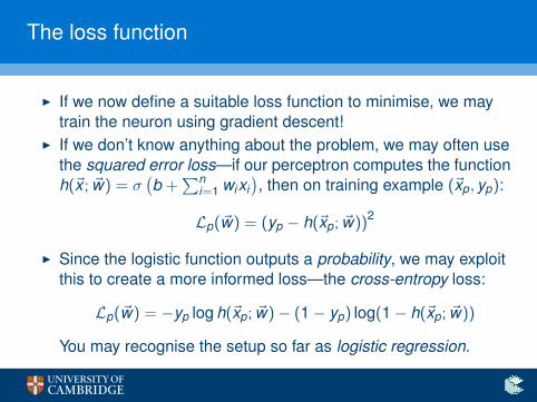
I If we now define a suitable loss function to minimise, we maytrain the neuron using gradient descent!
I If we don’t know anything about the problem, we may often usethe squared error loss—if our perceptron computes the functionh(~x ; ~w) = σ
(b +
∑ni=1 wixi
), then on training example (~xp, yp):
Lp(~w) = (yp − h(~xp; ~w))2
I Since the logistic function outputs a probability, we may exploitthis to create a more informed loss—the cross-entropy loss:
Lp(~w) = −yp log h(~xp; ~w)− (1− yp) log(1− h(~xp; ~w))
You may recognise the setup so far as logistic regression.
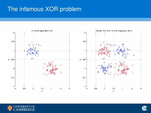
The infamous XOR problem
Neural networks and deep learning
I To get any further, we need to be able to introduce nonlinearityinto the function our system computes.
I It is easy to extend a single neuron to a neural network—simplyconnect outputs of neurons to inputs of other neurons.
I If we apply nonlinear activation functions to intermediateoutputs, this will introduce the desirable properties.
I Typically we organise neural networks in a sequence of layers,such that a single layer only processes output from theprevious layer.
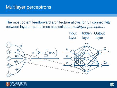
Multilayer perceptrons
The most potent feedforward architecture allows for full connectivitybetween layers—sometimes also called a multilayer perceptron.
Σ σ
+1
x1
x2
x3
xn
bw
1
w2
w3
w n
σ
(b +
n∑i=1
wixi
)
...
I1
I2
I3
Inputlayer
Hiddenlayer
Outputlayer
O1
O2
Backpropagation
I Variants of multilayer perceptrons (MLPs) have been knownsince the 1960s. In a way, everything that modern deeplearning is utilising are specialised MLPs!
I Stacking neurons in this manner will preserve differentiability,so we can re-use gradient descent to train them once again.
I However, computing ∂L∂w ′ for an arbitrary weight w ′ in such a
network was not initially very efficient. . .
I . . . until 1985, when the backpropagation algorithm wasintroduced by Rumelhart, Hinton and Williams.
Backpropagation
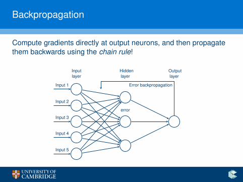
Compute gradients directly at output neurons, and then propagatethem backwards using the chain rule!
Inputlayer
Hiddenlayer
Outputlayer
Input 1
Input 2
Input 3
Input 4
Input 5
error
Error backpropagation

Hyperparameters
I Gradient descent optimises solely the weights and biases inthe network. How about:
I the number of hidden layers?I the amount of neurons in each hidden layer?I the activation functions of these neurons?I the number of iterations of gradient descent?I the learning rate?I . . .
I These parameters must be fixed before training commences!For this reason, we often call them hyperparameters.
I Optimising them remains an extremely difficult problem—weoften can’t do better than separating some of our training datafor evaluating various combinations of hyperparameter values.
Neural network depth
I I’d like to highlight a specific hyperparameter: the number ofhidden layers, i.e. the network’s depth.
I What do you think, how many hidden layers are sufficient tolearn any (bounded continuous) real function?
I One! (Cybenko’s theorem, 1989.)
I However, the proof is not constructive, i.e. does not give theoptimal width of this layer or a training algorithm.
I We must go deeper. . .I Every network with > 1 hidden layer is considered deep!I Today’s state-of-the-art networks often have over 150 layers.
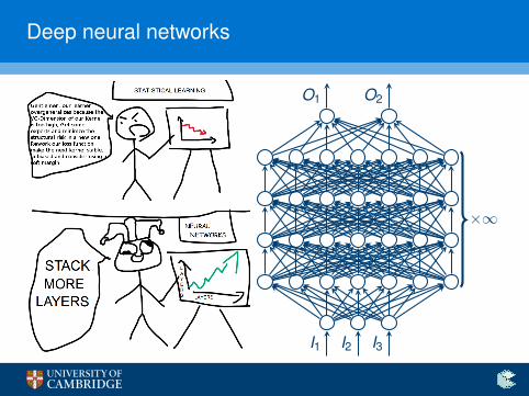
Deep neural networks
I3I2I1
O2O1
×∞
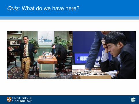
Quiz: What do we have here?
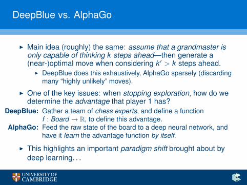
DeepBlue vs. AlphaGo
I Main idea (roughly) the same: assume that a grandmaster isonly capable of thinking k steps ahead—then generate a(near-)optimal move when considering k ′ > k steps ahead.
I DeepBlue does this exhaustively, AlphaGo sparsely (discardingmany “highly unlikely” moves).
I One of the key issues: when stopping exploration, how do wedetermine the advantage that player 1 has?
DeepBlue: Gather a team of chess experts, and define a functionf : Board → R, to define this advantage.
AlphaGo: Feed the raw state of the board to a deep neural network, andhave it learn the advantage function by itself.
I This highlights an important paradigm shift brought about bydeep learning. . .
Feature engineering
I Historically, machine learning problems were tackled bydefining a set of features to be manually extracted from rawdata, and given as inputs for “shallow” models.
I Many scientists built entire PhDs focusing on features of interestfor just one such problem!
I Generalisability: very small (often zero)!
I With deep learning, the network learns the best features byitself, directly from raw data!
I For the first time connected researchers from fully distinct areas,e.g. natural language processing and computer vision.
I =⇒ a person capable of working with deep neural networksmay readily apply their knowledge to create state-of-the-artmodels in virtually any domain (assuming a large dataset)!
Representation learning
I As inputs propagate through the layers, the network capturesmore complex representations of them.
I It will be extremely valuable for us to be able to reason aboutthese representations!
I Typically, models that deal with images will tend to have thebest visualisations.
I Therefore, I will now provide a brief introduction to thesemodels (convolutional neural networks). Then we can look intothe kinds of representations they capture. . .
Working with images
I Simple fully-connected neural networks (as described already)typically fail on high-dimensional datasets (e.g. images).
I Treating each pixel as an independent input. . .I . . . results in h × w × d new parameters per neuron in the first
hidden layer. . .I . . . quickly deteriorating as images become larger—requiring
exponentially more data to properly fit those parameters!
I Key idea: downsample the image until it is small enough to betackled by such a network!
I Would ideally want to extract some useful features first. . .
I =⇒ exploit spatial structure!
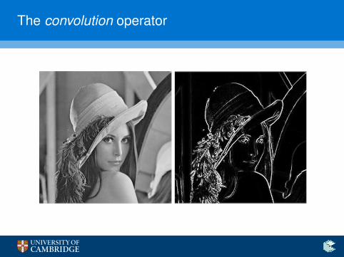
The convolution operator
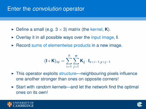
Enter the convolution operator
I Define a small (e.g. 3× 3) matrix (the kernel, K).
I Overlay it in all possible ways over the input image, I.
I Record sums of elementwise products in a new image.
(I ∗ K)xy =h∑
i=1
w∑j=1
Kij · Ix+i−1,y+j−1
I This operator exploits structure—neighbouring pixels influenceone another stronger than ones on opposite corners!
I Start with random kernels—and let the network find the optimalones on its own!
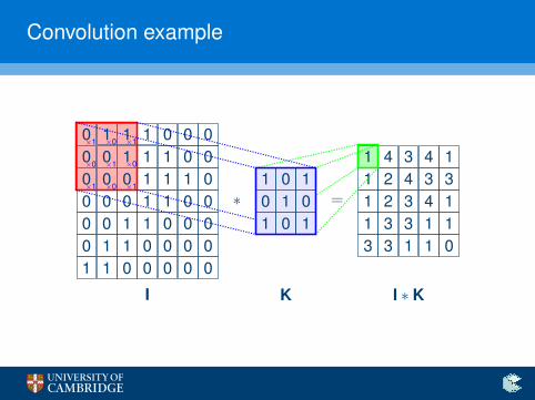
Convolution example
0 1 1 1 0 0 00 0 1 1 1 0 00 0 0 1 1 1 00 0 0 1 1 0 00 0 1 1 0 0 00 1 1 0 0 0 01 1 0 0 0 0 0
I
∗1 0 10 1 01 0 1
K
=
1 4 3 4 11 2 4 3 31 2 3 4 11 3 3 1 13 3 1 1 0
I ∗ K
1 0 10 1 01 0 1
×1 ×0 ×1
×0 ×1 ×0
×1 ×0 ×1
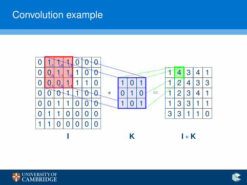
Convolution example
0 1 1 1 0 0 00 0 1 1 1 0 00 0 0 1 1 1 00 0 0 1 1 0 00 0 1 1 0 0 00 1 1 0 0 0 01 1 0 0 0 0 0
I
∗1 0 10 1 01 0 1
K
=
1 4 3 4 11 2 4 3 31 2 3 4 11 3 3 1 13 3 1 1 0
I ∗ K
1 0 10 1 01 0 1
×1 ×0 ×1
×0 ×1 ×0
×1 ×0 ×1
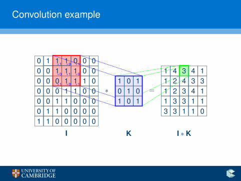
Convolution example
0 1 1 1 0 0 00 0 1 1 1 0 00 0 0 1 1 1 00 0 0 1 1 0 00 0 1 1 0 0 00 1 1 0 0 0 01 1 0 0 0 0 0
I
∗1 0 10 1 01 0 1
K
=
1 4 3 4 11 2 4 3 31 2 3 4 11 3 3 1 13 3 1 1 0
I ∗ K
1 0 10 1 01 0 1
×1 ×0 ×1
×0 ×1 ×0
×1 ×0 ×1
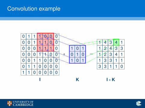
Convolution example
0 1 1 1 0 0 00 0 1 1 1 0 00 0 0 1 1 1 00 0 0 1 1 0 00 0 1 1 0 0 00 1 1 0 0 0 01 1 0 0 0 0 0
I
∗1 0 10 1 01 0 1
K
=
1 4 3 4 11 2 4 3 31 2 3 4 11 3 3 1 13 3 1 1 0
I ∗ K
1 0 10 1 01 0 1
×1 ×0 ×1
×0 ×1 ×0
×1 ×0 ×1
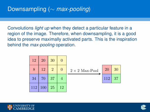
Downsampling (∼ max-pooling)
Convolutions light up when they detect a particular feature in aregion of the image. Therefore, when downsampling, it is a goodidea to preserve maximally activated parts. This is the inspirationbehind the max-pooling operation.
12 20 30 0
8 12 2 0
34 70 37 4
112 100 25 12
20 30
112 37
2× 2 Max-Pool
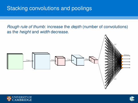
Stacking convolutions and poolings
Rough rule of thumb: increase the depth (number of convolutions)as the height and width decrease.
Conv. Pool Conv. Pool
FC
FC
Softmax
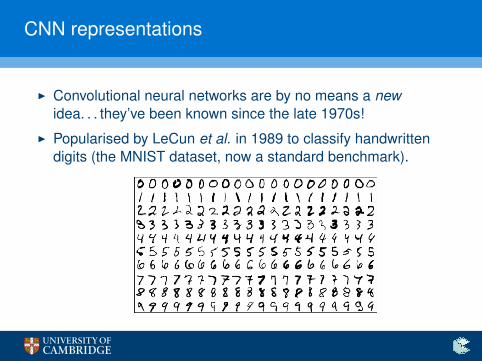
CNN representations
I Convolutional neural networks are by no means a newidea. . . they’ve been known since the late 1970s!
I Popularised by LeCun et al. in 1989 to classify handwrittendigits (the MNIST dataset, now a standard benchmark).
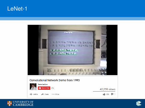
LeNet-1
Observing kernels
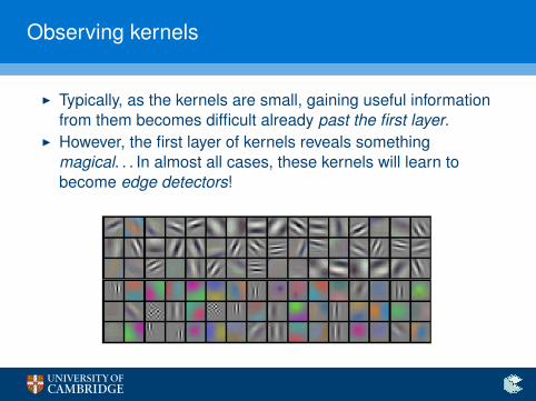
I Typically, as the kernels are small, gaining useful informationfrom them becomes difficult already past the first layer.
I However, the first layer of kernels reveals somethingmagical. . . In almost all cases, these kernels will learn tobecome edge detectors!
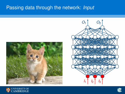
Passing data through the network: Input
I3I2I1
O2O1
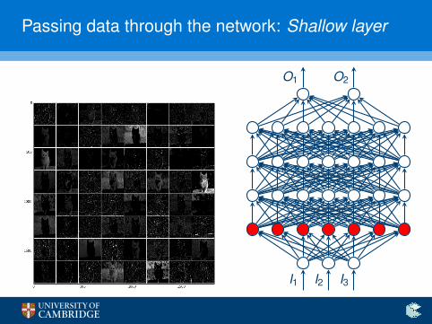
Passing data through the network: Shallow layer
I3I2I1
O2O1

Passing data through the network: Deep layer
I3I2I1
O2O1
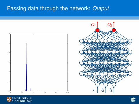
Passing data through the network: Output
I3I2I1
O2O1
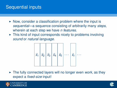
Sequential inputs
I Now, consider a classification problem where the input issequential—a sequence consisting of arbitrarily many steps,wherein at each step we have n features.
I This kind of input corresponds nicely to problems involvingsound or natural language.
~x1 ~x2 ~x3 ~x4 ~x5 . . . ~xt . . .
I The fully connected layers will no longer even work, as theyexpect a fixed-size input!
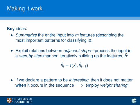
Making it work
Key ideas:I Summarize the entire input into m features (describing the
most important patterns for classifying it);
I Exploit relations between adjacent steps—process the input ina step-by-step manner, iteratively building up the features, ~h:
~ht = f (~xt , ~ht−1)
I If we declare a pattern to be interesting, then it does not matterwhen it occurs in the sequence =⇒ employ weight sharing!
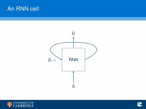
An RNN cell
RNN
~xt
~yt
~yt−1
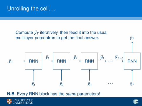
Unrolling the cell. . .
RNN RNN RNN
Compute ~yT iteratively, then feed it into the usualmultilayer perceptron to get the final answer.
. . . RNN
~x1 ~x2 ~x3 ~xT
~yT
~y0
~y1 ~y2 ~y3 ~yT−1
. . .
N.B. Every RNN block has the same parameters!
RNN variants
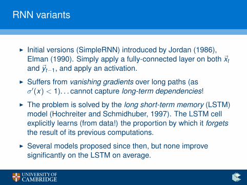
I Initial versions (SimpleRNN) introduced by Jordan (1986),Elman (1990). Simply apply a fully-connected layer on both ~xtand ~yt−1, and apply an activation.
I Suffers from vanishing gradients over long paths (asσ′(x) < 1). . . cannot capture long-term dependencies!
I The problem is solved by the long short-term memory (LSTM)model (Hochreiter and Schmidhuber, 1997). The LSTM cellexplicitly learns (from data!) the proportion by which it forgetsthe result of its previous computations.
I Several models proposed since then, but none improvesignificantly on the LSTM on average.
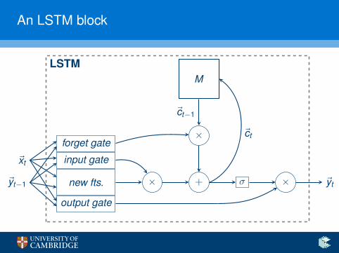
An LSTM block
new fts.
input gate
forget gate
output gate
~xt
~yt−1 × + σ × ~yt
×
M
~ct−1
~ct
LSTM
Where are we?
I By now, we’ve covered all the essential architectures that areused across the board for modern deep learning. . .
I . . . and we’re not even in the 21st century yet!
I It turns out that we had the required methodology all along, butseveral key factors were missing. . .
I demanding gamers (∼ GPU development!)I
:::::::::::::big companies (∼ lots of resources, and DL frameworks!)
I big data (∼ for big parameter spaces!)
I So, what’s exactly new, methodologically?
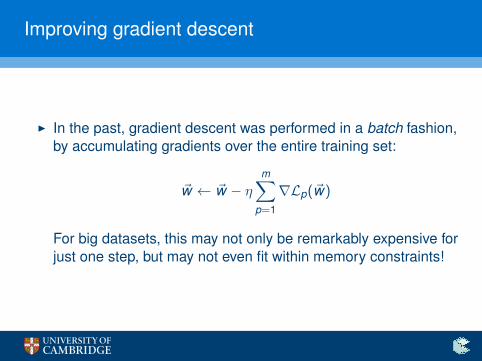
Improving gradient descent
I In the past, gradient descent was performed in a batch fashion,by accumulating gradients over the entire training set:
~w ← ~w − ηm∑
p=1
∇Lp(~w)
For big datasets, this may not only be remarkably expensive forjust one step, but may not even fit within memory constraints!
Stochastic gradient descent (SGD)
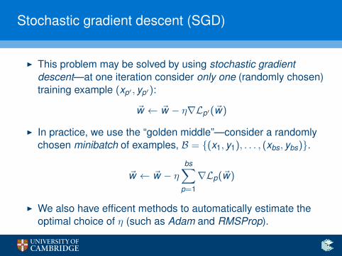
I This problem may be solved by using stochastic gradientdescent—at one iteration consider only one (randomly chosen)training example (xp′ , yp′):
~w ← ~w − η∇Lp′(~w)
I In practice, we use the “golden middle”—consider a randomlychosen minibatch of examples, B = {(x1, y1), . . . , (xbs, ybs)}.
~w ← ~w − ηbs∑
p=1
∇Lp(~w)
I We also have efficent methods to automatically estimate theoptimal choice of η (such as Adam and RMSProp).
Vanishing gradients strike back
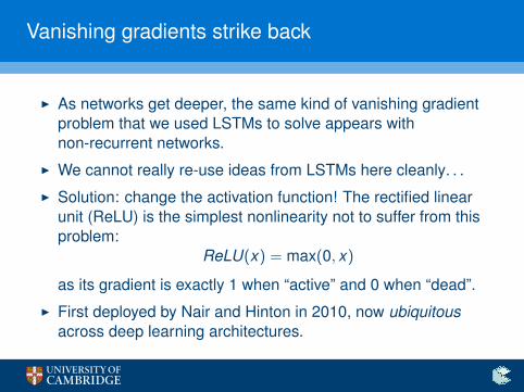
I As networks get deeper, the same kind of vanishing gradientproblem that we used LSTMs to solve appears withnon-recurrent networks.
I We cannot really re-use ideas from LSTMs here cleanly. . .
I Solution: change the activation function! The rectified linearunit (ReLU) is the simplest nonlinearity not to suffer from thisproblem:
ReLU(x) = max(0, x)
as its gradient is exactly 1 when “active” and 0 when “dead”.
I First deployed by Nair and Hinton in 2010, now ubiquitousacross deep learning architectures.
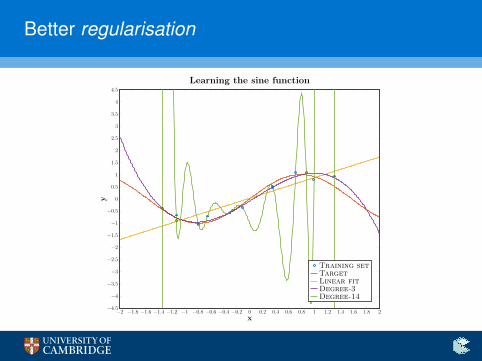
Better regularisation
−2 −1.8 −1.6 −1.4 −1.2 −1 −0.8 −0.6 −0.4 −0.2 0 0.2 0.4 0.6 0.8 1 1.2 1.4 1.6 1.8 2−4.5
−4
−3.5
−3
−2.5
−2
−1.5
−1
−0.5
0
0.5
1
1.5
2
2.5
3
3.5
4
4.5
x
y
Learning the sine function
Training setTargetLinear fitDegree-3Degree-14
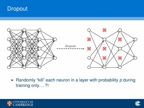
Dropout
dropout ××
×
×
×
×
×
I Randomly “kill” each neuron in a layer with probability p duringtraining only. . . ?!
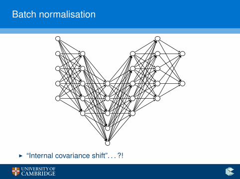
Batch normalisation
I “Internal covariance shift”. . . ?!
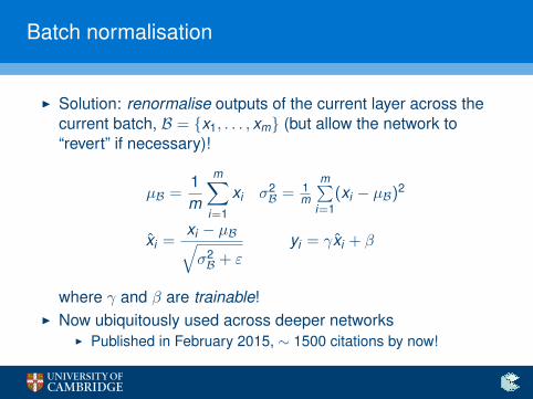
Batch normalisation
I Solution: renormalise outputs of the current layer across thecurrent batch, B = {x1, . . . , xm} (but allow the network to“revert” if necessary)!
µB =1m
m∑i=1
xi σ2B = 1
m
m∑i=1
(xi − µB)2
xi =xi − µB√σ2B + ε
yi = γxi + β
where γ and β are trainable!I Now ubiquitously used across deeper networks
I Published in February 2015, ∼ 1500 citations by now!
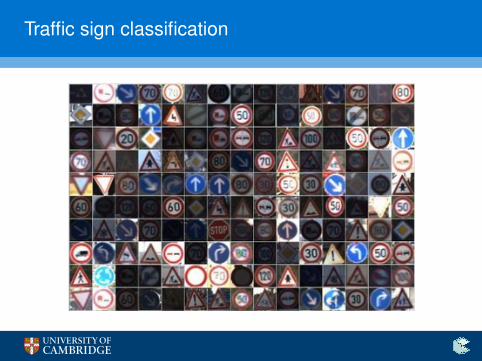
Traffic sign classification
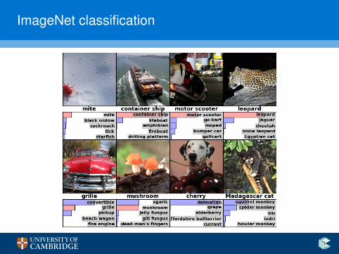
ImageNet classification
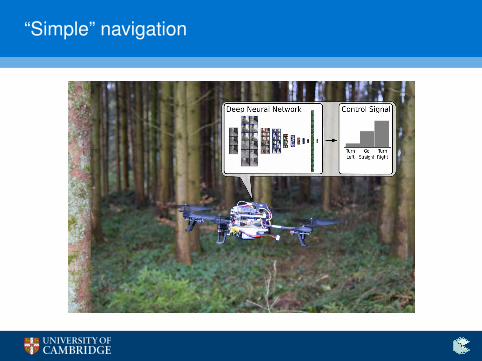
“Simple” navigation
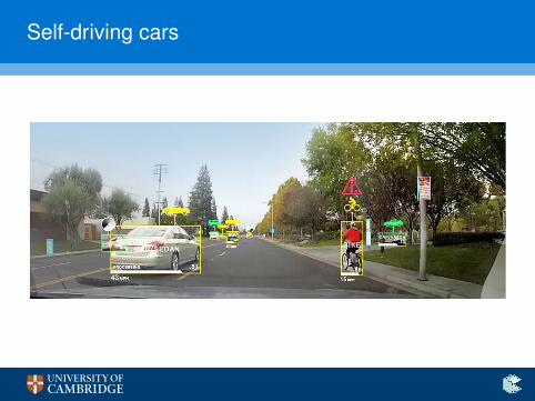
Self-driving cars

“Greatest hits”
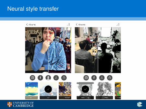
Neural style transfer
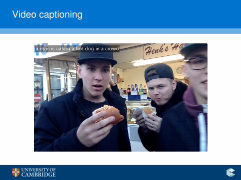
Video captioning
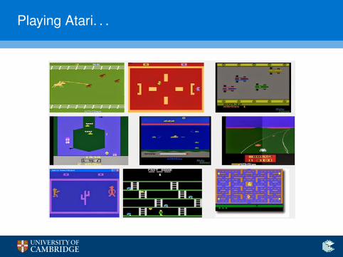
Playing Atari. . .
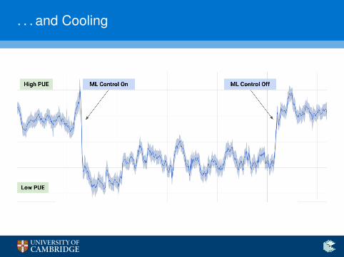
. . . and Cooling
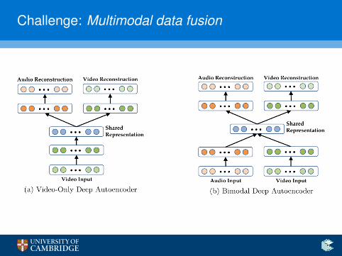
Challenge: Multimodal data fusion
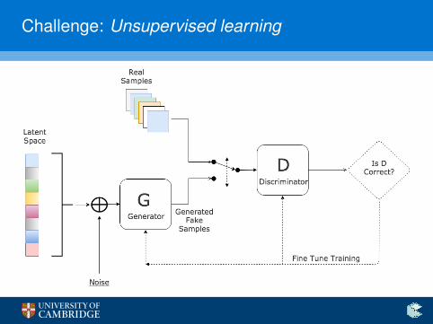
Challenge: Unsupervised learning
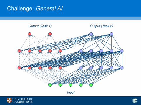
Challenge: General AI
Input
Output (Task 1) Output (Task 2)