Density Functional Theory for Beginners

Basic Principles and Practical Approaches

Fabio Finocchi

Institut des NanoSciences de Paris (INSP)CNRS and University Pierre et Marie Curie

October 24, 2011

1To the memory of Elena, who made me feel any small progress along the completion of thesenotes extremely important.

Contents

1 Introduction 2

2 Basic DFT theory 52.1 Why is the problem difficult . . . . . . . . . . . . . . . . . . . . . . . . . . . . . . . . . . . 5

2.1.1 Functionals . . . . . . . . . . . . . . . . . . . . . . . . . . . . . . . . . . . . . . . . 62.2 Electron density as the basic variable . . . . . . . . . . . . . . . . . . . . . . . . . . . . . . 72.3 Towards the definition of the energy functional . . . . . . . . . . . . . . . . . . . . . . . . 92.4 Finding the ground state: total energy and electron density . . . . . . . . . . . . . . . . . 11

2.4.1 Minimizing E[n] . . . . . . . . . . . . . . . . . . . . . . . . . . . . . . . . . . . . . 112.4.2 The Kohn-Sham equations . . . . . . . . . . . . . . . . . . . . . . . . . . . . . . . 132.4.3 Computing the total energy . . . . . . . . . . . . . . . . . . . . . . . . . . . . . . . 15

2.5 The Exchange-Correlation energy functional . . . . . . . . . . . . . . . . . . . . . . . . . . 16

3 Practical Implementation 203.1 Solving the Kohn-Sham equations: basis sets . . . . . . . . . . . . . . . . . . . . . . . . . 20

3.1.1 Pseudo-potentials . . . . . . . . . . . . . . . . . . . . . . . . . . . . . . . . . . . . . 223.1.2 Plane waves . . . . . . . . . . . . . . . . . . . . . . . . . . . . . . . . . . . . . . . . 23

3.2 Solving the Kohn-Sham equations: the self-consistent cycle . . . . . . . . . . . . . . . . . 30

4 Density Functional Perturbation Theory 344.1 The basic formalism. . . . . . . . . . . . . . . . . . . . . . . . . . . . . . . . . . . . . . . . 344.2 First-order energy derivatives and atomic forces. . . . . . . . . . . . . . . . . . . . . . . . 354.3 Second order . . . . . . . . . . . . . . . . . . . . . . . . . . . . . . . . . . . . . . . . . . . 38

1

Chapter 1

Introduction

Numerical Simulations and Materials Science Physicists have a talent for producing equationsthat they are quite unable to solve. This is likely the basic reason why numerical simulations havebecome ubiquitous in most fields of physics, including materials science, condensed matter physics andnano-sciences. Experiments can often be difficult to carry out, expensive and sometimes provide onlyindirect information. For instance, X-ray diffraction must be complemented by appropriate computerprograms in order to find out atomic positions in a complex crystal. Moreover, X-ray diffraction canidentify where atoms are, not why the actual structure is preferred to another one. The interpretationof the experimental data often requires hypothesis or models that should be validated independently.Numerical simulations can provide a valuable help to explain the experimental data on the basis of amicroscopic model and give insights into the basic mechanisms of interaction between atoms. Simulationscan also be useful to obtain the numerical solution of equations that cannot be solved by analytical means,and provide benchmarks for approximated theories or simplified models.

The standard use of numerical simulations is ultimately due to the fast improvements of the computerpower and the development of new and more and more effective numerical methods. As far as materialsscience is concerned, some important dates must be recalled.

1. The invention of the first device that resembles modern computers in the 40’s;

2. N. Metropolis proposed a new algorithm, based on the Monte Carlo method, (1) to sample astatistical distribution (2). It is worth noting, in this respect, that these methods benefited fromalgorithm for generating pseudo-random numbers and the fast development of computing power;

3. In 1959, B.J. Alder and T.E. Wainwright proposed a way to integrate the equations of motion forN particles numerically (3). This is the beginning of Molecular Dynamics simulations.

4. In 1985, R. Car and M. Parrinello designed a unified approach for Molecular Dynamics and first-principle calculations within the Density Functional Theory (4). Their work opened a way tosimulate the dynamics of condensed matter systems for which semi-empirical interatomic potentialsare inappropriate.

Ab initio methods In order to investigate systems at the nanoscale, it is necessary to model theinteractions between atoms as accurately as possible, while ensuring that the calculations remain compu-tationally feasible. Often, empirical interatomic potentials, which are usually fitted in order to reproducesome measured physical properties, are adopted. A well known example is provided by Lennard-Jones

potentials, of the form: V (r) = 4ε[σ12

r12 −σ6

r6

], where r is the interatomic distance and ε and σ two

adjustable parameters. The Lennard-Jones potential is well suited to the simulation of van der Waalsinteractions. However, the chemical bond in strongly covalent systems, such as Carbon or Silicon, cannotbe simulated by LJ potentials. Interatomic potentials are limited by the accuracy of the parametrisation,and correspondingly, their transferability to different environments or their ability to reproduce physicalproperties, other than those which they were designed for, can be poor. Indeed, the interaction betweenatoms does depend on their neighbors and, more generally, on their environment. For instance, surfaceatoms experience a different electrostatic field (generally weaker) and have a reduced number of neighbors

2

than atoms in the bulk. For example, bulk-derived potentials may fail in describing molecules, surfaces orsystems at the nanoscale, where the atomic environment strongly differ from that in the perfect crystal.

Furthermore, the type of bonding ultimately depends on the electronic structure of the material, whichis affected by its short and long range order. The interplay between the electronic and structural degrees offreedom (atomic positions and coordination number, space group if any, medium range order in disorderedor polycrystalline materials, etc.) is well documented in materials science. Usually, interatomic potentialsare fitted to a particular system or to a class of materials, with implicit assumptions regarding the type ofbonding. Systems showing a chemical complexity (i.e. crystals with several chemical species, or disorderedmaterials with many inequivalent impurities) are rather difficult to be treated by interatomic potentials.A large number of distinct bonds should be accounted for, which could be done by introducing manyadjustable parameters in the potential, at the expense of reducing its simplicity and raising the problemof testing its reliability in a large number of cases. Even for elemental systems, interatomic potentialsmay be inappropriate, as documented by the case of a very important material such as Si. Most availableinteratomic potentials for Si are indeed fitted to its diamond structure, which is semiconducting, withSi atoms in the characteristic tetrahedral coordination. All of them provide a bad description of theliquid state, which is metallic with Si atoms having a coordination number close to 6. Another exampleis bond breaking or bond formation during chemical reactions, which are usually accompanied by theredistribution of valence electrons.

Last but not least, all the electronic properties of materials are out of reach of interatomic potentials,which do not account explicitly for the electronic structure. Nowadays, several techniques probe theelectronic rather than the atomic structure. This is the case of Scanning Tunneling Microscopy, photonand electron spectroscopies and other experimental methods. For all these reasons, theoretical approachesthat give access to the electronic structure are highly desirable in the field of nano- and materials sciences.

Modelling interactions with no a priori knowledge of the bonding requires the use of sophisticatedmethodologies, in which one attempts to solve the Schrdinger equation for the electrons. All the methodsthat are based upon the determination of the bonding starting from the basic theorems of quantummechanics are called ab initio (or first-principles) methods. They are not necessarily exact, since someapproximations are generally made at some stage of the theory or of its practical implementation, in orderto make calculations feasible. However, first-principles approaches make no use of experimental inputand, although quite computationally intensive, they have the advantage of being completely transferable,requiring only the atomic constituents of the system under consideration to be specified. Ab initiomethods are thus more intellectually appealing; moreover, they may be used to calculate the propertiesof systems about which no a priori knowledge exists, that is, they are predictive. As a consequence,they can be used as effective methods to study the properties of materials, interpret the experiments,check the accuracy of simpler simulation schemes or even parametrise classical potentials allowing thecomputational restrictions associated with ab initio methods to be circumvented. It is for these reasonsthat ab initio approaches are widely and often routinely used nowadays in the simulation of materials.An example are infrared spectra, which yield the characteristic vibrational frequencies of a material, butgive no insights on the nature of the vibrational modes unless reference spectra are available. Infraredspectra can now be interpreted through ab initio simulations (see chapter 4).

However, the straightforward resolution of the Schrodinger equation HΨ = EΨ for many-electronsystems is actually impossible (see 2.1). Therefore, approximated methods, such as Hartree-Fock theoryand variational Monte Carlo approaches, have been implemented. Among ab initio methods, the densityfunctional theory (DFT) has become the most popular one. The number of works about the implemen-tation of DFT or using the DFT as a computational scheme is continuously increasing. DFT has becomequite a standard approach, which accompanies and complements other laboratory techniques for studyingmaterials. It seems therefore highly desirable for any materials scientist to know the basics of the theory,its practical implementation in the available codes, as well as its capabilities and shortcomings.

About this book Although many very good books on the DFT are available, most of them address aparticular audience, which, very schematically, is made of graduate students who are willing to acquirea solid background in DFT in order to use it as a tool in material science and active researchers in thefield of computational or theoretical physics and chemistry. All of these people must devote time to godeeply through the theory or to use DFT-based computational schemes for the calculation of materialsproperties. This is not the case of students at the Master level: in a limited amount of time, they have to

3

learn the fundamentals of DFT and go through short hands-on-computer sessions; they cannot generallydispose of a scientific environment that makes them aware of the main shortcomings and difficulties inthe use (and abuse) of the DFT as a computational tool.

Having taught for some years a short course at the Master level on the DFT and its applications inMaterial Science, I am aware of the students’ insatisfaction with the existing books or reviews. Previously,students were also provided with short notes, in the form of slides with extended text that I personallywrote. The former ones were thought of as too difficult, dense or long; the latter ones were generallyfelt as too schematic and not providing complementary matter, such as exercises, questions, extensivebibliography. Therefore, this book is specially conceived for them and aim at filling the lack of a simpleand ready-to-use reference on the DFT and its use to compute materials properties. I do not go deeplyinto the theory and treat only the basic theorems that are at the foundations of DFT. More than formalproofs, I provide some simple exercises or illustrative examples, often taken from other physical problems.Such complementary material is an important part of the book, although formally distinguished fromthe main text. I mention some of the most recent advances in the field of DFT, without aiming atdiscussing them thoroughly. Unavoidably, I made use of my personal opinion and experience in order toselect topics, give an advice about the shortcomings of a particular approach and suggest possible furtherreflexions to the reader. I apologise for any lack of citations or for having skipped relevant subjects; myscope is not to cover the entire DFT but to introduce the reader to the theory as quickly and simply aspossible and, possibly, encourage her/him to read review articles or books on the subject. Sometimes,I summarize the main messages in each chapter, thus helping the reader to review the related concepts.The reader is highly advised to check her/his knowledge by reviewing the exercises that are proposed inthe text.

4

Chapter 2

Basic DFT theory

2.1 Why is the problem difficult

Let’s consider as a simple example benzene (C6H6), which is a rather common molecule, experimentallywell known. C6H6 has N = 42 electrons in total. The many-electron wavefunction Ψ(~r1, σ1; . . . . . . ~rN , σN )1 is a complex scalar field. Its spatial part, which depends on the 3N electron coordinates, is defined ina cartesian space of dimension 3N = 126. Let’s suppose we choose a discrete mesh to represent the wavefunction in space. The diameter of the benzene molecule is about 4.5 A; we take a cubic box 10 A wide,in which the occupied electronic states of the molecule are well localized. We also take M = 50 points tointerpolate the wave function on each spatial coordinate, resulting in a mesh with points that are 0.2 Adistant from each other. Therefore, the determination of any matrix element in the real space requiresM3N = 50126 operations. In order to know the ground state wave function, by using the variationalprinciple, one has to minimize the matrix element 〈ΨHΨ〉/〈ΨΨ〉, where H is the Hamiltonian. Thisrequires a repetition of 50126 operations, several times. For the time being, the most powerful computerscan carry out about 1018 operations per second. Therefore, it is clear that it is impossible to find eventhe ground-state wavefunction of benzene by such a straightforward method (not to even mention theexcited states), since this would require more than a human lifetime.

A solution to such a problem was proposed by Hartree and Fock (see, e.g., the book by Ashcroftand Mermin), who made a simplified assumption about the wavefunction; Ψ is written as a N × Ndeterminant of N one-particle orbitals: Ψ = Det(φ1, . . . , φN ). Then, the energy of the N -electron systemis minimized giving the determinantal form of the wavefunction and a system of N equations for theone-particle orbitals 〈φi〉 is derived. The potential term Vi for the i-th orbital φi depends on the other φj(j 6= i). Vi is usually called the self-consistent field, which means that it has to be found consistently withthe wavefunction Det(φ1, . . . , φN ). From mathematical point of view, the Hartree-Fock equations areintegro-differential equations, thus more involved to be solved than a Schrodinger equations with a fixed

external potential of the type[−~2∇2

2m + V (~r)]φ(~r) = εφ(~r). Nevertheless, the many-electron problem

can be treated in the framework of the Hartree-Fock method, which is implemented in several scientificpackages. This is mainly due to the fact that, instead of dealing with the Schrodinger equation of thetrue N -electron wavefunction, the Hartree-Fock theory allows to solve N coupled one-electron equations,which is a much easier task from the computational point of view.

A basic idea to simplify the N -electron problem consists in finding some physical quantity thatdefines the system uniquely without growing in complexity as a function of the number of electrons N .Obviously, this cannot be the N -electron wavefunction, as shown before. A step further was done inthe sixties with the introduction of the DFT (5; 6), which focuses on the electron density rather thanon the wavefunction. We will see that the current implementations of the DFT are also based on aset of self-consistent equations, namely the Kohn-Sham equations, which are analogous in spirit to theHartree-Fock equations.

1~rj and σj are the spatial and spin coordinate relative to the jth electron, respectively. The wavefunction must obeythe Pauli principle, that is, it must be anti-symmetric when two electrons are exchanged.

5

2.1.1 Functionals

Before going further, let’s briefly recall what a functional is and give some basic rules to compute func-tional derivatives. A functional is traditionally a map from a vector space to the field underlying thevector space, which is usually made by real or complex numbers. In other words, a functional takes afunction as its argument or input and returns a scalar. Its use goes back to the calculus of variations,where one searches for a function which minimizes a certain functional. A particularly important appli-cation in physics is to search for a state of a system which minimizes the energy functional. Formally, afunctional is defined on a space of functions, with values in the real or complex domain:

F : f −→ < or F : f −→ C (2.1)

A functional is usually written using square brackets, in order to distinguish functionals from functions.Examples of some (simple) functionals are given below:

F [f ] =

∫dx f(x) (2.2)

F [f ] =

∫dx

∫dy f(x)f(y)g(x, y) (2.3)

F [f ] =

∫dx

∫dy

∂f(x, y)

∂x

∂f(x, y)

∂yg(x, y) (2.4)

F [f ] =

∫dx g(f(x)) (2.5)

where g is a well defined function. Note that the argument of f is completely irrelevant: the last functionalF [n] can be written as F [f ] =

∫dx g(f(x)) as well as F [f ] =

∫dz g(f(z)).

Given a function of one variable, let’s say z = f(x), the variation of z may be due to variations ofx (x → x + dx) at fixed f or to variations of f , that is, of the type of functional dependance. Thefirst case is found in ordinary calculus, for which we know the basic derivation rules. The second case isencountered in variational calculus, for which, at a given point x, the functional variation δz measureshow much z varies as a function of the changes δf(x). In order to distinguish functional derivativesfrom the ordinary derivatives, we use the symbol δf(x) instead of dx. There is a simple rule, althoughmathematically sloppy, to find out the functional derivative of a given functional, which is based on theanalogy between functionals and scalar functions of M variables, for M →∞. For instance, in the caseof F [f ] =

∫dx f2(x), the corresponding function of M variables (which we simply call the functional’s

analogous and indicate with a tilde) is F (f1, . . . , fM ) =∑Mi=1 f

2i . The derivative ∂F/∂fk (with 1 ≤ k ≤

M) can be computed by the usual rules of ordinary calculus: ∂F/∂fk =∑Mi=1 2fiδik = 2fk (here δik is

the Kronecker delta function). Correspondingly, δF [f ]/δf(y) =∫dx 2f(x) δ(x− y) = 2f(y), making use

of the Dirac delta function. Therefore, the correspondence is based on the integral discretization in afinite sum made of M terms. The discretized sum can be derived by using the rules of ordinary calculus,and the result is recasted in the form of a functional.

Examples/Exercises

1. Example: δδf(x)

∫dy[f(y)]β =

∫dy δ

δf(x) [f(y)]β =∫dy δ[f(y)]β

δf(y)δf(y)δf(x) =∫

dy β [f(y)]β−1 δ(x− y) = β [f(x)]β−1

2. Exercise: use the correspondence with functions of many variables to derive the functionals givenin equations 2.2 to 2.5

6

2.2 Electron density as the basic variable

As schematically shown in the previous chapter, the many-electron wavefunction is an extremely complexmathematical object that contains more information than we need. Electron density n(~r), instead, is afunction of the three spatial coordinates only, indipendently of the system size 2

From now on, let us consider a N -electron system that is subject to a fixed external potential Vext(~r).The latter one can represent the Coulomb potential by the nuclei on the electrons, as well as any otherelectromagnetic external field. Here, we consider the non relativistic limit of a spin-compensated system,in absence of external magnetic fields. The corresponding many-electron Schrodinger equation writes:

HΨ(~r1, . . . , ~rN ) = εΨ(~r1, . . . , ~rN ) (2.6)

where the Hamiltonian is given by the sum of one-body and two-body terms:

H =

N∑i=1

[−~2∇2

i

2m+ Vext(~ri)

]+∑i>j

e2

|~ri − ~rj |(2.7)

When a system is in a state |Ψ〉, its energy can be computed as E[Ψ] =〈ΨHΨ〉〈ΨΨ〉

. The variational

principle states that the minimization of the functional E[Ψ] with respect to all N -electrons wavefunctionsgive the ground state |Ψ0〉 and energy E0 = E[Ψ0]. For a system of N electrons in the external potentialVext, the variational principle defines a procedure to determine the ground-state wave function |Ψ0〉, theground-state energy E0 and other ground-state properties, among which the electron density. By varyingVext at fixed N , |Ψ0〉 and E0 change; therefore, the ground state energy of the N -electron system is afunctional of the external potential Vext: E0 = E[Vext].

The electron density can be obtained from the N -electron wavefunction Ψ(~r1, . . . , ~rN ) by integration:

n(~r) = 〈Ψ|N∑i=1

δ(~r − ~ri)|Ψ〉 =

∫d3r2 . . .

∫d3rN |Ψ(~r, ~r2, . . . , ~rN )|2 +

. . . +

∫d3r1 . . .

∫d3rN−1 |Ψ(~r1, . . . , ~rN−1, ~r)|2

= N

∫d3r2 . . .

∫d3rN |Ψ(~r, ~r2, . . . , ~rN )|2 (2.8)

where δ(~r) is the Dirac delta function. We have used the fact that electrons are indistinguishable particles,so that a permutation of their coordinates can only change the wave function by a ±1 factor.

The conventional way to determine the electron density is to solve the Schrodinger equation firstly,obtain the wavefunction and finally, by using equation 2.8, find n(~r). Therefore, once the HamiltonianH is written, one can in principle determine the electron density, which we write as H ⇒ n(~r) (fromthe Hamiltonian to the density). It may be surprising to think that the Hamiltonian can be determinedstarting from the electron density, that is, n(~r) ⇒ H (from the density to the Hamiltonian), but thiscan be done, actually. As an example, let’s consider the ground state of an isolated atom, for which theelectron density n0(~r) is supposed to be exactly known, and try to derive the corresponding Hamiltonian.For such a case, the Hamiltonian can be written as:

H =

N∑i=1

[−~2∇2

i

2m− Ze2

|~ri − ~R|

]+∑i>j

e2

|~ri − ~rj |(2.9)

where Z is the atomic number (i.e. the positive charge of the nucleus) and ~R is the position of the nucleus

in space. Such Hamiltonian is determined once the three parameters Z, N and ~R are obtained. The total

2For a spin-polarized system, one has to consider the two components of the electron density with spin projected alongthe direction z, that is, n↑(~r) and n↓(~r). For simplicity sake, we restrict the following presentation to the case of spin-

compensated systems, for which n↑(~r) = n↓(~r) = 12n(~r).

7

number of electrons can be obtained by direct integration in space of the ground-state electron densityas 3:

N =

∫d3r n0(~r) (2.10)

The position of the nucleus ~R can be identified as the coordinate where the density has the cusp singularity.Taking ~R as the origin of the coordinates, the electron density shows a spherical symmetry: n0(~r) =

f(|~r − ~R|). Moreover, Z can be determined by the density derivative close to the cusp as:

Z = −[

a0

2n0(~r)

∂n0

∂r

]r→|~R|

(2.11)

where a0 is the Bohr radius of the Hydrogen atom, a0 = ~2/me2. Since the wavefunction can in principlebe obtained from the Hamiltonian, in this particular case the detailed knowledge of the electron densityis sufficient to determine all the physical properties of the system. This result is known as the Katotheorem (7).

The generalization of the previous result, that is, n(~r) ⇒ H , to a system with a fixed number ofelectrons N and for arbitrary external potentials was formally given by Hohemberg and Kohn in 1964,through two theorems:

• For non-degenerate ground states, two different Hamiltonians cannot have the same ground-stateelectron density. Therefore, it is possible to define the ground-state energy as a functional of n(~r):E = E[n]

• E[n] is minimal when n(~r) is the actual ground-state density, among all possible electron densities.

The two previous theorems allow the ground state energy to be found by minimizing E[n] instead ofpassing through the determination of the many-electron wavefunction. This is exactly what we werelooking for! However, the HK theorems, although exact (a proof is given below) do not provide any hinton how the energy depends on the density via the E[n] functional. We anticipate that, apart some fewspecial cases, the exact E[n] is unknown and only approximate functionals are used in practice. Moreover,the original formulation of the HK theorems is restricted to the ground state of a closed system of Nelectrons; as a consequence, it applies neither to excited states nor to compare systems with a varyingnumber of electrons.

Proof of Hohemberg-Kohn theorems The first HK theorem is proved by contradiction. Assumethat there exist two different external potentials Vext and V ′ext which both give the same electron densityn(~r). Then we have two Hamiltonians, H and H ′ with the same ground state density but differentground-state wavefunctions Ψ and Ψ′, respectively. Now we use the variational principle, taking Ψ′ as atrial function for the H Hamiltonian, to obtain:

E0 < 〈Ψ′|H|Ψ′〉 = 〈Ψ′|H ′|Ψ′〉+ 〈Ψ′|(H −H ′)|Ψ′〉 = E′0 + 〈Ψ′|(Vext − V ′ext)|Ψ′〉 (2.12)

In addition, we can take Ψ as a trial function for the H ′ Hamiltonian, to obtain:

E′0 < 〈Ψ|H ′|Ψ〉 = 〈Ψ|H|Ψ〉+ 〈Ψ|(H ′ −H)|Ψ〉 = E0 + 〈Ψ|(V ′ext − Vext)|Ψ〉 (2.13)

Now we recognize that the expectation value of the difference in the external potentials differ only insign, because we assumed that electron density is the same. When we add the two equations, we get thecontradiction:

E0 + E′0 < E′0 + E0 (2.14)

Thus, we conclude that there is a unique map between the external potential Vext and the ground statedensity. This implies that the total energy is a functional of the density. We write this as E = E[n]. Thedensity determines the Hamiltonian, and thereby, the wavefunction (n⇒ H ⇒ Ψ).

Note that all of the previous Hamiltonians differ by the external potential term Vext. The HK theoremestablishes a one-to-one correspondence between a subset of external potentials and a subset of viable

3Note that we do not know N , since the atom may be partially ionized.

8

densities (non negative functions that integrate to N). In this respect, it can be viewed as a Legendretransformation, which makes it possible to express the energy as a function of density rather than ofexternal potential.

The second Hohemberg-Kohn theorem states that the E[n] functional reaches a minimum in corre-spondence to the actual ground state electron density n0. The proof is quite simple. Let’s fix the externalpotential, which determines the (non degenerate) ground state Ψ0. Among all viable electron densities nsuch that

∫d3r n(~r) = N , let’s consider anyone of them, which we note n. The first HK theorem ensures

that two different wave functions cannot yield the same density; therefore, be Ψ the many-electron wavefunction that corresponds to n. Since Ψ 6= Ψ0, E[n] = 〈Ψ|H|Ψ〉 > 〈Ψ0|H|Ψ0〉 = E[n0]. The second HKtheorem generalises the variational principle from wave functions to electron densities.

Exercises

1. Consider a two-electron system with Hartree-Fock wave function Det(φ1, φ2), with φ1(~r) = A1e−α1r

and φ2(~r) = A2e−α2r (A1 and A2 are normalization constants). Write the 2-electron wave functionexplicitly as a function of ~r1 and ~r2, and determine the corresponding electron density n(~r).

2. Application of the Kato theorem. DetermineN , Z and ~R for the following density: n0(~r) = 4a30

e−ta0 ,

with t = |~r − 3a0x|. Which system is this?

3. Why is the ground-state energy a functional and not simply a function of the density?

2.3 Towards the definition of the energy functional

From the HK theorems, once E[n] is given as a functional of the electron density, its minimization withrespect to density variations that keep the total number of electrons gives the ground state energy of thesystem. As it will be explained in chapter 4, not only the ground state energy, but also its derivativeswith respect to various parameters are in principle accessible. Among the many examples, the derivativeof the total energy of a crystal with respect to the volume of the unit cell gives the pressure; the derivativeof the total energy with respect to the atomic displacements yields the forces acting on the atoms, givingaccess to geometry optimization or to first-principle molecular dynamics. Therefore, many ground stateproperties and response functions can be computed from E[n]. However, as we have seen, the HKtheorem merely states that the ground state energy is a functional of the electron density n(~r), but doesnot provide any definition of E[n]; its proof goes along a reductio ad absurdum and does not make anyreference to the actual form of the functional itself. However, the construction of the energy functional isan unavoidable step to build up a theory that is able to compute the properties of real materials. A greatpart of the DFT focuses on the construction of energy functionals (especially their exchange-correlationpart, see chapter 2.5). All of them are necessarily approximated and may perform differently in actualsystems.

Here, we present the basic steps along the construction of one of the simplest functionals, that is, theThomas-Fermi-Hartree functional E(TFH)[n]. It is seldom used in current calculations, since it has severedrawbacks and the properties of materials that are computed by relying on E(TFH)[n] very much differfrom the measured ones. However, its construction is quite straightforward and useful from a pedagogicalpoint of view. Let us start from the non relativistic N -electron Hamiltonian (equation 2.7):

H =

N∑i=1

[−~2∇2

i

2m+ Vext(~ri)

]+∑i>j

e2

|~ri − ~rj |(2.15)

It consists of three distinct operators: the kinetic one (T ), the external potential Vext and the Coulomb

9

potential VCoul4:

T = −N∑i=1

~2∇2i

2m(2.16)

Vext =

N∑i=1

Vext(~ri) (2.17)

VCoul =∑i>j

e2

|~ri − ~rj |(2.18)

For each of those terms, we search for the corresponding energy term that is expressed as a functional ofthe electron density.

Firstly, we begin with the external term. It can be easily proved (see exercise) that it writes exactlyas:

Eext[n] =

∫d3r Vext(~r)n(~r) (2.19)

Secondly, we adopt the following approximation for the Coulomb term:

U [n] ' e2

2

∫d3r

∫d3r′

n(~r)n(~r′)

|~r − ~r′|. (2.20)

In doing this, we make at least two errors: (1) We consider the electron distribution as given by classicalcharges, instead of particles that obey the laws of quantum mechanics, as in the Hartree approximation(see the exercise below). (2) Even in the hypothetical case of classical charges, we have to discard theterm i = j in the double sum in equation 2.18, which involves N(N − 1)/2 terms. At odds, in equation2.20 there are N2/2 terms and the electron self-interaction (i = j term) is erroneously included (tworelated exercises are given below). We will see in chapter 2.5 that in the current energy functionalsanother term, namely the exchange-correlation energy, should account for the expected correction (thequantum nature of the electron and the compensation for electron self-interaction effects). However, inmost cases, such compensation is not exact.

Finally, we must write the kinetic energy functional in terms of the electron density explicitly, whichin general cases is not at all trivial. Let us consider the non interacting homogeneous electron gas (HEG),which is a reference system in theory 5. We obtain the following expression for the kinetic energy, as afunction of the constant electron density n = N/V :

THEG(n) = N C n2/3 (2.21)

where C is a constant that can be easily determined (see the exercise below). This expression is very simpleand could have been derived on the basis of a dimensional analysis ([n] = [L]−3 and [T ∗2m/~2] = [L]−2).The same result can be written as a real-space integral:

THEG(n) = N C n2/3 =

∫d3r

VN C n2/3 = C

∫d3r n5/3 (2.22)

Now we generalize the previous result for electron densities that are not uniform in space; we assumethat the functional dependence of T on n(~r) is the same as in the HEG:

T [n] ' C∫d3r [n(~r)]5/3 (2.23)

Previous expression can be justified by hand-waving arguments: imagine that the real inhomogeneoussystem (with n(~r) varying from a point to another) could be decomposed in small cells, in which theelectron density is almost constant; for each of the cells the expression 2.22 is adopted; finally, the number

4Note that Vext denotes an operator in the sense of quantum mechanics, while Vext(~r) is the function that such anoperator takes in the spatial representation.

5As far as the usefulness of the HEG is concerned, it is a quite good model to look at the properties of simple metals,such as Na, K, Ag, Au, etc. Please refer to the classical textbooks for more details

10

of the cells tends to infinity while their volume goes to zero, so that one comes to equation 2.23. Notethat this is a very crude approximation for the kinetic energy density in real space; indeed, whenever thedensity is not constant in space, it is conceivable to think that T depends on gradients at any order ofthe density, as well as more involved expressions of the density itself. In other words, for a virtual systemof non interacting electrons, the exact expression for T [n] reduces to THEG(n) whenever n(~r) = N/V ∀~r,but not the reverse! (For instance, the function f(x, y) = y2 is constant for y = y0 and ∀x; however, thisdoes not imply that the function is constant everywhere in space, whenever y varies). As an example, onecan easily evaluate the kinetic energy for an Hydrogen atom, as an example of inhomogeneous electrongas, and compare with the expression provided by the Thomas-Fermi approximation (see exercise).

At the end, collecting all the previous results, we obtain the Thomas-Fermi-Hartree energy functional:

E(TFH)[n] = C

∫d3r [n(~r)]5/3 +

∫d3r Vext(~r)n(~r) +

e2

2

∫d3r

∫d3r′

n(~r)n(~r′)

|~r − ~r′|(2.24)

Such functional has several known drawbacks (see, e.g. (8)). For instance, it does not yield the shellstructure in atoms; the binding energy of most homogeneous dimers is severely underestimated, so thatmolecules do not bind (the energy of the molecule is higher that the sum of the atoms that constituteit). Therefore, it has little practical utility. However, it is the first available explicit expression of E[n],which makes it possible to do some simple calculations, derive a few equations. Last but not least, itprovides the reader with a real, although very crude, expression for the energy functional; and, I hope,makes her/him familiar with some physical arguments that are currently used to derive even the moresofisticated functionals.

Exercises

1. Proof that Eext[n] =∫d3r Vext(~r)n(~r). Start from the definition:

Eext[n] = 〈Ψ |∑Ni=1 Vext(~ri) | Ψ〉 =

∑Ni=1

∫d3r1 . . . d

3rN Ψ∗(r1, . . . , rN )Vext(~ri) Ψ(r1, . . . , rN );then, use the fact that any permutation among the spatial coordinates r1, . . . , rN leaves the integralunchanged and make use of the definition of the electron density (equation 2.8).

2. Find out the electron self-interaction terms for a trial density of classic point charges. Evaluate

U [n] (eq.2.20) with n(~r) = e∑Ni=1 δ(~r − ~ri) and compare with the exact definition

∑i>j

e2

|~ri − ~rj |.

3. Compare U [n] with the approximation that was given by Hartree in his theory (see the classicaltextbooks, for instance the one by Ashcroft and Mermin). Consider also the Hartree-Fock theoryand deduce that U [n] is equal to the Coulomb term, once the determinantal form of the wavefunction is assumed. Note that, in the Hartree-Fock theory, the double sum includes the case i = jand that the exchange term exactly compensates the spurious self-interaction i = j terms.

4. Kinetic energy for the homogeneous electron gas. Consider N electrons in the volume V , at constantdensity n = N/V . Write the number of electrons and the kinetic energy as integrals over thewavevector space up to the Fermi wavevector kF . Then rewrite the kinetic energy as a function ofn and find out the constant C in equation 2.21.

5. Evaluate, for an isolated hydrogen atom in its ground state, the kinetic energy term and comparewith the value that equation 2.23 provides. The electron density of the Hydrogen atom can beeasily derived in space by considering the square modulus of the 1s orbital.

2.4 Finding the ground state: total energy and electron density

2.4.1 Minimizing E[n]

Once that the energy is determined as a functional of n(~r), we can apply the second HK theorem, whichstates that E[n] has an extremum in correspondence to the ground state electron density. Intuitively,one should search for the density that zeroes the functional derivative of the energy with respect to n(~r).

11

However, one has to be careful, since only variations of the density that keep the number of electronsconstant are allowed: we must restrict our search within the subset of densities that fulfill

∫d3r n(~r) = N .

To this purpose, we use the method of Lagrange multipliers 6:

• First, we define a new functional that includes the constraint on the density: E[n] − µ∫d3r n(~r),

where µ is the Lagrange multiplier associated to the conservation of the number of electrons.

• Second, we derive the new functional with respect to n(~r) (at this point we need to know the actualE[n]!), searching for its zeroes and leaving µ as a free parameter:

0 =δ

δn(~r)

[E[n]− µ

∫d3r n(~r)

]=δE[n]

δn(~r)− µ (2.25)

This way, we have a family of solutions for n(~r;µ) that depends on the Lagrange multipliers.

• Third, we determine µ such that the constraint∫d3r n(~r;µ) = N be fulfilled.

Up to this point, the Lagrange multiplier µ is no more than a mathematical tool for taking theconstraint on the number of electrons into account. However, it has a relevant physical meaning, since,as it is shown below, µ corresponds to the chemical potential of the electron system. At T = 0K, µ canbe identified with the Fermi energy.

Proof The chemical potential of a system of particles is defined as the derivative of the energy withrespect to the number of particles:

∂E

∂N=

∫d3r

δE

δn(~r)

∂n(~r)

∂N=

∫d3r µ

∂n(~r)

∂N= µ

∂

∂N

∫d3r n(~r) = µ (2.26)

where we have used equation 2.25 and the normalization constraint∫d3r n(~r) = N .

Apart from its theoretical interest, we would use the DFT as a tool for computing the properties ofmaterials. For example, we may be interested to determine the total energy of a crystal as a functionof its volume, in order to find its equilibrium volume, compressibility, etc. Next, we can compare thecalculated values to the experimental measurements, or use the numerical data in situations in whichmeasurements are technically impossible or not very precise (e.g. the behaviour of materials at very highpressure, like the one inside the Earth’s core) or as a help for designing new materials, by calculatingthe electronic and mechanical properties of hypothetical compounds. In all the previous cases, it isessential to dispose of good functionals, which can provide the correct trends for the total energy andits dependence on external parameters, such as the interatomic distance and angles for a molecule, thevolume and shape of the unit cell in a crystal, etc. In such context, the Thomas-Fermi-Hartree functionalis not satisfactorily at all, and thus it is not useful in practice. The TFH functional contains two verycrude approximations: the first one is on the kinetic part T [n], the second one on the Coulomb energy.However, the Hartree theory can describe the electronic structure of the atoms more satisfactorily thanthe TFH approximation. Therefore, we guess that the kinetic energy T [n] is badly accounted for by theTFH functional.

6In order to remind the method of Lagrange multipliers, consider a simple problem of finding the extrema of f(x, y) =x3 + y3 under the constraint g(x, y) = x2 + y2 = 1:

• First, consider the function F (x, y) = f(x, y)− µ g(x, y)

• Second, solve 0 = ∂F/∂x = 3x2 − 2µx ⇒ x = 0;x = 2µ/3 and 0 = ∂F/∂y = 3y2 − 2µy ⇒ y = 0; y = 2µ/3. Apartfrom x = y = 0, there are three accettable solutions as a function of the Lagrange multiplier µ: (0, 2µ/3), (2µ/3, 0)and (2µ/3, 2µ/3).

• For each solution, impose the constraint and find the appropriate value for µ. For instance, for the third solution,we have 1 = 4µ2/9 + 4µ2/9, from which µ = ±3/

√8. The corresponding solutions are: x = ±1/

√2; y = ±1/

√2

12

2.4.2 The Kohn-Sham equations

In 1965, Kohn and Sham suggested an alternative way to implement the DFT. In the fifties and sixties,one-electron Schrodinger equations with effective potentials were often used to compute the electronicstructure of atoms, molecules and solids, rather satisfactorily. Those approaches were close in spiritto the Hartree method, but included a modified potential term that partially describes the exchangeand correlation effects between electrons. Although relatively successfull (especially considering that theelectronic structure calculations were at their infancy), those approaches lacked a rigorous theoreticalfoundation. Kohn and Sham’s intuition was to find out a one-particle equation within the framework ofthe DFT, which could be at least as successfull as the empirical one-electron Schrodinger equations witheffective potentials while being justified from a theoretical point of view. Those equations are now calledthe Kohn-Sham equations. A derivation is given in the following paragraphs.

In order to go beyond the TFH approximation, we introduce Ts[n], the kinetic energy of a virtual noninteracting N -electron system, 7 which has exactly the same density than the interacting one (we willcome back on that later). Therefore, the exact kinetic energy can be written as T [n] = Ts[n]+Tc[n], whereTc[n] is the reminder. From advanced many-body calculations that well account for the electron-electroninteraction, Tc[n] is known to be rather small with respect to T [n], for several atoms and solids. Therefore,Ts[n] represents a not too bad approximation to the exact kinetic energy functional. Similarly, the exactCoulomb functional U [n] may be rewritten as a sum of the Hartree term EH[n], plus another contribution∆U [n] that accounts for the quantum nature of the interacting electrons: U [n] = EH[n]+∆U [n]. Next, wedefine the exchange-correlation energy functional as Exc[n] = Tc[n] + ∆U [n]. Exc[n] should account for:(1) the exchange effects (that is, the Pauli repulsion between electrons with the same spin) as the Fockterm does in the Hartree-Fock theory; (2) the correction that compensates the spurious self-interactionterm appearing in EH[n]; (3) the correlation effects, that is the propensity for two electrons of unequalspin to choose different orbitals and to mutually avoid along their motion in space. For the moment, weassume that Exc[n] is available in some approximated way. A more detailed description of Exc[n] and thecurrent approximations will be given in section 2.5.

Therefore, we can rewrite the exact energy functional as:

E[n] = Ts[n] +

∫d3r Vext(~r)n(~r) + EH[n] + Exc[n] (2.27)

The variational equation for the exact functional is thus:

δE[n]

δn(~r)=δTs[n]

δn(~r)+ Vext(~r) + e2

∫d3r′

n(~r′)

|~r − ~r′|+

δExc[n]

δn(~r)= µ (2.28)

where we used the fact that δEH[n]/δn(~r) = e2∫d3r′ n(~r′)

|~r−~r′|(see exercise).

Kohn and Sham hypothized that, for any system S of N interacting electrons in a given externalpotential Vext(~r), there is a virtual system Ss of N non interacting electrons with exactly the samedensity as S. Obviously, if such a correspondance exists, the non interacting electrons in Ss must besubjected to another external potential, which must compensate the contributions from electron-electroninteractions. We denote such an effective potential with Vs(~r), where s stands for ”single particle”. ForSs, the variational equation writes:

δE[n]

δn(~r)=δTs[n]

δn(~r)+ Vs(~r) = µ (2.29)

The two equations 2.28 and 2.29 have the same mathematical form. They coincide whenever:

Vs(~r) = Vext(~r) + e2

∫d3r′

n(~r′)

|~r − ~r′|+ Vxc(~r; [n]) (2.30)

where Vxc(~r; [n]) = δExc[n]/δn(~r) is the functional derivative of the exchange-correlation energy, whichis usually referred to as the ”exchange-correlation potential” and is a functional of the electron density,

7s stands for ”single-particle”, since, in the virtual system, the electrons are supposed not to interact between each otherand to behave as independent single particles.

13

too. Since two identical equations have the same solutions, the electron densities of the interacting andthe non interacting systems are the same if the effective potential Vs(~r) satisfies the equation 2.30. Thisequation is a necessary condition for the existence of the virtual system Ss of non interacting electronsat the same density as the physical system S.

Yet, we do not know an explicit expression of the Ts[n] functional in terms of the density that isvalid for any inhomogeneous system. However, we know how to solve the problem of N non interactingelectrons in the potential Vs(~r), via N Schrodinger equations for the one-particle orbitals ψj (j = 1, N):[

−~2∇2

2m+ Vs(~r)

]ψj(~r) = εjψj(~r) (2.31)

For such a system, we know also how to construct the corresponding electron density ns(~r), by summingup the square moduli of the occupied orbitals, with fj their occupation factor (0 ≤ fj ≤ 2), where thefactor 2 accounts for the double orbital occupancy with spin up and spin down electrons, since the virtualsystem is supposed to be spin-compensated as the physical one):

ns(~r) =∑j

fj | ψj(~r) |2 (2.32)

If Vs(~r) is given by equation 2.30, the density in equation 2.32 corresponds to that of the interactingsystem of N electrons, in its ground state, namely ns(~r) = n(~r). Equations 2.30 and 2.31 thus representan alternative and effective way to find the ground state density and energy of the system of interactingelectrons, instead of minimizing E[n] directly. They are the celebrated Kohn-Sham equations, which werewrite below for a system of spin-compensated electrons:[

−~2∇2

2m+ Vext(~r) + e2

∫d3r′

n(~r′)

|~r − ~r′|+ Vxc(~r; [n])

]ψj(~r) = εjψj(~r) (2.33)

n(~r) =∑j

fj | ψj(~r) |2 (2.34)

Some relevant observations on the Kohn-Sham (KS) equations follow:

• The first KS equation 2.33 looks like a simple Schrodinger equation. However, both e2∫d3r′ n(~r′)

|~r−~r′|and Vxc(~r; [n]) depend on n(~r), which depends on the KS orbitals ψj , which in turn depend on theeffective potential Vs. The problem is thus non linear; it is usually solved by starting from a trialpotential or density and iterate to self-consistency. (i.e. further iterations would change neitherthe orbitals nor the potential below a pre-determined numerical precision). Some effective methodsto achieve the numerical solution of the KS equations will be treated in section 3.2. Once theself-consistent density is found, the corresponding total energy can be computed via equation 2.27(see also section 2.4.3). The KS equations are in this respect similar to Hartree-Fock equations,although they are mathematically distinct objects.

• In principle, the KS eigenvalues εj do not represent the eigen-energies of the physical electronsystem (apart from an exception, see below). Indeed, it could be shown that they are equivalent toLagrange multipliers that ensure the orthogonality between any two KS orbitals of the virtual noninteracting system: 〈ψi|ψk〉 = δik. The virtual system was indeed introduced in order to reproducethe electron density of the physical system, not to yield the true wave functions or eigenvalues.

• For a finite system of N electrons, the only KS eigenvalue that has a physical meaning is the highestoccupied one, which in principle represents the electron chemical potential. However, the commonapproximations to Exc often spoil the agreement with the corresponding experimental data.

• Although in principle the KS eigenvalues εj do not represent the eigen-energies of the physicalelectron system, a quite common practice is to identify them with the physical electron eigenenergies.Sometime such an approximation is not too bad and provide the right orbital ordering as a functionof their energies. However, it often fails and much care must be used when such an identification ismade. This issue has been widely discussed in the literature (9).

14

Spin-polarized cases. Up to this point, we focused on spin-compensated systems, with N pairedelectrons: having chosen a quantization direction for Sz, N/2 electrons have spin-up (↑) and N/2 electronshave spin-down (↓). For systems containing unpaired electrons, we have to specify the number of spin-upand spin-down electrons, N↑ and N↓, respectively. For each of the two spin components, a set of spin-polarized Kohn-Sham equations are solved, which leads to two set of KS orbitals, depending on their spinχ: [

−~2∇2

2m+ Vext(~r) + e2

∫d3r′

n(~r′)

|~r − ~r′|+ Vxc(~r; [n, σ])

]ψj,χ(~r) = εj,χψj,χ(~r) (2.35)

nχ(~r) =∑j

fj,χ | ψj,χ(~r) |2 (2.36)

where χ =↑ or χ =↓. The total electron density and the spin density are:

n(~r) = n↑(~r) + n↓(~r) (2.37)

σ(~r) = n↑(~r)− n↓(~r) (2.38)

In the spin-polarized case, the exchange-correlation energy and potentials obviously depend on both n(~r)and σ(~r). The number of spin-up and spin-down electrons (or equivalently, the total number N andthe difference N↑ − N↓) are independent variables and must be fixed before starting the calculation.Practically, if one does not know the spin polarization of the system in advance, distinct calculationsmust be carried out as a function of (N↑ − N↓) and the relative energies compared. Within the actualapproximation for Exc[n, σ], the most stable spin configuration is that which minimizes the total energyE[n, σ].

Exercises

1. For the three-dimensional, non interacting homogeneous electron gas at zero absolute temperature,show that µ = εF = ∂E/∂N (εF is the Fermi energy). Hint: find εF as a function of N and deducethat ∂εF /∂N = 2εF /3N . Then, compute the total energy E of the 3D non interacting HEG as afunction of both N and εF and derive with respect to N , taking into account that εF depends onN (therefore, you will have to make a chain derivative, using the previous results).

2. Show that δEH[n]/δn(~r) = e2∫d3r1

n(~r1)|~r−~r1| , where EH[n] = e2

2

∫d3r1

∫d3r2

n(~r1)n(~r2)|~r1−~r2| . Hint: use

the ”easy rules” for deriving functionals that have been presented in section 2.1.1.

3. For a system of N non interacting electrons, show that the density can be written like in equation2.32. Hint: Write the wave function Ψ(~r1, . . . , ~rN ) as a product of the one-particle orbitals ψj , likein the Hartree theory, and use equation 2.8.

4. Prove that the total energy of the virtual non interacting system is not equal to the sum of theeigenvalues εj in equation 2.33. Discuss why this is the case.

2.4.3 Computing the total energy

The total energy, previously defined in equation 2.27, is

E[n] = Ts[n] +

∫d3r Vext(~r)n(~r) + EH[n] + Exc[n] (2.39)

Solving the Kohn-Sham equations is equivalent to find the density n(~r) that minimizes E[n], for theactual exchange-correlation functional Exc[n], which is necessarily approximated for real systems. Thecorresponding single-particle orbitals ψi(~r) are thus self-consistent, like the density and the effectivepotential, as they generate themselves through the Kohn-Sham equations. Once self-consistent orbitalsψi(~r) and density n(~r) have been obtained, the total energy of the ground state, for the approximated

15

exchange-correlation functional, can be computed. In equation 2.39, the kinetic energy Ts[n] of thevirtual, non-interacting system can be expressed as:

Ts[n] = − ~2

2m

∑j

fj ψ∗j (~r)∇2ψj(~r) (2.40)

while the other terms usually depend solely on the density 8

An equivalent expression can be obtained by combining equations 2.45 and 2.33:

∑j

fj

∫d3r ψ∗j (~r)

[−~2∇2

2m+ Vext(~r) + e2

∫d3r′

n(~r′)

|~r − ~r′|+ Vxc(~r; [n])

]ψj(~r) =

∑j

fj

∫d3r εj ψ

∗j (~r)ψj(~r)

that is,

Ts[n] +

∫d3r Vext(~r)n(~r) + e2

∫d3r

∫d3r′

n(~r)n(~r′)

|~r − ~r′|+

∫d3r n(~r)Vxc(~r; [n]) =

∑j

fj εj (2.41)

From this equation, the kinetic energy can be expressed in terms of eigenvalues εj and density n(~r). Byreplacing the kinetic energy in equation 2.45 with this expression, one obtains for the total energy:

E[n] =∑j

fj εj −e2

2

∫d3r

∫d3r′

n(~r)n(~r′)

|~r − ~r′|+ Exc[n] −

∫d3r n(~r) Vxc(~r; [n]) (2.42)

2.5 The Exchange-Correlation energy functional

The exchange-correlation energy Exc[n] was introduced as a reminder between the unknown exact energyfunctional E[n] and the sum given by the kinetic energy of the non interacting electron gas at the samedensity, plus the Hartree term and the contribution of the external potential (see eq. 2.27). Exc[n] canbe defined as:

Exc[n] = E[n] − Eknown[n] where (2.43)

Eknown[n] = Ts[n] +

∫d3r Vext(~r)n(~r) + EH[n] (2.44)

Therefore, Exc[n] should account for all the purely quantum effects, namely exchange and correlation, andeliminate the spurious electron self-interaction term that is present in EH[n] as well. Note that Exc[n] issimply a functional of the electron density and is independent of the external potential, so that it shouldwork for all materials.

Often, Exc[n] is written as a sum of a term which is due to pure exchange plus a contribution fromelectron correlation as Exc[n] = Ex[n] + Ec[n]. We know the exchange term explicitly in terms of theone-particle orbitals that forms the Fock determinant Det(φ1, . . . , φN ) (see section 2.1), which can bewritten as:

Ex[φi] =e2

2

∑i,j

∫d3r

∫d3r′

φ?i (~r)φ?j (~r′)φi(~r′)φj(~r)

|~r − ~r′|(2.45)

However, the expression of the exchange energy as a functional of the electron density is not exactlyknown, apart from few cases, such as the homogeneous electron gas (HEG), for which the density is equalto its mean value n = N/V everywhere 9:

EHEGx (n) = −3e2

4

(3

π

)1/3

V n4/3 = −Cx VN

Vn1/3 (2.46)

8An important exception is provided by hybrid exchange-correlation functionals, for which the corresponding XC energyshould be expressed in terms of the single-particle orbitals ψi(~r) as the kinetic energy in 2.45.

9The following expression is valid in three dimensions; distinct formulae can be easily derived for D = 1 and D = 2.

16

Note that in the HEG the exchange contribution is always negative and therefore contributes to increasethe cohesion by lowering the electron-electron repulsion.

In addition to the exchange term, there is an energy contribution from the dynamic correlationsbetween electrons. Indeed, even for electrons with different spin, the probability of finding an electron in~r′ when another is in ~r, gets much smaller than 1 (which would be the limit for non interacting electrons,

without correlation effects) when ~r′ → ~r. Therefore, along its trajectory in space, the electron sees arounditself a depression of the density coming from the other electrons, whose average is usually referred toas the exchange-correlation hole nxc(~r, ~r′). Its exchange part is only effective between electrons with thesame spin. The reminder is purely due to correlation effects and is sometime named the Coulomb hole.

Exchange and correlation effects can be properly treated within the many-body theory, which is largelybased on Green functions and diagrammatic techniques. They are well beyond the scope of this book, sothat I will just give some physical examples of correlation effects. The first example is the He atom, withjust two electrons, which is given as exercise.

Obviously, the previous definition of Exc[n] that is given in equation 2.43 does not help in finding anexpression for the exchange and correlation energy functional, since the complexity of the many-electronproblem is simply displaced from E[n] to Exc[n]. On one hand, the main contributions to the total energyof atoms, molecules and solids come to the known part of the functional Eknown[n]; as a consequence, therelative error on the total energy is small, independently of the approximations for Exc[n]. On the otherhand, usually one would like to compare two systems, which may differ by geometry, volume, atomiccomposition, number of electrons, presence of external fields, etc. In this case, what matters is thedifference between the total energies of the two systems. The contribution of exchange and correlationeffects to such energy differences may be quite relevant in many cases. Therefore, the problem of findingeffective approximations for Exc[n] is a central one in DFT, as proved by the number of publicationswhere the issue is discussed. It is still open, since the exact Exc[n] is not known. In the following, we givea very short account of some of the approximations that are currently used, more to inform the readerthan to go deep into their derivation or to provide a thorough account on the performances of the variousfunctionals. We refer the interested reader to the very good review articles and original papers on thesubject.

The Local Density Approximation The Local Density Approximation (LDA) was introduced byKohn and Sham in 1965 (6). It is the simplest approximation to Exc[n] and it was constructed exactlyin the same spirit as the local approximation EHEG[n] to the kinetic energy functional that we discussedin section 2.3. Let us start again from the non interacting homogeneous electron gas (HEG). The ex-change energy is exactly known in terms of the mean density n (see equation 2.46). Another explicitexpression in terms of n can be derived for the correlation part in various ways. On one hand, from thehigh-density limit of the HEG, by extrapolation to the usual physical densities. Indeed, at high electrondensities, where the kinetic contribution dominates, an expression for the correlation energy can be ob-tained through perturbation theory. On the other hand, from accurate quantum Monte-Carlo simulationsof the homogeneous electron gas at selected densities. Numerical values obtained are then interpolatedfor any n. All the expressions for the correlation energy of the HEG can be written as:

EHEGc (n) = −Cc V

N

Vec(n) (2.47)

where the actual expression for the correlation energy per electron ec(n) is different in the various ap-proximations. It is worth noting that, for the mean densities that are typical of simple metals like Na,K, Al, Ag or Au, the exchange contribution is more negative than its correlation counterpart.

Both EHEGx (n) and EHEG

c (n) are usually rewritten as:

EHEGxc (n) = V

N

VeHEG

xc (n) (2.48)

where eHEGxc (n) is the exchange-correlation energy per electron in the HEG.

Now we generalize the previous result for electron densities that are not uniform in space. Let’sassume that the functional dependence of Exc on n(~r) is the same as in the HEG, in order to obtain the

17

LDA approximation:

ELDAxc [n] =

∫d3r n(~r) eHEG

xc (n(~r)) (2.49)

where we have replaced n with the local density n(~r) at the point ~r and the volume V with the sum ofsmall cells in which the system is supposed to be homogeneous. As a consequence, the LDA is expectedto be a good approximation for systems in which the electron density does vary little and not too rapidly.

Despite its simplicity, the LDA works quite well in many systems, which are far from being quasi-homogeneous, as far as the electron density is concerned, and for many purposes. This is due to thefact that the LDA fulfills the sum rule on the exchange-correlation hole

∫d3r′ nxc(~r, ~r′) = −1 ∀~r. This

gives rise to error compensation when computing the xc energy (typically, the LDA overestimates Ex andunderestimates Ec). Moreover, the LDA approaches the correct limit when the electron density tendsto very high values (as seen before, the kinetic energy dominates over the xc one for N/V → ∞ in theHEG). Now, those regions where the electron density is high give the largest contributions to bondingin molecules and solids. Furthermore, although the LDA has many drawbacks, they are well known,so that the inexpert user benefits from a large experience gained over past years when the LDA hadbeen extensively used. A non exhaustive list of such drawbacks follows: the LDA tends to overbind (i.e.the computed cohesive energies are too large). The electrons are not localised enough in space; indeed,the LDA is a generalization of the HEG, which is appropriate for some s and p electrons, but not ford and f orbitals. The long-range effects (image effects, van der Waals bonds) are completely missing,due to the extremely local nature of the LDA. As a consequence, the potential that an electron feelswhen approaching an atom or a surface is badly described by the LDA. The hydrogen bond, which is soimportant in biochemistry and in many chemical reactions, is also poorly accounted for. As an example,the structure of liquid water in the LDA greatly differs from the experimental one.

The Local Spin Density Approximation. The generalization of the LDA to spin-polarized systemsis called the Local Spin Density Approximation (LSDA). It is built relying on the fully polarized HEG,for which the exchange-correlation energy per electron eHEG

xc (nχ) (χ =↑, ↓) can be constructed, as afunction of the mean spin-polarized electron density nχ. For a virtual HEG that is partially polarized,the exchange-correlation energy per electron depends on both the total mean electron density n = n↑+ n↓and the spin polarization σ = n↑−n↓. It is obtained by interpolation between the unpolarized case (σ = 0)and the fully polarized case (σ = n). The resulting LSDA approximation for the exchange-correlationenergy writes as:

ELSDAxc [n, σ] =

∫d3r n(~r) eHEG

xc (n(~r), σ(~r)) (2.50)

The Generalized Gradient Approximation As expected, any real electron system is non-homogeneous,that is, the electron density varies in space. A first attempt to describe the density variations was providedby the expansion of the density in terms of its gradients (|∇n(~r)|, ∇2n(~r), etc.), then adding the trun-cated expansion to the LDA. However, the approximations that contain the lowest-order gradients wereunsuccessfull, and in most cases they worsen the much simpler LDA. A relevant adimensional parameter

in the gradient expansion is ξ(~r) = 1kF (n(~r)) |

∇n(~r)n(~r) |, where kF (n(~r) is the local Fermi wavelenght. It can

be seen that in most systems, there are regions of the space in which ξ(~r) ≥ 1; this is the case of low-density regions in solids, surfaces, and atoms, for which the gradient expansion diverges. Furthermore,the gradient expansions that are truncated abruptly do not fulfill the sum rule on the exchange-correlationhole

∫d3r′ nxc(~r, ~r′) = −1 ∀~r unlike the LDA, and no error compensation generally occurs.

A major improvement took place in the eighties, when it was realized that there was no need to proceedin the gradient expansion order by order. Instead, functionals of both the density ant its gradient wereconstructed without relying on a gradient expansion, which are currently known as ”generalized-gradientapproximations” (GGA):

EGGAxc [n, σ] = ELDA

xc [n, σ] +

∫d3r eGGA

xc (n(~r),∇n(~r)) (2.51)

At variance with the LDA, where an exact expression for eLDAxc (n) exists (although explicit LDA functional

differ for its practical implementation), there are many different prescription for choosing the functioneGGA

xc (n(~r),∇n(~r), each of one leading to distinct GGA’s. Very schematically, there are two big classes of

18

GGA’s: on the one hand, eGGAxc is written in terms of the adimensional quantity ξ(~r) = 1

kF (n(~r)) |∇n(~r)n(~r) |

and few parameters; the latter ones are fitted to a large set of molecules for which accurate many-bodycalculations of the exchange-correlation energy are available. The Becke GGA for correlation belongs tothis class. On the other hand, one can work at analytical forms of eGGA

xc that: (1) fulfill the sum rule likethe LDA; (2) reduce to the first terms of the naive gradient expansion whenever ξ(~r) 1; (3) cut all thecontributes coming from regions where ξ(~r) > 1 off. The class of approximations that were proposed byPerdew and coworkers in the nineties is an example. Revised-GGA are also improvements along theselines. Usually, the detailed forms of the GGA functionals are quite cumbersome, so that we address theinterested reader to the original papers and the many reviews.

Some schematic remarks on the performances of GGA’s follow:

• GGA sometimes overcorrects LDA: bond lengths are 0-2% larger than experimental values, cohesiveenergy is 10-20% too small.

• GGA describes XC effects in small-density regions of space much better than LDA. GGA is thereforeusually employed for atoms and molecules.

• GGA cannot describe long-range effects, such as Van der Waals. However, hydrogen bonds areusually well accounted for.

• Strongly correlated electron systems are generally out of reach of the GGA.

Exercises

1. Variational method applied to the ground state of the He atom. Consider the non relativistic

Hamiltonian for the He atom (atomic units ~ = m = e2 = 1 are used throughout): H = −∇21

2 −∇2

1

2 −2r1− 2

r2+ 1|~r1−~r2| . In the ground state, the total angular momentum L and total spin S are

both null. The two-electron wave function is a singlet, of the form Ψ = f(r1, r2)χ↑(1)χ↓(2)−χ↑(2)χ↓(1)√

2.

f(r1, r2) is a symmetric function of the radial coordinates that we have to determine in each of thefollowing cases, by minimizing E0 = 〈ΨHΨ〉. A small computer program can be written in orderto make the calculations faster and easier.

I. First try: f(r1, r2) = φ(r1; a)φ(r2; a), where φ(r; a) = a3/2√π

e−ar is a normalized atomic function

of 1s type which depends on the parameter a. In this case, the two electrons are forced on thesame orbital. Answer: optimal a0 = 2− 5/16, with E0 = −5.695Ry.

II. Second try: f(r1, r2) = 1√2

[φ(r1; b)φ(r2; a) + φ(r2; a)φ(r1; b)], where φ(r; a) = a3/2√π

e−ar as

above. In this second case, the two electrons could in principle have different orbitals. The min-imization of the ground state energy is achieved for: a0 ' 2.18; b0 ' 1.19, with E0 ' −5.751Ry.

III. Find in the literature the computed correlation energy for the He atom in its ground state.Why didn’t we find the correct value? Which other orbital degree of freedom is lacking in theprevious form of the spatial orbitals?

2. Derive the form of the exchange-correlation potential in the LDA (V LDAxc (~r) = δELDA

xc /δn(~r)) start-ing from the definition of ELDA

xc given in equation 2.49 and applying the rules for functional deriva-tives (section 2.1.1). Do the same for the GGA, with the energy functional given by equation2.51.

19

Chapter 3

Practical Implementation

The popularity of the DFT is due to the fact that it is a very effective way to compute material propertiesand that many implementations of DFT exist. The standard implementations go through the resolutionof the Kohn-Sham (KS) equations, which we rewrite for a system of spin-compensated electrons:

hKS[n] ψj(~r) = εj ψj(~r) (3.1)

n(~r) =∑j

fj | ψj(~r) |2 (3.2)

where the Kohn-Sham effective one-electron Hamiltonian, which depends on the electron density n(~r), isgiven by:

hKS[n] = −~2∇2

2m+ Vext(~r) + e2

∫d3r′

n(~r′)

|~r − ~r′|+ Vxc(~r; [n]) (3.3)

As explained in section 2.4, the KS equations must be solved self-consistently, which is usually achievedby iterations. Starting from a trial density n(0)(~r) (which can be obtained from trial orbitals), hKS[n(0)]

is constructed according to equation 3.3. Then, the KS equation 3.1 is solved and new KS orbitals ψ(1)j

are obtained. A new density n(1)(~r) is thus computed according to equation 3.2. From n(1)(~r) a new KSeffective one-electron hamiltonian is derived, and so on. The process goes on until the differences of theKS effective one-electron hamiltonians at two successive iterations (or the electron densities) are below apre-determined small number. Therefore, two distinct steps can be identified in the resolution of the KSequations: the first one is to obtain the KS orbitals for a fixed one-electron KS hamiltonian (equation3.1). The standard techniques for the resolution of the Schrodinger equation can be used, as explainedin section 3.1, by adopting a basis set for the expansion of the ψj , n(~r) and hKS. Further, in section 3.2,we will illustrate briefly the devised methods which make the KS cycle converge.

3.1 Solving the Kohn-Sham equations: basis sets

First of all, we focus on the expansion of the KS orbitals on a basis set that is composed by the functionsfα(~r). Although here the basis functions are defined on the real space, the expansion is valid regardlessof the actual representation of the fα:

ψj(~r) =∑α

cj,αfα(~r) (3.4)

The fα(~r) are known functions, whereas cj,α are the coefficient expansions that have to be determinedin order to compute the Kohn-Sham orbitals. Now, we insert the expansion 3.4 into equation 3.3 andobtain:

hKS[n]∑α

cj,αfα(~r) = εj∑α

cj,αfα(~r) (3.5)

20

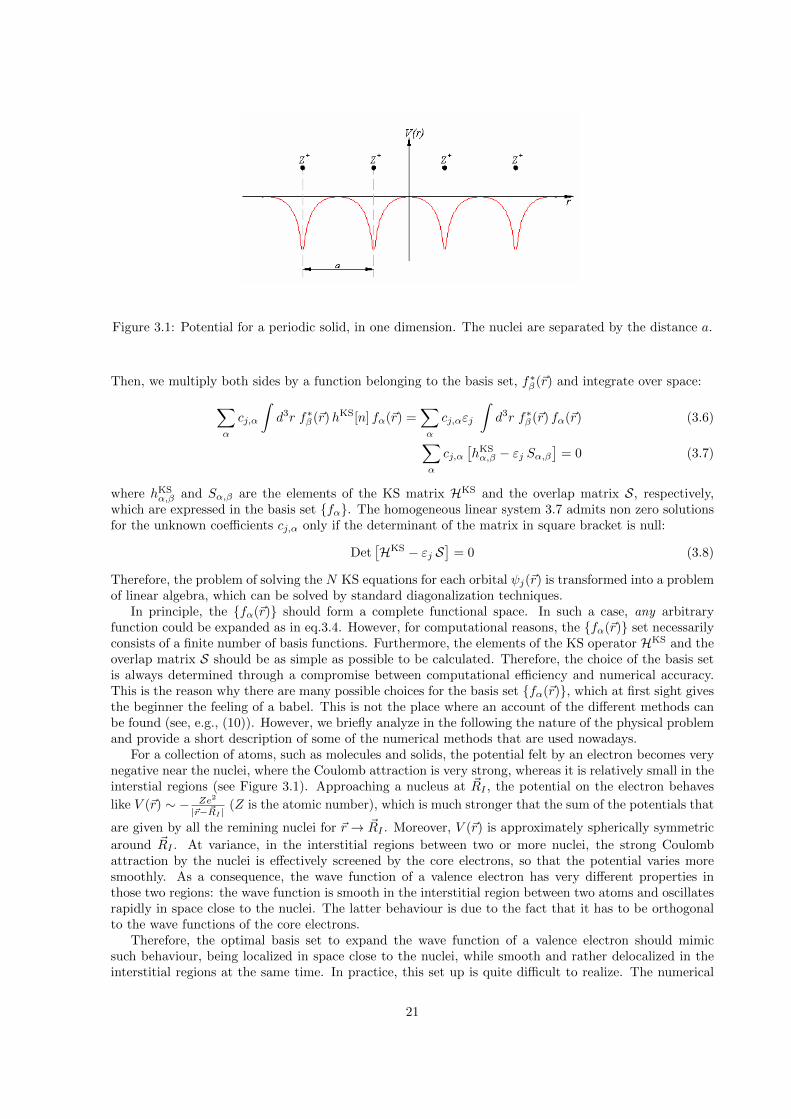
Figure 3.1: Potential for a periodic solid, in one dimension. The nuclei are separated by the distance a.

Then, we multiply both sides by a function belonging to the basis set, f∗β(~r) and integrate over space:∑α

cj,α

∫d3r f∗β(~r)hKS[n] fα(~r) =

∑α

cj,αεj

∫d3r f∗β(~r) fα(~r) (3.6)∑

α

cj,α[hKSα,β − εj Sα,β

]= 0 (3.7)

where hKSα,β and Sα,β are the elements of the KS matrix HKS and the overlap matrix S, respectively,

which are expressed in the basis set fα. The homogeneous linear system 3.7 admits non zero solutionsfor the unknown coefficients cj,α only if the determinant of the matrix in square bracket is null:

Det[HKS − εj S

]= 0 (3.8)

Therefore, the problem of solving the N KS equations for each orbital ψj(~r) is transformed into a problemof linear algebra, which can be solved by standard diagonalization techniques.

In principle, the fα(~r) should form a complete functional space. In such a case, any arbitraryfunction could be expanded as in eq.3.4. However, for computational reasons, the fα(~r) set necessarilyconsists of a finite number of basis functions. Furthermore, the elements of the KS operator HKS and theoverlap matrix S should be as simple as possible to be calculated. Therefore, the choice of the basis setis always determined through a compromise between computational efficiency and numerical accuracy.This is the reason why there are many possible choices for the basis set fα(~r), which at first sight givesthe beginner the feeling of a babel. This is not the place where an account of the different methods canbe found (see, e.g., (10)). However, we briefly analyze in the following the nature of the physical problemand provide a short description of some of the numerical methods that are used nowadays.

For a collection of atoms, such as molecules and solids, the potential felt by an electron becomes verynegative near the nuclei, where the Coulomb attraction is very strong, whereas it is relatively small in theinterstial regions (see Figure 3.1). Approaching a nucleus at ~RI , the potential on the electron behaves

like V (~r) ∼ − Ze2

|~r−~RI |(Z is the atomic number), which is much stronger that the sum of the potentials that

are given by all the remining nuclei for ~r → ~RI . Moreover, V (~r) is approximately spherically symmetric

around ~RI . At variance, in the interstitial regions between two or more nuclei, the strong Coulombattraction by the nuclei is effectively screened by the core electrons, so that the potential varies moresmoothly. As a consequence, the wave function of a valence electron has very different properties inthose two regions: the wave function is smooth in the interstitial region between two atoms and oscillatesrapidly in space close to the nuclei. The latter behaviour is due to the fact that it has to be orthogonalto the wave functions of the core electrons.

Therefore, the optimal basis set to expand the wave function of a valence electron should mimicsuch behaviour, being localized in space close to the nuclei, while smooth and rather delocalized in theinterstitial regions at the same time. In practice, this set up is quite difficult to realize. The numerical

21

methods that are used nowadays may be divided into few big classes: First, those that adopt basisfunctions that are localized in space (atomic functions, gaussians, etc.). Second, methods that employdelocalized functions, such as plane waves (they will be treated more extensively). Third, those thatmake use of both localized and delocalized functions, which are either constructed by superposition ofelementary functions (such as linear methods known as LMTO or FLAPW, or, more recently, PAW)or by adopting wavelets, which show a localized an delocalized character at the same time, as basisfunctions. It would be impossible to describe all of them, so that we limit ourselves to describe themethods that are based on plane waves in conjunction with pseudopotentials (section 3.1.2). This choiceis not motivated by the fact that they are the most performing ones (indeed, they aren’t!), but rather byconvenience: in fact, a pseudopotential-plane wave code will be used to compute material properties inthe hands-on-computer sessions.

3.1.1 Pseudo-potentials

Active electrons versus spectator electrons. In many problems in chemistry and physics, a distinc-tion between active and spectator electronic orbitals can be made. The problem can thus be formulatedin terms of the active electron wave-functions, while the spectator electrons can be treated within suitableapproximations. This concept is very general and lies at the hearth of any simplified model to simulateelectron systems. Among the criteria used to distinguish between active and spectator electrons, some areparticularly general and relevant in most cases : (A) The spectator and active electron energy scales mustdiffer considerably, by one order of magnitude or more; (B) They should react very unlikely to electronicperturbations; (C) Their respective density distributions are mostly localized in different regions of space.

If one is interested in the cohesive properties of condensed matter systems (solids, liquids, surfaces andinterfaces, large molecules and clusters ), a distinction between active electrons and spectator electrons isquite natural. The outer (valence) electrons are indeed responsible for the chemical behavior, while theinner electrons can be considered, in a first approximation, as inert. Core electron orbitals lie in energywell below the valence orbitals (of about -10n Hartree, with n ≥ 1), they are atomic-like, with a smallspatial extent and large gradients 1. All these features imply that the core orbitals are less polarizablethan the valence ones (11). Moreover, the chemical behavior of real materials is essentially determinedby bond breaking or formation, in which the inner orbitals do not play a crucial role.

In the pseudo-potential plane-wave approach, the core orbitals are frozen in their atomic state andthe action of the core electrons on the valence electron wave-functions is represented by means of suitableoperators, the pseudo-potentials; the valence electron orbitals are then expanded in plane waves.

Pseudopotentials: basic ideas. In order to understand some concepts that will be presented in thefollowing (non locality, non uniqueness, smoothness, etc.), it is useful to remind the original formulation ofthe pseudo-potential in condensed matter systems (12). The all-electron valence orbital |ψv〉 is representedas a linear combination

|ψv〉 = |φv〉+∑c

αcv|ψc〉 (3.9)

of a smooth wave-function |φv〉 and core electron orbitals |ψc〉 with suitable coefficients to ensure theorthogonality among core and valence orbitals. By considering that |ψv〉 and |ψc〉 are solution of theSchrodinger equation with eigenvalues εv and εc, respectively, one can easily obtain the equation for |φv〉: [

H +∑c

(εv − εc)|ψc〉〈ψc|

]|φv〉 = εv|φv〉 (3.10)

In equation 3.10, a smooth valence wave-function |φv〉 is the lowest-energy solution of a new Hamiltonian,with the same eigenvalue as the all-electron valence wave-function |ψv〉. The new Hamiltonian containsthe additional projector ℘ =

∑c(εv − εc)|ψc〉〈ψc| which is non-local, that is, cannot be represented as

a multiplicative term. Moreover, such a term is repulsive – which can be seen by considering that thematrix element 〈φv|℘|φv〉 is positive definite – and short-range, like the core orbitals. By replacing theall-electron problem with an effective Hamiltonian acting on smooth wave-functions that describe thevalence electrons, the computational load is alleviated in two respects. First, we reduce the number of

1As a consequence, their expansion in terms of delocalized functions such as plane waves is problematic.

22

the self-consistent KS orbitals to be determined. Second, we avoid representing the rapid oscillations ofthe all-electron valence orbitals close to the nucleus explicitly, while keeping the long tails that are mainlyresponsible for the formation of the chemical bonds.

The actual choice of pseudo-potentials that are employed to replace the core electrons is connectedto the basis set used to represent the valence orbitals. In particular, when using a plane-wave basis set,the pseudo-potential should be soft, which means that its Fourier-transform should decrease as fast aspossible with the magnitude of the wave-vector. Therefore,the expansion of a soft pseudopotential needsless plane-waves than a hard one, which is clearly advantageous from the computational point of view.

However, one must remark other important features of such an approach:

(a) The pseudo wave function |φv〉 as defined in equation 3.9 is not normalized.

(b) The choice of |φv〉 is not unique, which implies that the operator ℘ is not unique, too (see thecorresponding exercise).

(c) The projector operator acts differently on the different angular momenta that are present in the core:℘ =

∑n,l,m∈core(εv − εnlm)|ψnlm〉〈ψnlm| = ℘s + ℘p + ...

Norm-conserving pseudopotentials. An important class of pseudo-potentials, which are still cur-rently used, are the so-called norm-conserving pseudo-potentials. Along the hands-on-computer sessions,they will be given as an input for the numerical projects. A short description is given in the following.The interested reader is referred to (10) for more details on their generation and their use. Let us consideran isolated atom in the Coulomb potential. The solutions of the corresponding Kohn-Sham equation canbe written as:

ψnlm(~r) = Ylm(θ, ϕ)χnl(r) (3.11)

where n, l and m are the principal, angular and azimuthal quantum numbers, respectively. To be morespecific, let us consider a particular atom, for instance Al. Its atomic structure is (1s)2(2s)2(2p)6(3s)2(3p)1.Firstly, we choose as core (spectator) electrons those belonging to the complete (1s)2(2s)2(2p)6 shells, andthe 3s and 3p electrons in the valence. The valence charge of the pseudo-atom is thus Zval = 3. The all-electron χ3s(r) wave function has two nodes (see figure); we replace it with a nodeless, smoother pseudowave function, which coincides with the all-electron one for r > rc ' 1.5a0 (a0 is the Bohr radius of the H

atom). Therefore, the all-electron equation Hχ3s = ε3sχ3s is replaced with H(ps)3s χ

(ps)3s = ε3sχ

(ps)3s . Since

χ(ps)3s is nodeless, the previous equation can be inverted and V

(ps)3s (r) computed. Obviously, the same

procedure must be used to build a pseudopotential that corresponds to 3p states. χ(ps)3s is normalized

exactly as χ3s, which is the reason why the pseudpotentials are said to be norm-conserving. The resultingoperator can thus be represented as:

V (ps) =

lmax∑l=0

l∑m=−l

V(ps)l (r)|Ylm〉〈Ylm| (3.12)

that is, as a sum of multiplicative terms in r and operators on the angular components. Basically, V(ps)l (r)

behaves like −Zvale2

r for r > rc ∀l, while it differs sensitively for different angular components in the coreregion, r ≤ rc. This is because the core states have a distinct behaviour for each l, and so do thepseudo-wave functions and the corresponding pseudo-potential.

3.1.2 Plane waves

The direct and reciprocal spaces. A perfect (ideal) crystal is a collection of atoms that are regularlyplaced on a three-dimensional lattice with long-range order. Because of the translational symmetry, theknowledge of the atomic structure within the elementary unit cell suffices to know the whole crystalstructure. More precisely, any lattice point ~rl is given by linear combinations of the primitive latticevectors ~a1,~a2, ~a3, which form a linear space, the direct space:

~rl =

3∑i=1

li~ai (3.13)

23

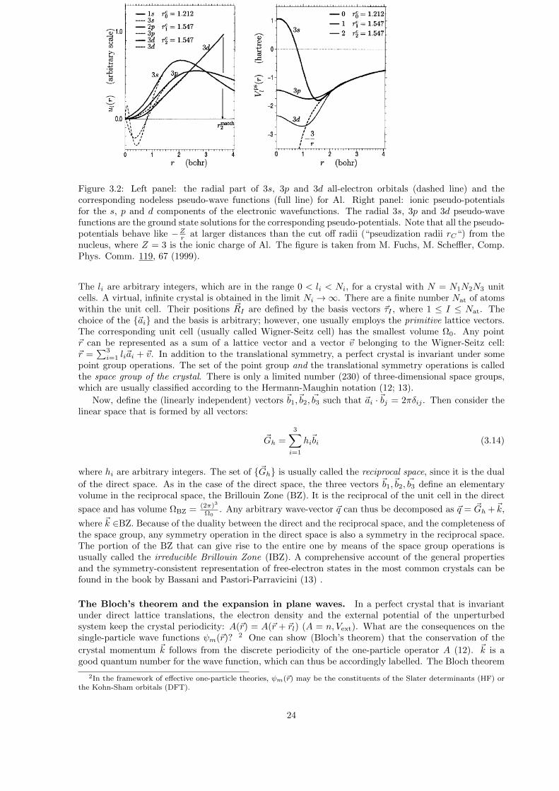
En pratique (2)

Figure 3.2: Left panel: the radial part of 3s, 3p and 3d all-electron orbitals (dashed line) and thecorresponding nodeless pseudo-wave functions (full line) for Al. Right panel: ionic pseudo-potentialsfor the s, p and d components of the electronic wavefunctions. The radial 3s, 3p and 3d pseudo-wavefunctions are the ground state solutions for the corresponding pseudo-potentials. Note that all the pseudo-potentials behave like −Zr at larger distances than the cut off radii (“pseudization radii rC“) from thenucleus, where Z = 3 is the ionic charge of Al. The figure is taken from M. Fuchs, M. Scheffler, Comp.Phys. Comm. 119, 67 (1999).

The li are arbitrary integers, which are in the range 0 < li < Ni, for a crystal with N = N1N2N3 unitcells. A virtual, infinite crystal is obtained in the limit Ni →∞. There are a finite number Nat of atomswithin the unit cell. Their positions ~RI are defined by the basis vectors ~τI , where 1 ≤ I ≤ Nat. Thechoice of the ~ai and the basis is arbitrary; however, one usually employs the primitive lattice vectors.The corresponding unit cell (usually called Wigner-Seitz cell) has the smallest volume Ω0. Any point~r can be represented as a sum of a lattice vector and a vector ~v belonging to the Wigner-Seitz cell:~r =

∑3i=1 li~ai + ~v. In addition to the translational symmetry, a perfect crystal is invariant under some

point group operations. The set of the point group and the translational symmetry operations is calledthe space group of the crystal. There is only a limited number (230) of three-dimensional space groups,which are usually classified according to the Hermann-Maughin notation (12; 13).

Now, define the (linearly independent) vectors ~b1,~b2, ~b3 such that ~ai ·~bj = 2πδij . Then consider thelinear space that is formed by all vectors:

~Gh =

3∑i=1

hi~bi (3.14)

where hi are arbitrary integers. The set of ~Gh is usually called the reciprocal space, since it is the dual

of the direct space. As in the case of the direct space, the three vectors ~b1,~b2, ~b3 define an elementaryvolume in the reciprocal space, the Brillouin Zone (BZ). It is the reciprocal of the unit cell in the direct

space and has volume ΩBZ = (2π)3

Ω0. Any arbitrary wave-vector ~q can thus be decomposed as ~q = ~Gh +~k,

where ~k ∈BZ. Because of the duality between the direct and the reciprocal space, and the completeness ofthe space group, any symmetry operation in the direct space is also a symmetry in the reciprocal space.The portion of the BZ that can give rise to the entire one by means of the space group operations isusually called the irreducible Brillouin Zone (IBZ). A comprehensive account of the general propertiesand the symmetry-consistent representation of free-electron states in the most common crystals can befound in the book by Bassani and Pastori-Parravicini (13) .

The Bloch’s theorem and the expansion in plane waves. In a perfect crystal that is invariantunder direct lattice translations, the electron density and the external potential of the unperturbedsystem keep the crystal periodicity: A(~r) = A(~r + ~rl) (A = n, Vext). What are the consequences on thesingle-particle wave functions ψm(~r)? 2 One can show (Bloch’s theorem) that the conservation of the

crystal momentum ~k follows from the discrete periodicity of the one-particle operator A (12). ~k is agood quantum number for the wave function, which can thus be accordingly labelled. The Bloch theorem

2In the framework of effective one-particle theories, ψm(~r) may be the constituents of the Slater determinants (HF) orthe Kohn-Sham orbitals (DFT).

24

states that the wave function has the following property:

ψm,~k(~r + ~rl) = ei~k·~rl ψm,~k(~r) (3.15)

As a consequence, the wave function can be decomposed in a product of a phase factor by a functionum,~k having the crystal periodicity as:

ψm,~k(~r) =1√NΩ0

ei~k·~rum,~k(~r) with um,~k(~r + ~rl) = um,~k(~r) (3.16)

The periodic function um,~k(~r) is expanded in a discrete sum over the reciprocal lattice vectors as:

um,~k(~r) =∑~G

ei ~G·~r um(~k + ~G) (3.17)

The um(~k + ~G) are the Fourier coefficients in the wavevector space. Since ~k is a good quantum number,

there are as many distinct expansions 3.17 as the number of ~k points within the IBZ. 3 From the definitionof the reciprocal lattice vectors ~G (equation 3.14) and the construction of the basis vectors of the two

linear spaces (~ai · ~bj = 2πδij), it is straightforward to verify that the expansion 3.17 guarantees thatum,~k(~r + ~rl) = um,~k(~r) ∀ ~rl.

In principle, any function having the lattice periodicity can be expanded according to equation 3.17,since the plane waves form a complete basis set. However, the expansion 3.17 contains an infinite numberof terms, which is not feasible for numerical applications on a computer. From the basic principlesof Fourier analysis, the need of including wave vectors of increasing magnitude is connected to thesmoothness of the function to be expanded: the more smooth the function, the faster the expansionconverges. Functions that vary rapidly in space need a very large number of wave vectors when expandedin plane waves. Therefore, the sum in 3.17 is generally rearranged summing up over wave vectors of

increasing magnitude. Then, it is cut off, by excluding wave vectors such that ~2|~k+~G|22m > Ecut:

um,~k(~r) =∑

~G: ~2|~k+~G|2

2m ≤Ecut

ei ~G·~r um(~k + ~G) (3.18)

Ecut is the maximum allowed kinetic energy of the plane waves involved in the truncated sum 3.18 andis a crucial parameter. On one hand, the larger Ecut, the better is the quality of the basis set, whichtends to a complete one. 4 On the other hand, the smaller Ecut, the smaller is the number of Fouriercoefficients to be calculated and stocked in the computer memory. As a consequence, Ecut is determinedthrough a compromise between numerical accuracy and computational burden. In practice, Ecut is theonly parameter that adjusts the qualty of the PW basis set. The choice is usually done by looking tothe behavior of several quantities (total energy, structural parameters, electronic structure, etc.) as afunction of Ecut. As soon as they converge reasonably, the optimal Ecut is determined.

Born-Von Karman boundary conditions and BZ sampling. Consider a finite system with aninteger number N = N1N2N3 of unit cells. In order to simulate an infinite periodic system, the Born -von Karman (BvK) cyclic boundary conditions are often used:

ψm,~k(~r + Ni ~ai) = ψm,~k(~r) (3.19)

m and ~k label the band and the wave-vector, respectively. Because of the BvK conditions, the number of~k wave-vectors in the BZ is equal to N = N1N2N3 and their density to Ω0/(2π)3. Therefore, as the size

of the system increases, the ~k points become dense in the BZ and tend to be infinite for a truly unboundcrystal. Clearly, there are computational restrictions that prevent the use of a too large set of ~k points.The choice of an optimal finite set is often referred to as BZ sampling.

3Since ~k and ~G are homogeneous, the Fourier coefficient um(~k + ~G) is a function of the generic wavevector ~q = ~k + ~G.4Roughly speaking, Ecut fixes the wave vector with the largest allowed magnitude, let’s say Gmax. The resolution in

the direct space, that is, the distance between two points in the real space grid, is 2πGmax

, as it can be easily proved (see

exercise).

25

In practice - apart from the case in which the dependence on a particular wave-vector ~k must beexplicitly known - one has to compute averages of ~k-dependent functions over the BZ:

f =Ω

(2π)3

∫BZ

d3k f(~k) . (3.20)

In this case, the average f is assumed to be a c-number, such as the expectation value of the kinetic energyoperator in the DFT. In other cases, the function f depends on the other coordinates – for instance, theelectron density in the DFT is computed through a sum over the BZ of a non-negative function definedin the real space. For such cases, several schemes have been proposed to consider as few as possible ~kpoints in the BZ and thus reduce the computational cost. Among them, the special point technique (9)and the tetrahedron method are the most popular ones.

In the special point technique, the average of f over the BZ (Equation 3.20) can be approximated by

a weighted sum over a finite number N~k of ~k points:

f =

N~k∑i=1

w~kif(~ki) + e(~ki) (3.21)

with normalized weights:∑w~ki = 1. For a given Nk, the set of special points ~ki is such that the

error e(~ki) is minimized. A demonstration, which is based on the use of the lattice point group of

the crystal and the symmetry of f(~k) for translations by reciprocal lattice vectors, can be found in thepaper by Chadi and Cohen (14). In the same paper, a method for generating the special point sets isoutlined and the determination of various special point sets explicitly carried out for cubic and hexagonalcrystal lattices. A more general method for generating equispaced grids of ~k points for crystals of anysymmetry, which is equivalent to that introduced by Chadi and Cohen in special cases, was then providedby Monkhorst and Pack (15).

The special point technique is well suited for integrating smoothly varying functions in the BZ,particularly for insulators and semiconductors, where the number of occupied bands is independent ofthe wavevector ~k, which simplifies its practical implementation. In metals, the number of occupied bandscan vary abruptly with ~k, as a consequence of band crossing, and the shape of the Fermi surface may becomplicated and generally admits singular points. A practical way to deal with such singularities is tosmoothen the Fermi surface by replacing the Heaviside function in Equation 2.9 with a smeared occupationfunction s(εF − εm,~k; α) where the set of parameters α defines the actual choice of smearing (9). Asimple example is provided by the Fermi-Dirac distribution, the width of which around εF is proportionalto the temperature T . However, all physical quantities must generally be computed in the limit of nosmearing (e.g. T → 0 in the Fermi-Dirac distribution) in order to avoid the arbitrariness linked to thechoice of the function s.

An alternative approach to sample the BZ is provided by the tetrahedron method (9), which is basically

a simplex method for interpolating f(~k). The irreducible part of the BZ is partitioned into tetrahedra,

within which f(~k) is linearized in ~k. The linear approximation allows the integration (Eq.3.20) to becomputed analytically, taking into account the complicated shape of the Fermi surface. While there arefew doubts that at zero temperature the tetrahedron method is superior to the special point techniquein metals, for insulators the latter one is often computationally faster and more robust.

The computation of electronic spectra in crystals, in contrast, represents a different picture. In thiscase, it is preferable to sample the BZ by using ~k points that do not have any special symmetry. Indeed,the electronic bands may be flat or degenerate in highly symmetric ~k points, which would artificiallyreinforce the computed weight of such electronic transitions. A practical alternative in those cases is togenerate a special point grid that is successively shifted from the BZ center by a linear combination ofthe reciprocal lattice vectors with small coefficients, of the order of few tenths.

How to treat aperiodic systems. Obviously, not all the interesting physical systems are perfectcrystals! On the contrary, since the advent of nano-sciences, there is a growing interest for systems thathave one or more dimensions in the nanometer range, such as interfaces, graphene, supported clusters,nanowires and nanodots. Those systems are truly aperiodic and their properties are very much linked totheir reduced dimensions. In principle, plane waves are not well suited for treating such cases, since their

26

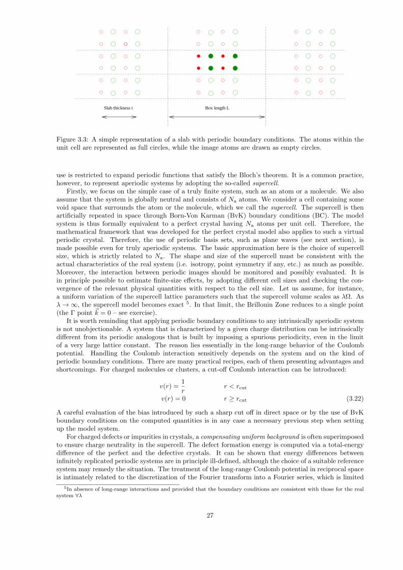
Box length LSlab thickness t

Figure 3.3: A simple representation of a slab with periodic boundary conditions. The atoms within theunit cell are represented as full circles, while the image atoms are drawn as empty circles.

use is restricted to expand periodic functions that satisfy the Bloch’s theorem. It is a common practice,however, to represent aperiodic systems by adopting the so-called supercell.

Firstly, we focus on the simple case of a truly finite system, such as an atom or a molecule. We alsoassume that the system is globally neutral and consists of Na atoms. We consider a cell containing somevoid space that surrounds the atom or the molecule, which we call the supercell. The supercell is thenartificially repeated in space through Born-Von Karman (BvK) boundary conditions (BC). The modelsystem is thus formally equivalent to a perfect crystal having Na atoms per unit cell. Therefore, themathematical framework that was developed for the perfect crystal model also applies to such a virtualperiodic crystal. Therefore, the use of periodic basis sets, such as plane waves (see next section), ismade possible even for truly aperiodic systems. The basic approximation here is the choice of supercellsize, which is strictly related to Na. The shape and size of the supercell must be consistent with theactual characteristics of the real system (i.e. isotropy, point symmetry if any, etc.) as much as possible.Moreover, the interaction between periodic images should be monitored and possibly evaluated. It isin principle possible to estimate finite-size effects, by adopting different cell sizes and checking the con-vergence of the relevant physical quantities with respect to the cell size. Let us assume, for instance,a uniform variation of the supercell lattice parameters such that the supercell volume scales as λΩ. Asλ→∞, the supercell model becomes exact 5. In that limit, the Brillouin Zone reduces to a single point(the Γ point ~k = 0 – see exercise).

It is worth reminding that applying periodic boundary conditions to any intrinsically aperiodic systemis not unobjectionable. A system that is characterized by a given charge distribution can be intrinsicallydifferent from its periodic analogous that is built by imposing a spurious periodicity, even in the limitof a very large lattice constant. The reason lies essentially in the long-range behavior of the Coulombpotential. Handling the Coulomb interaction sensitively depends on the system and on the kind ofperiodic boundary conditions. There are many practical recipes, each of them presenting advantages andshortcomings. For charged molecules or clusters, a cut-off Coulomb interaction can be introduced:

v(r) =1

rr < rcut

v(r) = 0 r ≥ rcut (3.22)

A careful evaluation of the bias introduced by such a sharp cut off in direct space or by the use of BvKboundary conditions on the computed quantities is in any case a necessary previous step when settingup the model system.

For charged defects or impurities in crystals, a compensating uniform background is often superimposedto ensure charge neutrality in the supercell. The defect formation energy is computed via a total-energydifference of the perfect and the defective crystals. It can be shown that energy differences betweeninfinitely replicated periodic systems are in principle ill-defined, although the choice of a suitable referencesystem may remedy the situation. The treatment of the long-range Coulomb potential in reciprocal spaceis intimately related to the discretization of the Fourier transform into a Fourier series, which is limited

5In absence of long-range interactions and provided that the boundary conditions are consistent with those for the realsystem ∀λ

27

to reciprocal lattice vectors. By isolating the long-range contribution, which can be treated analytically,from the short-range one, which depends on the local details of the charge distribution and can becomputed numerically, some ways of dealing with the Coulomb interaction in systems with periodicboundary conditions have been devised.

Another important case is provided by systems that are periodic in one or two dimensions and ape-riodic in the remaining ones. A classical example is provided by surfaces. They are simulated by a slabconsisting of some atomic layers, plus a surrounding vacuum region, with periodic boundary conditionsalong the surface plane (see Figure 3.1.2). The slab has to be thick enough to display the bulk character-istics (atomic positions, electronic structure, etc.) in the innermost layers. Despite the finite thickness, itis possible to extract convergent surface energies from this kind of calculations. The safest way, althoughnot the most economic one as far as the computing time is concerned, is to increase the slab thicknesst systematically, starting from a minimum t that allows bulk properties to be properly defined 6. Theslab total energy is then plotted as a function of the number of layers Nl, so that the averaged surfaceenergy over the two slab terminations can be extrapolated at Nl = 0 However, especially when using aplane wave basis set (see Section 4.4), periodic boundary conditions are imposed along the normal to thesurface plane, which can be source of numerical errors. This is the case, for example, of slabs with a netdipole moment, which give rise to intrinsically non-periodic electrostatic potentials. A way to overcomesuch difficulties still using 3-D PBC has been recently discussed.

The KS hamiltonian in plane waves. Here we provide a simple example on how the total energyand electron density are computed in plane waves. We will not be exhaustive, but give the simplestformulae to serve as a guideline. For those who wish to deeper their knowledge, a thorough account canbe found in many books and articles (9).

First, we recall the expression of the Kohn-Sham orbitals in plane waves for a spin-compensatedsystem of N electrons:

ψm,~k(~r) =∑~G

ei (~k+~G)·~r um(~k + ~G) (3.23)

where m is the band index and ~k the crystal momentum. The electron density is given in terms of theKohn-Sham orbitals as:

n(~r) = 2∑m

∑~k

w~k fm,~k | ψm,~k(~r) |2 (3.24)

where w~k is the weight of each ~k point that sample the Brillouin zone, and fm,~k is the occupation factor

(according to the Fermi-Dirac statistic or whatever), which ranges between 0 and 1. The factor 2 accountsfor spin degeneracy.

If we replace in equation 3.24 the Kohn-Sham orbitals ψm,~k(~r) by their plane wave expansion 3.23,the electron density would be computed through a double sum over the reciprocal space. Generally,the number of PW’s MPW is large, making the straightforward calculation of n(~r) scaling as NM2

PW

and becoming rather slow. However, we can adopt another faster and smarter method, which relies onthe properties of Fast Fourier Transforms (FFT). For each point ~k and each band m, starting from the

knowledge of the Fourier coefficients um(~k+ ~G), we compute through the inverse FFT the correspondingperiodic part of the KS orbital um,~k(~r). The computational load of such an operations is MPW logMPW.Next, we compute its square modulus and sum up over the Nk points in the BZ and the occupied orbitals,which are ' N , obtaining the electron density in direct space via equation 3.24. Once n(~r) is computed,

its Fourier coefficients in the reciprocal space n(~G) can be determined via direct FFT. Global scaling ofsuch procedure is ∼ NNkMPW logMPW, thus much better than the double sum in reciprocal space.

Regarding the calculation of the total energy, some terms can be evaluated in the reciprocal space,while some others in the direct space. First, we rewrite equation 2.27:

E[n] = Ts[n] +

∫d3r Vext(~r)n(~r) + EH[n] + Exc[n] (3.25)

6Please note that the space group of the slab is generally different from that of the infinite crystal. Therefore, one hasto preoceed carefully when considering the reference bulk state.

28

where Ts[n] is the kinetic contribution of a virtual non interacting system with density n(~r), EH[n] is theclassic Hartree contribution to the electron-electron interaction, and Exc[n] is written in the LDA, forsimplicity sake:

Ts[n] = 2∑m

∑~k

w~kfm,~k

∫d3r ψ∗

m,~k(~r)

[−~2∇2

2mψm,~k(~r)

](3.26)

EH[n] =e2

2

∫d3r

∫d3r′

n(~r)n(~r′)

|~r − ~r′|(3.27)

Exc[n] ' ELDAxc [n] =

∫d3r n(~r) eHEG

xc (n(~r)) (3.28)

Once the electron density n(~r) is determined as explained above, ELDAxc [n] is easily computed in the

direct space. On the contrary, the Hartree contribution involves a double integral in direct space, whichalso contains the factor |~r − ~r′|−1, which may diverge for arbitrarily close points. Making use of someanalytical skill (see exercise), EH[n] can be conveniently rewritten in the reciprocal space as:

EH[n] = 2πΩ0

∑G6=0

|n(~G)|2

G2(3.29)

The sum over the reciprocal lattice vectors (~G) excludes the diverging term ~G = 0. It can be shown thatsuch a long-wavelenght divergence does not take place in globally neutral system, for which the positivecharges, given by the ions, are equal to the number of electrons. Equation 3.29 provides a very simpleand fast way to compute EH[n], which scales as MPW.

We end this section by summarizing the main characteristics of plane waves, pros (+) and cons (-):

+ Plane waves expansion is equivalent to interpolate functions (orbitals, density and potential) interms of sinus and cosinus that have the lattice periodicity. The precision is the same everywhere,independently of the atomic positions. The improvement of the quality of the basis set is particularlysimple to be done by increasing just one parameter, the cutoff on the wave vector energy.

+ Different quantities can be computed either in the direct space or in the reciprocal space, accordingto the computational convenience. Plane waves based codes are thus quite easy to be written andimplemented. The use of fast-Fourier transforms makes very simple and effective to go back andforth between the two dual spaces.

+ The quality of the basis set is independent of the atomic positions. Therefore, the computation ofenergy derivatives with respect to the atomic positions (i.e. the forces on the atoms) is very simpleand safe. Moreover, PW’s can describe the electron density in regions of space where there are nonuclei, at odds with localized basis sets.

- Plane waves are generally used in conjunction with pseudo-potentials, so that close to the nucleithe orbitals are different from their all-electron counterparts.

- Many plane waves are commonly employed in the expansion, typically around 102 per electronpair (obviously, the precise number depends on the pseudopotentials, the cut off energy, etc.).The interpretation of the expansion coefficients is not physically intuitive and files handling iscumbersome.

- PW’s are used in conjunction with periodic boundary conditions, which poses problems for charged,non periodic systems. These systems are simulated by adopting supercells with void space, whichincreases the computational burden.

29

Exercises

1. BvK conditions in one dimension. The case of very large cells and Gamma point.

2. A single electron in a potential well of varying deepness.

3. Uniqueness of pseudo-potentials.

3.2 Solving the Kohn-Sham equations: the self-consistent cycle

As mentioned at the beginning of this chapter, the Kohn-Sham equations must be solved self-consistently,which is usually achieved by iterations. Starting from a trial density n(0)(~r) (which can be obtained fromtrial orbitals), hKS[n(0)] is constructed according to equation 3.3. Then, the KS equation 3.1 is solved

and new KS orbitals ψ(1)j are obtained. A new density n(1)(~r) is thus computed according to equation

3.2. From n(1)(~r) a new KS effective one-electron hamiltonian is derived, and so on. The process goeson until the differences of the KS effective one-electron hamiltonians at two successive iterations (or theelectron densities) are below a pre-determined small number. Therefore, the solution of the KS equationsis find when the input and output effective potential (or the electron density) coincide with each other.In other word, if we apply the KS machinery to a given function v, we want that the result to be v again.Mathematically, if K represents the ensemble of the operations that allow v to be recalculated accordingto the KS equations, we require that

v = K(v) (3.30)

that is, we must find the fixed point v for the application K. Finding the fixed points of a generalapplication, defined on a linear space, is a common mathematical problem. Many numerical approachesare available, where the solution is attained through iterations. However, it is not the scope of thepresent section to give a comprehensive account of these methods. Rather, we focus on selected examplesshowing why the convergence to the self-consistent solution may be delicate and rather time-consuming.The reader should consult ”The Computational Physicist’s Toolkit” by Philippe Depondt (chapter 3.2),where a few other examples are presented and discussed.

First of all, we imagine to have already found the fixed point of the application, such that v0 = K(v0).What happens if we move a little away from the solution? Let’s try with v = v0 + δv, with small δv. 7

K(v0 + δv) = K(v0) + δv

[∂K

∂v

]0

+ . . . (3.31)

or, in other words:

δK = K(v0 + δv)−K(v0) '[∂K

∂v

]0

δv (3.32)

There are two different cases: if |[∂K∂v

]0| < 1, δK < δv. The new value v1 = K(v0 + δv) thus satisfies:

|v1 − v0| < |δv|. The sequence v1, v2, . . . , vn would thus converge to v0 as n grows and the fixed point

7Note that δv may also represent the numerical error when we approach the self-consistent solution.

30

v0 is said to be stable. Eventually, the convergence may be very slow if |[∂K∂v

]0' 0. In any case,

straightforward iterations of the application will lead us to the nearest fixed point; slowly, but surely! Onthe other hand, if |

[∂K∂v

]0| > 1, simple iterations of the application will lead to divergence. In such a case,

the fixed point is unstable: an arbitrary small perturbation to the solution would drive the system faraway from the fixed point. This is actually the case of the KS cycle, for most physical problems. Beforediscussing the reasons that underlie such a divergence, I would like to anticipate that, even for divergingapplications K (that is, those for which |

[∂K∂v

]0| > 1), it is always possible to define a new application,

let’s say K ′, which has a stable fixed point. That’s very simple! Let choose a positive number p suchthat 0 < p < 1

max |[ ∂K∂v ]0|, where the max is taken among all the directions of the derivative (v is supposed

to be an element in a vector space of dimension >1, or even a functional space, with infinite dimension).Then define the new application:

K ′(v) = pK(v) + (1− p)v (3.33)

which is a simple mixing of the input v and the output K(v). It is straightforward to verify that K ′

has the same fixed point v0 as K and that it is now stable, that is, |[∂K′

∂v

]0| < 1. The numerical

scheme in equation 3.33 is usually referred to as simple mixing. This is a very robust algorithm to attainconvergence! However, it can be shown that the convergence becomes very slow as p → 0; an examplecan be found in the aforementioned book by Ph. Depondt.

Why is the KS fixed point unstable? Clearly, one should linearize the KS application and find itsderivative around the fixed point. However, each particular system has a distinct ground state densityn(~r) and effective potential Vs(~r), as guaranteed by the Hohemberg-Kohn theorem. Therefore, it is adifficult task to derive general and rigorous criteria that are valid for any system of N electrons subjectto an external potential. Rather, I will take an example from electrostatics, which is well suited to showthe root of the instability. Consider a classical set of negative charges (they mimic the electrons) that aresubject to a stabilizing external potential. This is a common electrostatic problem, which is equivalentto minimize:

E[n] = −e∫d3r

[1

2V (~r) + Vext(~r)

]n(~r) (3.34)

where

V (~r) = −e∫d3r′

n(~r′)

|~r − ~r′|(3.35)

and the external potential may be thought as generated by a given (fixed) positive charge distributionn+(~r):

Vext(~r) = e

∫d3r′

n+(~r′)

|~r − ~r′|(3.36)

The above relation between the negative charge density n and the electrostatic potential V is the solutionof the Poisson equation 8:

∇2 [V (~r) + Vext(~r)] = 4πe [n+(~r)− n(~r)] (3.37)

which can be more easily analysed by passing to the wave vector space ~q through Fourier transforms:

q2[V (~q) + Vext(~q)

]= 4πe [n+(~q)− n(~q)] (3.38)

which has the solution:

V0(~q) = −Vext(~q) + 4πen+(~q)− n0(~q)

q2(3.39)

8Here we use the so called Gaussian units. In these units, Maxwell’s first equation equation for the electric displacement~D(~r) in terms of the total charge distribution ρ(~r) reads ∇ · ~D = 4πρ; the relation between ~D(~r), electric field ~E(~r) and

polarization c(~r) is ~D = ~E + 4π ~P . In Gaussian units the void electric permittivity is simply ε0 = 1 and the void magnetic

constant µ0 = 1; as ε0µ0 = c−2, with c the speed of light, the Lorentz force per unit charge is ~F = ~E + ~vc× ~B. This could

be compared to the same equations in the MKSA unit system: ∇ · ~D = ρ; ~D = ε0 ~E + ~P and ~F = ~E + ~v × ~B; the void

electric permittivity is ε0 = 107

4πc2.

31

The above equation represents the self-consistent relation between the charge distribution n and the elec-trostatic potential V it generates by mutual repulsion between the negatively charged classical particles.It can be easily linearized around the fixed point giving:

δV (~q) = −4πeδn0(~q)

q2(3.40)

It is important to focus on the previous equation by distinguishing two cases:

• The case of short wave lengths (or large wave vector q). In such a case, any fluctuation around theexact solution produces smaller fluctuations on the potential. The cycle will then converge to thestable fixed point.

• The case of long wave lengths (or small wave vector q). Any density fluctuation, such as an errorthat may be due to a lack of numerical precision, or an initial estimate that does not coincide withthe analytical solution, yields large fluctuations on the electrostatic potential. The simple iterationof equations 3.35 and 3.37 does not attain convergence. The fixed point is unstable.

Physically speaking, if a system has bigger dimensions than a characteristic length Lc ' [4πn]−1/3

,the long-range Coulomb interaction can produce oscillations in the electrostatic potential. Accordingly,the charge density, which is initially localized, let’s say in a region A, at the following iteration maybe localized in another portion of space, let’s say B, which is quite far from A. Such a phenomenon isusually called charge sloshing. There is a quite easy way to avoid charge sloshing, simply by introducinga threshold wavelength qcut ' 2π

Lc. The equation 3.40 that links the variation of the potential at the next

iteration δV (~q) as a function of the charge density fluctuations δn(~q) between the input and output n(~q)is modified as follows:

δV (~q) = −4πeδn(~q)

q2cut + q2

(3.41)

The cycle will then converge to the fixed point. The readers who know electron screening, would likelyrecognize a function that they have already seen, the Thomas-Fermi static dielectric function in reciprocal

space! Indeed, δV (~q) as given by 3.41 may be thought as a perturbation; the input potential V(n+1)in (~q)

for the next iteration n+ 1 would only uptake a part of it:

V(n+1)in (~q) = V

(n)in (~q) +

q2

q2cut + q2

[V

(n)out (~q)− V (n)

in (~q)]

(3.42)

which is equivalent to a simple mixing in the reciprocal space, with a q-dependent coefficient! Otherpopular, and usually more effective, mixing schemes are the Anderson and the Broyden methods. Theirimplementation for the Kohn-Sham problem is detailed in (17).

Another fundamental reason why the KS cycle may diverge is given to the presence of degeneratedor almost degenerated energy levels around the Fermi energy. For simplicity sake, imagine to have twoperfectly degenerated Kohn-Sham levels at the Fermi energy, that should be filled with two orbitals. Theobvious solution is that they must be both half-filled. However, they are degenerated only when theself-consistent solution is attained! Therefore, at the starting point, one of them (let’s say εA) would belower than the other (εB). If the filling rules at zero electronic temperature are assumed, level A willbe filled with two states, while B would be empty. At the following iteration, if the electron-electronrepulsion is strong enough, εA > εB and the reverse filling would result. The system would then goback and forth between these two states, without necessarily attaining convergence. A solution to such aproblem is to adopt a finite-temperature function for electron filling. Such a procedure is usually knownas Fermi-surface smearing. There are many available smearing schemes. A comprehensive account maybe found in (16).

Now, let’s come back to the Kohn-Sham problem and its numerical resolution. The KS cycle has twocharacteristics: first, the potential and electron density are constructed through the single-particle KSorbitals ψm. Each of them (there are about N , the number of electrons in the system) is expanded in abasis set, with M components. In the case of plane waves, the total number of degree of freedom may beNM ∼ 106 and even more! Therefore, any good algorithm should not make use of many vectors, sincethey are quite cumbersome. Second, the diagonalization of the KS hamiltonian is computationally verydemanding. A good algorithm should converge as fast as possible, in order to save computer time.

32

Conjugate gradient methods are widespreadly used for the minimization of the DFT total electronicenergy E given by equation 3.25. The principle of these kinds of algorithms is to find the optimal KSorbitals by relying on the generalized forces Fj = − δE

δψj. Iterations go on until Fj ' 0. Information on

the evolution of Fj as iterations proceed enables the construction of an approximate metric that should

tend towards the exact Hessian Hij = − δ2Eδψiδψj

. Since the KS orbitals are usually expanded on a basis

set, the Hessian has the same dimensions as the KS hamiltonian hKS. The convergence gets faster asthe gap between the biggest and smallest generalized forces shrinks. This is usually achieved by pre-conditioning : the Hamiltonian matrix is multiplied by a diagonal matrix Mp so that the smallest andlargest eigenvalues become closer in magnitude. When using PW’s, it is usual to consider the inverseof the kinetic energy as the pre-conditioning matrix Mp. A comprehensive account of pre-conditionedconjugate gradient methods can be found in (17).

Another popular and very effective scheme for minimizing ςj = 〈ψj |(hKS − εj)|ψj〉 9 is the so-called

Direct Inversion of Iterative Subspace method (DIIS). The self-consistent solution ψ(∞)j is written as a

linear combination of the KS orbitals at the previous iterations ψ(n)j . The optimal linear combination

is found by minimizing the residual ςj . A thorough account of the use of DIIS for the KS problem is

given in (18). The DIIS method is very effective whenever the KS orbitals ψ(n)j are relatively close to

the exact solution. Therefore, it is often used to refine the first guess, which has been found by otheralgorithms, such as conjugate gradients.

9Note that if ςj = 〈ψj |(hKS − εj)|ψj〉 = 0 ∀j self-consistency is attained. Therefore, the minimization of ςj is often usedas a criterion for convergence towards the self-consistent solution of the KS equations.

33

Chapter 4

Density Functional PerturbationTheory

Up to this point, we have explained how to find the ground state electron density, the self-consistenteffective potential and the energy for a system of N electrons. The computation of the previous quan-tities is made possible by solving the Kohn-Sham equations. However, what is generally measured byexperimental techniques, is the response of a system (the target) to an external perturbation (the probe).For instance, we can apply an external pressure P to the system and measure the change in volume ∆V .Their product P∆V is the energy lost by the system due to mechanical work. By using the languageof thermodynamics, the pressure is defined as the first derivative of the internal energy with respectto the volume, that is P = − ∂E∂V , with all the remaining thermodynamical variables (temperature T ,number of particles N , etc.) being kept fixed. Then, for each applied pressure, we can measure the cor-responding equilibrium volume and obtain the empirical law V = V (P ). The (isothermal) bulk modulus

B = − 1V∂P∂V |T,N = 1

V∂2E∂V 2 |T,N can thus be obtained. The bulk modulus is a second-order derivative of

the internal energy and provide information on the elastic compliance of a material that is subject to anhydrostatic pressure.

All the previous quantities can be computed in the framework of the DFT. An elegant and effectiveway is provided by the so-called Density Functional Perturbation Theory (DFPT). DFPT is relatedto DFT exactly as the static perturbation theory of quantum mechanics is related to the Schrodingerequation. Through the formalism of DFPT, energy derivatives at any order can be in principle computedand the response of the system to an external macroscopic static perturbation (mechanical, electrical,magnetic, etc.) determined. The perturbations can also be of microscopic nature (for instance, atomicdisplacements) or having no experimental counterparts, altough well defined from the theoretical point ofview. An example is provided by the so-called alchemical perturbations: an atom of Pb may be changedinto Au, through a sequence of steps in which the Pb pseudo-potential is progressively changed into thatof Au. This kind of calculation is useful to determine some thermodynamic properties of impurities. Theold dream of transforming metals into the most precious one, namely gold, may be achieved throughDFPT, although only in simulations!

4.1 The basic formalism.

Perturbative expansions. Within the DFT, the total energy of a N electron system is a functionalof the electron density, as proven by the HK theorem. However, there are many external parameters thatare implicitly assumed in order to define the system precisely. A non exaustive list includes:

• The volume and shape of the unit cell.

• The number, the chemical nature and the positions of the atoms within the unit cell.

• The intensity, the polarization and characteristic wave vector of an external electro-magnetic field.

These parameters are considered as external ones since they are independent of the electronic structureof the system. In other words, for a given set of external parameters, the ground state of the system is

34

found by varying the electron density until the energy reaches a minimum. Let’s note with λ the setof all those external parameters and with Eλ[n] the total energy of the system, which has a functionaldependence on the electron density n and a parametrical dependence on λ. For any distinct set of λ,the electron density which minimizes Eλ[n] can be found in the framework of the basic theory describedin chapter 2 and the numerical methods in chapter 3. Formally, we consider the external potential Vthat depends on the parameter λ and define the variations of V as due to the variations of λ around thevalue λ = 0, which is assumed to denote the unperturbed system. We assume that dependence of Vλwith λ is known through all orders:

Vλ = V (0) + δλV (1) + (δλ)2V (2) + . . . (4.1)

where V (n) = ∂nVδλn . The previous equation differs from a Taylor expansion of V only for the absence of

the 1n! factors. The corresponding ground-state electron density and energy can be expanded in a similar

way:

nλ = n(0) + δλ n(1) + (δλ)2 n(2) + . . . (4.2)

Eλ = E(0) + δλ E(1) + (δλ)2 E(2) + . . . (4.3)

Adopting the terminology of thermodynamics, first-order derivatives of the total energy are usuallycalled generalized forces; second-order derivatives are connected to response functions, in the linearreponse regime (i.e. generalized forces are proportional to the perturbation). Third and higher order termsare needed to go beyond the case of linear response. Obviously, there is matter for many written pages:one can go through derivatives at high orders, consider extensions to complex perturbations or discussthe subtleties of the theory. Instead, I prefer to focus on few selected cases, which are fundamental for thehands-on-computer sessions. The first one is the computation of the atomic forces (section 4.2), whichgive access to first-principle molecular dynamics (FPMD); in FPMD, the atom dynamics is determinedvia the electron distribution, through the basic law of quantum mechanics, without referring to anysemi-empirical interatomic potential. The second case is the calculation of lattice dynamics (section4.3), which allows the comparison with infrared or Raman spectra, as well as the determination of sometemperature-dependent properties. Moreover, atomic vibrations in complex systems or in materials thatare hardly accessible to experiments can be predicted; for instance, elastic and vibrational properties ofmaterials in extreme conditions (high temperature and/or intense pressure) have been extensively studiedthrough DFPT. Interested readers can find more thorough and rigorous accounts on DFPT in severalreviews and books, such as (19; 10; 9).

4.2 First-order energy derivatives and atomic forces.

In the previous sections, we focused on the behaviour of electrons, while the nuclei are considered tobe fixed. Obviously, in many interesting physical cases the exact atomic positions are not known, sothat the ions must be relaxed in order to find the equilibrium configuration. Moreover, we are alsointerested to perform ion dynamics at finite temperature or pressure, as in classical molecular dynamics.In all these cases, the forces acting on the ions must be computed. First, I recall the Born-Oppenheimerapproximation, and then I discuss how the atomic forces can be computed.

The Born-Oppenheimer approximation. In many cases, the electrons and the nuclei can be treatedon two distinct grounds. Here, I come back to the basic formalism that allows the electronic and nucleardegrees of freedom to be decoupled. This is a basic theorem of quantum mechanics, the so called Born-Oppenheimer (BO) approximation. I give a very brief account of some of the physical situations wherethe BO approximation is no more valid.

Within quantum mechanics, the properties of a system of nuclei (described by the set of coordinates

~RI and electrons (with ~rj) are derived from the solution of the Schrodinger equation:

HtotΦ(~RI, ~rj) = E Φ(~RI, ~rj) (4.4)

The total (nuclei + electrons) Hamiltonian is given by:

Htot = H(el) + TN + VN−N (4.5)

35

with H(el) the many-electron Hamiltonian that we have introduced at the very beginning (see section 2.1),TN the nuclear kinetic energy and VN−N the Coulomb interaction between the nuclei of atomic charge ZIand mass MI :

H(el) =

N∑i=1

[−~2∇2

i

2m+ Vext(~ri; ~RI)

]+∑i>j

e2

|~ri − ~rj |(4.6)

TN =

N∑i=1

[−~2∇2

I

2MI

](4.7)

VN−N =∑I>J

ZIZJe2

|~RI − ~RJ |(4.8)

Note that the external potential felt by the electrons depends on the nuclear coordinates, which is madeexplicit by writing Vext(~ri; ~RI) 1 The operator ∇2

I acts on the nuclear coordinate ~RI , while ∇2j acts on

the electronic coordinate ~rj .The solution of equation 4.4 for a realistic crystal is out of the scope of any analytical or numerical

treatment. However, the problem can be much simplified due to the very different dynamics of electronsand nuclei. Classically, the dynamic response of nuclei is very much slower than that of electrons, becauseof the mass ratio: m/MI 1. Let’s see how this is possible in quantum mechanics, that is, working onequation 4.4.

First, Born and Oppenheimer did the following ansatz on the whole wave function:

Φ(~RI, ~rj) ' χ(~RI) Ψ(~RI, ~rj) (4.9)

where Ψ(~RI, ~rj) is the solution of the electron Hamiltonian for a given nuclear configuration, as if

the nuclei were fixed. Their positions ~RI are therefore considered as parameters:

H(el)Φ(~RI, ~rj) = E(~RI)Φ(~RI, ~rj) (4.10)

Obviously, the electronic eigenvalues depend on the nuclear coordinates parametrically, which we noteE(~RI).2 Inserting the ansatz 4.9 in equation 4.4, and making use of equation 4.10, one obtains:

Ψ(~RI, ~rj)[TN + VN−N(~RI) + E(~RI)

]χ(~RI) +

−N∑i=1

~2

MI[~∇Iχ(~RI)] · [~∇IΨ(~RI, ~rj)]− χ(~RI)

N∑i=1

~2

2MI[∇2

IΨ(~RI, ~rj)] =

= E χ(~RI) Ψ(~RI, ~rj) (4.11)

where all operators act on the functions on their right. Multiplying the previous equation by Ψ∗(~RI, ~rj)and integrating over the electronic ccordinates

∫d3r1

∫d3r2 . . ., we obtain:[

TN + VN−N(~RI) + E(~RI)]χ(~RI) + T = E χ(~RI) (4.12)

where

T = −∑I

[~2

2MI〈Ψ|∇2

I |Ψ〉+~2

MI〈Ψ|~∇I |Ψ〉 · ~∇I

]χ(~RI) (4.13)

1When all electrons (core and valence) are explicitly treated, Vext(~ri; ~RI) = −∑I

ZIe2

|~RI − ~ri|; otherwise,Vext(~ri; ~RI)

represents the ionic pseudopotential. In the latter case, ZI are the charges of the Nat ions (nuclei + core electrons) at~R1, . . . , ~RNat .

2As usual, at fixed nuclear positions, one obtains from equation 4.10 a series of eigenstates Φm(~RI, ~rj) and eigen-

values Em(~RI), with m = 0, 1, . . .. m = 0 correspond to the electronic ground state, m = 1 to the first electronic excitedstate, etc. For simplicity sake, I omit the index m in equation 4.10; nevertheless, the reader should keep in mind that thereare several distinct functions Em(~RI), which correspond to the electronic eigenvalues for given nuclear postions ~RI.

36

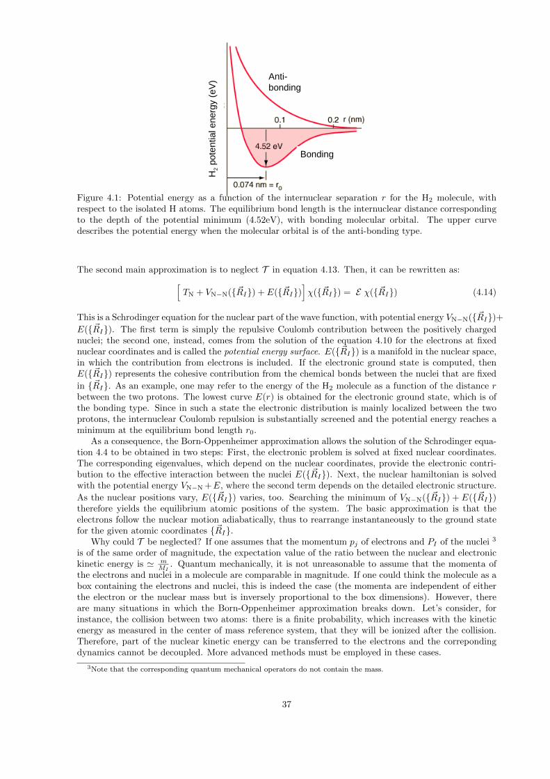
Bonding

Anti-bonding

H2

pote

nti a

l ene

rgy

(eV

)

Figure 4.1: Potential energy as a function of the internuclear separation r for the H2 molecule, withrespect to the isolated H atoms. The equilibrium bond length is the internuclear distance correspondingto the depth of the potential minimum (4.52eV), with bonding molecular orbital. The upper curvedescribes the potential energy when the molecular orbital is of the anti-bonding type.

The second main approximation is to neglect T in equation 4.13. Then, it can be rewritten as:[TN + VN−N(~RI) + E(~RI)

]χ(~RI) = E χ(~RI) (4.14)

This is a Schrodinger equation for the nuclear part of the wave function, with potential energy VN−N(~RI)+E(~RI). The first term is simply the repulsive Coulomb contribution between the positively chargednuclei; the second one, instead, comes from the solution of the equation 4.10 for the electrons at fixednuclear coordinates and is called the potential energy surface. E(~RI) is a manifold in the nuclear space,in which the contribution from electrons is included. If the electronic ground state is computed, thenE(~RI) represents the cohesive contribution from the chemical bonds between the nuclei that are fixed

in ~RI. As an example, one may refer to the energy of the H2 molecule as a function of the distance rbetween the two protons. The lowest curve E(r) is obtained for the electronic ground state, which is ofthe bonding type. Since in such a state the electronic distribution is mainly localized between the twoprotons, the internuclear Coulomb repulsion is substantially screened and the potential energy reaches aminimum at the equilibrium bond length r0.

As a consequence, the Born-Oppenheimer approximation allows the solution of the Schrodinger equa-tion 4.4 to be obtained in two steps: First, the electronic problem is solved at fixed nuclear coordinates.The corresponding eigenvalues, which depend on the nuclear coordinates, provide the electronic contri-bution to the effective interaction between the nuclei E(~RI). Next, the nuclear hamiltonian is solvedwith the potential energy VN−N +E, where the second term depends on the detailed electronic structure.

As the nuclear positions vary, E(~RI) varies, too. Searching the minimum of VN−N(~RI) + E(~RI)therefore yields the equilibrium atomic positions of the system. The basic approximation is that theelectrons follow the nuclear motion adiabatically, thus to rearrange instantaneously to the ground statefor the given atomic coordinates ~RI.

Why could T be neglected? If one assumes that the momentum pj of electrons and PI of the nuclei 3

is of the same order of magnitude, the expectation value of the ratio between the nuclear and electronickinetic energy is ' m

MI. Quantum mechanically, it is not unreasonable to assume that the momenta of

the electrons and nuclei in a molecule are comparable in magnitude. If one could think the molecule as abox containing the electrons and nuclei, this is indeed the case (the momenta are independent of eitherthe electron or the nuclear mass but is inversely proportional to the box dimensions). However, thereare many situations in which the Born-Oppenheimer approximation breaks down. Let’s consider, forinstance, the collision between two atoms: there is a finite probability, which increases with the kineticenergy as measured in the center of mass reference system, that they will be ionized after the collision.Therefore, part of the nuclear kinetic energy can be transferred to the electrons and the correpondingdynamics cannot be decoupled. More advanced methods must be employed in these cases.

3Note that the corresponding quantum mechanical operators do not contain the mass.

37

The Hellmann-Feynman theorem in DFT and the atomic forces. The atomic forces are thederivatives of the potential energy VN−N(~RI) + E(~RI) with respect to the atomic positions ~RI:~FI = −∇I

[VN−N(~RI) + E(~RI)

]. However, such a definition would imply to solve equation 4.11 and

obtain the eigenvalue E as well as its explicit dependence on the nuclear coordinates ~RI. Even if we use

finite-difference approximations for E(~RI), the calculations would be unfeasible for systems consisting

of more than a few atoms, since many Kohn-Sham equations with varying ~RI should be solved.Instead, we proceed differently and use the variational properties of the DFT. Consider the total

energy of the system of nuclei and electrons, with all of the nuclei fixed:

VN−N(~RI) + E(~RI)[n] (4.15)

Here E(~RI)[n] is the electronic energy that is a functional of the electron density which, according to

the DFT, reaches its minimum for the correct ground state density n. It also depends on the nuclearcoordinates in a parametric way, as stated by the Born-Oppenheimer approximation. Therefore, theatomic force can be also defined as the total derivative of the previous expression with respect to thecoordinate ~RJ :

~FJ = −dVN−N

d~RJ− dE

d~RJ(4.16)

The total variation of E consists of two contribution, through the explicit dependence on the parameter~RJ , and the implicit dependence on the electron density, which also varies with ~RJ :

dE

d~RJ=

∂E

∂ ~RJ+

∫d3r

δE

δn(~r)

∂n(~r)

∂ ~RJ=

∂E

∂ ~RJ+

∫d3rµ

∂n(~r)

∂ ~RJ

=∂E

∂ ~RJ+ µ

∂

∂ ~RJ

∫d3r n(~r) =

∂E

∂ ~RJ(4.17)

where we have used equation 2.25 ad the fact that∫d3r n(~r) = N independently of ~RJ . Therefore,

the total derivative of the density energy functional with respect to a given nuclear coordinates simplycoincides with the partial derivative. This is a very important result: computing the partial derivativeis quite simple, since it implies to derive only the terms that have an explicit dependence on ~RJ . Thereis no need to determine the change of the electron density with respect to variations of the externalparameters! This is a quite general result, which is valid for any external parameter λ (such as thevolume, the intensity of a magnetic field, etc.) in any theory that is based on a variational principle, suchas the DFT and Hartree-Fock method.

From a practical point of view, the partial derivatives ∂E∂λ are usually computed at the same time as the

energy, for all the most common parameters λ such as the atomic positions and the volume. Consideringthe breakdown of the total electronic energy (equation 3.25, only the external potential depends on

the atomic coordinates explicitly. In all-electron methods, Vext(~r) = −∑I

ZIe2

|~r−~RI |. The atomic force is

therefore:

~FI = −∂Vext + ∂VN−N

∂ ~RI=

−ZIe2

∫d3r n(~r)

(~r − ~RI)

|~r − ~RI |3+∑J 6=I

ZJZIe2 (~RJ − ~RI)

|~RJ − ~RI |3(4.18)

Note that the correct force must be computed with the electron density at its ground state value. Whenusing a plane waves basis set in conjunction with pseudo-potentials, the expression is more involved butstill easy to be computed numerically. Calculating forces takes as much computer time as determiningthe total energy for a given density n(~r). The actual implementations obviously depend on the explicitrepresentation used, and will not be detailed here.

4.3 Second order

We have seen that the first order variation of the energy (E(n) in the expansion 4.3) does not depend onn(1) but only on the ground state electron distribution n(0). This result, which is the DFT analogous of

38

the Hellmann-Feynman theorem in quantum mechanics, is based on the variational character of the totalelectronic energy. Similarly, we can consider the expansion of the energy at any order in the perturbation.An extension of Hellmann-Feynman theorem, which is called the ”2n + 1 theorem”, holds, which statesthat E(2n+1) depends on the variations of the electron density at all orders up to n (20). In particular,the second order variation of the energy E(2) depends on both n(0) and n(1). The ground state density iscomputed through the Kohn-Sham equations 2.33 and 2.34. From the latter one, the first-order variationof the electron density is:

n(1) =∑j

fj ψ(1)j ψ

(0)∗j + C.C. (4.19)

ψ(1)j may be computed through the so called Sternheimer equation, which we derive in the following.

Consider the Schrodinger equation[H(0) +H(1) +H(2) + . . .)− (ε

(0)i − ε

(1)i − ε

(2)i + . . .)

](ψ

(0)i − ψ

(1)i − ψ

(2)i + . . .) = 0 (4.20)

where H(n) is known through all orders. We assume that it has been solved at zero order, so that we

know ε(0)i and ψ

(0)i , while ε

(1)i and ψ

(1)i must be determined. According to standard perturbation theory,

ε(1)i = 〈ψ(0)

i |H(1)|ψ(0)i 〉. In order to find ψ

(1)i , let’s consider the first-order terms in the Schrodinger

equation 4.20 (that is, we ignore all n-order terms with n > 1 as well products between first-order terms):[H(0) − ε(0)

i

]ψ

(1)i =

[H(1) − ε(1)

i

]ψ

(0)i (4.21)

This is the Sternheimer equation. When the hamiltonian and the Kohn-Sham orbitals is discretized

on a basis set, the equation 4.21 is of the form A~x = ~b, with A = H(0) − ε(0)i I, ~x = ψ

(1)i and ~b =[

H(1) − ε(1)i

]ψ

(0)i . Its solution is: ~x = A−1~b, whenever A−1 exists. When a plane wave basis set is used,

A is a large matrix (consisting of up to ∼ 105 elements), so that its inversion is cumbersome. However,it can be obtained by iterative processes that imply only matrix - vector multiplication without the needof computing A−1 by direct inversion.

Atomic vibrations. We assume that the Born-Oppenheimer separation holds and that the electronand nuclear dynamics can be decoupled. In equation 4.14, the potential energy term for the nuclear motionis Epot(~RI) = VN−N(~RI) + E(~RI), where the last term represents the effective contribution byelectrons relative to the fixed nuclei. We also make the assumption that the nuclei can be considered asclassical particles, which is reasonable apart from light elements such as H or He. In order to find thesmall oscillations of the system, we expand the potential energy in terms of the nuclear displacements

~uI = ~RI − ~R(0)I from the equilibrium positions ~R

(0)I :

Epot(~RI) = Epot(~R(0)I ) +

∑I,α

[∂Epot

∂RI,α

]0

uI,α +∑

I,α;J,β

1

2

[∂2Epot

∂RI,α∂RJ,β

]0

uI,αuJ,β + . . . (4.22)

where I and J runs on the atoms and α, β = 1, 3 label the cartesian components. The first order

term is null, since at equilibrium[∂Epot

∂RI,α

]0

= 0. Within the harmonic approximation, we neglect in the

expansion 4.22 all terms beyond the second order in the atomic displacements, that we suppose to besmall. Therefore, the atomic force on the atom I that is due to the set of displacements is proportionalto the atomic displacements uJ,β 4:

FI,α = −∑J,β

CI,α;J,βuJ,β (4.23)

where we have introduced the (3Nat × 3Nat) interatomic force constant matrix:

CI,α;J,β =

[∂2Epot

∂RI,α∂RJ,β

]0

(4.24)

4This is quite usual: we speak of linear response theory whenever we neglect terms beyond second order in the expansionof the energy as a function of the perturbations. This apparent semantic contradiction is due to the fact that the generalizedforces are indeed linear in the perturbation!

39

It can be shown that the force constant matrix is symmetric (CI,α;J,β = CJ,β;I,α) and that the sum of itselements along any row is zero (

∑J,β CI,α;J,β = 0).

By considering the nuclei as classical particles, their motion is governed by the Newton equation:

MId2uI,αdt2

= FI,α = −∑J,β

CI,α;J,βuJ,β (4.25)

We look an oscillatory solution with frequency ω/2π of the form:

uI,α(t) =u

(0)I,α√MI

eiωt (4.26)

By using this expression in the equation of motion 4.25, we obtain the linear homogeneous system in the

unknown amplitudes u(0)J,β : ∑

J,β

[CI,α;J,β√MIMJ

− ω2δIJδαβ

]u

(0)J,β eiωt = 0 (4.27)

which has non trivial solutions (u(0)J,β 6= 0) only if the determinant of the coefficients is null:

Det

[CI,α;J,β√MIMJ

− ω2I

]= 0 (4.28)

From the secular equation above, the frequencies ω2 are computed. Since the matrix CI,α;J,β/√MIMJ is

symmetric, the 3Nat solutions ω2k ≥ 0 with k = 1, 3Nat. From the corresponding normalized eigenvectors

xi,k, the amplitudes for the mode k on each atom I and cartesian component α can be determined as

u(0)i ∼

xi,k√MI

5.

Once the matrix of the interatomic force constants is known, the vibrational frequencies (the eigenval-ues) and the amplitudes for each atom (the eigenvectors) are thus obtained by standard diagonalizationtechniques. Therefore, the main problem is to compute CI,α;J,β/

√MIMJ . In practice, the perturba-

tions consist of small atomic displacements. Once the equilibrium geometry is found, the atoms can bedisplaced ”by hands” one by one, along the cartesian directions, in order to find the elements of theinteratomic force constant matrix by finite differences (for instance, by computing the variations of theatomic forces that are due to the displacements). This method is known as the frozen phonon calculation.It usually gives very good results in finite systems, such as molecules and clusters, provided that forcederivatives are well approximated by finite differences. The atomic displacements should be small enough

not to include anharmonic contributions (i.e. forces must be linear in u(0)I,α) and large enough in order to

avoid numerical errors (the finite difference F (x+dx)F (x−dx)2 dx → 0

0 if dx→ 0).

Periodic crystals: phonons. The case of crystal implies some additional complications. In a periodicsolid, the matrix of interatomic force constant depends only on the mutual distances between the atoms:displacing the origin of coordinates from a point to another one that is equivalent by lattice vectorstranslations produces no physical changes. Such property implies that the atomic displacements withindifferent unit cells of the crystal are related by:

u(0)n,I,α = u

(0)m,I,α ei

~k·~Ln−m (4.29)

where ~Ln−m is a direct lattice vector going from cell m to cell n and ~k a wave vector within the Brillouinzone. The previous expression is similar to that of one-electron orbitals in a periodic potential. Indeed,the Bloch theorem holds for the atomic vibrations in a periodic crystal, too, from which Equation 4.29can be derived. Accordingly, the number of independent vibrational degrees of freedom in a solid is given

by 3N(0)at , which is the number of atoms within the unit cell by the three spatial dimensions. By using

equation 4.29, all the vibrational properties can be determined by looking to a single unit cell, in principle.As in the case of the single-particle electronic orbitals, it is much better to work in the reciprocal space.

5Here, for the sake of conciseness, the indexes run on both cartesian and atomic labels (i = I, α)

40

Therefore, we introduce the dynamical matrix, which is the Fourier transform of the interatomic forceconstant matrix:

DI,α;J,β(~q) =∑~L

CI,0,α;J,~L,β ei~L·~q (4.30)

where the cell at the origin (0) is related to another one by the lattice vector ~L. The eigenvalues of

DI,α;J,β(~q) at any wave vector within the Brillouin zone yield 3N(0)at values of the squared frequencies

ω2(~q). The ω versus ~q plot is the phonon dispersion relation, which should be known for the wholeBrillouin zone, in principle.

If one uses periodic boundary conditions, each atomic displacement is periodically repeated in space,which poses practical restrictions on the phonon wave length (see exercise 1). Therefore, any calculationthat is based on the frozen phonon technique can only give phonons for a few ~q vectors in the Brillouinzone. For the case of phonon calculation in a solid, the perturbation is instead the variation of theexternal potential when the nuclei in ~RI are subject to the displacements ~uI :

∆Vext =∑I

Vext(~r − (~RI + ~uI))− Vext(~r − ~RI) (4.31)

with ~uI = λ ~eI cos(~q · ~RI) (4.32)

where λ is a small parameter, ~eI the phonon polarisation and ~q the phonon wave vector.In practice, the calculation of the vibrational properties of a molecule or a solid is performed in the

following way:

1. Find the equilibrium geometry and the corresponding electronic ground state, that is, the Kohn-

Sham orbitals ψ(0)i and the electron density n(0).

2. For each perturbation of the type illustrated in equations 4.31 and 4.32, compute the first-order

variations ψ(1)i and n(1). The Sternheimer equation can be used, or alternative approaches that

are not detailed here.

3. From ψ(0)i , ψ

(1)i , n(0) and n(1), compute the energy variations E(2) at the second order in the

phonon perturbation. Then, rely E(2) with the parameter of the perturbation (equations 4.31 and4.32) and construct the dynamical matrix. Its diagonalization yields the phonon energy ω(~q) andthe corresponding eigenvectors.

4. For a molecule, only the calculation at ~q = 0 is meaningful. For a periodic solid, at variance, repeatsteps 2 and 3 for selected wave vectors ~q within the Brillouin zone, in order to determine the phonondispersion relation.

Exercises

1. Consider a periodic chain of atoms with two distinct atoms per unit cell. Be L the length ofthe unit cell and M their number (M >> 1). Write the atomic displacements along the chainaccording to equation 4.28. Suppose now to change by hands the coordinate of an atom withinthe unit cell and apply the periodic boundary conditions. Which wave vector q does correspondto such perturbation? Imagine now to choose as unit cell the double of the primitive ones. Suchnew unit cell has length 2L and contains four atoms. Firstly, establish a correspondence betweenthe reciprocal lattice vectors of the primitive and the new unit cells. Then, change by hands thecoordinate of an atom within the unit cell and apply the periodic boundary conditions. Whichwave vector q corresponds to such a perturbation, in the coordinates of the new unit cell of size 2L?Which wave vector q corresponds to such a perturbation, in the coordinates of the (old) primitivecell of size L? Discuss a method to obtain the vibrational frequencies at q = π

mL by displacingatoms by hands and choosing unit cells of increasing lengths mL.

41

Bibliography

[1] N. Metropolis and S. Ulam, “The Monte Carlo method”, J. Amer. Stat. Ass. 44, 335 (1949).

[2] N. Metropolis et al., “Equation of state by fast computing machines”, J. Chem. Phys. 21, 1087(1953).

[3] B.J. Alder and T.E. Wainwright, “Studies in Molecular dynamics: general method”, J. Chem.Phys. 31, 459 (1959)

[4] R. Car and M. Parrinello, “Unified approach for molecular dynamics and density functional the-ory”, Phys. Rev. Lett. 55, 2471 (1985).

[5] P. Hohemberg and W. Kohn, “Inhomogeneous electron gas”, Phys. Rev. 136, B864 (1964).

[6] W. Kohn and L.J. Sham, “Self-consistent equations including exchange and correlation effects”,Phys. Rev. A140, 1133 (1965).

[7] T. Kato, Commun. Pure Appl. Math. 10, 151 (1957).

[8] R.G. Parr and W. Yang, “Density Functional Theory of Atoms and Molecule”, Oxford Univ. Press(1989); R.M. Dreizler and E.K.U. Gross, “Density Functional Theory”, Springer-Verlag (1990).

[9] R.M. Martin, “Electronic Structure: Basic Theory and Practical Methods”, Cambridge Univ.Press (2004).

[10] F. Finocchi, J. Goniakowski, X. Gonze, and C. Pisani, ”An introduction to First-Principles sim-ulations of extended systems”, in Handbook of Numerical Analysis, vol.X (special volume onComputational Chemistry), edited by C. Le Bris, pages 377-451 (Elsevier, Amsterdam, 2003).

[11] G.D. Mahan and K.R. Subbaswamy, “Local Density Theory of Polarizability”, Plenum Press(1990).

[12] N.W. Ashcroft and N.D. Mermin, “Solid State Physics”, Holt-Saunders (1981).

[13] F. Bassani and G. Pastori Parravicini, “Electronic states and optical transitions in solids”, Perg-amon Press (1975).

[14] D.J. Chadi and M.L. Cohen, “Special Points in Brillouin Zone”, Phys. Rev. B 8, 5747 (1973)

[15] H.J. Monkhorst and J.D. Pack, “Special points for Brillouin-zone integrations”, Phys. Rev. B 13,5188 (1976).

[16] M. Verstraete and X. Gonze, Comp. Mater. Sci. 30, 27 (2004).

[17] M.C. Payne, M.P. Teter, D.C. Allan, T.A. Arias and J.D. Joannopoulos, “Iterative Minimizationtechniques for ab initio total energy calculations - Molecular Dynamics and Conjugate Gradients”,Rev. Mod. Phys. 64, 1045 (1992).

[18] P. Pulay, Chem. Phys. Lett. 73, 393 (1980).

[19] S. Baroni, S. De Gironcoli, S. Dal Corso et al, “Phonons and related crystal properties fromdensity functional perturbation theory”, Rev. Mod. Phys. 73, 515 (2001)

[20] X. Gonze, “Perturbation expansion of variational principles at arbitrary order”, Phys. Rev. A 52,1086 (1995).

42