DEPARTAMENTO DE ECONOMIAPUC-RIO

TEXTO PARA DISCUSSÃONo. 399

MONETARY POLICY IN THE AFTERMATHOF CURRENCY CRISIS: THE CASE OF ASIA1

Ilan GoldfajnPUC/Rio

Taimur BaigUniversity of Illinois at Urbana-Chamapaign

1 The authors thank Bijan Aghevli, Andrew Berg, Debra Glassman, Jonathan D. Ostry, David Goldsbrough,

Poonam Gupta, Wanda Tseng, Prakash Loungani, Kanitta Meesook, Mark Stone, Jeromin Zettelmeyer, andseminar participants and reviewers at the International Monetary Fund and at the University of Washington atSeattle.

2

JEL Classification Numbers: E44, E63

Keywords: Monetary policy, interest rates, inflation

Abstract

This paper evaluates monetary policy and its relationship with the exchange rate in

the five Asian crisis countries. The findings are compared to previous currency

crises in recent history. The paper finds that there is no evidence of overly tight

monetary policy in the Asian crisis countries in 1997 and early 1998. There is also

no evidence that high interest rates led to weaker exchange rates. The usual trade-

off between inflation and output when raising interest rates suggested the need for

a softer monetary policy in the crisis countries to combat recession. However, in

some countries, corporate balance sheet considerations suggested the need to

reverse overly depreciated currencies through firmer monetary policy.

3

I. INTRODUCTION

What is the appropriate monetary policy in the aftermath of a currency crisis?

Should interest rates be raised to appreciate the currency? The Asian crisis has put

these questions at the center of economic policy making. This paper attempts to

shed light on this question by analyzing a few episodes of large currency

depreciation in the aftermath of currency crises, in particular the Asian crisis cases.

The paper intentionally does not aim to study the general relationship

between exchange rates and interest rates. This leaves out several interesting issues

but allows the paper to concentrate on the role of monetary policy in reestablishing

currency stability after a large collapse.

The analysis of the appropriate monetary policy in the aftermath of currency

crises has four building blocks. The first is to evaluate whether the exchange rate

has overshot during the crisis, or in other words, whether the real exchange rate

(RER) has become undervalued and needs to be brought back to equilibrium. The

second block is to identify the mechanisms through which the RER could be

corrected in case it is undervalued (or maintained in case the new level is deemed

appropriate). There are two ways to reverse an undervaluation --through nominal

currency appreciation or through higher inflation at home than abroad (or a

combination of the two). If avoiding an inflation buildup is an important concern

and/or nominal appreciation is desirable for the benefit of domestic corporate and

bank balance sheets, the extent to which the reversal occurs through nominal

appreciations is fundamental. A key factor in evaluating the likelihood of this

reversal is to estimate the exchange rate passthrough in the economy --or in other

4

words, the extent to which the correction is expected to occur through inflation in

the economy, in the absence of major changes in policies. The third block is to

identify through which policies and under what circumstances the reversal occurs

through nominal appreciation. In particular, it is important to evaluate whether

nominal appreciations occurs mainly in cases where interest rates are kept high. In

addition, it is also important to evaluate whether other economic conditions, for

example the state of the banking system and corporate sector, influence the

relationship between interest and exchange rates. Finally, the fourth block is to

evaluate the desirability of raising interest rates. Even if one identifies a set of

policies and conditions that maximizes the effect of interest rates on the exchange

rate, the costs of raising interest rates in terms of output loss, unemployment, and

financial system fragility could outweigh the benefits of a more appreciated nominal

exchange rate.

There is considerable debate on each the four building blocks in general, and

for the case of Asia in particular. The debate on the right measure of

undervaluation (or overvaluation) has always been controversial, with some even

doubting the notion that a currency could be fundamentally out of line. In the case

of Asia, there is doubt whether the currencies were overvalued before the crisis and

whether, despite the large real depreciation that followed the crisis, the currencies

became undervalued (some argue that the extent of the shock justifies a much lower

real exchange rate). With respect to the extent of exchange rate passthrough, initial

estimates suggest that the Asian economies have a much lower passthrough than

typical developing countries, which implies that the real depreciation has persisted

for longer than in other crisis cases, but also implies that the correction of the RER

5

would likely occur through nominal appreciations (unless the current passthrough

estimates reflect longer lags in Asia and we will observe much higher inflation in the

future) .

An important debate has been about the relationship between interest rates

and exchange rates. The traditional approach stresses that tight monetary policy is

necessary to support the exchange rate and curb inflationary pressures. In the short

run, higher interest rates make speculation more expensive by increasing the cost

of shorting the domestic currency. Also, higher interest rates increase the return

that an investor obtains from investing in the country. In the long run, higher

interest rates may affect the exchange rate by reducing absorption and improving

the current account. However, in the discussion of the role of monetary policy in

the Asian crisis, several economists have raised the possibility that an increase in

interest rates would have a negative effect on the exchange rate. Jeffrey Sachs

(1998, pg. 31), for example, has been vocal in expressing his views that high

interest rates would not stabilize currencies in the Asian case:

“Despite sharply higher interest rates, currencies have not appreciatedso the supposed benefits of this policy are in question. It is entirelypossible that in the unique conditions of the midst of a financial panic,raising interest rates could have the perverse effect of weakening thecurrency . . . Creditors understood that highly leveraged borrowerscould quickly be pushed to insolvency as a result of several months ofhigh interest rates. Moreover many kinds of interest-sensitive marketparticipants, such as bond traders, are simply not active in Asia’s limitedfinancial markets. The key participants were the existing holders ofshort term debt, and the important question was whether they would ornot roll over their claims. High interest rates did not feed directly intothese existing claims (which were generally floating interest rate notesbased on a fixed premium over LIBOR). It is possible, however, that byundermining the profitability of their corporate customers, higherinterest rates discouraged foreign investors from rolling over theirloans.”

6

On the opposite side of this debate Krugman (1998) writes:

“I have heard some people propose what amounts to a sort of foreignexchange- interest rate Laffer curve: if you cut interest rates this willstrengthen the economy, and the currency will actually rise. This is assilly as it sounds.”

The precedence of the debate on the relationship between exchange rates and

interest rates over the debate on the optimality of monetary policy in crisis cases is

raised by Stiglitz (1998), a critic of the traditional approach:

“Thus, although countries confronted with an exchange rate crisis havesometimes viewed themselves as facing a tradeoff between the adverseeffect of exchange rate depreciation and interest rate increases, ifincreases in interest rates lead to a decreased capital flow, there is notradeoff: higher interest rates weaken the economy directly, and actuallyexacerbate the decline in the exchange rate.”

The other big debate on the role of monetary policy is on the desirability of

increasing interest rates to support the exchange rate. Some doubt the optimality

of tight policies. This line of argument takes as given that high interest rates may

eventually stabilize the exchange rate but argue that the costs of doing so are very

high and that letting the exchange rate float freely (and possibly become more

undervalued for a while) is the least costly option. The costs of a tight monetary

policy are usually identified with a large recession, unemployment, financial system

bankruptcies, credit crunch and corporate failures. Of course, there are also costs

in letting the exchange rate depreciate further, as argued by Goldstein (1998):

“When market participants lose confidence in a currency and attach ahigh probability to further falls, it is difficult to induce them to hold thecurrency without higher interest rates...Moreover, halting a free fall ofthe currency takes on added importance when banks or corporations inthe crisis country have large foreign currency obligations coming due inthe short term.”

7

This paper is organized as follows. In section II.A., the issue of the extent

of undervaluation in Asia and other cases is explored. In section II.B., the paper

analyzes the exchange rate passthrough in the Asian crisis case so far and compares

it with other cases in history. In addition, it calculates the probability that a

reversion of an undervaluation could occur through nominal appreciation. In

section III, the paper explores the link between exchange rates and interest rates in

the aftermath of the Asian crises. In section IV, the tradeoffs involved in the

decision to raise interest rates are analyzed.

II. OVERSHOOTING AND REVERSALS

The effectiveness and desirability of implementing tight monetary policies to

stabilize a currency crisis depends to a certain extent on the underlying causes of

the crisis. A fair amount of attention has been dedicated to the question of what

caused the Asian crises. There are three broad explanations:

(i) BOP crises driven by traditional fundamentals (à la Krugman 1978,

Flood and Garber (1984)): overvaluation of the RER coupled with too much credit

expansion resulting in excess demand and a growing balance of payments deficit

that culminates in crisis and the adjustment of the RER.

(ii) Crisis as a result of panic by investors (Sachs and Radelet (1998)).

Asian currency crises must be understood as a run on international reserves, i.e.,

as the international equivalent of commercial bank runs. Countries were vulnerable

to runs because of high ratios of short term debt to reserves.

(iii) Crises were driven by more sophisticated fundamentals and should be

understood as financial crises rather than simply currency crises (Krugman, 1998).

The financial crises were caused by overlending to risky and unproductive projects

8

fueled by explicit and implicit guarantees. When the bubble burst the crisis

occurred.

There is also the possibility of a combination of the explanations above. For

example, one may advance the argument that fundamental reasons made the

countries vulnerable to speculative attacks and that panic was an element of the

crises but not their ultimate cause.

Tight monetary policy is less controversial if one believes the underlying

cause for the crises is point (i) above. Increases in domestic interest rates serve

simultaneously to increase the interest rate differential with respect to the rest of

the world and reduce the level of activity in the economy. In contrast, the panic and

financial crisis explanations are not an overheating story and, therefore, there is a

possible trade off for policy makers between recession (or the health of the banking

system) and currency stabilization.

In general, it would be futile to try to appreciate the currency if one believed

the currency has not overshot. Therefore, the following section evaluates the

equilibrium real exchange rates for both the Asian and some other currency crises

cases.

A. Is there Overshooting?

Table 1 shows available estimates of RER overvaluation prior to the Asian

crises (Indonesia, Korea, Malaysia, Philippines and Thailand) and to 5 other crisis

cases (Mexico(1982), Chile (1982), Mexico(1994), Sweden (1992) and UK (1992)).

9

The overvaluation estimates for the five Asian countries are taken from the

literature. Goldman Sachs uses the Dynamic Equilibrium Emerging Markets

Exchange Rates model (GSDEEMER) to calculate the equilibrium value for a large

set of countries. For each country, they find a cointegrating relation between the

multilateral real exchange rate and a set of fundamentals (using leads and lags)

using quarterly data since 1980. The relationship between the real exchange rate

and the fundamentals is interpreted as a long term relationship and its predicted

value the equilibrium exchange rate. The fundamentals include a large set of

variables that are known to influence the equilibrium real exchange rate --including

terms of trade, openness, government size, and capital flows. The exact set of

fundamentals varies per country. The difference between the equilibrium value and

the actual exchange rate is defined as a misalignment measure

(overvaluation/undervaluation). Chinn (1998) uses the Purchasing Power Parity

concept to evaluate whether seven East Asian currencies were overvalued before

the crisis. He uses a simple model that uses deviations from PPP and a trend in the

real exchange rate to define misalignment. For the other crisis cases, the

overvaluation measures were derived in Goldfajn and Valdés (1996) using a

methodology similar to Goldman Sachs’ methodology.

10

The existence of large overvaluations would imply that one should expect

large corrections of the RER in the aftermath of the crisis and would not necessarily

call for policy action. The Latin-American crisis cases had clear misalignment in

their RER of the order of 20-25 percent prior to the crisis. In contrast, the

European cases had only mild overvaluations. Few observers indicated at the time

of the ERM crises that overvaluation was at the root of the crisis. In fact, several

papers advanced the hypothesis that the 1992 European crises were of the self-

fulfilling nature (the so-called second generation models).2

In Asia, the different estimates indicate that Malaysia, Philippines and

Thailand systematically appear to have had the most overvalued currencies while

Korea and Indonesia the least overvalued (Chinn’s estimate indicates that the Won

was actually undervalued). The magnitude of the subsequent real devaluations were

not correlated with the initial overvaluation measures. In fact, besides Thailand, the

larger depreciations occurred precisely in Indonesia and Korea. In all the Asian

cases the extent of the real devaluation was larger than the initial overvaluation.

One could argue that the previous overvaluation estimates are not reliable or,

alternatively, that the crisis altered significantly the equilibrium RER’s such that a

larger depreciation of the RER is justified.3 In fact, some argue that the large terms

of trade decline in Korea justifies a large equilibrium depreciation after the crisis.

However, the results suggest that there was scope to believe that the currencies had

overshot or, at least, that further declines in the exchange rate were not desirable.

2 See Eichengreen, Rose and Wyplosz (1994).

3 The argument that the equilibrium RER had significantly depreciated must rely on permanent rather thantransitory changes in fundamentals. For example, a post crisis panic by foreign investors that reduces theavailable short-term capital to the economy should not be confused with a permanent reduction in the capitalavailable to the economy that would require an equilibrium depreciation.

11

B. RER Reversion and Exchange Rate Passthrough

There are two ways to reverse an undervaluation through nominal currency

appreciation or through higher inflation at home than abroad (or a combination of

the two). If avoiding an inflation build up is an important concern and/or nominal

appreciation is desirable for the benefit of domestic corporate and bank balance

sheets, the extent to which the reversals occurs through nominal appreciations is

fundamental. A key factor in evaluating the likelihood of this reversion is to

estimate the exchange rate passthrough in the economy.

Table 2 shows nominal depreciations, inflation and exchange rate

passthrough coefficients for the 10 episodes. It is evident that the Latin American

cases are different. They had larger depreciations, higher inflations, and larger

passthrough coefficients (in the order of 0.4) than the European and Asian cases.

The European cases had depreciation rates of about 30-50 percent but only single

digit inflations in the first 12 months after the crisis implying very low passthrough

coefficients. The Asian crises are an intermediate case between the European and

Latin American cases both in terms of inflation and passthrough coefficients.

It is interesting to note that the reversal of the real exchange rate occurred

more slowly in the European cases. Inflation rates were higher in the second year

after the crisis; the passthrough coefficients doubled or tripled when looking instead

over the first 24 months. This suggests that if the Asian crisis cases follow the

European pattern of slower but longer adjustment of RER’s there is a potential role

for policies to avoid inflationary reversals. (Of course, what determines the extent

of the passthrough is not only the effectiveness of short run policies but also the

inflationary history and labor market institutions of the country in question.)

12

In a more systematic way, we analyze all the episodes of currency collapses

that resulted in undervaluations greater than 15 percent from a sample of 80

countries between 1980-1998.4 We defined the undervaluation series as deviations

of the actual exchange rate from a Hodrick-Prescott filtered series. The filtered

series captures stochastic trends in the series and allows us to concentrate on the

cyclical behavior of potentially non-stationary RER series. The filtered series

represents the predicted equilibrium RER and captures the permanent changes in the

relative prices between countries while the estimated undervaluation series

represents the cyclical component of the RER movements since, as a misalignment,

it must eventually correct itself. This approach will also net out from the

undervaluation measure trends in the equilibrium RER, as for example the Balassa-

Samuelson effect.5 We used the INS effective real exchange rate that should, in

principle, take into account third country effects.

Table 3 shows the number of cases found for different degrees of

undervaluations. Since 1980, there are 116 cases with undervaluations of more than

10 percent but only 28 with more than 30 percent. Table 4 shows that the average

duration of the episodes is 30 months with the overshooting reversing slowly over

a period of about 20 months. This suggests that the reversal of undervaluation in

Asian may be drawn out. This is an important consideration since there may be a

role for policies to reduce the duration of the process even if the reversal occurs

through nominal appreciations.

4 This analysis is drawn from the paper entitled “Does tight monetary policy stabilize the exchange rate? ” by

Goldfajn and Gupta (1998).

5 The Balassa-Samuelson effect occurs when a country's tradable sector productivity grows faster than that ofits trading partners ones and this differential growth is smaller in the non-tradable sector. Then the relative priceof non-tradables increases faster at home than abroad, leading to a domestic real appreciation.

13

We calculate the probability of reversing an undervaluation through

appreciations of the nominal exchange rate rather than higher inflation. We define

that a reversal is through nominal appreciation if the exchange rate is responsible

for more than 50 percent of the reversal.6 The results show that the probability of

a reversal through nominal appreciation is less than 40 percent (see Chart 1).

6 For stricter definitions of reversals, i.e. requiring the exchange rate to undo up to 90 percent of the

overshooting, we obtain much lower probabilities. See Goldfajn and Gupta (1998).

(in percent, + overvaluation)

Overvaluation Chinn (1998) Overvaluation Goldman Sachs (1998) Goldfajn and Valdes (1996) Real DepreciationMay, 1997 1/ June, 1997 2/ Month Prior to Crisis 12 Month After Crisis 3/

Thailand 7,0 3,9 26,0Malaysia 7,9 4,4 25,2Philippines 19,1 5,5 22,1Indonesia -5,5 1,2 68,2Korea -9,1 3,3 26,5

Chile (82) 17,7 19,9Mexico (82) 25,6 43,8Mexico (94) 22,6 27,8Sweden (92) 9,7 20,1UK (92) 4,6 11,1

1/ PPI -based calculation.

2/ Based on J.P.Morgan Database.

3/ Based on REER from June 97 - June 98 in Asian cases.

Table 1: RER Overvaluation Measures and Real Depreciations for Selected Crisis Cases

14

Depreciation Cutoff Total (percentage) # of Cases w/Tight Policy 1/ w/ Banking Crises 2/

10 116 32,3 41,415 77 29,2 45,420 49 22,5 46,925 36 17,2 50,030 28 13,6 57,1

Source: Goldfajn and Gupta (1998).1/ Tight Policy is defined as real rates higher in the period than average rates.

2/ Banking crises dummies are obtained from several sources. See above source.

Phase Average # of Months

Build Up 9,5Reversal 20,4

Total 29,9Source: Goldfajn and Gupta (1998).

Table 3. Number of Undervaluation Cases

Table 4. Duration of Undervaluation Cases

Proportion of Cases

CPI Inflation 1/ Depreciation 1/ 2/ Passthrough Coefficient 3/ Passthrough Coefficient 3/(After 1 year) (After 2 years)

Asia:Thailand 10,8 47,7 0,23Malaysia 6,3 39,3 0,16Philippines 9,9 38,8 0,26Indonesia 59,6 394,4 0,15Korea 6,7 35,3 0,19Other Cases:Chile (82) 31,2 92,6 0,34 0,43Mexico (82) 108,3 269,6 0,40 0,40Mexico (94) 48,5 122,5 0,40 0,40Sweden (92) 4,8 52,3 0,09 0,16UK (92) 1,7 32,4 0,05 0,14

1/ First 12 months of the crisis. For Korea based on Sept, 97 to July, 98.

2/ Based on NEER for Asian countries and bilateral rates with respect to the dollar in the other cases.

3/ CPI inflation divided by depreciaton.

Table 2: Inflation, Depreciation and Passthrough Coefficients for Selected Crisis Cases

15

III. RELATIONSHIP BETWEEN INTEREST RATES AND EXCHANGE RATES

A. Theoretical Considerations

The conventional wisdom is that monetary policy tightens liquidity and

stabilizes the exchange rate. In the short run, higher interest rates makes speculation

more expensive. Also, higher interest rates increase the return that an investor

obtains from investing in the country. In the long run, higher interest rates may

affect the exchange rate by reducing absorption and improving the current account.

In the midst of an exchange rate crisis, interest rates are raised to make speculation

against the currency more costly. If borrowing (shorting) the domestic currency to

invest in the foreign currency is allowed, raising interest rates directly increases the

costs of speculation. Even if shorting the domestic currency is not allowed, the

increase in interest rates affects the opportunity cost of an investor deciding

whether to invest in the domestic economy.

The expected return in investing in the country depends on the promised

interest rate and the expected depreciation. The interest differential with respect

to the rest of the world should allow for both an exchange rate risk premia and a

probability of default:7

R+e]E[+i=E[i] * ∆

where E[∆e] is the expected depreciation, E[i] is the expected return of an

investment in the domestic economy, i* is the safe return on an equivalent

international asset and R is the risk premium that is demanded by risk averse foreign

7 Default here is defined more generally including partial payment, delay of payments or introduction of exchange

controls.

16

investors faced with exchange rate volatility.8 In principle, increases in interest

rates should increase the expected return, turning investing in the domestic

economy more attractive relative to abroad (i.e., making the right hand side of the

equation above larger than the left hand side) and inducing capital inflows, which

would increase the supply of dollars and immediately appreciate the exchange rate

up to the point where the equation above holds again (in the Dornbusch (1976)

model the exchange rate should actually overshoot its target such that agents expect

a future depreciation).

8 The risk premium must include also a portion for the uncertainty induced by default probability.

0,00

0,05

0,10

0,15

0,20

0,25

0,30

0,35

0,40

0,45

0,50

P

r

o

b

a

b

i

l

i

t

y

15 20 25 30 35

Degree of Undervaluation

Chart 1: Probability of Reversing Undervaluations through Nominal Appreciations

(Success is proportion > 50 percent)

17

However, interest increases may reduce the expected return by increasing the

probability of default.

Interest rates may affect the probability of default by increasing the borrowing costs

of corporations, by depressing the economy and reducing profits, by altering the net

worth of corporations adversely exposed to interest rate changes, or, finally, by

affecting the health of the banking system that tends to be naturally exposed to

interest rate changes. The latter have a compounding effect on the economy since

problems in the banking system may lead to credit crunches, disintermediation and

bad allocation of credit.

Formally, the expected return on the domestic asset E[i] can be written as

the product of the domestic interest rate, i, times the probability of repayment, ρ:

E[i] = ρ (i) i. The equation can be rewritten in the following way:

Chart 2: Expected Returns and Interest Rates

Interest Rates (i)

Expected Return, E(i)= rho (i) i

i_d

18

R+e]E[+i = (i)i * ∆ρ

where r`<0, r``<0.

Therefore, even though one should expect increases in interest rates to

attract capital, there may be cases where additional increases in interest rates reduce

the expected return and generate capital outflows. In such cases, raising interest

rates paradoxically depreciates the currency (see Chart 2).

The level of interest rates needed to defend (or appreciate) a currency may

be substantial. For example, in order to defend an expectation of a one percent fall

in the exchange rate the next day, the overnight interest rate must be at least one

percent per day (which is 3,678 percent per annum).9 If agents are risk averse (and

there is a positive risk premium, R) and the default probability is large, the required

interest rate would be larger.

Proponents of tighter monetary policy argue that higher interest rates need

only be temporary. Once the exchange rate has been stabilized interest rates could

be allowed to decline. This argument is important given that the costs of

persistently high interest rates could be substantial.

However, the question then is why should a temporary increase in interest

rates lead to permanent effects on the exchange rate? One answer is that

temporarily tight policies may signal the determination of the monetary authority

to pursue exchange rate stability and low inflation. Temporary policies may then

change the beliefs of investors. Even when the tight policies are withdrawn, the

exchange rate would stabilize at a higher level.

9 This example is drawn from Stiglitz (1998).

19

Tight monetary policies do not always serve as a credible signaling device.

Drazen and Masson (1994) have shown that if the costs of implementing the tight

policies are too high, the temporary policy would actually reduce credibility because

investors know that the policy could not be sustained. Under this theory, the

relationship between interest rates and the exchange rate could be negative. When

there are doubts about the determination of the authorities and temporary increases

in interest rates lead to important reputational gains to the authorities, the effect of

raising interest rates should be positive. However, when the reputational arguments

are not essential and there are important structural problems, raising interest rates

may have the opposite effect.

B. Interest Rate Policy in the Asian Crises Episodes: 1997-98

This section analyzes interest rate policy in the aftermath of the five Asian

crises (Indonesia, Korea, Malaysia, Philippines and Thailand). There are several

issues to consider.

The first issue is what measures of the nominal interest rate better represents

the tightness of monetary policy and its effect on the exchange rate. Charts 3A and

3B show both inter-bank rates and “policy rates” for each of the crisis countries in

1996-98.10 The charts suggest that for most of the countries, the major movements

of monetary policy can be captured by any of the interest rates since they tend to

move together. In what follows we use the “policy rates” as our representative

nominal interest rate. The chart also shows the sharp increases in nominal interest

rates since the crisis. Most of the countries, however, seem to have waited to raise

10The �policy rates� are the 1 month repo rate for Thailand, the 91-day T-bill rate for Philippines, the 3-Month

Klibor for Malaysia, the 30-day JIBOR rate for Indonesia, and the overnight interbank rate for Korea.

20

interest rates until late in 1997 or early 1998. Indonesia initially raised interest rates

substantially in July - August 1997 but reduced them subsequently, only raising

them to higher levels in March - April 1998. Korea raised interest rates significantly

at the end of the year, after the crisis. Thailand increased nominal rates continuously

from May 1997 to March 1998.

The second issue is the appropriate expected inflation rate to be used in

calculating real interest rates. The approach taken here is to calculate several

measures of real interest rates based on different assumptions regarding expected

inflation. Chart 4 shows five measures of real interest rates for each country. The

measures

21

NOMINAL INTEREST RATES (in percent per annum)

Sources: Data provided by authorities; and IMF staff calculations

Chart: 3A

Hong Kong

2

4

6

8

10

12

J-96

M-96

M-96

J-96

S-96

N-96

J-97

M-97

M-97

J-97

S-97

N-97

J-98

2

4

6

8

10

12

3 month HIBOR

overnight interbank(ave.)

Korea

5

10

15

20

25

30

J-

96

M-

96

M-

96

J-

96

S-

96

N-

96

J-

97

M-

97

M-

97

J-

97

S-

97

N-

97

J-

98

M-

98

M-

98

5

10

15

20

25

30

overnight interbank(ave.)30 day interbank

Malaysia

5

6

7

8

9

10

11

12

J-96

M-96

M-96

J-96

S-96

N-96

J-97

M-97

M-97

J-97

S-97

N-97

J-98

M-98

M-98

5

6

7

8

9

10

11

12

overnightinterbank (ave.)3 monthKLIBOR30 dayinterbank

Indonesia

0

10

20

30

40

50

60

70

80

J-97 M-97 M-97 J-97 S-97 N-97 J-98 M-98 M-980

10

20

30

40

50

60

70

80

overnightJIBOR(ave.)

30 dayJIBOR

Thailand

5

10

15

20

25

30

J-97

F-97

M-97

A-97

M-97

J-97

J-97

A-97

S-97

O-97

N-97

D-97

J-98

F-98

M-98

A-98

M-98

5

10

15

20

25

30

overnight interbank(ave.)30 day interbank

1 month repo. rate

Philippines

5

10

15

20

25

30

35

J-96

M-96

M-96

J-96

S-96

N-96

J-97

M-97

M-97

J-97

S-97

N-97

J-98

M-98

M-98

5

10

15

20

25

30

35

overnight interbank(ave.)91 day T-bill

30 day interbank

22

OVERNIGHT CALL RATES (daily) (in percent per annum)

Source: Bloomberg

Chart: 3B

Indonesia

0

10

20

30

40

50

60

70

80

90

100

07/01/97 09/01/97 11/01/97 01/01/98 03/01/98 05/01/98

Korea

5

10

15

20

25

30

35

07/01/97 09/01/97 11/01/97 01/01/98 03/01/98 05/01/98

Malaysia

0

5

10

15

20

25

30

35

40

07/01/97 09/01/97 11/01/97 01/01/98 03/01/98 05/01/98

Philippines

0

20

40

60

80

100

120

07/01/97 09/01/97 11/01/97 01/01/98 03/01/98 05/01/98

Thailand

0

5

10

15

20

25

30

07/01/97 09/01/97 11/01/97 01/01/98 03/01/98 05/01/98

23

are based on expected inflation, which in turn is proxied by: (i) the following

month’s inflation p(t+1) annualized, (ii) survey forecasts from the Consensus

Forecasts, (iii) the quarterly moving-average inflation centered at t, (iv) the

previous month inflation p(t-1) annualized, and (v) the previous 12-month inflation.

The latter measures (iv)-(v) are based on adaptive expectations assumption, the

former ones (i)-(ii) are based on rational expectations assumptions (theoretically,

the survey forecasts should be based on all the information available) and measure

(iii) is a combination of the two assumptions. The main result is that for each

country there are two distinct groups of real interest rates with similar paths within

the group but differing substantially across them.

One group, shown in the lower panel of chart 4 for each country, is

composed by the real interest rates constructed using the past-12-month-inflation

rates and the one based on survey data, which, surprisingly, implies that the

forecasters in the survey probably based their forecast mainly on past information.

These rates are always positive throughout the crisis and its aftermath. Some

patterns emerge. Korea has the highest real rates of the five Asian countries in a

range of 10-20 percent during the period, followed by Thailand at around ten

percent. The rest of the countries exhibit relatively moderate rates, e.g. Malaysia

(2-6 percent) or Philippines (4-12).

24

The other group of real interest rates uses some combination of previous,

current or future inflation as the measure of inflationary expectations. This group

shows that Indonesia, Korea and Malaysia had negative real interest rates in early

1998 and Thailand had the same in the third quarter of 1997. This is probably the

consequence of the fact that inflation picked up very strongly and nominal interest

rates lagged behind. For Indonesia and Philippines real interest rates have not to

date reached their pre-crisis levels. The main conclusion is that there is little

evidence of tight monetary policies in the Asian crisis countries in 1997 and early

1998, based on real interest rates using forward looking measures of expected

inflation.

Chart: 4REAL INTEREST RATES (various measures)

i - π qtr. ave: ____ i - π( t): __ __ i - π( t+1 ):- - - -

INDONESIA KOREA MALAYSIA

i - π (past 12 months): ____ i - π (survey forecast): - - - -

INDONESIA KOREA MALAYSIA

Sources: Data provided by authorities; and IMF staff calculations. Inflation forecast obtained from Asian Consensus Forecast.

-10

0

10

20

30

40

50

J-97 M-97 M-97 J-97 S-97 N-97 J-98 M-98 M-98 J-98

-250

-200

-150

-100

-50

0

50

J-97 M-97 M-97 J-97 S-97 N-97 J-98 M-98 M-98 J-98

-20

-10

0

10

20

30

40

J-96

M-96

M-96

J-96

S-96

N-96

J-97

M-97

M-97

J-97

S-97

N-97

J-98

M-98

M-98

J-98

0

2

4

6

8

10

12

14

16

18

20

J-96

M-96

M-96

J-96

S-96

N-96

J-97

M-97

M-97

J-97

S-97

N-97

J-98

M-98

M-98

J-98

-6

-4

-2

0

2

4

6

8

10

12

J-96

M-96

M-96

J-96

S-96

N-96

J-97

M-97

M-97

J-97

S-97

N-97

J-98

M-98

0

2

4

6

8

A-96

J-96

A-96

O-96

D-96

F-97

A-97

J-97

A-97

O-97

D-97

F-98

A-98

J-98

25

The third issue is whether real rates are the appropriate measure to evaluate the

tightness of monetary policy. One of the arguments raised in the theoretical section is that

high interest rates stabilize currencies by increasing the attractiveness of the economy to

(foreign) investors. This means that one could look instead at

i - π qtr. ave: ____ i - π( t): __ __ i - π( t+1 ):- - - -

PHILIPPINES THAILAND HONG KONG

i - π (past 12 months): ____ i - π (survey forecast): - - - -

PHILIPPINES THAILAND HONG KONG

Sources: Data provided by authorities; and IMF staff calculations. Inflation forecast obtained from Asian Consensus Forecast.

-10

-5

0

5

10

15

20

J-96

M-96

M-96

J-96

S-96

N-96

J-97

M-97

M-97

J-97

S-97

N-97

J-98

M-98

M-98

J-98

0

2

4

6

8

10

12

14

J-96

M-96

M-96

J-96

S-96

N-96

J-97

M-97

M-97

J-97

S-97

N-97

J-98

M-98

M-98

J-98

-20

-15

-10

-5

0

5

10

15

20

25

J-97 M-97 M-97 J-97 S-97 N-97 J-98 M-98 M-98 J-98

0

4

8

12

16

20

J-97 M-97 M-97 J-97 S-97 N-97 J-98 M-98 M-98 J-98

-15

-10

-5

0

5

10

15

20

25

J-96

M-96

M-96

J-96

S-96

N-96

J-97

M-97

M-97

J-97

S-97

N-97

J-98

-4

-2

0

2

4

6

8

J-96

M-96

M-96

J-96

S-96

N-96

J-97

M-97

M-97

J-97

S-97

N-97

J-98

26

UNCOVERED INTEREST RATE DIFFERENTIAL 1/

Sources: Interest rate data provided by authorities; Currency forecast obtained from Financial Times Currency Forecaster

1/ Interest Rate Differential calculated by subtracting short term US treasury Bill yield and currency depreciation forecast from

representative nominal rates. All numbers have been annualized.

Chart: 5

Indonesia

-60

-10

40

90

140

190

240

J-96 M-96 S-96 J-97 M-97 S-97 J-98 M-98

Thailand

-80

-60

-40

-20

0

20

40

J-97 M-97 M-97 J-97 S-97 N-97 J-98 M-98 M-98

Malaysia

-20

-10

0

10

20

30

J-96 M-96 S-96 J-97 M-97 S-97 J-98 M-98

Philippines

-20

-10

0

10

20

30

J-96

M-96

M-96

J-96

S-96

N-96

J-97

M-97

M-97

J-97

S-97

N-97

J-98

M-98

M-98

Korea

-45

-35

-25

-15

-5

5

15

25

35

45

55

J-96

M-96

M-96

J-96

S-96

N-96

J-97

M-97

M-97

J-97

S-97

N-97

J-98

M-98

M-98

27

uncovered interest rate differentials to evaluate the tightness of policies.11 Again

the procedure was to calculate several measures of uncovered interest rate

differentials based on different estimates of expected depreciation.

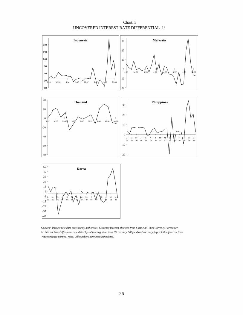
Chart 5 shows the results using expected depreciation calculated from the

Financial Times Currency Forecaster. Similar to the real interest rate results,

negative interest rate differentials are found for Malaysia, Philippines, Korea and

Indonesia at the beginning of 1998 and for Thailand in July 1997. Also, very high

interest differentials (larger than 20 percent per annum) emerge from March 1998

in all the countries. The results from the uncovered interest rate differentials

confirm that there is little evidence of overly tight monetary policies in Asia at the

beginning of the crisis through early 1998.

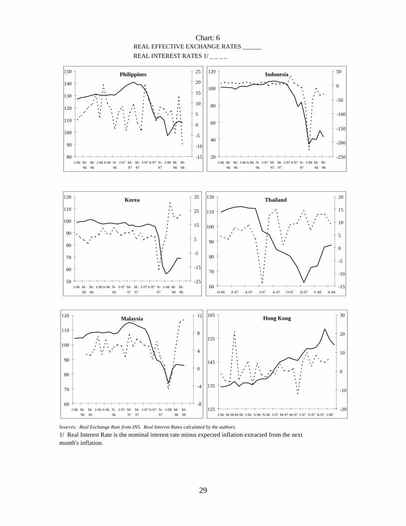
The relationship between real interest rates and real exchange rates for the

five countries considered is shown in Chart 6. As explained in the theory section,

the traditional approach stresses that one should expect a positive correlation

between exogenous interest rate shocks and the exchange rate. We have no

independent data on monetary policy shocks but it is still interesting to look at the

simple correlations. The evidence is mixed, in the period of the crisis July/1997 to

July/1998, a fairly positive correlation exists for Hong Kong (0.55), Indonesia

(0.57), Malaysia (0.42), and Philippines (0.13). In contrast, we observe a negative

correlation in Korea (-0.46) and Thailand (-0.46).

Chart 7 shows the relationship between real interest and exchange rates in

the other crisis episodes. A positive correlation is evident in all the cases. In

Mexico (1994), the recovery of the real exchange rate happened when real interest

11The residual in the uncovered interest differential is sometimes identified automatically as the risk premium.

28

rates were raised in the second quarter of 1995. Likewise, in Mexico (1982) the

real exchange rate recovered when interest rates were raised in mid-1982. In Chile

(1982), interest rates were raised shortly after the crisis but allowed to fall

immediately thereafter. The RER recovered initially but the recovery was not

sustained. A notable feature is that the increases in real rates in these cases were

much sharper than those seen in most of the Asian crisis countries.

One could analyze econometrically the relationship between real exchange

rates and real interest rates by looking at historical data to increase the number of

data points available.

29

REAL EFFECTIVE EXCHANGE RATES ______

REAL INTEREST RATES 1/ _ _ _ _

Sources: Real Exchange Rate from INS. Real Interest Rates calculated by the authors.

1/ Real Interest Rate is the nominal interest rate minus expected inflation extracted from the next month's inflation.

Chart: 6

Indonesia

20

40

60

80

100

120

J-96 M-96

M-96

J-96 S-96 N-96

J-97 M-97

M-97

J-97 S-97 N-97

J-98 M-98

M-98

-250

-200

-150

-100

-50

0

50

Korea

50

60

70

80

90

100

110

120

J-96 M-96

M-96

J-96 S-96 N-96

J-97 M-97

M-97

J-97 S-97 N-97

J-98 M-98

M-98

-25

-15

-5

5

15

25

35 Thailand

60

70

80

90

100

110

120

D-96 F-97 A-97 J-97 A-97 O-97 D-97 F-98 A-98-15

-10

-5

0

5

10

15

20

Malaysia

60

70

80

90

100

110

120

J-96 M-96

M-96

J-96 S-96 N-96

J-97 M-97

M-97

J-97 S-97 N-97

J-98 M-98

M-98

-8

-4

0

4

8

12

Philippines

80

90

100

110

120

130

140

150

J-96 M-96

M-96

J-96 S-96 N-96

J-97 M-97

M-97

J-97 S-97 N-97

J-98 M-98

M-98

-15

-10

-5

0

5

10

15

20

25

Hong Kong

125

135

145

155

165

J-96 M-96 M-96 J-96 S-96 N-96 J-97 M-97 M-97 J-97 S-97 N-97 J-98-20

-10

0

10

20

30

30

REAL EFFECTIVE EXCHANGE RATES ______ REAL INTEREST RATES 1/ _ _ _ _

Sources: Real Exchange Rate from INS. Real Interest Rates calculated by the authors.

1/ Real Interest Rate is the nominal interest rate minus expected inflation extracted from the next month's inflation.

Chart: 7 (Latin America)

Brazil

0

20

40

60

80

100

120

140

1994JAN

1994JUL

1995JAN

1995JUL

1996JAN

1996JUL

1997JAN

1997JUL

1998JAN

0

10

20

30

40

50 Argentina

140

150

160

170

180

1995JAN

1995JUL

1996JAN

1996JUL

1997JAN

1997JUL

1998JAN

0

5

10

15

20

25

Mexico I

0

40

80

120

160

200

1981JAN

1981JUL

1982JAN

1982JUL

1983JAN

1983JUL

1984JAN

1984JUL

-120

-100

-80

-60

-40

-20

0

20Mexico II

0

20

40

60

80

100

120

140

1993 JAN1993 JUL1994 JAN1994 JUL1995 JAN1995 JUL

-25

-15

-5

5

15

25

Chile

0

50

100

150

200

250

300

1980JAN

1980JUL

1981JAN

1981JUL

1982JAN

1982JUL

1983JAN

1983JUL

1984JAN

1984JUL

-60

-40

-20

0

20

40

60

31

Impulse Response of Exchange Rate Changes due to Innovations in Interest Rate Changes (Country Code: THAI-Thailand, KOR-Korea, MLS-Malaysia, PHIL:Philippines, IND: Indonesia )

Note: VAR estimation, using daily data from 06:01:1997 to 05:18:1998.

Contains a constant term and 12 lags of each variable.

Dependent Variable (DER followed by country code): first log difference

of exchange rate vis-à-vis US$

Independent Variable (DIN followed by country code): first difference

of daily call rate

Source: Data obtained from authorities and IMF staff estimates.

Chart 8

-0.010

-0.005

0.000

0.005

0.010

0.015

0.020

1 2 3 4 5 6 7 8 9 10

Response of DERTHAI to DINTHAI

Response to One S.D. Innovations ± 2 S.E.

-0.015

-0.010

-0.005

0.000

0.005

0.010

0.015

1 2 3 4 5 6 7 8 9 10

Response of DERKOR to DINKOR

Response to One S.D. Innovations ± 2 S.E.

-0.010

-0.005

0.000

0.005

0.010

0.015

1 2 3 4 5 6 7 8 9 10

Response of DERPHIL to DINPHIL

Response to One S.D. Innovations ± 2 S.E.

-0.010

-0.005

0.000

0.005

0.010

0.015

1 2 3 4 5 6 7 8 9 10

Response of DERMLS to DINMLS

Response to One S.D. Innovations ± 2 S.E.

-0.02

-0.01

0.00

0.01

0.02

0.03

0.04

1 2 3 4 5 6 7 8 9 10

Response of DERIND to DININD

Response to One S.D. Innovations ± 2 S.E.

32

Sample:June, 1997Sep, 1997

July, 1997Oct, 1997

Aug, 1997Nov, 1997

Sep, 1997Dec, 1997

Oct, 1997Jan, 1998

Nov, 1997Feb, 1998

Dec, 1997Mar, 1998

Jan, 1998Apr, 1998

WholeSample

Fixed Effects Panel(with 1 lag of independent variable)coeff. Est -0,0003 -0,0002 -0,0001 -0,00006 -0,00002 -0,0001 -0,002 -0,002 -0,00009t-stat -2.49** -1.66* -1,21 -0,29 -0,11 -0,38 -1.61* -1.76* -0,52

Country by Country regression(with 1 lag of independent variable)Indonesiacoeff. Est -0,0006 -0,0005 -0,0006 -0,0003 0,0008 0,0005 0,0003 0,0004 -0,0004t-stat -2.95** -2.27** -2.04** -0,258 0,31 0,14 0,63 0,66 -0,71Malaysiacoeff. Est 0,0001 0,00008 0,002 0,005 0,001 0,002 0,001 -0,002 0,0001t-stat 0,28 0,16 1.00 2.21** 0,4 0,37 0.20 -0,33 0,19Philippinescoeff. Est -0,0002 0,00003 0,000006 -0,000004 -0,000007 -0,0003 -0,0007 -0,006 -0,00004t-stat -0,41 0,14 0,02 -0,01 -0,02 -0,65 -3.51** -3.63** -0,19Koreacoeff. Est 0,0002 -0,002 -0,01 -0,003 0,002 -0,001 0,002 0,003 -0,0009t-stat 0,39 -2.32** -3.16** -0,78 -0,45 -0,32 0,55 0,83 -0,38Thailandcoeff. Est 0,001 0,001 0,0006 0,001 0,001 -0,001 0,0009 -0,0008 0,0008t-stat 1,11 1,33 0,54 0,67 0,55 -0,56 0,33 -0,36 0,82Note: Results of regressions using daily data. Significance at 10% and 5% level are denoted by * and **.

Individual and Panel Data Regression of Nominal Exchange Rates on Nominal Interest RatesTable 5

33

However, in this paper, we are restricting our attention to the correlation

between these variables in crisis episodes. There are two alternative approaches.

One is to extend the sample of crisis episodes and run a panel data set regression.

This approach is followed in Goldfajn and Gupta (1998). Another approach is to

use higher frequency data, i.e., daily data. In this case, we will need to focus our

attention on the relationship between nominal exchange rates (national currency per

unit of dollar) and nominal interest rates. Chart 8 shows the impulse responses of

a vector autoregression of the changes in nominal interest rates on the changes in

nominal exchange rates. The results show that the effect of a shock in interest rates

on the exchange rate is insignificant in all the five cases (perhaps, the only exception

is Philippines). This confirms previous results obtained in Ghosh and Phillips (1998)

and Kaminsky and Schmukler (1998).

It is interesting to observe how the correlation of interest rates and exchange

rates has evolved over time. Table 5 shows rolling regressions for the five Asian

crisis cases plus a panel regression. As expected, when running the panel regression

for the whole sample one does not obtain a negative correlation. However, there

are periods where there was a negative correlation between the variables. In

particular, one obtains a significant negative correlation in the period from the

Thailand crisis to October 1997 and from January to April 1998. Looking at

particular countries, the strongest negative correlation occurs in Indonesia and

Korea in 1997 and Philippines in 1998. The only positive correlation is found for

Malaysia in the last four months of 1997.

In summary, this section has two main results. First, we find little evidence

that monetary policy was overly tight in the immediate aftermath of the crises.

34

Second, there is no clear evidence that higher interest rates led to weaker exchange

rates. If anything, we find that there are periods where higher rates led to stronger

exchange rates.

IV. OPTIMALITY AND TRADEOFFS IN RAISING INTEREST RATES

The previous section considered the question whether interest rates were

very high during the Asian crises. While we don’t find evidence of excessively tight

monetary policy at the beginning of the crisis, our analysis so far has precluded any

discussion on whether, in the context of the Asian crises, there was a case to be

made in favor of high interest rates. Even if one accepts the hypothesis that

temporary rise in interest rates can stabilize exchange rates, the costs of using

monetary policy may be too large to justify high rates. This section evaluates the

benefits of raising interest rates to defend the currency with the alternative of letting

the exchange rate overshoot.

The alternative to raising interest rates is not necessarily a free fall in the

exchange rate, although the risk of a spiral inflation-depreciation exists. It is

possible that large declines in the exchange rate could prompt the operation of

automatic stabilizers. In the medium term, the real depreciation of the currency

could induce a reversal of the current account and would generate capital inflows

that would appreciate the currency. In the short run, the expectations of future

recovery could bring stabilizing speculators back to the market.

The question of raising interest rate to cause nominal appreciation, or at

least stabilize the currency, is traditionally reconciled with the output-inflation

trade-off. Sustaining tight monetary policy can have negative effects on output,

unemployment, and investment, the latter with important repercussions in the long

35

run. On the other hand, allowing the exchange rate to overshoot has a negative

effect on inflation. In addition, too large an exchange rate misalignment for too long

may also cause recession and layoffs in the non-tradable sector.

The proponents of using higher interest rates to stabilize the currency argue

that the increase in interest rates need only be temporary and, therefore, the effect

on output is limited. Few will dispute that a prolonged period of very high interest

rates may produce such a decline in output that may tilt the trade off in favor of

letting the exchange rate overshoot. In fact, it is well known from the experiences

during the great depression and subsequent stock market crashes, that the optimal

response of a first round of corporate failures is to increase liquidity (or,

equivalently, reduce interest rates) rather than sustain a tight monetary policy.

It is important to consider the issue of raising rates along with factors that

are not part of the conventional trade-off.12 The relative effect of interest and

exchange rates on the balance sheets of corporations (in the banking system, in

particular) warrants equal attention. In this framework, the key is to evaluate the

relative exposure of companies to changes in interest rates and exchange rates. The

increases in interest rates raise the cost of borrowing to highly leveraged companies

and, in the banking system, increases in interest rates may significantly reduce

profits due to the existence of maturity mismatches. In addition, failures in the non-

bank corporate sector may induce failures in the banking system through increases

in non-performing loans. On the other hand, in the same manner that increases in

interest rates may induce problems in the corporate sector, an over depreciated

currency increases the funding costs of corporations exposed to foreign currency.

12See Furman and Stiglitz (1998) for a broad-based analysis of this issue.

36

In particular, in developing countries with fixed exchange regimes, banks and

companies tend to have a currency mismatch in their portfolio and are vulnerable

to large changes in the exchange rate. One of the reasons foreign investor become

skeptical about the outlook of an economy undergoing rapid currency devaluation

stems from the fact that the domestic corporate sector becomes extremely fragile

as the devaluation increases the foreign debt burden in domestic currency

denomination. An economy’s exposure to foreign debt is a crucial consideration in

the policy trade-off.

The evidence on the relative cost of interest rate versus exchange rate

changes on the corporate sector is scarce. For the banking system, the study by

Demirguc-Kunt and Detragiache (1997) for 30 developing and industrial countries

show that high interest rates substantially increase the probability of a financial

crisis while depreciations of currencies have little, if any effect. Goldfajn and Gupta

(1998) find that for countries that are experiencing simultaneous banking and

currency crises, countries with tight monetary policy have a significantly lower

probability of success.13

So how can policy makers distinguish between countries that will suffer more

from interest rates and the ones that will be more vulnerable to currency

depreciation? In Table 6, we show, for the Asian crisis cases, a few indicators that

hint at the relative cost of interest rate versus exchange rate changes. Table 7 shows

the same indicators for other cases of currency crises. Corporate debt/equity and

credit of private sector/GDP ratios indicate how extended the private sector is, as

13In the context of the Asian crises, evidence suggests that Korea and Thailand had severe banking problems prior

to the currency collapse.

37

well as its vulnerability to interest rate hikes. External debt, short term debt in

particular, indicate the extent of foreign currency exposure. From the perspective

of the traditional trade-off (output versus inflation), the overall low rates of

inflation and large declines in output in the five Asian crisis cases suggest that the

relative cost of an additional increase in interest rates may have been higher than an

additional decline in the exchange rates. This is particularly true if a comparison

with the previous Latin American currency crises is made, where inflation rates

tended to be higher and output declines smaller. The only caveat is if the lags in

Asia were to imply a larger passthrough in the future, as suggested in section II.B,

and, therefore, a higher inflation.

A different perspective emerges if one considers the relative exposures to

exchange rates versus interest rates. Indonesia had the highest external debts and

the largest real depreciation compared to Asia and, also, to other currency crises

cases. This suggests a large exposure to exchange rate change, and the importance

of stabilizing the currency. Korea, with relatively a low external debt (compared

to both Asian and other crises) and high debt/equity ratio of domestic corporates

suggests a high exposure to interest rate increases. In the case of Thailand, both the

high debt to equity ratio and the large ratio of credit to the private sector as a

percentage of GDP suggests a large exposure to high interest rates as well. This

assessment, in conjunction with the traditional trade-off (large drop in output and

relatively low inflation), suggests that a trend towards lower rates was beneficial

for Korea and Thailand.14 Philippines had a relatively high real rate if one considers

14The case of Thailand is not very clear-cut. The fact that the country had nearly 20% of its external debt in short

term borrowing indicates that there was substantial currency exposure as well.

38

that its debt to equity and private credit to GDP ratios are relatively low and the

expected decline in output is moderate. In contrast, Malaysia had a relatively low

rate considering the low debt to equity ratio (although the credit to the private

sector was substantial). The choice of policy stance during a financial crisis is

crucial, given the high stakes involved. Overly tight monetary policy might

exacerbate the crisis, while an overly depreciated currency can cause serious

problems as well. The above discussion highlights the importance of reconciling the

traditional trade-off with corporate balance sheet considerations. In light of the

evidence, an across the board tightening of monetary policy for the Asia 5 was

difficult to defend. Thailand and Korea were, according to the selected indicators,

more susceptible to high rates than currency devaluation, thus requiring an easing

of the monetary policy. It is difficult to make the same case for Indonesia and

Philippines though. Finally, Malaysia was the clearest candidate for a relatively soft

stance.

39

Thailand Malaysia Philippines Indonesia Korea

Traditional Trade-off (growth versus inflation):CPI Inflation Forecast 1/ 7,6 7,2 5,3 42,0 8,5Growth Projection for 1998 -8,0 -4,0 -0,7 -12,0 -5,0Effective Real Exchange Rate on April, 1998 (June, 97 =100) 66,3 77,2 78,5 47,7 72,6

Balance Sheet Trade-off:Corporate Debt/Equity Ratio (in percent) 419 200 63 950 518Credit ot Private Sector/GDP Ratio, end-1997 (in percent) 145 162 56 61 74External Debt (as a percent of GDP) 59,6 43,6 62,1 78,0 51,2 of which: short term debt 19,4 10,4 15,7 15,0 14,3

Monetary Policy:Nominal Interest Rates on July 1998 16,1 11,0 14,9 79,2 13,0Real Interest Rates 2/ 7,9 3,5 9,1 26,2 7

1/ Expected Inflation for the second half of the year annualized. Staff Estimates.

2/ Real interest rate calculated using the exact formula (1+i)/(1+inf) - 1.

Country Notes:Malaysia: Nominal interest rate is three month interbank rate. External Debt numbers are end-1997.Philippines: Nominal interest rate is the three month Treasury Bill. Effective Debt/equity ratio is based on a sample of companies (full data n.a.) and based on net rather than gross debt. Impact on corporate sector based on 1997 data.Korea: Nominal interest rate is the three month CD rate. External Debt numbers are end-1997. Debt/Equity ratio is based on top 30 Chaebols. Indonesia: Nominal rate is the one month interbank rate. External debt numbers include $ domestic debt and GDP is calculated as 4 times June quarter GDP at average e/r for June quarter. Debt equity ratio calculated using market value of equity of incorporated co's only (equity is thus understated and D/E overstated). Simple monthly interest rates are converted to represent compounded annualized rates. Thailand: Nominal interest rate is the one month repurchase rate. External Debt numbers are end-1997.

Table 6: Asia 5 -- Selected Indicators for Policy Trade-off, 1998

40

Chile ('82) Mexico ('82) Mexico ('94) Sweden ('92) UK ('92)

Traditional Trade-off (growth versus inflation):CPI Inflation 1/ 30,1 208,7 52,0 4,4 1,02Growth Rate 2/ -2,3 -4,1 -7,5 -1,2 1,0Effective Real Exchange Rate, (crisis period = 100) 76,7 55,5 75,4 76,3 98,1

Balance Sheet Trade-off:Credit to Private Sector/GDP, in the year of devaluation (%) 68,2 7 40 54 127External Debt (as a percent of GDP) 67,3 52,1 37,3 #na #na of which: short term debt 12,3 15,2 7,0 #na #na

Monetary Policy:Nominal Interest Rates on the Month of the Crisis 34,8 34,2 26,4 82,38 8,8Real Interest Rates 3/ 8,1 -24,6 7,3 78,5 5,56

1/ 12 month inflation from the onset of the crisis. The same holds for REER.

2/ Annual GDP growth rate from the quarter of the crisis.

3/ Real interest rate calculated as the nominal interest minus CPI inflation, both defined above.

Country Notes:Chile: Nominal interest rate is the deposit rate.Mexico: Nominal interest rate is treasury bill rate. Sweden: Nominal rate is the overnight call money rate. UK: Nominal interest rate is the overnight interbank rate.

Table 7: Selected Indicators for Policy Trade-off, Other Currency Cases

41

V. CONCLUSION

This paper evaluated monetary policy and its relationship with exchange rate

in the five Asian crisis countries. The findings are compared to previous currency

crises in recent history. The paper argues that there was room to believe that the

exchange rates had overshot during the crisis and that further declines were not

desirable, naturally raising the question of the appropriate policies to revert this

overshooting.

The paper finds that there is no evidence of overly tight monetary policy in

the Asian crisis countries in 1997 and early 1998. Negative real rates were

encountered for Indonesia, Korea and Malaysia in early 1998 and for Thailand in

the third quarter of 1997. In addition, real interest rates in Indonesia, Malaysia and

Philippines are below their pre-crisis levels. There is no evidence of large

uncovered interest rate differentials in the Asian crisis countries in 1997 and early

1998.

There is also no evidence that high interest rates led to weaker exchange

rates. Simple correlations using monthly data provide mix results and vector

autoregression model estimations with daily data imply, if anything, that higher

interest rates are associated with stronger exchange rates. There are a couple of

issues one should consider regarding this result. First, the Asian crisis generated

an increase in the risk premium demanded for holding the crisis countries assets.

This increase is associated with both a higher interest rate and a more depreciated

exchange rate that would tend to bias the result in favor of finding a perverse effect

of interest rates on the exchange rate. However, the perverse effect is not found

despite this natural bias. Second, the paper recognizes that the relationship between

42

interest rate and exchange rates is more complex and is affected by other

macroeconomic policies and the political support and credibility they enjoy. In

absence this credibility, even large increases in interest rates would not be

successful in stemming exchange rate depreciations. Third, in order to test more

rigorously this result, one needs to assemble a larger data set, which is only

available once a great number of currency crises are considered. This larger

exercise is performed in a separate paper (Goldfajn and Gupta, 1998).

The paper highlights the need to reconcile the traditional interest rate-

exchange rate trade-off with a corporate balance sheet approach. The cost

associated with high interest rates to stabilize the currency can be overwhelming if

the banking sector is fragile. On the other hand, if the corporate sector is heavily

exposed to foreign debt, then increasing interest rates may be the appropriate

policy. Monetary policy in the aftermath of currency crisis requires close attention

to these issues.

43

REFERENCES

Baig, Taimur, and Ilan Goldfajn, 1998, “Financial Market Contagion in the Asian Crisis,”IMF Working Paper WP/98/155, International Monetary Fund.

Chinn, Menzie, 1997, “Before the Fall: Were East Asian Currencies Overvalued?”NBER Working Paper No. 6491 (Cambridge, Massachusetts: MIT Press).

Demirguc-Kunt and Detragiache, 1997, “The Determinants of Banking Crises: Evidencefrom Industrial and Developing Countries.” IMF Working Paper WP/97/106.International Monetary Fund.

Drazen, Alan, and Paul, Masson 1994, “Credibility of Policies versus Credibility of Policymakers,” Quarterly Journal of Economics, 109(3), August, 735-54.

Dornbusch, Rudiger, 1976, “Expectations and Exchange Rate Dynamics,” Journal ofPolitical Economy, 84(6), December, 1161-76.

Dornbusch, Rudiger, 1998, “East Asian Themes,” At internet website http://web.mit.edu.

Eichengreen, Barry, Andrew Rose and Charles Wyplosz, 1994, “Speculative Attacks onPegged Exchange Rates: An Empirical Exploration with Special Reference to theEuropean Monetary System,” NBER Working Paper 4898.

Flood, Robert, and P. Garber, 1984, “Collapsing Exchange Rate Regimes: Some LinearExamples,” Journal of International Economics, vol. 17, Aug.

Furman, Jason and Joseph Stiglitz, 1998, “Economic Crises: Evidence and Insights fromEast Asia,” prepared for Brookings Panel on Economic Activitiy, Washington,D.C., September 3-4.

Ghosh, Atish, and Steven Phillips, 1998, “Interest Rates, Stock Markets Prices andExchange Rates in East Asia” (unpublished, International Monetary Fund,Washington, DC).

Goldfajn, Ilan, and Rodrigo Valdés, 1996, “The Aftermath of Appreciations,” NBERWorking Paper no. 5650 (Cambridge, Massachusetts: MIT Press). Also,Quarterly Journal of Economics. Vol. 114, # 1. 229-262.

Goldfajn, Ilan, and Poonam Gupta, 1998, “Does monetary policy stabilize the exchangerate?” (unpublished, International Monetary Fund, Washington, DC).

Goldstein, Morris, 1998, The Asian Financial Crisis: Causes, Cures, and SystemicImplications. (Washington: Institute for International Economics).

44

Goldman Sachs, 1997, “New Tools for Forecasting Exchange Rates in EmergingMarkets: Goldman Sachs Dynamic Equilibrium Emerging Markets ExchangeRates (GSDEEMER),” Economic Research, New York

Goldman Sachs, 1998, “Emerging Market Currency Analyst,” Economic Research, NewYork.

Kaminsky, Graciela and S. Schmukler, 1998, “The Relationship Between Interest Ratesand Exchange Rates in Six Asian Countries,” (unpublished, The World Bank,Washington).

Kindelberger, Charles P. , 1978, Manias, Panics and Crashes: A History of FinancialCrises. (New York: Basic Books, Inc., Publishers).

Kochhar, Kalpana, Prakash Loungani and Mark Stone, 1998, “The Asian Crisis:Macroeconomic Developments and Policy Lessons,” Forthcoming in IMFWorking Paper Series, International Monetary Fund.

Krugman, Paul, 1979, “A Model of Balance of Payment Crises,” Journal of Money,Credit and Banking, vol.11 (3), 311-325.

Krugman, Paul, 1998a, “What Happened to Asia?” At internet websitehttp://web.mit.edu.

Krugman, Paul, 1998b, “Will Asia Bounce Back?” At internet websitehttp://web.mit.edu.

Radelet, Steven, and Jeffrey Sachs, 1998, “The East Asian Financial Crisis: Diagnosis,Remedies, Prospects,” Paper prepared for the Brookings Panel (Washington:Brookings Institute).

Obstfeld, Maurice, 1994, “The Logic of Currency Crises,” Cahiers Economiques etMonetaires (Banque de France, Paris), 43, 189 -213.

Roubini, Nouriel, Paolo Pesenti and, Giancarlo Corsetti, 1998, “What Caused the AsianCurrency and Financial Crises,” at Internet Websitewww.stern.nyu.edu/~nroubini/asia/Asiahomepage.html.

Stiglitz, Joseph, 1998, “Knowledge for Development: Economic Science, EconomicPolicy and Economic Advice”, Annual Bank Conference on DevelopmentEconomics (Washington: The World Bank).

45

Appendix

Description of Monetary Policy in the Asian Crisis Cases

Korea

Korean authorities reacted to counter the steep decline in the value of the

won during the winter of 1997-98 by raising overnight inter-bank interest rates. By

January 1998, the overnight rate had been raised to around 30 percent (see Chart

3A), subsequently leading to sizable increases in short and long term corporate

borrowing rates as well.15 The maintenance of the high rates managed to halt the

persistent decline of the currency. The high interest rates also slowed monetary

growth. By the end of March 1998, reserve money had contracted below the

indicative Fund program target,16 thus necessitating a slight downward revision of

the end-June indicative target.

Foreign exchange market stability was restored in February, 1997. The call

rate was gradually decreased as a response to the improvement of the won’s value.

By early May, the overnight call rate had come down to 18 percent,17 while at the

same time the currency had recovered 25 percent since its end-1997 levels. The

lowering of the interest rate brought some relief to the highly leveraged institutions.

The monetary authorities kept close vigil on the currency markets though, and

resolved to tighten monetary policy by virtue of higher rates in case of any hint of

renewed exchange rate instability.

15By February 1998, cost of new borrowing had increased to 26 percent for commercial paper and overdrafts,

21 percent for corporate bonds, and 18 percent for bank loans.16The March 1998 reserve money figure was 22 trillion won, as opposed to the program target of 23.6 trillion

won.17The easing in borrowing rate was also reflected in the early May three-year corporate bond rate, which fell to

18 percent.

46

Malaysia

In the aftermath of the contagion spread by the baht devaluation, the

Malaysian ringgit faced speculative attacks. During the speculative attack episode

in mid-July 1997, overnight call rates rose up to 35 percent (see Chart 3B). But

since the attempts to hold up the currency were not successful, the authorities

decided to rely less on interest rate instruments to tackle exchange rate volatility.

Interest rates were lowered almost to pre-crisis levels, and more emphasis was

given to various measures to reduce expenditure and credit growth in the

economy.18 Despite these measures, the rhetoric against speculators and measures

to restrict trading in the domestic stock and currency market led to sustained

decline of the ringgit.19

The rationale provided by the Malaysian authorities about their unwillingness

to pursue a vigorous interest rate defense was twofold. First, there was consensus

among political leaders that the adverse impact of high interest rates in impeding

growth made it a very delicate policy choice. Furthermore, the strong contagion

effects from the rest of the region appeared likely to overwhelm any stability

induced by higher rates. Nevertheless, the authorities, in the wake of their

discussion with Fund, Bank, and ADB officials, recognized the need to supplement

the existing policies to curb monetary growth with a flexible short term interest rate

policy that will allow them to respond to renewed pressure in the currency market.

The authorities acknowledged the need to do this in light of the likelihood that the

cost of prolonged period of undervaluation was higher than that of short term

18Such as restricting property sector lending and loans for financing stock market activity.

19The ringgit fell, from 2.57 to the dollar in July 1997, to 4.39 in January 1998,.

47

interest rate hike.20 They asserted to maintain a forward looking interest rate policy

that would ensure real interest rates of 3-4 percent on 3-month deposit instruments.

Philippines

The de facto peg maintained by authorities of the Philippines since late 1995

became unsustainable in July 1997 in the face of regional currency crises, leading

to a free floating peso. During the period when the peso-US$ exchange rate was

kept virtually constant, the central bank had in effect eliminated the scope for

independent monetary policy, but continued to follow previously established base

money targets. The floating of the peso eliminated this inconsistency in the policy

framework.

The base money targeting was carried out by adjusting the overnight and

term repos, as well as the reverse repos. However, holding the interest rate low

was a long standing priority, and after a short period of tight monetary policy in

mid-1997,21 monetary policy became largely accommodative between September

1997 and January 1998. The relatively lower rates (as opposed to market rates)

offered by the central bank brought the amount of open market operations almost

to zero by January 1998. The period was also accompanied by a large shortfall of

net international reserves (NIR) from the program target. Policy makers seemed to

acknowledge the need to stabilize the exchange rate and maintain target NIR levels

but they strongly disputed the effectiveness of raising interest rates noting that

higher rates would adversely affect ailing banks and enterprises, thus causing more

20The increase in import costs for the corporate and industrial sector, as well as devaluation induced inflationary

pressures.

21This was done mostly through raising policy interest rate above market rates, and by increasing liquidity reserverequirements, which are the obligatory treasury bill holdings of the banks.

48

panic among the agents and would be unlikely to stem the pressure from the

regional contagion. They found the existing gap22 between bank lending rates and

other rates as excessive, and wanted to pursue measures to reduce them. However,

it is possible that the high rates reflected, to a large extent, the difficulty faced by

the banks to build badly needed capital and provision for non-performing loans.

Indonesia

After facing sustained selling pressure in the wake of the baht devaluation,

the Indonesian authorities relinquished the rupiah peg in August 14, 1997. This

event was preceded by futile interest rate defense in late July and early August.23

The weeks subsequent to the free floating of the rupiah saw the currency slide to

nearly 4000 to the dollar, from the pre-crisis level of approximately 2500. In

response, the authorities announced a wide range of reform initiatives, and sought

IMF assistance in stabilizing the economy. During October and early November the

currency showed some signs of stability. At the same time, interest rates came

down to almost pre-crisis levels.24

However, this respite was short-lived. By late November, due to major

uncertainty regarding the actual implementation of the economic reforms, increasing

pessimism of the extent of economic contraction, as well as lack of confidence in

the political leadership, the rupiah tumble drastically. A vicious circle of

devaluation ensued, and by late January, the rupiah crossed over the 13,000 to the

dollar level. The authorities tried to stem the currency slide by pursuing monetary

22In January 1998, the end of period prime lending rate was 25.4 percent and the 1-month PHIBOR was 23.6

percent, as opposed to BSP 1-month rate of 16.9 percent.

23At one point the overnight JIBOR was pushed over 42 percent.

24In October, the 30 day JIBOR was 20.6 percent, barely 3 percent over July levels.

49

tightening. Overnight JIBOR was raised to nearly 40 percent by end-January, while

the weighted average rate in the inter-bank market rose to over 90 percent (see

Chart 3B).

But the high interest rates failed to bring prolonged respite to the market.

A combination of sharp decline in the value of the rupiah and steep increase in

domestic interest rates hurt the balance sheet of most firms tremendously.25 Thus

despite the resolve to support the currency and contain inflationary pressures, the

authorities found their objective floundering in the face of an across the board

liquidity crisis. The immediate impact of this crisis was reflected in the

segmentation of the banking market, where the weaker banks relied on extensive

liquidity support, and the better off banks had to deal with interest rates that were

persistently above 30 percent. Between November 1997 and March 1998, liquidity

support for banks increased by the equivalent of about 8 percent of GDP. The

inflationary spiral and the lack of confidence in the banking sector led to increased

demand for currency despite the high interest rates. As inflation rates picked up,

real interest rates actually became substantially negative in early 1998. The low real

rates limited the ability of the authorities to absorb excess liquidity through open

market operations.

Thailand

25It was estimated by Fund staff that majority of the publicly listed non-bank companies were technically bankrupt

by end-January. Another estimate of the Bank of Indonesia indicated that banks representing over 70 percentof private banking sector assets had capital (risk adjusted) below the regulatory requirements.

50

Thailand’s monetary policy typifies the challenges of an interest rate defense

during a currency crisis. After heading off speculative attacks at the beginning of

1997,26 the Thai authorities faced renewed attacks during the months of May and

June. Despite vigorous defense by means of forward market intervention,

imposition of various restrictions to make the short sale of baht costly, and sharp

interest rate hike,27 the selling pressure on the baht proved to be overwhelming.

The resulting and potential loss of reserves forced the authorities to release the baht

from its peg on July 2.

The authorities followed the free floating of the baht with a relatively

accommodating monetary policy, as reflected by the fall of inter-bank interest rates

to nearly pre-crisis levels by mid-August, when overnight rates fell to 14.35

percent. This was done with the expectation of the market renewing its confidence

in the ongoing reform efforts, and also to help ease the cost of debt servicing for

the ailing banks and finance companies. The expectation, however, proved to be

wrong as political uncertainties and delays in pushing through reforms etc. kept

market confidence low. The exchange rate continued to face pressure, and the

authorities had to allow rates to rise again. Overnight repo rates jumped to 23

percent in September (see Chart 3B), while minimum lending rates rose by about

200 basis points in desperate attempts to halt the slide of the baht. Interest rates

did not rise uniformly though. The Thai market began to segment at this stage as

the large domestic banks sought to place excess reserves in risk free assets, thus

26Market commentators suggest that the baht was attacked by speculators in late January/ early February. The

central bank defended this attack successfully, and subsequent to the defense interest rate declined noticeably,e.g. overnight inter-bank rates came down to 8.55 percent in March, as opposed to 12.8 percent in February;over the same time period, overnight repo rates declined to 8.7 percent from 12.24 percent.

27By late June, overnight rates reached 19 percent.

51

commanding a lower overnight borrowing rate28, whereas smaller institutions,

increasingly short of the required collateral, continued to face relatively high

interest rates of over 20 percent in the inter-bank market. Any possibility of the

interest rates being lowered was subsequently dashed as widespread regional

contagion from November onwards brought further selling pressure on the baht.

This led to across the board interest rates staying above 19 percent through the

spring of 1998.

One aspect of the interest rate movement during the ongoing crisis has been

the relative rigidity of the broader rates’ structure. Despite the big fluctuations in

the overnight inter-bank rates, deposit and lending rates remained relatively stable

during the episode. The Thai authorities imposed a deposit rate cap in September

1997,29 done primarily to limit moral hazard on the part of financial institutions

covered by the bailout guarantee. Additionally, the large banks had little incentive

to offer higher rates to depositors who were already shifting their deposits from

smaller, weaker banks to them.30 On the lending side, banks were reluctant to

charge higher rates which will lead, under the prevailing uncertain economic

environment, to an increase of the average riskiness of loans. Thus, despite a tight

monetary policy, the broader rates have been generally lower.

28In mid-October, over night repo rates fell to 12 percent, largely driven by rates as low as 8 percent for the most

creditworthy banks.

29The interest rate cap constrained deposit rates to 300 basis points above the average deposit rate of the fourmajor banks.

30Some smaller, ailing banks have tried to raise rates and offered benefits to attract depositors.