Embed Size (px)
Citation preview
Departamento de Sistemas Informáticos y Comutación
Universitat Politècnica de València
DESIGN AND IMPLEMENTATION OF AN
ATRIAL FIBRILLATION DETECTOR BASED
ON NEURAL NETWORKS
Master Thesis
Master’s Degree in Artificial Intelligence, Pattern
Recognition and Digital Imaging
Author: Xavier Ibáñez Català
Tutor: Roberto Paredes Palacios
2014-2015

Design and Implementation of an Atrial Fibrillation Detector Based on Neural Networks
2
Master’s Degree in Artificial Intelligence, Pattern Recognition and Digital Imaging
Master Thesis Xavier Ibáñez Català
3
Resumen La fibrilación auricular (FA) es la arritmia sostenida más frecuente en la población,
aumentando su prevalencia con la edad de los pacientes. La sintomatología de la FA reduce
considerablemente la calidad de vida. No obstante, la mayor causa de morbimortalidad asociada
a la FA es consecuencia del riesgo aumentado de sufrir un accidente cerebrovascular por un
trombo de génesis cardiaca. Es por ello que existe un gran interés clínico en el diagnóstico
precoz, tratamiento y control de los pacientes con FA.
Este Trabajo Fin de Máster tiene como objetivo el diseño y desarrollo de un detector de FA
que sólo utilice la información contenida en los intervalos RR de un segmento de 30 segundos
de electrocardiograma. Para ello se emplean redes neuronales y se exploran diferentes técnicas
para mejorar sus capacidades de aprendizaje. El detector desarrollado se integra en una
aplicación comercial de procesado de señal electrocardiográfica de larga duración. Tras la
integración, el detector es posteriormente testado según los estándares de aplicación en este
ámbito, demostrándose su eficacia.
Palabras clave: ECG, electrocardiografía ambulatoria; fibrilación auricular, detección
basada en RR, redes neuronales.
Abstract Atrial fibrillation (AF) is the most common sustained arrhythmia, increasing its prevalence
with the age of the patients. The symptoms of AF considerably reduce the quality of life.
However, the most important cause of morbid-mortality associated to AF is consequence of an
augmented risk of suffering a stroke as a result of a cardiogenic thrombus. Because of this,
clinical community is very interested in an early diagnosis, treatment and control of the patients
with AF.
The objective of this Master Thesis is to design and develop an AF detector which only uses
the information contained in the inter-beat interval sequence of an electrocardiogram segment of
30 seconds. To achieve this goal, artificial neural networks are employed and several
approaches to improve their learning capabilities are explored. The developed detector is
integrated in a commercial software solution to analyze long-term electrocardiograms. After the
integration, the detector is tested according to the standards applying to this sector,
demonstrating its effectiveness.
Keywords: ECG, ambulatory electrocardiography, atrial fibrillation, RR-based detection,
neural networks.

Design and Implementation of an Atrial Fibrillation Detector Based on Neural Networks
4
Master’s Degree in Artificial Intelligence, Pattern Recognition and Digital Imaging
Master Thesis Xavier Ibáñez Català
5
Abbreviations AF: atrial fibrillation.
AFDB: MIT-BIH Atrial Fibrillation Database.
ANN: artificial neural networks.
AUC: area under the curve ROC.
AV: atrio-ventricular.
BIH: Beth Israel Hospital.
ECG: electrocardiogram.
ELR: event loop recorder.
FDA: Food and Drug Administration.
FM: frequency modulation.
HMM: hidden Markov model.
IEC: International Electrotechnical Commission.
ILR: implantable loop recorder.
KS: Kolmogorov-Smirnov.
LTAFDB: MIT-BIH Long Term Atrial Fibrillation Database.
MCT: mobile cardiac telemetry.
MIT: Massachusetts Institute of Technology.
MITDB: MIT-BIH Arrhythmia Database.
MLP: multilayer perceptron.
NSRDB: MIT-BIH Normal Sinus Rhythm Database.
NSRDB_RR: Normal Sinus Rhythm RR Interval Database.
ReLU: rectified linear unit.
SA: sinoatrial.
SME: small and medium-sized enterprise.
VF: ventricular fibrillation.

Design and Implementation of an Atrial Fibrillation Detector Based on Neural Networks
6

Master’s Degree in Artificial Intelligence, Pattern Recognition and Digital Imaging
Master Thesis Xavier Ibáñez Català
7
Table of contents 1. INTRODUCTION 9
2. CLINICAL BACKGROUND 11
The Heart .................................................................................................................. 11
Anatomy and Physiology ................................................................................... 11
Electrophysiology .............................................................................................. 13
Electrocardiography .......................................................................................... 16
Atrial Fibrillation ...................................................................................................... 18
Epidemiology and Related Pathologies ............................................................. 18
Symptoms and Diagnosis .................................................................................. 19
3. TECHNICAL BACKGROUND AND STATE OF THE ART 21
Ambulatory ECG Monitoring ................................................................................... 21
Traditional Holter Test ...................................................................................... 21
Long-Term Cardiac Monitoring ....................................................................... 22
Atrial Fibrillation Detection .................................................................................... 29
Evaluation of AF detectors ............................................................................... 30
Academic Solutions ........................................................................................... 31
Industrial Solutions .......................................................................................... 36
Performance Goals .................................................................................................. 39
4. METHODS 41
Artificial Neural Networks ....................................................................................... 41
Backpropagation .............................................................................................. 43
Output Units for Classification ........................................................................ 44
Approaches to Improve Learning ............................................................................ 45
Momentum ....................................................................................................... 45
Learning Rate Scaling ...................................................................................... 45
Rectified Linear Unit ........................................................................................ 46
Max-norm regularization ..................................................................................47
Dropout ............................................................................................................ 48
Toolbox .................................................................................................................... 49

Design and Implementation of an Atrial Fibrillation Detector Based on Neural Networks
8
5. EXPERIMENTS 51
Database ................................................................................................................... 51
Feature Extraction ................................................................................................... 52
Developing the Classifier ......................................................................................... 53
Common Parameter Tuning ............................................................................. 53
Defining Histogram Bin Size ............................................................................ 54
Adding AFDB to the training dataset ................................................................ 55
ANN with Dropout ............................................................................................ 55
ANN with Dropout and ReLU .......................................................................... 56
Apply max-norm regularization ....................................................................... 56
Conclusion ........................................................................................................ 56
Hold Out: Results on Test Dataset ........................................................................... 57
6. COMMERCIAL PRODUCT DEVELOPMENT 59
Prototype ................................................................................................................. 59
Integration ............................................................................................................... 59
7. CONCLUSIONS 61
8. REFERENCES 63
A. ANNEX: BIN SIZE EXPLORATION 67
B. ANNEX: TRAINING WITH AFDB 71
C. ANNEX: ANN WITH DROPOUT 73

Master’s Degree in Artificial Intelligence, Pattern Recognition and Digital Imaging
Master Thesis Xavier Ibáñez Català
9
1. Introduction
Atrial fibrillation (AF) is the most common sustained arrhythmia, affecting 1–
2% of the population. It is a fast arrhythmia characterized by the set up of recurrent,
multiple and uncoordinated electrical waves in the atria that excite the atrial
myocardium in a totally disorganized way. As a result, atrial contraction is inexistent
and ventricular beats are fast and arrhythmic. Patients with AF suffer from different
symptoms, such as palpitations, fatigue, faintness or shortness of breath, among others,
which considerably reduce their quality of life.
Moreover, as atrial beat is inexistent during AF, blood flows passively to the
ventricles, which can generate regions inside the atrium where blood hardly moves.
This may cause the blood to coagulate, which can produce stroke and other thrombo-
embolic events. In fact, AF is associated with a 5-fold risk of stroke and an augmented
morbi-mortality of stroke patients with AF, compared with those without AF.
AF episodes can self-terminate and the triggering situations of a new episode
are not easily predictable. Thus, only an opportunistic ECG could find the arrhythmia.
Moreover, assessment of the AF burden is important to decide the treatment or to
evaluate the effectiveness of a therapy. It has been estimated that 7 day continuous ECG
monitoring may document the arrhythmia in approximately 70% of AF patients. To
process these long-term ECG signals, either real-time or offline, AF detection
algorithms are needed.
The main goal of this Master Thesis is to develop a classifier able to distinguish
between AF and non-AF rhythms using the information contained in the inter-beat
interval sequence of an ECG segment of 30 seconds. Thus, every detected beat should
be considered and no morphology assessment should be needed in order to eliminate
ectopic beats that can be confused with AF rhythm. This way, the classifier could be
integrated in any ECG analysis system that performs beat detection, such as
implantable or external cardiac monitors or offline analysis platforms as holter analysis
software.
This development pursues to achieve better performance than SEEQ, an ECG
monitoring patch developed and distributed by Medtronic. This product is, to our
concern, the only product that publishes its AF performance results on public standard
Design and Implementation of an Atrial Fibrillation Detector Based on Neural Networks
10
databases as disclosed in IEC 60601-2-47, which is the standard that applies for
ambulatory electrocardiographs. Thus, the objective is to overcome a sensitivity of 90%
and a positive predictivity of 85% on MIT-BIH Arrhythmia Database, the public
database specified by the standard.
As a secondary objective, the classification system should be integrated in a
software solution to analyze long-term ECG recordings developed by Nuubo, a Spanish
company focused on ambulatory electrocardiography based on e-textiles which has
developed the first textile holter in the market.
To achieve these goals, artificial neural networks (ANN) will be used. Different
approaches to improve the learning capabilities of ANN will be explored, such as
employing rectified linear units (ReLU) in the hidden layers or using dropout
mechanism, which temporally disables random neurons during training time to
improve generalization.
Master’s Degree in Artificial Intelligence, Pattern Recognition and Digital Imaging
Master Thesis Xavier Ibáñez Català
11
2. Clinical Background
The Heart
Anatomy and Physiology
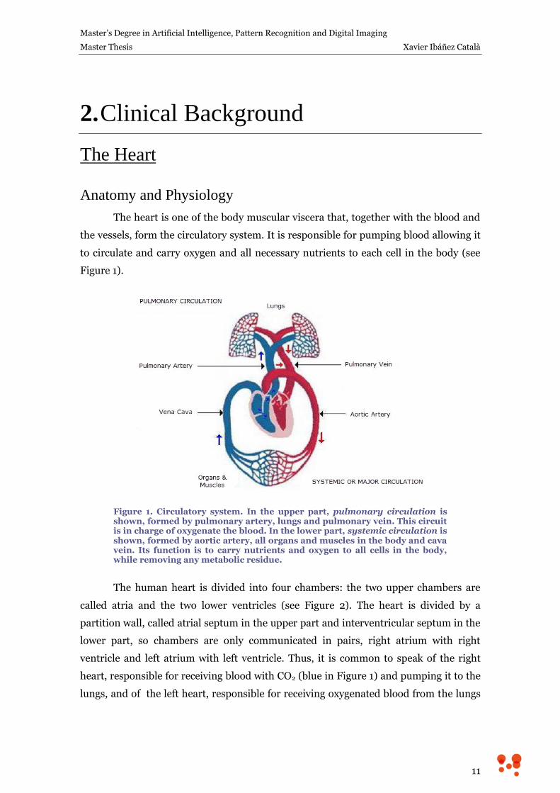
The heart is one of the body muscular viscera that, together with the blood and
the vessels, form the circulatory system. It is responsible for pumping blood allowing it
to circulate and carry oxygen and all necessary nutrients to each cell in the body (see
Figure 1).
Figure 1. Circulatory system. In the upper part, pulmonary circulation is shown, formed by pulmonary artery, lungs and pulmonary vein. This circuit is in charge of oxygenate the blood. In the lower part, systemic circulation is shown, formed by aortic artery, all organs and muscles in the body and cava vein. Its function is to carry nutrients and oxygen to all cells in the body, while removing any metabolic residue.
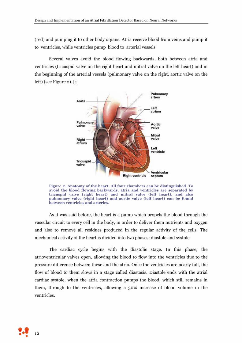
The human heart is divided into four chambers: the two upper chambers are
called atria and the two lower ventricles (see Figure 2). The heart is divided by a
partition wall, called atrial septum in the upper part and interventricular septum in the
lower part, so chambers are only communicated in pairs, right atrium with right
ventricle and left atrium with left ventricle. Thus, it is common to speak of the right
heart, responsible for receiving blood with CO2 (blue in Figure 1) and pumping it to the
lungs, and of the left heart, responsible for receiving oxygenated blood from the lungs
Design and Implementation of an Atrial Fibrillation Detector Based on Neural Networks
12
(red) and pumping it to other body organs. Atria receive blood from veins and pump it
to ventricles, while ventricles pump blood to arterial vessels.
Several valves avoid the blood flowing backwards, both between atria and
ventricles (tricuspid valve on the right heart and mitral valve on the left heart) and in
the beginning of the arterial vessels (pulmonary valve on the right, aortic valve on the
left) (see Figure 2). [1]
Figure 2. Anatomy of the heart. All four chambers can be distinguished. To avoid the blood flowing backwards, atria and ventricles are separated by tricuspid valve (right heart) and mitral valve (left heart), and also pulmonary valve (right heart) and aortic valve (left heart) can be found between ventricles and arteries.
As it was said before, the heart is a pump which propels the blood through the
vascular circuit to every cell in the body, in order to deliver them nutrients and oxygen
and also to remove all residues produced in the regular activity of the cells. The
mechanical activity of the heart is divided into two phases: diastole and systole.
The cardiac cycle begins with the diastolic stage. In this phase, the
atrioventricular valves open, allowing the blood to flow into the ventricles due to the
pressure difference between these and the atria. Once the ventricles are nearly full, the
flow of blood to them slows in a stage called diastasis. Diastole ends with the atrial
cardiac systole, when the atria contraction pumps the blood, which still remains in
them, through to the ventricles, allowing a 30% increase of blood volume in the
ventricles.
Master’s Degree in Artificial Intelligence, Pattern Recognition and Digital Imaging
Master Thesis Xavier Ibáñez Català
13
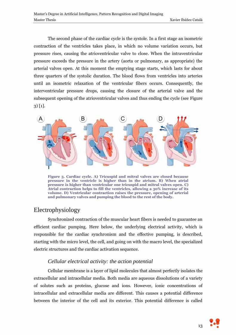
The second phase of the cardiac cycle is the systole. In a first stage an isometric
contraction of the ventricles takes place, in which no volume variation occurs, but
pressure rises, causing the atrioventricular valve to close. When the intraventricular
pressure exceeds the pressure in the artery (aorta or pulmonary, as appropriate) the
arterial valves open. At this moment the emptying stage starts, which lasts for about
three quarters of the systolic duration. The blood flows from ventricles into arteries
until an isometric relaxation of the ventricular fibers occurs. Consequently, the
interventricular pressure drops, causing the closure of the arterial valve and the
subsequent opening of the atrioventricular valves and thus ending the cycle (see Figure
3) [1].
Figure 3. Cardiac cycle. A) Tricuspid and mitral valves are closed because pressure in the ventricle is higher than in the atrium. B) When atrial pressure is higher than ventricular one tricuspid and mitral valves open. C) Atrial contraction helps to fill the ventricles, allowing a 30% increase of its volume. D) Ventricular contraction raises the pressure, opening of arterial and pulmonary valves and pumping the blood to the rest of the body.
Electrophysiology
Synchronized contraction of the muscular heart fibers is needed to guarantee an
efficient cardiac pumping. Here below, the underlying electrical activity, which is
responsible for the cardiac synchronism and the effective pumping, is described,
starting with the micro level, the cell, and going on with the macro level, the specialized
electric structures and the cardiac activation sequence.
Cellular electrical activity: the action potential
Cellular membrane is a layer of lipid molecules that almost perfectly isolates the
extracellular and intracellular media. Both media are aqueous dissolutions of a variety
of solutes such as proteins, glucose and ions. However, ionic concentrations of
intracellular and extracellular media are different. This causes a potential difference
between the interior of the cell and its exterior. This potential difference is called
Design and Implementation of an Atrial Fibrillation Detector Based on Neural Networks
14
resting potential and, in cardiac cells, has a value of approximately -90 mV (being the
extracellular medium the reference).
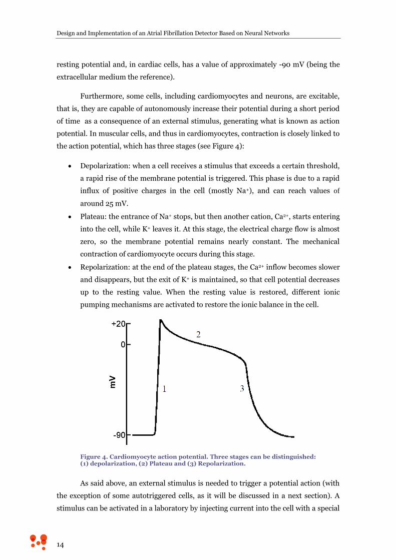
Furthermore, some cells, including cardiomyocytes and neurons, are excitable,
that is, they are capable of autonomously increase their potential during a short period
of time as a consequence of an external stimulus, generating what is known as action
potential. In muscular cells, and thus in cardiomyocytes, contraction is closely linked to
the action potential, which has three stages (see Figure 4):
Depolarization: when a cell receives a stimulus that exceeds a certain threshold,
a rapid rise of the membrane potential is triggered. This phase is due to a rapid
influx of positive charges in the cell (mostly Na+), and can reach values of
around 25 mV.
Plateau: the entrance of Na+ stops, but then another cation, Ca2+, starts entering
into the cell, while K+ leaves it. At this stage, the electrical charge flow is almost
zero, so the membrane potential remains nearly constant. The mechanical
contraction of cardiomyocyte occurs during this stage.
Repolarization: at the end of the plateau stages, the Ca2+ inflow becomes slower
and disappears, but the exit of K+ is maintained, so that cell potential decreases
up to the resting value. When the resting value is restored, different ionic
pumping mechanisms are activated to restore the ionic balance in the cell.
Figure 4. Cardiomyocyte action potential. Three stages can be distinguished: (1) depolarization, (2) Plateau and (3) Repolarization.
As said above, an external stimulus is needed to trigger a potential action (with
the exception of some autotriggered cells, as it will be discussed in a next section). A
stimulus can be activated in a laboratory by injecting current into the cell with a special
Master’s Degree in Artificial Intelligence, Pattern Recognition and Digital Imaging
Master Thesis Xavier Ibáñez Català
15
electrode, but in the natural state the stimulus that triggers the action potential of a
cardiac cell comes from an adjacent cell. Cardiomyocytes are connected to their
neighbors by the so-called intercalated disks, which contain special channels (known as
gap junctions) that allow the exchange of ions between cells. Thus, when a cardiac cell
is depolarized, it stimulates the depolarization of its neighbors, spreading the electrical
stimulus across the myocardium in a short time, allowing this way a synchronous
contraction of the cardiac muscle [2].
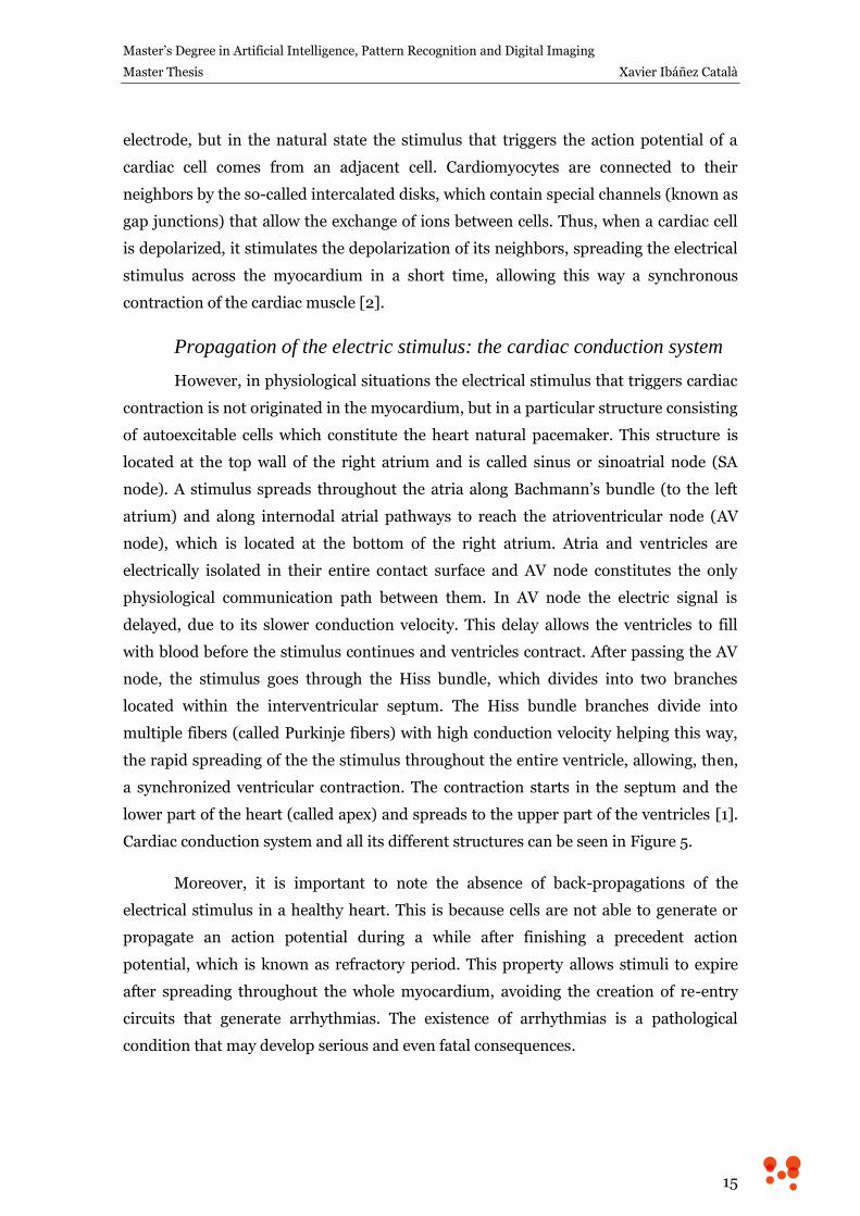
Propagation of the electric stimulus: the cardiac conduction system
However, in physiological situations the electrical stimulus that triggers cardiac
contraction is not originated in the myocardium, but in a particular structure consisting
of autoexcitable cells which constitute the heart natural pacemaker. This structure is
located at the top wall of the right atrium and is called sinus or sinoatrial node (SA
node). A stimulus spreads throughout the atria along Bachmann’s bundle (to the left
atrium) and along internodal atrial pathways to reach the atrioventricular node (AV
node), which is located at the bottom of the right atrium. Atria and ventricles are
electrically isolated in their entire contact surface and AV node constitutes the only
physiological communication path between them. In AV node the electric signal is
delayed, due to its slower conduction velocity. This delay allows the ventricles to fill
with blood before the stimulus continues and ventricles contract. After passing the AV
node, the stimulus goes through the Hiss bundle, which divides into two branches
located within the interventricular septum. The Hiss bundle branches divide into
multiple fibers (called Purkinje fibers) with high conduction velocity helping this way,
the rapid spreading of the the stimulus throughout the entire ventricle, allowing, then,
a synchronized ventricular contraction. The contraction starts in the septum and the
lower part of the heart (called apex) and spreads to the upper part of the ventricles [1].
Cardiac conduction system and all its different structures can be seen in Figure 5.
Moreover, it is important to note the absence of back-propagations of the
electrical stimulus in a healthy heart. This is because cells are not able to generate or
propagate an action potential during a while after finishing a precedent action
potential, which is known as refractory period. This property allows stimuli to expire
after spreading throughout the whole myocardium, avoiding the creation of re-entry
circuits that generate arrhythmias. The existence of arrhythmias is a pathological
condition that may develop serious and even fatal consequences.
Design and Implementation of an Atrial Fibrillation Detector Based on Neural Networks
16
Figure 5. Cardiac conduction system. Electrical stimulus is originated in SA node, and propagated throughout the atrium along Bachmann’s bundle and intermodal tracts. When reaching AV node, the stimulus is delayed and then propagated through the Hiss bundle to activate the ventricles in a down-top sequence.
Electrocardiography
Corporal fluids and organs surrounding the heart inside the chest are good
electric conductors, so depolarization waves spreading throughout the myocardium
generate electrical current flows across the chest. These current flows generate
electrical potential differences that can be measured on the body surface. The recording
of the heart electrical activity by using electrodes placed on a patient’s body is called
electrocardiography, and the voltage versus time signal resulting from this process is
referred to as an electrocardiogram (ECG). Electrical cardiac activity is a 3D process, so
different electrode locations will generate different points of view of the cardiac activity.
Each different point of view is known as a cardiac lead.
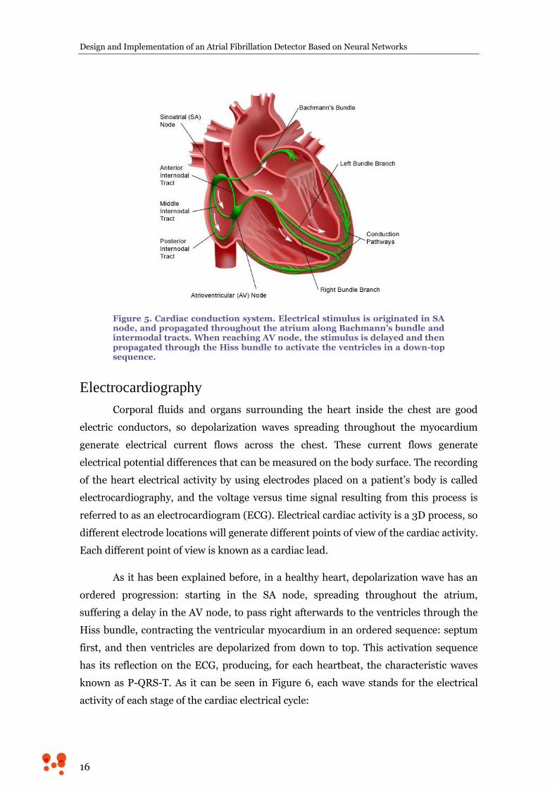
As it has been explained before, in a healthy heart, depolarization wave has an
ordered progression: starting in the SA node, spreading throughout the atrium,
suffering a delay in the AV node, to pass right afterwards to the ventricles through the
Hiss bundle, contracting the ventricular myocardium in an ordered sequence: septum
first, and then ventricles are depolarized from down to top. This activation sequence
has its reflection on the ECG, producing, for each heartbeat, the characteristic waves
known as P-QRS-T. As it can be seen in Figure 6, each wave stands for the electrical
activity of each stage of the cardiac electrical cycle:
Master’s Degree in Artificial Intelligence, Pattern Recognition and Digital Imaging
Master Thesis Xavier Ibáñez Català
17
P wave: represents the atrial depolarization.
PQ segment: is the period between the end of the P wave and the beginning of
the QRS complex. It represents the delay of the electrical stimulus in the AV
node and, as no myocardium is activating at that moment, the PQ segment is
flat. A shortening or enlarging of this segment may indicate conduction
problems in the AV node.
QRS complex: represents the sequential activation of the ventricles. Q wave
stands for the septum contraction, R wave for the lower part of the ventricles
and S wave for the upper part. An enlarging of the QRS duration may indicate
problems in the conduction of the Hiss bundle or its branches.
ST segment: is the period between the end of the S wave and the beginning of
the T wave. During the ST segment, all ventricular myocytes are contracted and
no electrical currents occur, so this segment is flat. An elevation or depression of
the ST may indicate myocardial infarction or ionic imbalance.
T wave: represents the repolarization and the consequent relaxation of the
ventricular myocardium.
Figure 6. ECG waves [3]. Each wave of the P-QRS-T complex is related to the electrical activity of different cardiac structures. P wave: atrial depolarization. PQ segment: delay in the AV node. QRS wave: ventricular depolarization. ST segment: time during ventricular myocardium is contracted. T wave: ventricular repolarization.
Design and Implementation of an Atrial Fibrillation Detector Based on Neural Networks
18
Atrial Fibrillation
Atrial fibrillation (AF) is a fast arrhythmia (tachyarrhythmia) characterized by
the set up of recurrent, multiple and uncoordinated electrical waves in the atrium that
excite the atrial myocardium in a totally disorganized way. As a result, atrial
contraction is inexistent, indeed, and instead of contracting, atrial tissue just vibrates.
This has two consequences: on the one hand, the absence of atrial contraction
decreases the heart beating efficiency by a 20 to 30%; on the other, the existence of
erratic and recurrent activation waves in the atrium triggers arrhythmic, uncoordinated
and usually fast, ventricular beats [1].
AF usually progresses from short, rare episodes, to longer and more frequent
attacks. Clinically, different types of AF are distinguished, based on the presentation
and duration of the arrhythmia [4]:
Paroxysmal AF consists of self-terminating episodes, usually shorter than
48h.
Persistent AF is present when an AF episode either lasts longer than 7 days or
requires termination by cardioversion (either pharmacological or electrical).
Long-standing persistent AF is considered so when it has lasted for more
than 1 year.
Permanent AF is said to exist when the presence of the arrhythmia is accepted
both by the patient and the physician.
In general terms, a patient is usually diagnosed from paroxysmal AF and as time
goes on it will evolve to sustained forms of AF. The distribution of paroxysmal AF
recurrences is not random, but clustered, and AF burden (the time ratio with and
without AF) can vary markedly over months or even years in individual patients.
Asymptomatic AF (silent AF) is common even in symptomatic patients, irrespective of
whether the initial presentation was persistent or paroxysmal.
Epidemiology and Related Pathologies
AF is the most common sustained arrhythmia, affecting 1–2% of the population.
Over 6 million Europeans suffer from this arrhythmia, and its prevalence is estimated
to, at least, double in the next 50 years as the population ages. AF prevalence increases
with age, from 0.5% at 40–50 years, to 5–15% at 80 years. Men are more often affected
Master’s Degree in Artificial Intelligence, Pattern Recognition and Digital Imaging
Master Thesis Xavier Ibáñez Català
19
than women. The lifetime risk of developing AF is ~25% in those who have reached the
age of 40 [4].
As atrial beat is inexistent during AF, blood flows passively to the ventricles,
which can generate regions inside the atrium where blood hardly moves, causing the
blood to coagulate, which can produce stroke and other thrombo-embolic events. In
fact, AF confers 5-fold risk of stroke, and one in five of all strokes is attributed to this
arrhythmia. Paroxysmal AF carries the same stroke risk as permanent or persistent AF,
since AF episodes of few hours of duration are enough for thrombus formation.
Ischemic strokes in association with AF are often fatal, and those patients who survive
are left more disabled by their stroke and more likely to suffer a recurrence than
patients with other causes of stroke. In addition to that, as a result of the irregular, fast
ventricular rate, patients with AF have significantly poorer quality of life, and their
exercise capacity is considerably reduced [4][5].
Symptoms and Diagnosis
Many patients with AF have no symptoms (silent AF), which makes that many
of them remain undiagnosed, even an important amount of them will never present to
hospital. In fact, many patients are firstly diagnosed of silent AF after suffering a
cryptogenic stroke. When symptomatic, patients with AF suffer from palpitations,
irregular and rapid heartbeat, fatigue (general or when exercised), faintness or
confusion, dizziness or shortness of breath, among others.
An irregular pulse should always raise the suspicion of AF, but an ECG
recording with at least 30 seconds duration must be done to differentiate AF from other
supraventricular or ventricular arrhythmias. In an ECG recording, AF shows irregular
narrow beats (supraventricular origin) and indistinguishable P wave, although some
low amplitude noisy activity can be observed in the base line (especially in those leads
that have good representation of atrial activity, as V1). As an example, in panel A) of
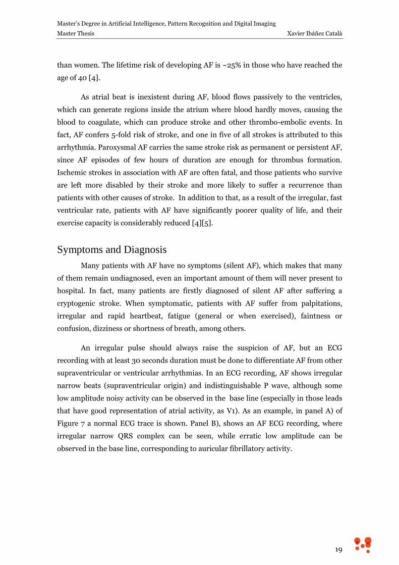
Figure 7 a normal ECG trace is shown. Panel B), shows an AF ECG recording, where
irregular narrow QRS complex can be seen, while erratic low amplitude can be
observed in the base line, corresponding to auricular fibrillatory activity.
Design and Implementation of an Atrial Fibrillation Detector Based on Neural Networks
20
Figure 7. Normal and AF ECG. A) normal ECG trace. B) AF ECG trace, where irregular narrow QRS complexes can be seen, while erratic low amplitude can be observed in the base line, corresponding to auricular fibrillatory activity.
As mentioned above, AF episodes can self-terminate and the triggering
situations of a new episode are not easily predictable. Thus, only an opportunistic ECG
could find the arrhythmia. Moreover, assessment of the AF burden is important to
decide the treatment or to evaluate the effectiveness of a therapy [6]. It has been
estimated that 7 day Holter ECG recording or daily and symptom-activated event
recordings may document the arrhythmia in approximately 70% of AF patients, and
that their negative predictive value for the absence of AF is between 30 and 50% [7].
For that reason, long term (24h to 7 days) ambulatory ECG monitoring is
recommended for diagnosing and controlling the evolution of patients with AF; even, in
highly symptomatic patients longer monitoring times should be evaluated, including
the implantation of a cardiac monitor which allows over 2 year monitoring [4][5].
Different technical alternatives for long term cardiac monitoring will be carefully
discussed in the next chapter.
Master’s Degree in Artificial Intelligence, Pattern Recognition and Digital Imaging
Master Thesis Xavier Ibáñez Català
21
3. Technical Background and State of
the Art
Ambulatory ECG Monitoring
Ambulatory ECG monitoring is a widely used noninvasive technique in which
ECG is continuously recorded over an extended period of time, typically 24 to 48 hours,
to evaluate symptoms suggestive of cardiac arrhythmias, i.e., palpitations, dizziness, or
syncope. Norman J. Holter was the first one to introduce the ambulatory ECG
monitoring in the 1940s, for that reason, the ECG recording of ambulatory patients is
nowadays known as Holter test. The original Holter monitor was a 35 kg backpack with
a reel-to-reel FM tape recorder, analog patient interface electronics and large and heavy
batteries which enabled it to record a single ECG lead during several hours.[8]
Traditional Holter Test
From Norman Holter’s time up to now, ambulatory ECG recorders have been
gradually modified to incorporate several technological enhancements. If first Holter
recorder was a 35 kg backpack with a reel-to-reel FM tape recorder, in the 1990s they
had the size of a walkman and recorded the ECG on a cassette tape, and nowadays they
use flashcard memory, digital electronics and their size is so reduced that they are
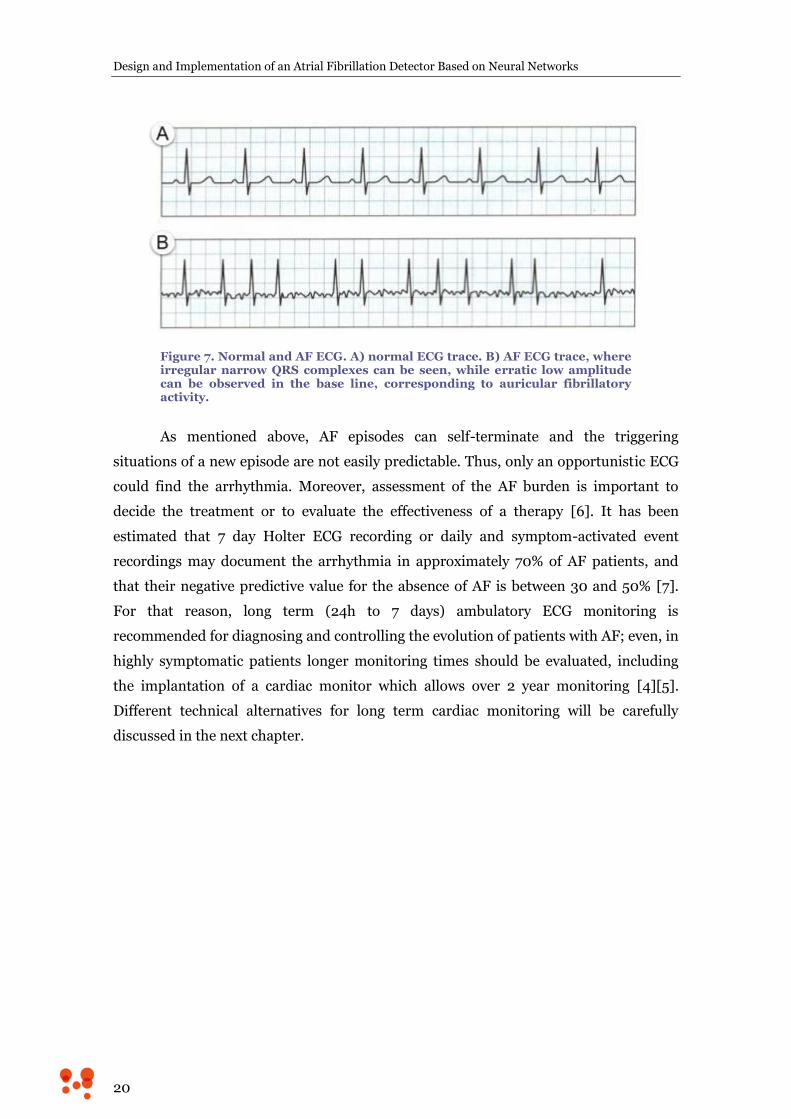
slightly bigger than the AAA battery that they need to work. Figure 8 shows the
technological evolution of Holter systems over the last decades. Holter recorders often
include an event button for the patient to indicate the presence of symptoms or any
other remarkable event. Once the monitor is returned, data are analyzed and correlated
with marked events and symptoms.
Although technological advances have reduced size and weight of monitors, and
have eased the whole process of recording and processing the signals, the medical test
known as Holter has not experienced any change for a long time. It is defined as an,
ideally, three lead ambulatory ECG recording, during at least 24h and no more than
48h, using adhesive and disposable electrodes wired to the recorder. [9]
One limitation of traditional Holter systems comes from the use of adhesive
electrodes, which can produce allergic reactions, and wires, that may introduce noise in
ECG signal when moved (and patient is expected to move in his/her daily life), so ECG
Design and Implementation of an Atrial Fibrillation Detector Based on Neural Networks
22
signal can be very noisy in active patients. But the main limitation is that Holter
monitoring has been demonstrated to have reduced diagnostic yield [10][11], so it will
be ineffective when patients experience infrequent symptoms or pathologic events. For
that reason, clinical guidelines are encouraging doctors to perform longer monitoring
than 24h [9], at least 7 days to achieve a good diagnostic yield for AF [7], and even
more if symptoms are infrequent.
Figure 8. Evolution of Holter devices over last decades. A) Model 445 Mini-Holter Recorder, released in 1976. B) RZ151 Series Cassette Holter, released in late 1990s. C) Mortara H3+, currently on market.
Long-Term Cardiac Monitoring
Since traditional 24h Holter has limited diagnostic yield and it is proved that
longer monitoring times improve the diagnostic yield [10][11], many strategies have
been developed to extend monitoring times. This section will analyze each strategy and
present some representative products.
Ambulatory Event Monitor
Ambulatory event monitors (AEMs) were developed to provide longer periods of
monitoring than a regular Holter. They are attached to the patient by chest electrodes
and they record ECG whenever activated by the patient (by pressing an event button
Master’s Degree in Artificial Intelligence, Pattern Recognition and Digital Imaging
Master Thesis Xavier Ibáñez Català
23
when any symptom is felt). Some of these devices are continuously monitoring (but not
recording) the cardiac rhythm and, if a slow, fast or irregular heart rate is detected, an
activation is triggered. Once activated, data are stored for a programmable fixed
amount of time before the activation and a period of time after the activation.
Another less sophisticated form of event monitor is the post-event recorder.
This one is not worn continuously but instead it is applied directly to the chest area
once a symptom develops, so it cannot record the rhythm before the device is activated.
Both event monitors and post-event recorders usually have a looping memory.
This means that the newest event will erase the oldest when memory is fully written.
For this reason, these devices are also referred as event loop recorders (ELRs).
The limitations of these devices include the following. On the one hand, the
patient has to be awake and coherent enough to activate the device, unless automatic
event detection is build into the monitor and the automatic algorithm detects the
cardiac event. On the other hand, a significant percentage of patients are noncompliant
with continuous application of the devices, mostly because the skin is irritated or
damaged by the electrodes and also because of poor quality signal during exercise.
Finally, what maybe the most important limitation is that, in automatically triggered
devices, the memory can be filled up with noisy signals as a result of false positive
detections, erasing any true event recorded in the past.[8][9]
Holter Patch
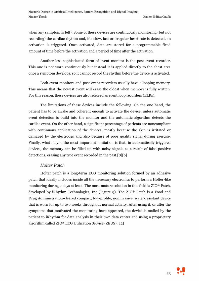
Holter patch is a long-term ECG monitoring solution formed by an adhesive
patch that ideally includes inside all the necessary electronics to perform a Holter-like
monitoring during 7 days at least. The most mature solution in this field is ZIO® Patch,
developed by iRhythm Technologies, Inc (Figure 9). The ZIO® Patch is a Food and
Drug Administration-cleared compact, low-profile, noninvasive, water-resistant device
that is worn for up to two weeks throughout normal activity. After using it, or after the
symptoms that motivated the monitoring have appeared, the device is mailed by the
patient to iRhythm for data analysis in their own data center and using a proprietary
algorithm called ZIO® ECG Utilization Service (ZEUS).[12]
Design and Implementation of an Atrial Fibrillation Detector Based on Neural Networks
24
Figure 9. ZIO® XT Patch, by iRhythm Technologies, Inc.
iRhythm and other patch manufacturers have made a great effort in electronics
miniaturization and autonomy optimization, and, of course, in developing
hypoallergenic adhesives with embedded wet gel electrodes able to last up to 14 days on
the skin enduring movements, sweat and water. However, it is a challenge partially
achieved attending to the work of Turakhia et al. [11], where a population of 26,751
wearing ZIO® Patch was studied and the result was that 50% of the patches were only
worn until day 7, and 75% until day 10 of monitoring.
Smart Fabric Holter – NUUBO
Nuubo is a Spanish SME-medical device company founded in 2005, and it
focuses on cardiac monitoring solutions based on wearable medical technologies (smart
fabrics), targeting the medical and sport medicine global markets.
Nuubo ECG Wearable Cardiac Monitoring System is a complete and non-
invasive solution for monitoring and analysing cardiac and physical activity of an
individual or group by using a biomedical garment, an electronic device and a software
analysis. Nuubo’s technology is based on a garment comprising a sensor with flexibility
and elasticity, which allows recording good quality ECG signals, even in movement,
with improved adhesion properties but avoiding adhesive elements which produce skin
irritations.
BlendFix® Sensor Electrode Technology is the core sensor technology that is
based on the use of flexible and elastic electrically conductive silicone materials
integrated into elastomeric polymer wearable sensors “printed” into a garment for
everyday use. Nuubo’s core sensor technology main benefits are:
Optimal ECG signal quality both during regular activities and sport practice.
Easy-to-use: it does not need supervised placement, because electrodes are
placed on an easy to vest wearable.
Master’s Degree in Artificial Intelligence, Pattern Recognition and Digital Imaging
Master Thesis Xavier Ibáñez Català
25
Comfortable: elasticity drives both comfort and adaptability to the normal
thoracic chamber movements, enabling the patients to comfortably perform real
day-to-day activities and sports specially.
Sensing versatility: electrodes can be printed onto almost any textile, and in any
form or size.
Very low manufacturing cost.
Nuubo has received CE-Mark approval for the commercial sale of both single-
lead and multi-lead solution. These product solutions are compliant with Medical
Device Directive 93/42/EEC, and the company is also certified as a medical device
company by ISO 9001 and ISO 13485.
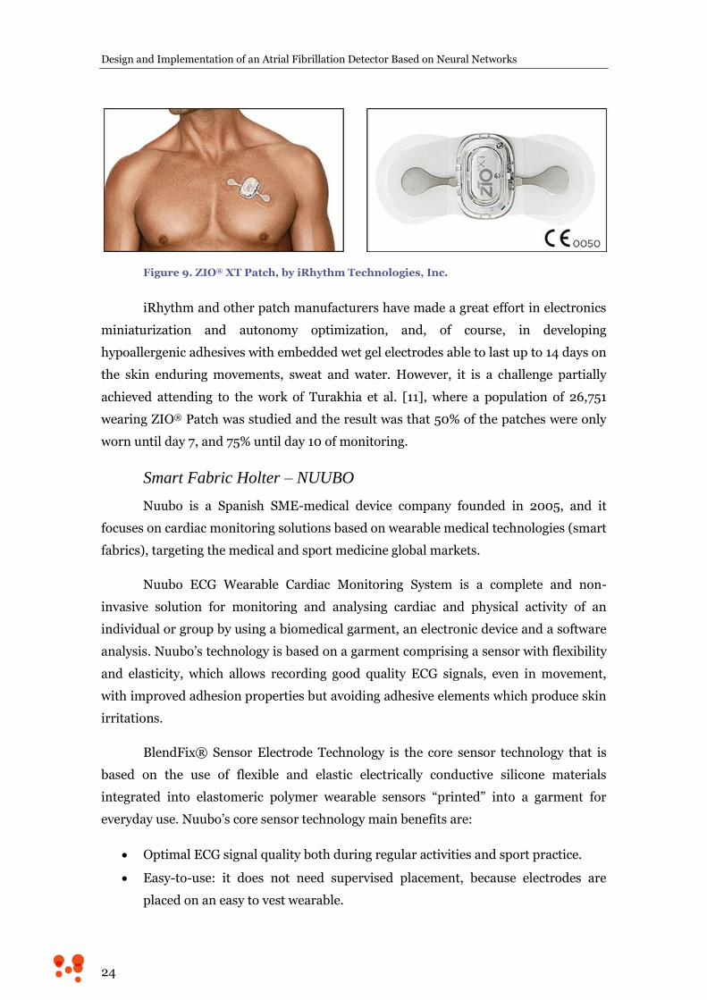
Nuubo’s portfolio offers different solutions to cover the ECG monitoring from 7
to 60 days, both for regular and sportive activity, using 1 or 3 leads. Nuubo’s products
have been proved to achieve high patient’s compliance with ECG signal of excellent
quality [13][14] and to be of great utility in sport medicine [15][16]. In Figure 10 a
sample of Nuubo’s portfolio is shown.
Figure 10. Sample of Nuubo’s portfolio. A) 1 lead wearable, designed for longer than 4 weeks monitoring. B and C) Two concepts of 3 lead wearable, for 1 or 4 weeks respectively. D) 3 lead wearable specially designed for sportive activity. E) 3 lead wearable conceived for pediatrics monitoring.
Mobile Cardiac Telemetry
Mobile Cardiac Telemetry (MCT) refers to a concept that comprises all the
systems involved in a real-time continuous attended cardiac monitoring service. MCT is
designed to combine the benefits and avoid the limitations of Holter monitors and
standard ELRs.
They are worn continuously and are similar in size to the standard ELR. They
continuously record the ECG signal of ambulatory patients and automatically generate
and transmit an arrhythmic event. Those events can be patient or event-activated.
Events are transmitted usually to a secondary device which communicates by cellular
Design and Implementation of an Atrial Fibrillation Detector Based on Neural Networks
26
phone network with a monitoring station, where trained staff members analyze live
incoming patient’s data and inform the referring physician according to previously
defined criteria.[8]
For example, CardioNet Inc. is a company that offers mobile cardiac outpatient
telemetry. In this system, called Mobile Cardiac Outpatient TelemetryTM (MCOTTM),
the patient wears a 3-lead sensor, which constantly communicates with the MCOT
monitor, a lightweight unit that can be carried in a pocket or a purse. When an
arrhythmia is detected according to preset parameters, the ECG is automatically
transmitted to a central CardioNet service center, where the ECG is immediately
interpreted and results sent to the referring physician. The referring physician can
request the level and timing of response, ranging from daily reports to immediate
results.
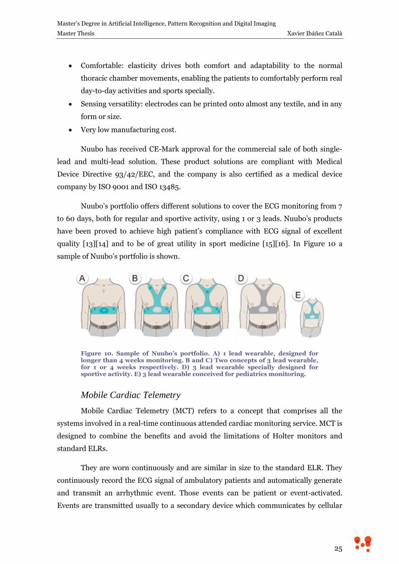
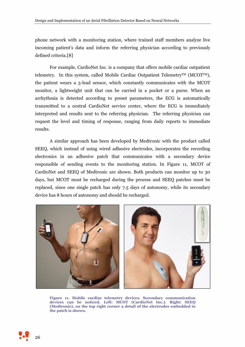
A similar approach has been developed by Medtronic with the product called
SEEQ, which instead of using wired adhesive electrodes, incorporates the recording
electronics in an adhesive patch that communicates with a secondary device
responsible of sending events to the monitoring station. In Figure 11, MCOT of
CardioNet and SEEQ of Medtronic are shown. Both products can monitor up to 30
days, but MCOT must be recharged during the process and SEEQ patches must be
replaced, since one single patch has only 7.5 days of autonomy, while its secondary
device has 8 hours of autonomy and should be recharged.
Figure 11. Mobile cardiac telemetry devices. Secondary communication devices can be noticed. Left: MCOT (CardioNet Inc.). Right: SEEQ (Medtronic), on the top right corner a detail of the electrodes embedded in the patch is shown.
Master’s Degree in Artificial Intelligence, Pattern Recognition and Digital Imaging
Master Thesis Xavier Ibáñez Català
27
Very Long-Term Cardiac Monitoring: Implantable Loop Recorder
Implantable Loop Recorders (ILRs) are implanted beneath the skin through a
small incision of about 2 cm in the left precordial region. They are equipped with a
looping memory and they are either automatically-triggered or patient-triggered by
using an external activator at the moment the symptoms arise. Once activated, they
record one-lead electrocardiographic trace for several minutes before and after the
event.
In general, monitoring lasts either until a diagnosis is reached or until the
battery runs down, which can last up to 36 months. When completion of monitoring is
achieved, the device is removed from the patient. The newest generation of these
devices allows remote transmission of data to a communication base which transmits
data to a monitoring center by using wired or cellular phone networks. Besides, many
pacemakers and implantable cardio-defibrillators incorporate this monitoring
functionality. [9]
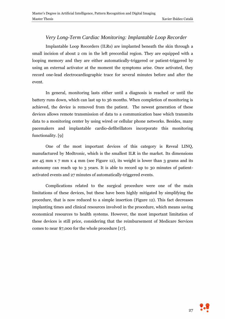
One of the most important devices of this category is Reveal LINQ,
manufactured by Medtronic, which is the smallest ILR in the market. Its dimensions
are 45 mm x 7 mm x 4 mm (see Figure 12), its weight is lower than 3 grams and its
autonomy can reach up to 3 years. It is able to record up to 30 minutes of patient-
activated events and 27 minutes of automatically-triggered events.
Complications related to the surgical procedure were one of the main
limitations of these devices, but these have been highly mitigated by simplifying the
procedure, that is now reduced to a simple insertion (Figure 12). This fact decreases
implanting times and clinical resources involved in the procedure, which means saving
economical resources to health systems. However, the most important limitation of
these devices is still price, considering that the reimbursement of Medicare Services
comes to near $7,000 for the whole procedure [17].
Design and Implementation of an Atrial Fibrillation Detector Based on Neural Networks
28
Figure 12. Reveal LINQ of Medtronic. Upper left, Reveal Linq is shown to appreciate its reduced size. Upper right, insertion tool is shown. Bottom, insertion procedure is shown.
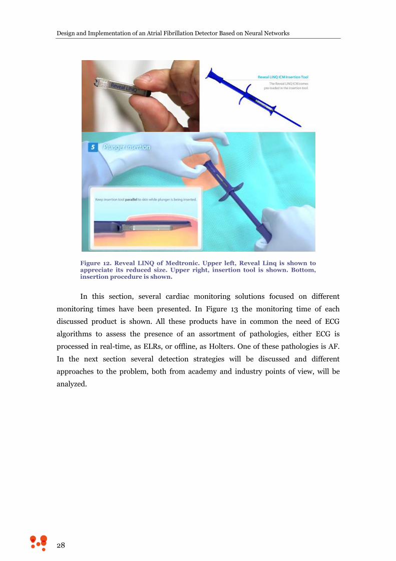
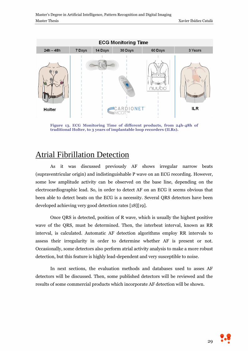
In this section, several cardiac monitoring solutions focused on different
monitoring times have been presented. In Figure 13 the monitoring time of each
discussed product is shown. All these products have in common the need of ECG
algorithms to assess the presence of an assortment of pathologies, either ECG is
processed in real-time, as ELRs, or offline, as Holters. One of these pathologies is AF.
In the next section several detection strategies will be discussed and different
approaches to the problem, both from academy and industry points of view, will be
analyzed.
Master’s Degree in Artificial Intelligence, Pattern Recognition and Digital Imaging
Master Thesis Xavier Ibáñez Català
29
Figure 13. ECG Monitoring Time of different products, from 24h-48h of traditional Holter, to 3 years of implantable loop recorders (ILRs).
Atrial Fibrillation Detection
As it was discussed previously AF shows irregular narrow beats
(supraventricular origin) and indistinguishable P wave on an ECG recording. However,
some low amplitude activity can be observed on the base line, depending on the
electrocardiographic lead. So, in order to detect AF on an ECG it seems obvious that
been able to detect beats on the ECG is a necessity. Several QRS detectors have been
developed achieving very good detection rates [18][19].
Once QRS is detected, position of R wave, which is usually the highest positive
wave of the QRS, must be determined. Then, the interbeat interval, known as RR
interval, is calculated. Automatic AF detection algorithms employ RR intervals to
assess their irregularity in order to determine whether AF is present or not.
Occasionally, some detectors also perform atrial activity analysis to make a more robust
detection, but this feature is highly lead-dependent and very susceptible to noise.
In next sections, the evaluation methods and databases used to asses AF
detectors will be discussed. Then, some published detectors will be reviewed and the
results of some commercial products which incorporate AF detection will be shown.
Design and Implementation of an Atrial Fibrillation Detector Based on Neural Networks
30
Evaluation of AF detectors
The evaluation of AF detectors is a controversial topic. Several results have been
published using private databases, which make results impossible to reproduce. In
addition to that, different evaluation methods are used to assess the performance of the
detectors, as per patient detection or elimination from the statistics of those episodes
shorter than the evaluation interval used by the detector. Consider [20], [21] and [22]
as a brief sample.
When public databases are used, MIT-BIH Arrhythmia Database and MIT-BIH
Atrial Fibrillation Database are commonly employed. Both are described below.
MIT-BIH Arrhythmia Database
MIT-BIH Arrhythmia Database (MITDB from this point on) is a widely used
public database which is freely available from PhysioNet [23], and comprises 48 fully
annotated records. Annotations were done by two independent cardiologists, and when
any discrepancy was found, it was solved by consensus. Annotations comprise beat
annotations with its position and type label, and also rhythm labels, signal quality
labels, and comments.
The source of the ECGs included in the MITDB is a set of over 4000 long-term
Holter recordings that were obtained by the Beth Israel Hospital Arrhythmia
Laboratory between 1975 and 1979. The database contains 23 records (numbered from
100 to 124 inclusive with some numbers missing) chosen at random from this set, and
25 records (numbered from 200 to 234 inclusive, again with some numbers missing)
selected from the same set to include a variety of rare but clinically important
phenomena that would not be well-represented by a small random sample of Holter
recordings. Each of the 48 records is slightly over 30 minutes long.
The first group is intended to serve as a representative sample of the variety of
waveforms and artifact that an arrhythmia detector might encounter in routine clinical
use. The records in the second group were chosen to include complex ventricular,
junctional, and supraventricular arrhythmias and conduction abnormalities. Several of
these records were selected because features of the rhythm, QRS morphology variation,
or signal quality may be expected to present significant difficulty to arrhythmia
detectors. [24]
Attending to AF, only 7 records of MITDB contain paroxysmal AF, and all
episodes totalized count 1 hour and 43 minutes. Besides, different kinds of complex
Master’s Degree in Artificial Intelligence, Pattern Recognition and Digital Imaging
Master Thesis Xavier Ibáñez Català
31
pathologic rhythms are included in MITDB, which joined to the low prevalence, make it
a difficult database to test AF.
MIT-BIH Atrial Fibrillation Database
Firstly developed for [25], MIT-BIH Atrial Fibrillation Database (AFDB from
this point on) is formed by 23 records of 10 hours of duration, selected from a library of
over 8000 24 hours Holter recordings collected by the Arrhythmia Laboratory of Beth
Israel Hospital. A total of 93 hours of AF is contained in AFDB, mostly paroxysmal
episodes.
Only AF, atrial flutter, junctional flutter and normal rhythm (used to indicate all
other rhythms) are labeled. Besides, two beat annotation files were prepared. First file
was prepared using an automated QRS detector without correcting the results, which
may be useful for studies of methods of automated AF detection where such methods
must be robust with respect to typical QRS detection errors. Second file includes
manually corrected beat annotations, which may be preferred for basic studies of AF
itself, where QRS detection errors would be confounding. Both beat annotation files
only contain the position of the R peak of the QRS, but beats are not classified by types.
Academic Solutions
In this section a review through several published AF detectors is shown. Only
those algorithms showing results on MITDB or AFDB have been selected. Table 1 shows
a comparative study of the results. Brief description of each algorithm is provided
below.
Moody et al [25] employ a hidden Markov model (HMM) to represent an RR
interval sequence using three states: short, normal or long with respect to a sliding
average. The HMM was trained using a subset of MITDB selected to contain AF,
normal sinus rhythm and other rhythms considered likely to confuse an AF detector. It
was tested on AFDB, originally created for this publication.
Artis et al [26] use the three-state modeling employed by Moody in [25] to feed
an artificial neural network (ANN) to classify a segment of RR intervals into AF or no
AF categories. After that, a sliding averaging postprocessing is performed to detect
transitions. It was trained and tested using the same databases as Moody in [25].
Young et al. [27] use a HMM with 2 states (AF or no AF) with a sequence of 3
RR intervals classified in 7 categories, in a similar way as Moody did in [25]. HMM
Design and Implementation of an Atrial Fibrillation Detector Based on Neural Networks
32
output is a low pass filtered to make delineation of AF episodes easier. The algorithm
was trained and tested using the same databases as Moody did in [25].
Tatento and Glass, in 2000 [28], proposed an algorithm that used the
Kolmogorov-Smirnov (KS) test to assess the irregularity of ΔRR (difference between
consecutive RR intervals) calculated on a sequence of 100 consecutive beats. AFDB was
used to train the algorithm and a subset of MITDB (containing only the signals with
AF) was used for test. One year after, they published a more detailed and depurated
version of the algorithm [29], that was tested on full MITDB and obtained better results
than in the first one.
Ghodrati and Marinello [30] proposed in 2008 a method based on modeling the
RR interval as both Gaussian and Laplace probability density function, and then
applying Neyman-Pearson detection criteria. MITDB was used for training and AFDB
for testing.
Couceiro et al. [31] used an artificial neural network classifier which received
three inputs: RR irregularity assessment based in HMM in a similar way to Moody’s in
[25], ratio of detected P waves and spectral analysis of the atrial activity after
performing QRS-T cancellation. A subset of AFDB was used to train the algorithm and
complete AFDB was used for testing.
Sarkar et al. [32] proposed a computationally simple AF detector based on
statistical analysis of the histogram of the Lorentz plot of ΔRR. They used an AFDB
subset and a private database to search the thresholds that optimized the area under
curve (AUC) ROC (Receiver Operating Curve). It was tested on full AFDB, MIT-BIH
Normal Sinus Rhythm Database (NSRDB), Normal Sinus Rhythm RR Interval
Database (NSRDB_RR) from Physionet and other private databases.
In 2009, Dash et al. [33] developed a detector based on a statistical approach.
Their detector calculates turning points ratio, root mean square of successive
differences and Shannon entropy of 128 consecutive RR intervals. Thresholds were
found by maximizing AUC. They used AFDB and MITDB both for testing and training
the algorithm.
In the same year, Babaeizadeh et al. [34] published a detector that uses HMM to
produce an AF score that is enhanced by adding atrial activity analysis. They used
private database to develop the algorithm and they tested it on AFDB.
Master’s Degree in Artificial Intelligence, Pattern Recognition and Digital Imaging
Master Thesis Xavier Ibáñez Català
33
Huang et al. [35] proposed an algorithm to detect transitions between AF and
sinus rhythm by using a statistical analysis based on KS test of the preprocessed ΔRR
sequence. AFDB and other private database were used to train, and NSRDB and private
database to test.
Lian et al. [36] developed method is based on counting non null bins of the
histogram of RR vs. ΔRR. They used AFDB, NSRDB, NSRDB_RR and MIT-BIH Long
Term Atrial Fibrillation Database (LTAFDB) to find the threshold that maximizes AUC,
and tested on the same databases.
Zhou et al. [37] published last year an interesting approach that assesses the
irregularity of RR by using the entropy of symbolic dynamics of the sequence. For this,
after preprocessing, ΔRR is transformed to ten different symbols and 3-symbol words
are then analyzed to detect transitions between AF and other rhythms. LTAFDB was
used to train and AFDB, MITDB and NSRDB were used to test.
And finally, this year, Petrėnas et al. [38] presented a low-complexity detector
based on statistical analysis of RR sequence. An ectopic correction method is
incorporated and short windows of 8 beats are used to detect transitions. LTAFDB was
used to train and AFDB, and NSRDB were used to test.
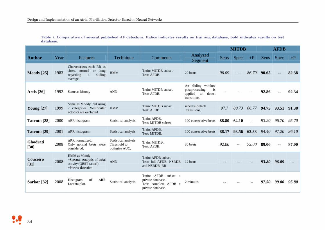
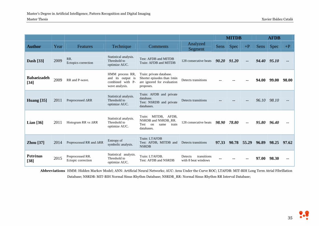
Results and other details of each algorithm can be found in Table 1. Observe
that results in italics have been obtained using training database and bold results have
been obtained using test database.
Design and Implementation of an Atrial Fibrillation Detector Based on Neural Networks
34
Table 1. Comparative of several published AF detectors. Italics indicates results on training database, bold indicates results on test database.
MITDB AFDB
Author Year Features Technique Comments Analyzed
Segment Sens Spec +P Sens Spec +P
Moody [25] 1983
Characterizes each RR as
short, normal or long
regarding a sliding
average.
HMM Train: MITDB subset.
Test: AFDB. 20 beats 96.09 -- 86.79 90.65 -- 82.38
Artis [26] 1992 Same as Moody ANN Train: MITDB subset.
Test: AFDB.
An sliding window
postprocessing is
applied to detect
transitions.
-- -- -- 92.86 -- 92.34
Young [27] 1999 Same as Moody, but using
7 categories. Ventricular
ectopics are excluded.
HMM Train: MITDB subset.
Test: AFDB.
4 beats (detects
transitions) 97.7 88.73 86.77 94.75 93.51 91.38
Tatento [28] 2000 ΔRR histogram Statistical analysis Train: AFDB.
Test: MITDB subset 100 consecutive beats 88.80 64.10 -- 93.20 96.70 95.20
Tatento [29] 2001 ΔRR histogram Statistical analysis Train: AFDB.
Test: MITDB. 100 consecutive beats 88.17 93.56 62.33 94.40 97.20 96.10
Ghodrati
[30] 2008
ΔRR normalized.
Only normal beats were
considered.
Statistical analysis.
Threshold to
optimize AUC.
Train: MITDB.
Test: AFDB. 30 beats 92.00 -- 73.00 89.00 -- 87.00
Couceiro
[31] 2008
HMM as Moody
+Spectral Analysis of atrial
activity (QRST cancel)
+P wave detection
ANN
Train: AFDB subset.
Test: full AFDB, NSRDB
and NSRDB_RR
12 beats -- -- -- 93.80 96.09 --
Sarkar [32] 2008 Histogram of ΔRR
Lorentz plot. Statistical analysis
Train: AFDB subset +
prívate database.
Test: complete AFDB +
prívate database.
2 minutes -- -- -- 97.50 99.00 95.80
Master’s Degree in Artificial Intelligence, Pattern Recognition and Digital Imaging
Master Thesis Xavier Ibáñez Català
35
MITDB AFDB
Author Year Features Technique Comments Analyzed
Segment Sens Spec +P Sens Spec +P
Dash [33] 2009 RR.
Ectopics correction
Statistical analysis.
Threshold to
optimize AUC.
Test: AFDB and MITDB
Train: AFDB and MITDB 128 consecutive beats 90.20 91.20 -- 94.40 95.10 --
Babaeizadeh
[34] 2009 RR and P-wave.
HMM process RR,
and its output is
combined with P-
wave analysis.
Train: private database.
Shorter episodes than 1min
are ignored for evaluation
proposes.
Detects transitions -- -- -- 94.00 99.00 98.00
Huang [35] 2011 Preprocessed ΔRR
Statistical analysis.
Threshold to
optimize AUC.
Train: AFDB and private
database.
Test: NSRDB and private
databases.
Detects transitions -- -- -- 96.10 98.10 --
Lian [36] 2011 Histogram RR vs ΔRR
Statistical analysis.
Threshold to
optimize AUC.
Train: MITDB, AFDB,
NSRDB and NSRDB_RR.
Test on same train
databases.
128 consecutive beats 98.90 78.80 -- 95.80 96.40 --
Zhou [37] 2014 Preprocessed RR and ΔRR Entropy of
symbolic analysis.
Train: LTAFDB
Test: AFDB, MITDB and
NSRDB
Detects transitions 97.33 90.78 55.29 96.89 98.25 97.62
Petrėnas
[38] 2015
Preprocessed RR.
Ectopic correction
Statistical analysis.
Threshold to
optimize AUC.
Train: LTAFDB.
Test: AFDB and NSRDB Detects transitions
with 8 beat windows -- -- -- 97.00 98.30 --
Abbreviations HMM: Hidden Markov Model; ANN: Artificial Neural Networks; AUC: Area Under the Curve ROC; LTAFDB: MIT-BIH Long Term Atrial Fibrillation
Database; NSRDB: MIT-BIH Normal Sinus Rhythm Database; NSRDB_RR: Normal Sinus Rhythm RR Interval Database;
Design and Implementation of an Atrial Fibrillation Detector Based on Neural Networks
36
To sum up, several AF detection algorithms have been discussed. They use
different approaches to analyze RR irregularity, as HMM, ANN, statistical analysis or
symbolic dynamics analysis. Some of them perform ectopic correction to remove
irregularity sources that can be confused with AF irregularity. Also, some other
methods use atrial activity assessment to add more information to the RR irregularity
evaluation in order to make more informed decisions. However, results are not better
than those obtained without using it.
First detectors, especially those detectors inspired in Moody’s [25]
methodology, commonly employ MITDB to train the algorithms and AFDB to test.
Detectors using MITDB as test database have quite low positive predictivity, while
those using AFDB as test database have higher statistics, clearly showing that MITDB is
a more difficult database for an AF detector than AFDB one, as discussed in previous
sections. In addition to that, using the same databases for training and testing is a
recurrent methodological mistake.
Industrial Solutions
Regulations and Standards
In general, commercial products must comply with several standards to ensure
that their essential workings fulfill some specific features that make the product safe for
the expected use. This fact becomes especially important when it comes to medical
products. In particular, in the case of ambulatory electrocardiographs the standard that
applies is IEC 60601-2-47:2012 – Medical electrical equipment — Part 2-47:
Particular requirements for the basic safety and essential performance of ambulatory
electrocardiographic systems. Among many other features, the evaluation method for
AF detection is well defined in this standard.
Master’s Degree in Artificial Intelligence, Pattern Recognition and Digital Imaging
Master Thesis Xavier Ibáñez Català
37
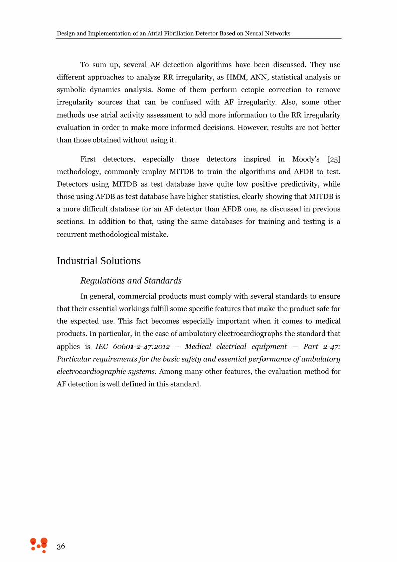
Figure 14. Graphical representation of the evaluation method attending both to episode and duration evaluation as defined in IEC 60601-2-47:2012.
The standard specifies that sensitivity and positive predictivity must be
calculated both for AF episode and its duration:
Measurement of AF episode sensitivity and positive predictivity: each
reference episode for which overlap exists is counted as a true positive
for purposes of determining AF episode sensitivity; any other reference
episodes are counted as false negatives. Similarly, each algorithm-
marked episode for which overlap exists is counted as a true positive for
purposes of determining AF episode positive predictivity; any other
algorithm-marked episodes are counted as false positives.
Measurement of AF duration sensitivity and positive predictivity
requires determination of the total duration of reference and algorithm-
marked VF and of the total duration of periods of overlap as defined
above.[39]
Figure 14 shows a graphical representation of the evaluation method attending
both to the episode and the duration statistics defined above.
The standard also specifies that MIT-BIH Arrhythmia Database must be used
for evaluating AF detection, although it is not specified if this database must be used
during to train the system or not.
Design and Implementation of an Atrial Fibrillation Detector Based on Neural Networks
38
Commercial Products
Despite AF evaluation is clearly disclosed in the standard, AF detection statistics
of a commercial product are susceptible data and so they are not clearly disclosed. For
example, AliveCor is a company that have developed an FDA-cleared mobile phone
case with built-in electrodes to record short ECGs from the fingers of the patient. Their
product is aimed to be a tool for detection and control of AF patients, in order to reduce
the associated morbidity and mortality. However, no AF detection statistics are
disclosed in their corporative web page.
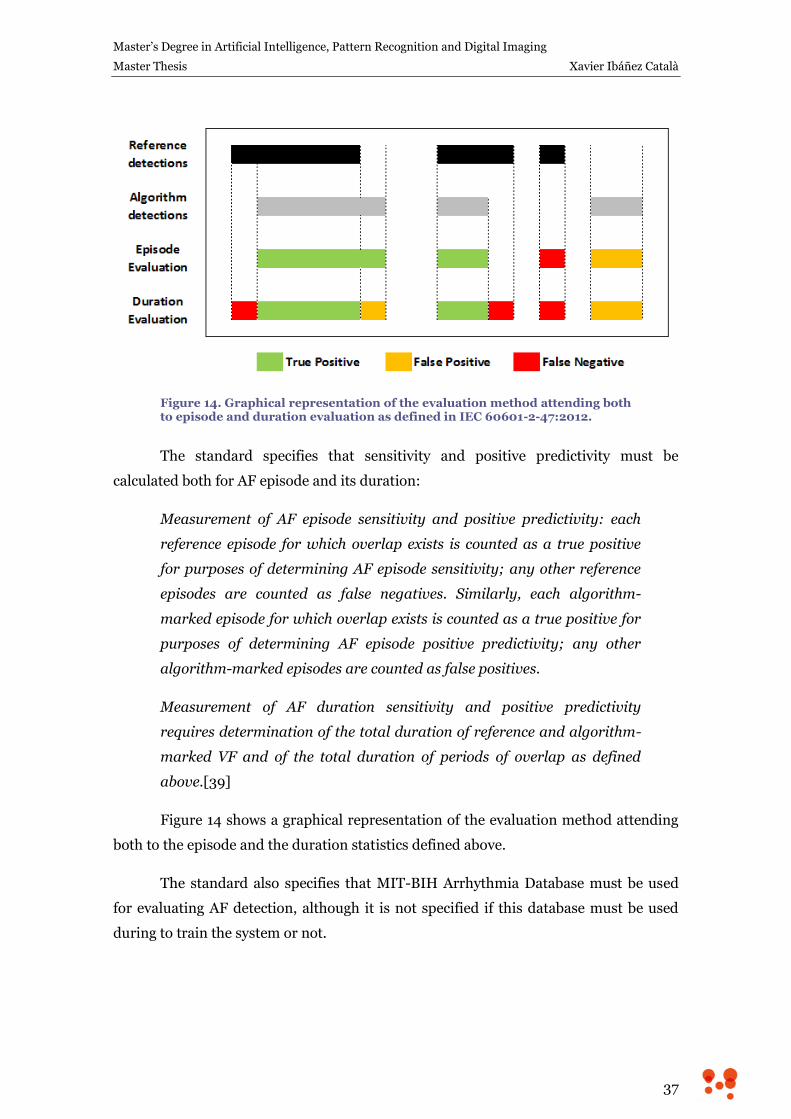
In this section, AF detection results of some commercial products are disclosed.
Table 2 shows a comparative of AF detection results of several commercial products
which results have been published. GE Marquett 12SL is a diagnosis algorithm for 12-
lead ECG developed by General Electric. Kinetic™ AF ECG Algorithm is part of a family
of algorithms to process ECG developed by Monebo Technologies, who licenses its
algorithms to third parties, as CardioComm Solutions Inc. or Freescale
Semiconductors. DLX ECG Algorithm is used by Philips in different cardiac monitoring
solutions. Reveal LINQ and SEEQ are both products from Medtronic and have been
reviewed previously.
Table 2. Comparative of AF detection results of several commercial products.
Sens (%) +P (%) Database
GE Marquett 12SL 87.5 95.4 Private: 10761 records.
Kinetic™ AF ECG Algorithm 95.7 83.3 Private: 250 records.
DLX ECG Algorithm 89.0 90.0 Private: 1785 records.
Reveal LINQ 97.4 84.4 Private: 150 records.
SEEQ (Medtronic) 90.0 85.0
MITDB, as specified in
IEC 60601-2-47
(duration assesment)
As it can be seen, all products except SEEQ use private database, so compare
results is not possible. To our concern, only SEEQ shows AF detection results on
MITDB but it is not disclosed if this database was only used for testing or was also used
for training the algorithm. However, it seems obvious that Medtronic, after doing their
best for the development of their AF detector, would had performed a last train of the
system including MITDB in the training data to obtain the best possible performance.
Master’s Degree in Artificial Intelligence, Pattern Recognition and Digital Imaging
Master Thesis Xavier Ibáñez Català
39
Moreover, they also declare that the statistics stands for the duration assessment and
the evaluation has been performed as specified in standard IEC 60601-2-47.
Performance Goals
As it was declared, the main objective of this Master Thesis is to develop a
classification system able to distinguish between AF and non-AF rhythms.
AF is clinically defined as an irregular cardiac rhythm of narrow beats
(supraventricular origin) where no P wave can be distinguished maintained during 30
seconds at least [4]. Therefore, the developed system should only use the inter-beat
intervals information contained in 30 seconds segments of ECG signal to perform the
classification. Thus, no morphology assessed rejection should be made to eliminate
ectopic beats that can be confused with AF rhythm and every beat should be considered
to generate the RR interval. This way, the classifier could be integrated in any ECG
analysis system that performs beat detection, such as implantable or external cardiac
monitors or offline analysis platforms as holter analysis software.
The performance goal of this development is to overcome the results of SEEQ,
which is, to our concern, the only commercial product shown AF detection statistics
based on IEC 60601-2-47 standard and public database. In other words, the objective is
to reach sensitivity higher than 90% and positive predictivity higher than 85% on
MITDB.
To achieve this goal, artificial neural networks will be used and several
strategies to improve the learning and generalization will be explored.

Design and Implementation of an Atrial Fibrillation Detector Based on Neural Networks
40
Master’s Degree in Artificial Intelligence, Pattern Recognition and Digital Imaging
Master Thesis Xavier Ibáñez Català
41
4. Methods
Artificial Neural Networks
Artificial Neural Networks (ANNs) are a family of statistical learning models
inspired by biological neural networks, which are formed by millions of interconnected
neurons. Natural neurons receive signals through synapses located on the dendrites or
the soma of the neuron, and, whenever the signal received is strong enough, the neuron
is activated and a signal is emitted through the axon. This signal might be sent to
another synapse and might activate other neurons of the network.
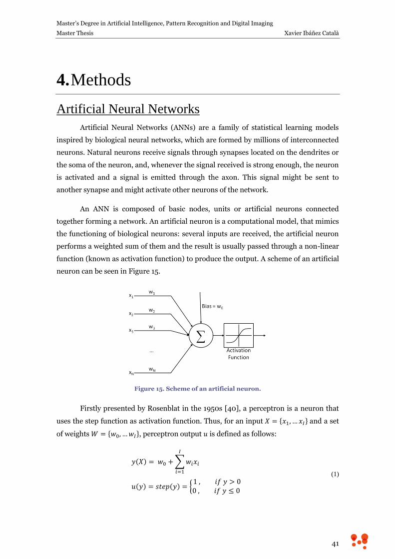
An ANN is composed of basic nodes, units or artificial neurons connected
together forming a network. An artificial neuron is a computational model, that mimics
the functioning of biological neurons: several inputs are received, the artificial neuron
performs a weighted sum of them and the result is usually passed through a non-linear
function (known as activation function) to produce the output. A scheme of an artificial
neuron can be seen in Figure 15.
Figure 15. Scheme of an artificial neuron.
Firstly presented by Rosenblat in the 1950s [40], a perceptron is a neuron that
uses the step function as activation function. Thus, for an input and a set
of weights , perceptron output is defined as follows:
(1)
Design and Implementation of an Atrial Fibrillation Detector Based on Neural Networks
42
It has been proved that a perceptron can correctly classify samples of two
classes if they are lineally separable; in other words, a perceptron is able to determine
hyperplane-shaped borders to distinguish between two classes [41]. To learn the
weights of a perceptron from classified samples, a gradient descent optimization can be
used, but the step function discontinuity and the null derivative generate numerical
problems. So continuously differentiable sigmoid-shaped functions, such as logistic
function or hyperbolic tangent, are generally used instead of the step function.
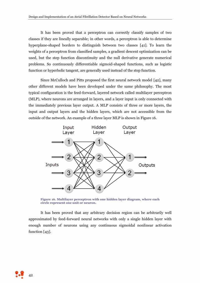
Since McCulloch and Pitts proposed the first neural network model [42], many
other different models have been developed under the same philosophy. The most
typical configuration is the feed-forward, layered network called multilayer perceptron
(MLP), where neurons are arranged in layers, and a layer input is only connected with
the immediately previous layer output. A MLP consists of three or more layers, the
input and output layers and the hidden layers, which are not accessible from the
outside of the network. An example of a three layer MLP is shown in Figure 16.
Figure 16. Multilayer perceptron with one hidden layer diagram, where each circle represent one unit or neuron.
It has been proved that any arbitrary decision region can be arbitrarily well
approximated by feed-forward neural networks with only a single hidden layer with
enough number of neurons using any continuous sigmoidal nonlinear activation
function [43].
Master’s Degree in Artificial Intelligence, Pattern Recognition and Digital Imaging
Master Thesis Xavier Ibáñez Català
43
Backpropagation
A key step in using an MLP model is to choose the optimal weights that
represent the problem. Backpropagation method, proposed by Rumelhart et al in 1986
[44], is commonly used for that task. The basic idea of this method is to backpropagate
the errors in order to modify each weight by applying gradient descent to them. In
order to calculate the error, backpropagation requires a known desired output for each
input sample, so labeled samples are needed for training.
Let say that the neural network computes a function , where refers
to the p-th input sample, and W represents the collection of adjustable parameters in
the system. An error function , measures de discrepancy between
the desired output for the sample and the output produced by the system. The
sum of the squared differences is usually employed as an error measure, but any other
function can be used. Thus, each weight (weight i of the neuron j of the layer n)
should be modified as follows:
(2)
Where is the learning rate, and E can be the error of one sample ( ), the
average error of a subset of the training dataset or the average error of the whole
training dataset. Weights can be updated using these different errors, leading to
stochastic, mini-batch or batch learning, respectively.
Once error is computed, can be calculated by using the chain rule for
partial derivation. For example, if a simplified case of one output neuron is considered,
error only depends on scalars , the desired output, and , the output of the
system. can be written as a function of the last neuron inputs using
equation (1).
(3)
Where refers to the output of the previous layer, which is the input of layer
N as well. Thus, the partial derivative of the error with respect to is:
(4)
Design and Implementation of an Atrial Fibrillation Detector Based on Neural Networks
44
This procedure can be continued to determine the update term of any other
weight of any other layer just by backpropagating the partial derivative of the error.
The election of the activation function is of great importance to optimize the
learning process. For example, using logistic or hyperbolic tangent is very efficient
because their derivatives are defined in terms of the non differentiated function, and
this value was calculated while evaluating the sample, so no computation is needed to
calculate the derivative of the activation function:
Logistic function:
(5)
Hyperbolic Tangent:
(6)
Output Units for Classification
When an ANN is used as a classifier, output neurons generally implement
softmax activation function instead of sigmoid. The main advantage of using softmax is
that it produces an output that can be interpreted as posteriori probability of belonging
to a particular class.
Softmax function is a transformation that normalizes a K-dimensional vector
of arbitrary real values to a K-dimensional vector of real values in the range [0, 1].
It is defined as follows:
(7)
If squared difference is taken as an error function, it is easy to see that gradient
of the error is complicated and propagated errors will depend on the activations of all
neighbor neurons, which is quite inconvenient for the computational performance of
the learning process. However, if cross-entropy is used as an error function, it can be
demonstrated that the gradient of the error turns into a linear function of the desired
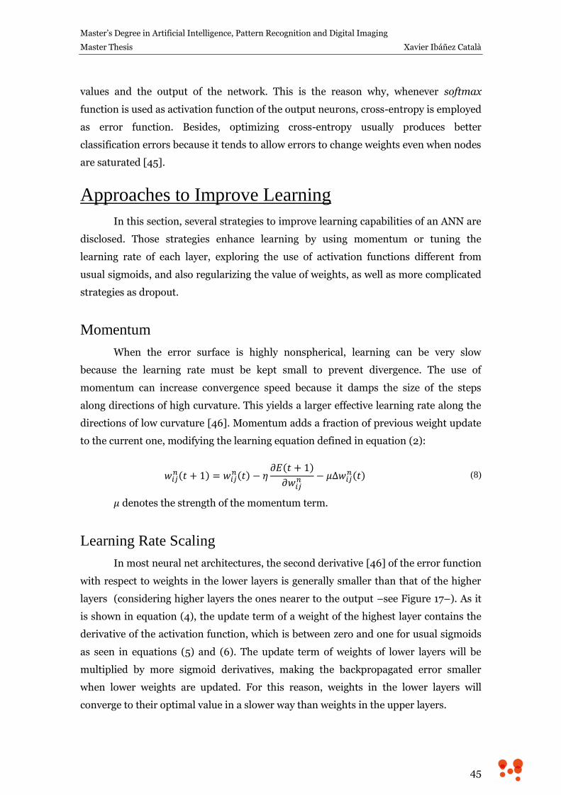
Master’s Degree in Artificial Intelligence, Pattern Recognition and Digital Imaging
Master Thesis Xavier Ibáñez Català
45
values and the output of the network. This is the reason why, whenever softmax
function is used as activation function of the output neurons, cross-entropy is employed
as error function. Besides, optimizing cross-entropy usually produces better
classification errors because it tends to allow errors to change weights even when nodes
are saturated [45].
Approaches to Improve Learning
In this section, several strategies to improve learning capabilities of an ANN are
disclosed. Those strategies enhance learning by using momentum or tuning the
learning rate of each layer, exploring the use of activation functions different from
usual sigmoids, and also regularizing the value of weights, as well as more complicated
strategies as dropout.
Momentum
When the error surface is highly nonspherical, learning can be very slow
because the learning rate must be kept small to prevent divergence. The use of
momentum can increase convergence speed because it damps the size of the steps
along directions of high curvature. This yields a larger effective learning rate along the
directions of low curvature [46]. Momentum adds a fraction of previous weight update
to the current one, modifying the learning equation defined in equation (2):
(8)
denotes the strength of the momentum term.
Learning Rate Scaling
In most neural net architectures, the second derivative [46] of the error function
with respect to weights in the lower layers is generally smaller than that of the higher
layers (considering higher layers the ones nearer to the output –see Figure 17–). As it
is shown in equation (4), the update term of a weight of the highest layer contains the
derivative of the activation function, which is between zero and one for usual sigmoids
as seen in equations (5) and (6). The update term of weights of lower layers will be
multiplied by more sigmoid derivatives, making the backpropagated error smaller
when lower weights are updated. For this reason, weights in the lower layers will
converge to their optimal value in a slower way than weights in the upper layers.
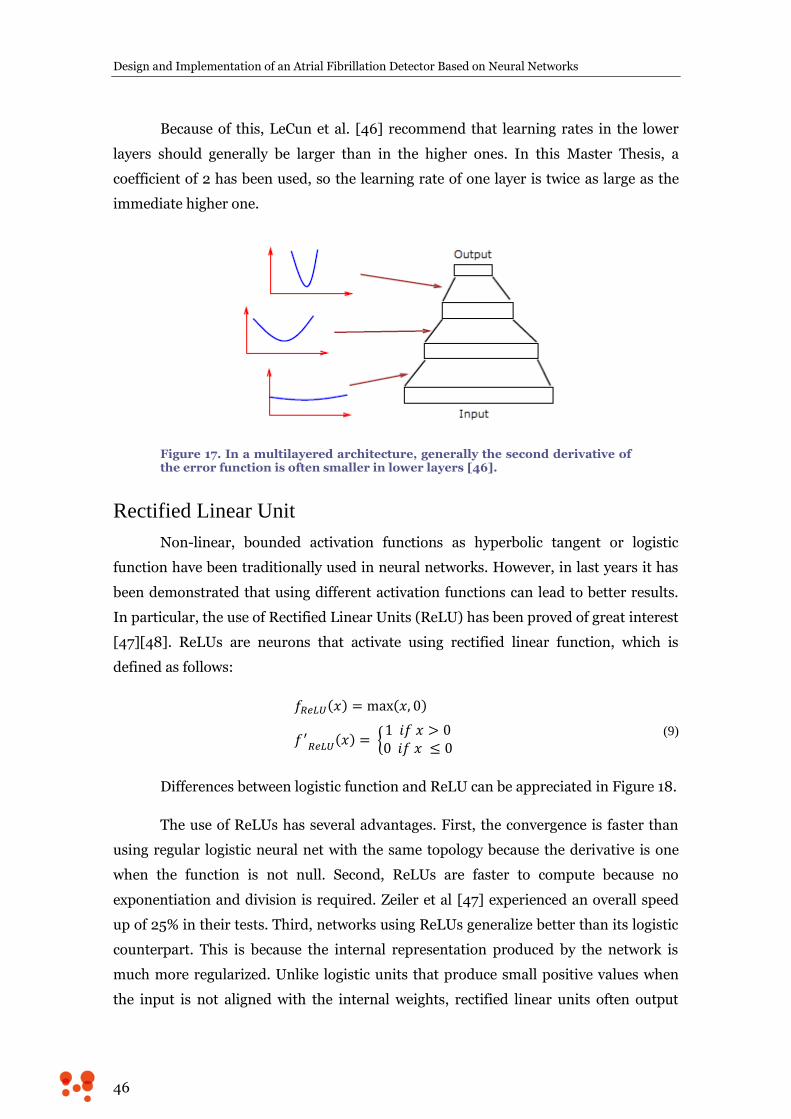
Design and Implementation of an Atrial Fibrillation Detector Based on Neural Networks
46
Because of this, LeCun et al. [46] recommend that learning rates in the lower
layers should generally be larger than in the higher ones. In this Master Thesis, a
coefficient of 2 has been used, so the learning rate of one layer is twice as large as the
immediate higher one.
Figure 17. In a multilayered architecture, generally the second derivative of the error function is often smaller in lower layers [46].
Rectified Linear Unit
Non-linear, bounded activation functions as hyperbolic tangent or logistic
function have been traditionally used in neural networks. However, in last years it has
been demonstrated that using different activation functions can lead to better results.
In particular, the use of Rectified Linear Units (ReLU) has been proved of great interest
[47][48]. ReLUs are neurons that activate using rectified linear function, which is
defined as follows:
(9)
Differences between logistic function and ReLU can be appreciated in Figure 18.
The use of ReLUs has several advantages. First, the convergence is faster than
using regular logistic neural net with the same topology because the derivative is one
when the function is not null. Second, ReLUs are faster to compute because no
exponentiation and division is required. Zeiler et al [47] experienced an overall speed
up of 25% in their tests. Third, networks using ReLUs generalize better than its logistic
counterpart. This is because the internal representation produced by the network is
much more regularized. Unlike logistic units that produce small positive values when
the input is not aligned with the internal weights, rectified linear units often output
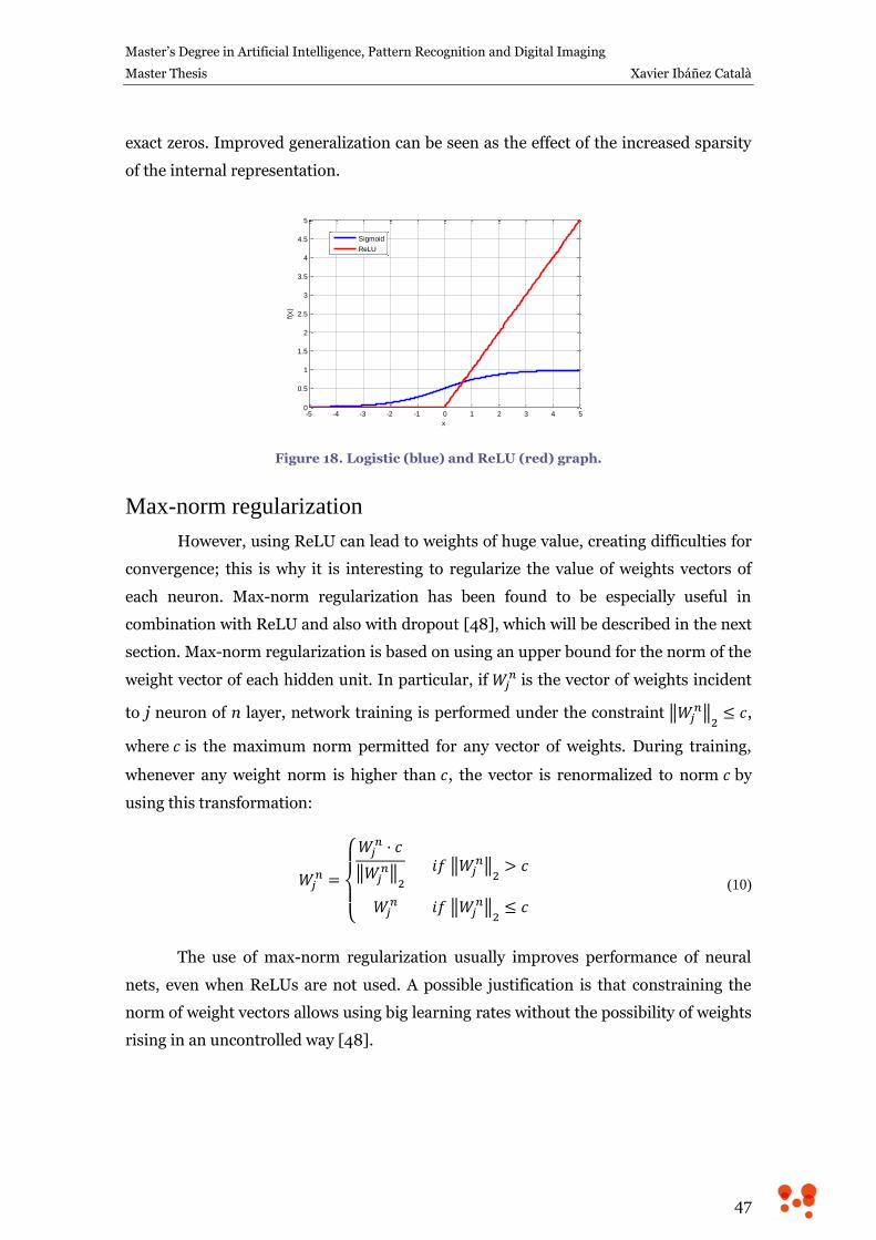
Master’s Degree in Artificial Intelligence, Pattern Recognition and Digital Imaging
Master Thesis Xavier Ibáñez Català
47
exact zeros. Improved generalization can be seen as the effect of the increased sparsity
of the internal representation.
Figure 18. Logistic (blue) and ReLU (red) graph.
Max-norm regularization
However, using ReLU can lead to weights of huge value, creating difficulties for
convergence; this is why it is interesting to regularize the value of weights vectors of
each neuron. Max-norm regularization has been found to be especially useful in
combination with ReLU and also with dropout [48], which will be described in the next
section. Max-norm regularization is based on using an upper bound for the norm of the
weight vector of each hidden unit. In particular, if is the vector of weights incident
to j neuron of n layer, network training is performed under the constraint
,
where is the maximum norm permitted for any vector of weights. During training,
whenever any weight norm is higher than , the vector is renormalized to norm by
using this transformation:
(10)
The use of max-norm regularization usually improves performance of neural
nets, even when ReLUs are not used. A possible justification is that constraining the
norm of weight vectors allows using big learning rates without the possibility of weights
rising in an uncontrolled way [48].
-5 -4 -3 -2 -1 0 1 2 3 4 50
0.5
1
1.5
2
2.5
3
3.5
4
4.5
5
x
f(x)
Sigmoid
ReLU
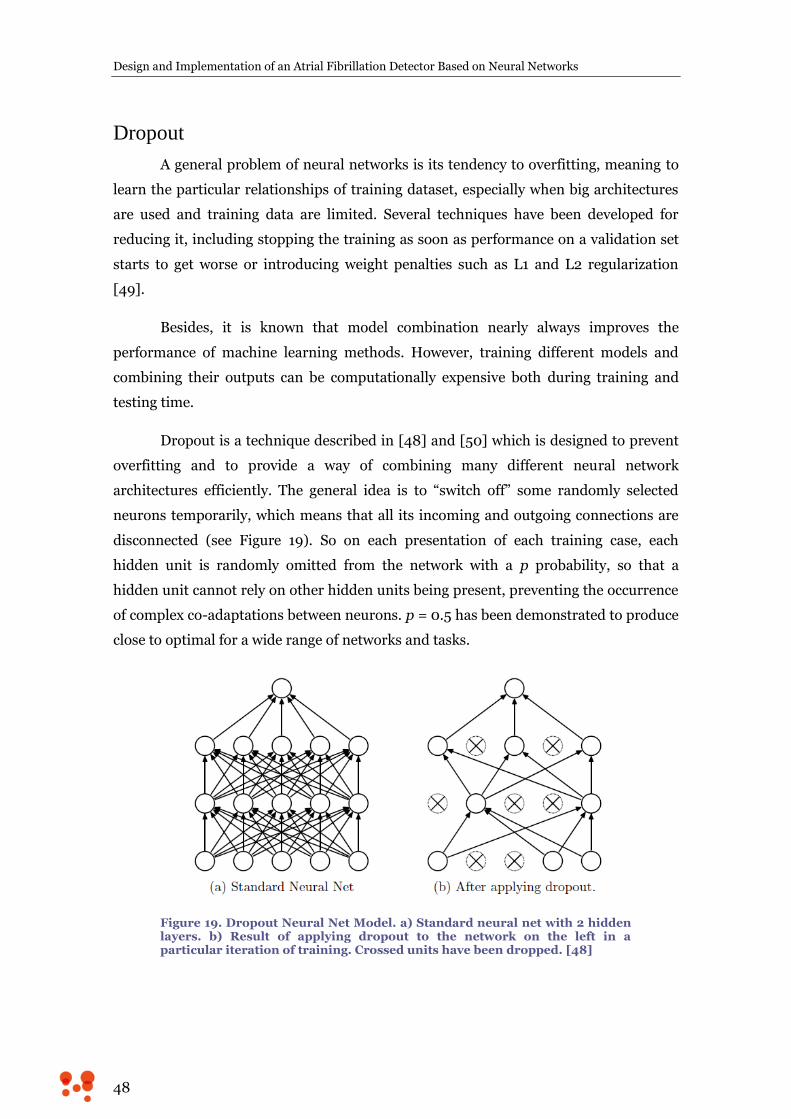
Design and Implementation of an Atrial Fibrillation Detector Based on Neural Networks
48
Dropout
A general problem of neural networks is its tendency to overfitting, meaning to
learn the particular relationships of training dataset, especially when big architectures
are used and training data are limited. Several techniques have been developed for
reducing it, including stopping the training as soon as performance on a validation set
starts to get worse or introducing weight penalties such as L1 and L2 regularization
[49].
Besides, it is known that model combination nearly always improves the
performance of machine learning methods. However, training different models and
combining their outputs can be computationally expensive both during training and
testing time.
Dropout is a technique described in [48] and [50] which is designed to prevent
overfitting and to provide a way of combining many different neural network
architectures efficiently. The general idea is to “switch off” some randomly selected
neurons temporarily, which means that all its incoming and outgoing connections are
disconnected (see Figure 19). So on each presentation of each training case, each
hidden unit is randomly omitted from the network with a p probability, so that a
hidden unit cannot rely on other hidden units being present, preventing the occurrence
of complex co-adaptations between neurons. p = 0.5 has been demonstrated to produce
close to optimal for a wide range of networks and tasks.
Figure 19. Dropout Neural Net Model. a) Standard neural net with 2 hidden layers. b) Result of applying dropout to the network on the left in a particular iteration of training. Crossed units have been dropped. [48]
Master’s Degree in Artificial Intelligence, Pattern Recognition and Digital Imaging
Master Thesis Xavier Ibáñez Català
49
That way, training a neural net with n units with dropout can be seen as training
a collection of 2n possible networks with a tiny fraction of the training data where all
networks share weights. During test time, an “averaged network” that contains all
hidden units activated is employed, but then their outgoing weights must be halved to
compensate the fact that all of them are active and not only half of them as during
training. This is approximately equivalent to calculate the geometric mean of the
probability distributions over labels predicted by all 2n possible networks.
Dropout introduces a significant amount of noise in the gradients compared to
standard stochastic gradient descent. A recommended way to reduce the effect of noise
is to use a high momentum, between 0.95 and 0.99 [48]. Momentum of 0.95 has been
used in this essay when using dropout.
Toolbox
Deep Learn Toolbox for Matlab, developed by Rasmus Berg Palm for his Master
Thesis [51], was used for training and testing the different architectures and techniques
explored in this Master Thesis. The toolbox includes logistic and softmax activation,
and also options to control dropout fraction and momentum. Learning rate scaling,
ReLU activation function and max-norm regularization were implemented to expand
the functionality of the toolbox.

Design and Implementation of an Atrial Fibrillation Detector Based on Neural Networks
50
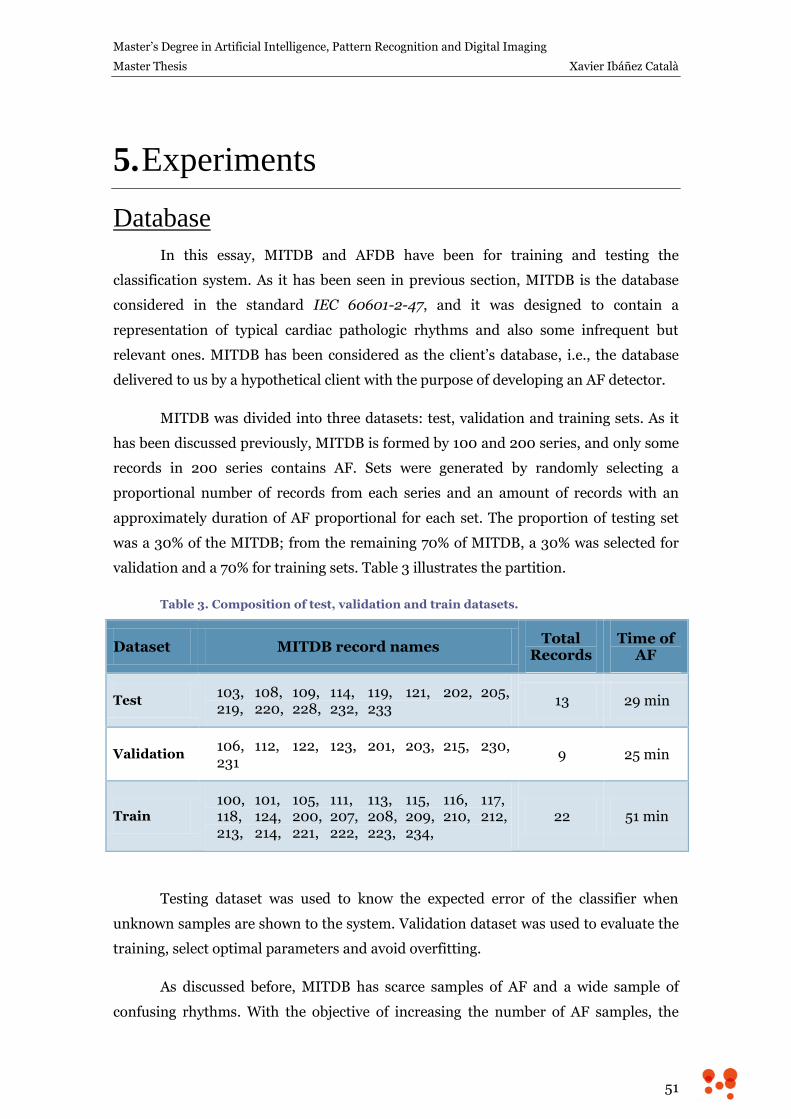
Master’s Degree in Artificial Intelligence, Pattern Recognition and Digital Imaging
Master Thesis Xavier Ibáñez Català
51
5. Experiments
Database
In this essay, MITDB and AFDB have been for training and testing the
classification system. As it has been seen in previous section, MITDB is the database
considered in the standard IEC 60601-2-47, and it was designed to contain a
representation of typical cardiac pathologic rhythms and also some infrequent but
relevant ones. MITDB has been considered as the client’s database, i.e., the database
delivered to us by a hypothetical client with the purpose of developing an AF detector.
MITDB was divided into three datasets: test, validation and training sets. As it
has been discussed previously, MITDB is formed by 100 and 200 series, and only some
records in 200 series contains AF. Sets were generated by randomly selecting a
proportional number of records from each series and an amount of records with an
approximately duration of AF proportional for each set. The proportion of testing set
was a 30% of the MITDB; from the remaining 70% of MITDB, a 30% was selected for
validation and a 70% for training sets. Table 3 illustrates the partition.
Table 3. Composition of test, validation and train datasets.
Dataset MITDB record names Total
Records Time of
AF
Test 103, 108, 109, 114, 119, 121, 202, 205,
219, 220, 228, 232, 233 13 29 min
Validation 106, 112, 122, 123, 201, 203, 215, 230,
231 9 25 min
Train 100, 101, 105, 111, 113, 115, 116, 117,
118, 124, 200, 207, 208, 209, 210, 212, 213, 214, 221, 222, 223, 234,
22 51 min
Testing dataset was used to know the expected error of the classifier when
unknown samples are shown to the system. Validation dataset was used to evaluate the
training, select optimal parameters and avoid overfitting.
As discussed before, MITDB has scarce samples of AF and a wide sample of
confusing rhythms. With the objective of increasing the number of AF samples, the
Design and Implementation of an Atrial Fibrillation Detector Based on Neural Networks
52
training dataset was enriched by adding the whole AFDB. The benefits of including
AFDB in the training dataset are evaluated in next sections.
As it was disclosed in the development goals, the system should classify
segments of 30 seconds of ECG. Thus, each signal was divided into 30-second segments
of AF or non-AF rhythm. Segments containing a part of AF and a part of non-AF
rhythm were discarded with the aim of letting the classifier to resolve the mixed cases.
Feature Extraction
As it was discussed in chapter 2, several ways of assess RR irregularity have
been used in the specific literature. Among all of them, the study of the differences
between consecutive RR intervals is a computationally simple and descriptive measure
of the irregularity, defined as . In addition to that, the use of RR
differences has the advantage of being invariant to heart rate.
Here, Lorentz plot, which is a scatter plot of vs. , have been used to
describe the irregularity of RR interval. Each point of a Lorentz plot encodes the
uncorrelated nature of three consecutive RR intervals. For example, if three consecutive
RR intervals are very similar, the corresponding Lorentz point will be near (0, 0) point.
For a short-medium-long sequence, the Lorentz point will be in the first quadrant;
long-short-long, in the second quadrant; long-medium-short, in the third quadrant;
short-long-short, in the fourth quadrant.
It has been proven that several arrhythmias imprint specific signatures on two
dimensional Lorentz plots [52], although the mixture of arrhythmias or some complex
ventricular rhythms can generate confusing patterns. In Figure 20 the Lorentz
signature of some rhythms is shown.
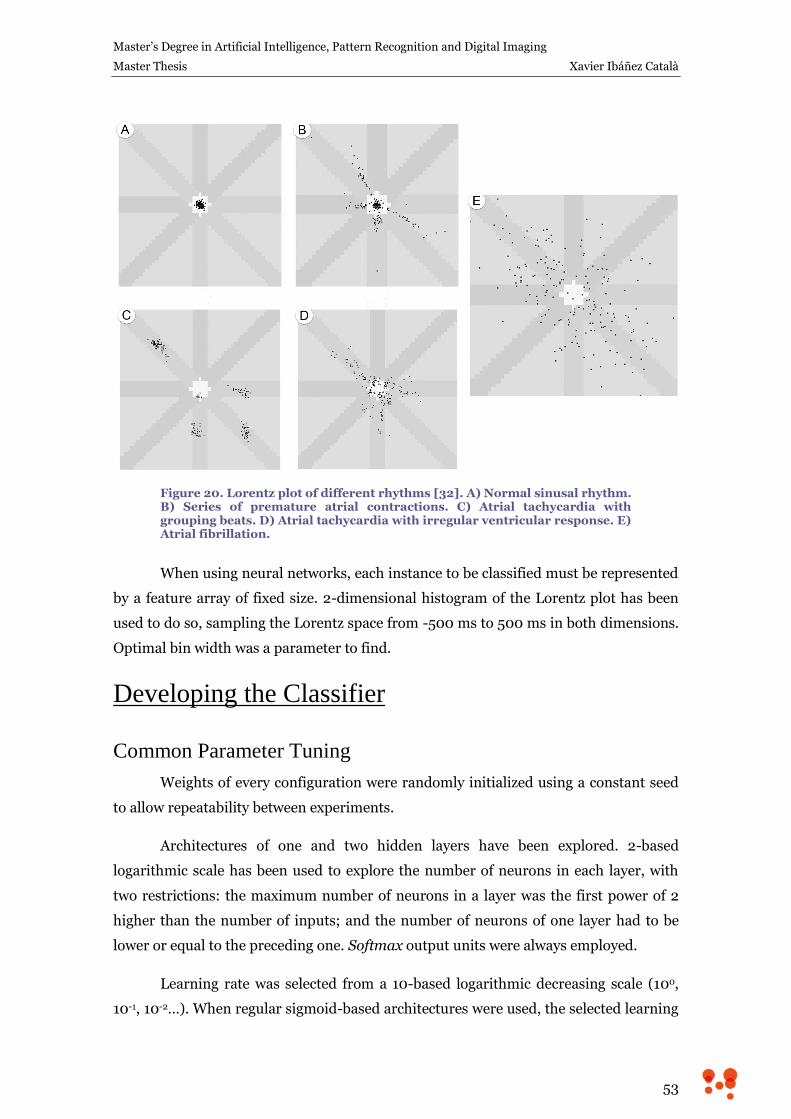
Master’s Degree in Artificial Intelligence, Pattern Recognition and Digital Imaging
Master Thesis Xavier Ibáñez Català
53
Figure 20. Lorentz plot of different rhythms [32]. A) Normal sinusal rhythm. B) Series of premature atrial contractions. C) Atrial tachycardia with grouping beats. D) Atrial tachycardia with irregular ventricular response. E) Atrial fibrillation.
When using neural networks, each instance to be classified must be represented
by a feature array of fixed size. 2-dimensional histogram of the Lorentz plot has been
used to do so, sampling the Lorentz space from -500 ms to 500 ms in both dimensions.
Optimal bin width was a parameter to find.
Developing the Classifier
Common Parameter Tuning
Weights of every configuration were randomly initialized using a constant seed
to allow repeatability between experiments.
Architectures of one and two hidden layers have been explored. 2-based
logarithmic scale has been used to explore the number of neurons in each layer, with
two restrictions: the maximum number of neurons in a layer was the first power of 2
higher than the number of inputs; and the number of neurons of one layer had to be
lower or equal to the preceding one. Softmax output units were always employed.
Learning rate was selected from a 10-based logarithmic decreasing scale (100,
10-1, 10-2…). When regular sigmoid-based architectures were used, the selected learning
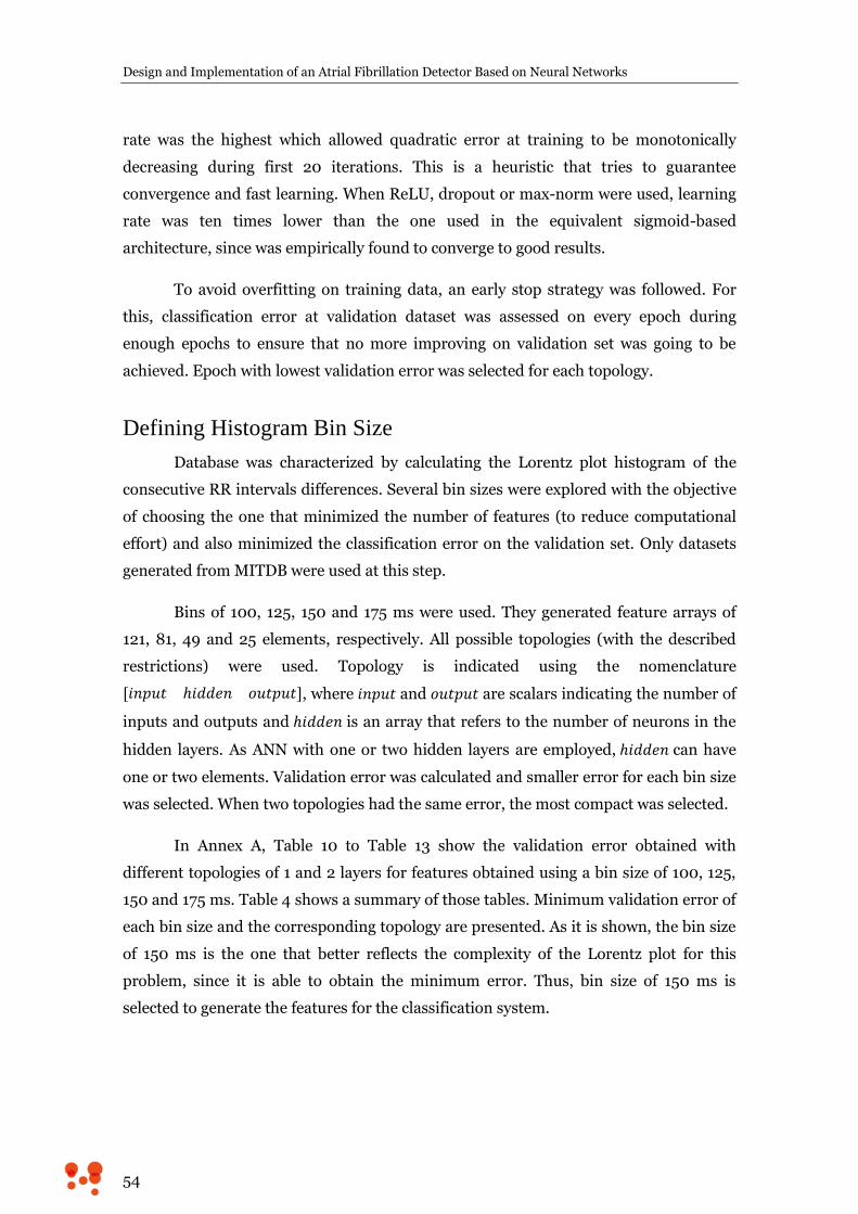
Design and Implementation of an Atrial Fibrillation Detector Based on Neural Networks
54
rate was the highest which allowed quadratic error at training to be monotonically
decreasing during first 20 iterations. This is a heuristic that tries to guarantee
convergence and fast learning. When ReLU, dropout or max-norm were used, learning
rate was ten times lower than the one used in the equivalent sigmoid-based
architecture, since was empirically found to converge to good results.
To avoid overfitting on training data, an early stop strategy was followed. For
this, classification error at validation dataset was assessed on every epoch during
enough epochs to ensure that no more improving on validation set was going to be
achieved. Epoch with lowest validation error was selected for each topology.
Defining Histogram Bin Size
Database was characterized by calculating the Lorentz plot histogram of the
consecutive RR intervals differences. Several bin sizes were explored with the objective
of choosing the one that minimized the number of features (to reduce computational
effort) and also minimized the classification error on the validation set. Only datasets
generated from MITDB were used at this step.
Bins of 100, 125, 150 and 175 ms were used. They generated feature arrays of
121, 81, 49 and 25 elements, respectively. All possible topologies (with the described
restrictions) were used. Topology is indicated using the nomenclature
, where and are scalars indicating the number of
inputs and outputs and is an array that refers to the number of neurons in the
hidden layers. As ANN with one or two hidden layers are employed, can have
one or two elements. Validation error was calculated and smaller error for each bin size
was selected. When two topologies had the same error, the most compact was selected.
In Annex A, Table 10 to Table 13 show the validation error obtained with
different topologies of 1 and 2 layers for features obtained using a bin size of 100, 125,
150 and 175 ms. Table 4 shows a summary of those tables. Minimum validation error of
each bin size and the corresponding topology are presented. As it is shown, the bin size
of 150 ms is the one that better reflects the complexity of the Lorentz plot for this
problem, since it is able to obtain the minimum error. Thus, bin size of 150 ms is
selected to generate the features for the classification system.
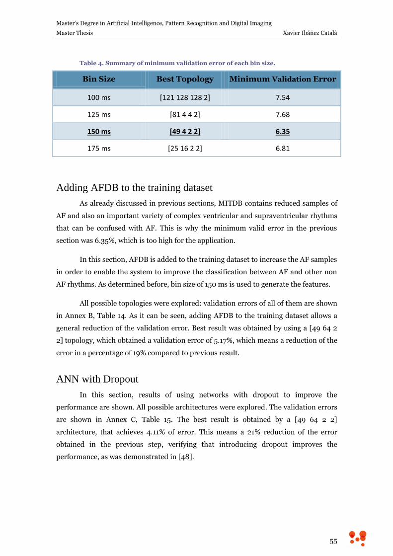
Master’s Degree in Artificial Intelligence, Pattern Recognition and Digital Imaging
Master Thesis Xavier Ibáñez Català
55
Table 4. Summary of minimum validation error of each bin size.
Bin Size Best Topology Minimum Validation Error
100 ms [121 128 128 2] 7.54
125 ms [81 4 4 2] 7.68
150 ms [49 4 2 2] 6.35
175 ms [25 16 2 2] 6.81
Adding AFDB to the training dataset
As already discussed in previous sections, MITDB contains reduced samples of
AF and also an important variety of complex ventricular and supraventricular rhythms
that can be confused with AF. This is why the minimum valid error in the previous
section was 6.35%, which is too high for the application.
In this section, AFDB is added to the training dataset to increase the AF samples
in order to enable the system to improve the classification between AF and other non
AF rhythms. As determined before, bin size of 150 ms is used to generate the features.
All possible topologies were explored: validation errors of all of them are shown
in Annex B, Table 14. As it can be seen, adding AFDB to the training dataset allows a
general reduction of the validation error. Best result was obtained by using a [49 64 2
2] topology, which obtained a validation error of 5.17%, which means a reduction of the
error in a percentage of 19% compared to previous result.
ANN with Dropout
In this section, results of using networks with dropout to improve the
performance are shown. All possible architectures were explored. The validation errors
are shown in Annex C, Table 15. The best result is obtained by a [49 64 2 2]
architecture, that achieves 4.11% of error. This means a 21% reduction of the error
obtained in the previous step, verifying that introducing dropout improves the
performance, as was demonstrated in [48].
Design and Implementation of an Atrial Fibrillation Detector Based on Neural Networks
56
ANN with Dropout and ReLU
Using the best architecture of the previous section, the network was modified to
use ReLU in hidden layers and training was performed again. No regularization was
introduced in this step. This configuration obtained a validation error of 4.75%, which
was worse than the one without ReLU. This is because ReLU propagates big gradients
and weights can reach huge values in an uncontrolled way, converging to a sub-optimal
solution. In this case, max-norm regularization should be used.
Apply max-norm regularization
In order to control the norm of weight vectors of the ReLU configurations, max-
norm regularization was used. 2, 3 and 4 were used as max-norm coefficients, and
validation error was calculated this way. Results are shown in Table 5.
Table 5. Validation error of networks using dropout and ReLU and different max-norm coefficients.
Max-norm coefficient
Topology Validation Error (%)
2 [49 64 2 2] 4.65
3 [49 64 2 2] 3.47
4 [49 64 2 2] 3.45
As it can be seen, the best validation error is obtained using a max-norm
regularization coefficient of 4. This configuration achieves a validation error of 3.45%,
which means a 16% reduction of the error obtained using only dropout, and also a 27%
reduction of the error obtained using dropout and ReLU without regularization.
Conclusion
Several strategies have been implemented to improve the performance of a
classifier based on ANN. First strategy was to enrich the training dataset with more
samples to represent the classes in a better way, obtaining a reduction of 19% in the.
validation error Secondly, dropout was used, and error was reduced a 21% more. Third,
ReLU was used and, if no regularization was used, the error became worse. However, if
max-norm regularization with a coefficient of 4 was used, the error was reduced again
by 16%. Results are shown in Table 6. Summing up, from the first to the last step, the
error was reduced by a 45%.
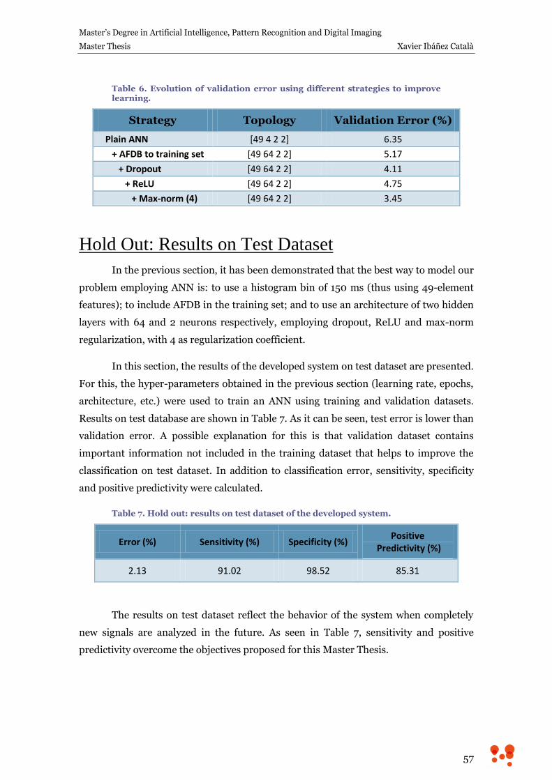
Master’s Degree in Artificial Intelligence, Pattern Recognition and Digital Imaging
Master Thesis Xavier Ibáñez Català
57
Table 6. Evolution of validation error using different strategies to improve learning.
Strategy Topology Validation Error (%)
Plain ANN [49 4 2 2] 6.35
+ AFDB to training set [49 64 2 2] 5.17
+ Dropout [49 64 2 2] 4.11
+ ReLU [49 64 2 2] 4.75
+ Max-norm (4) [49 64 2 2] 3.45
Hold Out: Results on Test Dataset
In the previous section, it has been demonstrated that the best way to model our
problem employing ANN is: to use a histogram bin of 150 ms (thus using 49-element
features); to include AFDB in the training set; and to use an architecture of two hidden
layers with 64 and 2 neurons respectively, employing dropout, ReLU and max-norm
regularization, with 4 as regularization coefficient.
In this section, the results of the developed system on test dataset are presented.
For this, the hyper-parameters obtained in the previous section (learning rate, epochs,
architecture, etc.) were used to train an ANN using training and validation datasets.
Results on test database are shown in Table 7. As it can be seen, test error is lower than
validation error. A possible explanation for this is that validation dataset contains
important information not included in the training dataset that helps to improve the
classification on test dataset. In addition to classification error, sensitivity, specificity
and positive predictivity were calculated.
Table 7. Hold out: results on test dataset of the developed system.
Error (%) Sensitivity (%) Specificity (%) Positive
Predictivity (%)
2.13 91.02 98.52 85.31
The results on test dataset reflect the behavior of the system when completely
new signals are analyzed in the future. As seen in Table 7, sensitivity and positive
predictivity overcome the objectives proposed for this Master Thesis.

Design and Implementation of an Atrial Fibrillation Detector Based on Neural Networks
58
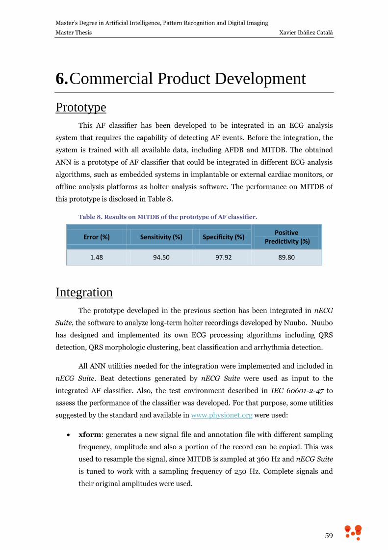
Master’s Degree in Artificial Intelligence, Pattern Recognition and Digital Imaging
Master Thesis Xavier Ibáñez Català
59
6. Commercial Product Development
Prototype
This AF classifier has been developed to be integrated in an ECG analysis
system that requires the capability of detecting AF events. Before the integration, the
system is trained with all available data, including AFDB and MITDB. The obtained
ANN is a prototype of AF classifier that could be integrated in different ECG analysis
algorithms, such as embedded systems in implantable or external cardiac monitors, or
offline analysis platforms as holter analysis software. The performance on MITDB of
this prototype is disclosed in Table 8.
Table 8. Results on MITDB of the prototype of AF classifier.
Error (%) Sensitivity (%) Specificity (%) Positive
Predictivity (%)
1.48 94.50 97.92 89.80
Integration
The prototype developed in the previous section has been integrated in nECG
Suite, the software to analyze long-term holter recordings developed by Nuubo. Nuubo
has designed and implemented its own ECG processing algorithms including QRS
detection, QRS morphologic clustering, beat classification and arrhythmia detection.
All ANN utilities needed for the integration were implemented and included in
nECG Suite. Beat detections generated by nECG Suite were used as input to the
integrated AF classifier. Also, the test environment described in IEC 60601-2-47 to
assess the performance of the classifier was developed. For that purpose, some utilities
suggested by the standard and available in www.physionet.org were used:
xform: generates a new signal file and annotation file with different sampling
frequency, amplitude and also a portion of the record can be copied. This was
used to resample the signal, since MITDB is sampled at 360 Hz and nECG Suite
is tuned to work with a sampling frequency of 250 Hz. Complete signals and
their original amplitudes were used.
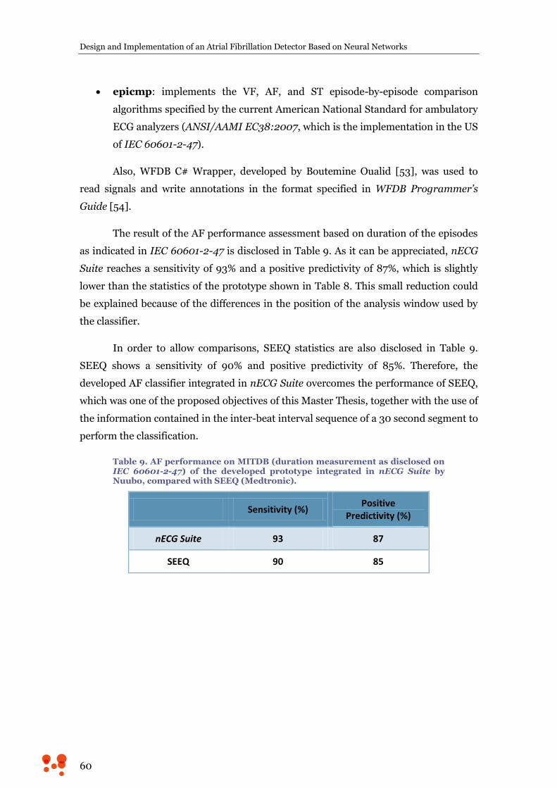
Design and Implementation of an Atrial Fibrillation Detector Based on Neural Networks
60
epicmp: implements the VF, AF, and ST episode-by-episode comparison
algorithms specified by the current American National Standard for ambulatory
ECG analyzers (ANSI/AAMI EC38:2007, which is the implementation in the US
of IEC 60601-2-47).
Also, WFDB C# Wrapper, developed by Boutemine Oualid [53], was used to
read signals and write annotations in the format specified in WFDB Programmer’s
Guide [54].
The result of the AF performance assessment based on duration of the episodes
as indicated in IEC 60601-2-47 is disclosed in Table 9. As it can be appreciated, nECG
Suite reaches a sensitivity of 93% and a positive predictivity of 87%, which is slightly
lower than the statistics of the prototype shown in Table 8. This small reduction could
be explained because of the differences in the position of the analysis window used by
the classifier.
In order to allow comparisons, SEEQ statistics are also disclosed in Table 9.
SEEQ shows a sensitivity of 90% and positive predictivity of 85%. Therefore, the
developed AF classifier integrated in nECG Suite overcomes the performance of SEEQ,
which was one of the proposed objectives of this Master Thesis, together with the use of
the information contained in the inter-beat interval sequence of a 30 second segment to
perform the classification.
Table 9. AF performance on MITDB (duration measurement as disclosed on IEC 60601-2-47) of the developed prototype integrated in nECG Suite by Nuubo, compared with SEEQ (Medtronic).
Sensitivity (%) Positive
Predictivity (%)
nECG Suite 93 87
SEEQ 90 85
Master’s Degree in Artificial Intelligence, Pattern Recognition and Digital Imaging
Master Thesis Xavier Ibáñez Català
61
7. Conclusions
The main goal of this Master Thesis was to develop a classifier able to
distinguish between atrial fibrillation (AF) and non-AF rhythms using the information
contained in the inter-beat interval sequence of a segment of 30 seconds. Thus, every
detected beat is considered and no morphology assessment is needed in order to
eliminate ectopic beats that can be confused with AF rhythm. This way, the classifier
could be integrated in any ECG analysis system that performs beat detection, such as
implantable or external cardiac monitors or offline analysis platforms as holter analysis
software.
In the first section, heart physiology and AF mechanisms and symptoms have
been discussed. AF is the most common sustained arrhythmia, affecting 1–2% of the
population. It is a fast arrhythmia characterized by the set up of recurrent, multiple and
uncoordinated electrical waves in the atrium that excite the atrial myocardium in a
totally disorganized way. As a result, atrial contraction is inexistent and ventricular
beats are fast and arrhythmic. AF is associated with a 5-fold risk of stroke and an
augmented morbi-mortality of patients with AF. Also, those patients suffer from
palpitations, fatigue, faintness or shortness of breath, among other symptoms, which
considerably reduce their quality of life and their exercise capacity.
In the second section, several strategies to monitor the ECG ambulatorily were
analyzed, going from the traditional holter test to more innovative techniques focused
on long-term monitoring, as adhesive patches, textile holter or implantable cardiac
monitors. Together with this, a review of the state of the art in AF detection was
performed, considering both academic solutions and industrial solutions. Among the
industrial solutions, SEEQ (by Medtronic) is, to our concern, the only one which
publishes its AF detection statistics on public standard databases (MIT-BIH
Arrhythmia Database), achieving a sensitivity of 90% and a positive predictivity of 85%.
To overcome these statistics was an objective of this Master Thesis.
Artificial neural networks (ANN) were the chosen tool to achieve the proposed
objective. In the fourth section a brief description of ANN has been performed. And
also, several techniques to improve their learning capabilities have been discussed,
such as employing rectified linear units (ReLU) in the hidden layers or dropout
Design and Implementation of an Atrial Fibrillation Detector Based on Neural Networks
62
mechanism, which temporally disables random neurons during training time to
improve generalization.
Using public annotated database from Physionet (MIT-BIH Arrhythmia
Database and MIT-BIH Atrial Fibrillation Database), and following a hold out strategy,
three dataset were made, one to train, another to validate the results of the training and
a third one to test the final performance. Besides, best features to describe the problem
were determined by using plain ANN. Then, the mentioned techniques to improve
learning capabilities were explored in an incremental approach, verifying that each new
technique reduced the classification error on the validation dataset.
The result of this optimization process was a reduction of classification error in
a 45%. The best network had two hidden layers of 64 and 2 neurons respectively and
implemented dropout, softmax output units, ReLU in hidden layers and max-norm
regularization. On test dataset, classification error was 2.13%, sensitivity 91.02%,
specificity 98.52% and positive predictivity 85.31%. So the behavior of this classifier
when completely new signals are analyzed overcomes the proposed objective.
This classification system was prototyped to be introduced in an ECG analysis
system that requires the capability of detecting AF events. To do this, a system with the
hyper-parameters obtained in the develop stage was trained using all available data,
i.e., training, validation and test datasets. This prototype had a classification error on
MIT-BIH Arrhythmia Database of 1.48%, a sensitivity of 94.50%, a specificity of
97.92% and a positive predictivity of 89.80%.
Finally, the prototype was integrated in a software solution to analyze long-term
holter recordings developed by Nuubo, called nECG Suite. This software uses
proprietary algorithms to perform QRS detection, QRS morphology clustering, beat
classification and arrhythmia detection. Also, the test environment described in IEC
60601-2-47 to assess the performance of the classifier was developed. The evaluation
shows that nECG Suite has a sensitivity of 93% and a positive predictivity of 87%,
overcoming the proposed objective of 90% and 85% respectively fulfilling the
requirement of only using the inter-beat interval sequence contained in 30-second
segments.
Master’s Degree in Artificial Intelligence, Pattern Recognition and Digital Imaging
Master Thesis Xavier Ibáñez Català
63
8. References
[1] Guyton AC, Hall JE. Textbook of Medical Physiology, 11 ed Elsevier Saunders, 2006.
[2] Berret K, Brooks H, Boitano S, Barman S. Ganong’s Review of Medical Physiology, 23
ed. Mc Graw Hill Medical, 2010.
[3] Runge MS, Stouffer G, Patterson C. Netter’s Cardiology. Elsevier Health Sciences.
2010
[4] Camm AJ, Kirchhof P, Lip GY, et al. Guidelines for the management of atrial
fibrillation. European heart journal, 2010, v.31, pp.2369–2429.
[5] January CT, Wann LS, Alpert JS, et al. AHA/ACC/HRS guideline for the management
of patients with atrial fibrillation: a report of the American College of
Cardiology/American Heart Association Task Force on Practice Guidelines and the
Heart Rhythm Society. Journal of the American College of Cardiology, 2014, v.64(21),
pp.2246–2280.
[6] Charitos EI, Stierle U, Ziegler PD, et al. A Comprehensive Evaluation of Rhythm
Monitoring Strategies for the Detection of Atrial Fibrillation Recurrence Insights From
647 Continuously Monitored Patients and Implications for Monitoring After
Therapeutic Interventions. Circulation, 2012, v.126(7), pp.806–814.
[7] Kirchhof P, Auricchio A, Bax J, et al. Outcome parameters for trials in atrial
fibrillation: executive summary. Recommendations from a consensus conference
organized by the German Atrial Fibrillation Competence NETwork (AFNET) and the
European Heart Rhythm Association (EHRA). European heart journal, 2007, v.28,
pp.2803–2817.
[8] Zimetbaum P, Goldman A, Ambulatory Arrhythmia Monitoring Choosing the Right
Device. Circulation, 2010, v.122(16), pp.1629–1636.
[9] Crawford MH, Bernstein SJ, Deedwania PC, et al., ACC/AHA guidelines for
ambulatory electrocardiography: executive summary and recommendations a report
of the American College of Cardiology/American Heart Association Task Force on
Practice Guidelines (Committee to Revise the Guidelines for Ambulatory
Electrocardiography) developed in collaboration with the North American Society for
Pacing and Electrophysiology. Circulation, 1999, v.100(8), pp.886-893.
[10] Barrett PM, Komatireddy R, Haaser S, et al,, Comparison of 24-hour Holter
monitoring with 14-day novel adhesive patch electrocardiographic monitoring. The
American journal of medicine, 2014, v.127(1), pp.95.e11-e17.
[11] Turakhia MP, Hoang DD, Zimetbaum P, et al., Diagnostic utility of a novel leadless
arrhythmia monitoring device. The American journal of cardiology, 2013, v.112(4),
pp.520-524.
[12] Lobodzinski SS, ECG patch monitors for assessment of cardiac rhythm abnormalities.
Progress in cardiovascular diseases, 2013, v.56(2), pp.224-229.
[13] Olmos C, Franco E, Suárez-Barrientos A, et al., Wearable wireless remote monitoring
system: An alternative for prolonged electrocardiographic monitoring. International
journal of cardiology, 2014, v.1(172), pp.e43-e44.
[14] Perez de Isla L, Lennie V, Quezada M, et al., New generation dynamic, wireless and
remote cardiac monitorization platform: a feasibility study. International journal of
cardiology, 2011, v.153(1), pp.83-85.
Design and Implementation of an Atrial Fibrillation Detector Based on Neural Networks
64
[15] Fabregat-Andres O, Munoz-Macho A, Adell-Beltran G, Ibanez-Catala X, et al,
Evaluation of a New Shirt-Based Electrocardiogram Device for Cardiac Screening in
Soccer Players: Comparative Study With Treadmill Ergospirometry. Cardiology
Research, 2014, v.5(3-4), pp.101-107.
[16] Fabregat-Andrés O, Muñoz-Macho A, Adell-Beltrá G, Fácila, L, Feasibility of using a
new generation wireless device for electrocardiographic monitoring of professional
soccer players during an exercise test in field: a pilot study. The Journal of sports
medicine and physical fitness. 2014.
[17] http://www.cms.gov/
[18] Tompkins J, Pan W, A real-time QRS detection algorithm. IEEE Transactions on
Biomedical Engineering, 1985, v.32, pp.230-236.
[19] Köhler BU, Hennig C, Orglmeister R, The principles of software QRS detection.
Engineering in Medicine and Biology Magazine, IEEE, 2002, v.21(1), pp.42-57.
[20] Pürerfellner H, Pokushalov E, Sarkar S, et al., P-wave evidence as a method for
improving algorithm to detect atrial fibrillation in insertable cardiac monitors. Heart
Rhythm, 2014, v.11(9), pp.1575-1583.
[21] Cubanski D, Cyganski D, Antman E M, Feldman, CL, A neural network system for
detection of atrial fibrillation in ambulatory electrocardiograms. Journal of
cardiovascular electrophysiology, 1994, v.5(7), pp.602-608.
[22] Hindricks G, Pokushalov E, Urban L, et al., Performance of a new leadless implantable
cardiac monitor in detecting and quantifying atrial fibrillation results of the XPECT
trial. Circulation: Arrhythmia and Electrophysiology, 2010, v.3(2), pp.141-147.
[23] Goldberger AL, Amaral LAN, Glass L, et al. PhysioBank, PhysioToolkit, and
PhysioNet: Components of a New Research Resource for Complex Physiologic Signals.
Circulation, 2000, v.101(23), pp.e215-e220
[24] http://www.physionet.org/physiobank/database/html/mitdbdir/mitdbdir.htm
[25] Moody GB, Mark RG. A new method for detecting atrial fibrillation using R-R
intervals. Computers in Cardiology, 1983, pp.227-230.
[26] Artis SG, Mark RG, Moody, GB, Detection of atrial fibrillation using artificial neural
networks. Computers in Cardiology, 1991, pp.173-176
[27] Young B, Brodnick D, Spaulding R, A comparative study of a hidden Markov model
detector for atrial fibrillation. Neural Networks for Signal Processing IX, 1999, pp.
468-476.
[28] Tateno K, Glass L, A method for detection of atrial fibrillation using RR intervals.
Computers in Cardiology, 2000, pp.391-394.
[29] Tateno K, Glass L, Automatic detection of atrial fibrillation using the coefficient of
variation and density histograms of RR and ΔRR intervals. Medical and Biological
Engineering and Computing, 2001, v.39(6), pp.664-671.
[30] Ghodrati A, Marinello S, Statistical analysis of RR interval irregularities for detection
of atrial fibrillation. Computers in Cardiology, 2008, pp.1057-1060.
[31] Couceiro R, Carvalho P, Henriques J, et al., Detection of atrial fibrillation using model-
based ECG analysis, 19th International Conference on Pattern Recognition, 2008,
pp.1-5.
[32] Sarkar S, Ritscher D, Mehra R, A detector for a chronic implantable atrial
tachyarrhythmia monitor, IEEE Transactions on Biomedical Engineering, 2008,
v.55(3), pp.1219-1224.
[33] Dash S, Chon KH, Lu S, Raeder EA, Automatic real time detection of atrial fibrillation.
Annals of biomedical engineering, 2009, v.37(9), pp.1701-1709.
Master’s Degree in Artificial Intelligence, Pattern Recognition and Digital Imaging
Master Thesis Xavier Ibáñez Català
65
[34] Babaeizadeh S, Gregg RE, Helfenbein ED, et al., Improvements in atrial fibrillation
detection for real-time monitoring. Journal of electrocardiology, 2009, v.42(6),
pp.522-526.
[35] Huang C, Ye S, Chen H, et al., A novel method for detection of the transition between
atrial fibrillation and sinus rhythm. IEEE Transactions on Biomedical Engineering,
2011, v.58(4), pp.1113-1119.
[36] Lian J, Wang L, Muessig D, A simple method to detect atrial fibrillation using RR
intervals. The American journal of cardiology, 2011, v.107(10), pp.1494-1497.
[37] Zhou X, Ding H, Ung B, et al, Automatic online detection of atrial fibrillation based on
symbolic dynamics and Shannon entropy. Biomedical engineering online, 2014,
v.13(1), p.18.
[38] Petrėnas A, Marozas V, Sörnmo L. Low-complexity detection of atrial fibrillation in
continuous long-term monitoring. Computers in biology and medicine, 2015, http://dx.doi.org/10.1016/j.compbiomed.2015.01.019
[39] IEC 60601-2-47:2012 – Medical electrical equipment — Part 2-47: Particular
requirements for the basic safety and essential performance of ambulatory
electrocardiographic systems.
[40] Rosenbaltt F. The Perceptron–a Perciving and Recognizing Automation. Technical
Report 85-460-1. 1957. Cornell Aeronautical Laboratory, Ithaca.
[41] Hu YH. Hwang JN, (Eds.). Handbook of neural network signal processing. CRC
press. 2001.
[42] McCulloch WS, Pitts W. A logical calculus of the ideas immanent in nervous activity.
The bulletin of mathematical biophysics, 1943, v.5(4), pp.115-133.
[43] Cybenko G. Approximation by superpositions of a sigmoidal function. Mathematics of
control, signals and systems, 1989, v.2(4), pp.303-314.
[44] Rumelhart DE, McClelland JL (Eds.). The PDP Research Group: Parallel distributed
processing: Explorations in the microstructure of cognition. Volume 1; Foundations.
MIT Press, 1986.
[45] Bishop, Christopher. Neural networks for pattern recognition. Clarendon Press, 1995.
[46] LeCun YA, Bottou L, Orr GB, et al, Efficient backprop. Neural networks: Tricks of the
trade, 2012, pp. 9-48.
[47] Zeiler MD, Ranzato MA, Monga R, et al. On rectified linear units for speech
processing. IEEE International Conference on Acoustics, Speech and Signal
Processing (ICASSP), 2013. pp. 3517-3521.
[48] Srivastava N, Hinton G, Krizhevsky A, et al. Dropout: A simple way to prevent neural
networks from overfitting. The Journal of Machine Learning Research, 2014, v.15(1),
pp.1929-1958.
[49] Ng AY. Feature selection, L1 vs. L2 regularization, and rotational invariance. In
Proceedings of the twenty-first international conference on Machine learning. 2004.
p. 78.
[50] Hinton GE, Srivastava N, Krizhevsky A, et al. Improving neural networks by
preventing co-adaptation of feature detectors. 2012, arXiv preprint arXiv:1207.0580.
[51] Palm RB. Prediction as a candidate for learning deep hierarchical models of data.
Technical University of Denmark. 2012.
[52] Esperer HD, Esperer C, Cohen RJ. Cardiac arrhythmias imprint specific signatures on
Lorenz plots. Annals of Noninvasive Electrocardiology, 2008, v.13(1), pp.44-60.
[53] https://github.com/BoutemineOualid/WfdbCsharpWrapper
[54] http://www.physionet.org/physiotools/wpg/

Design and Implementation of an Atrial Fibrillation Detector Based on Neural Networks
66
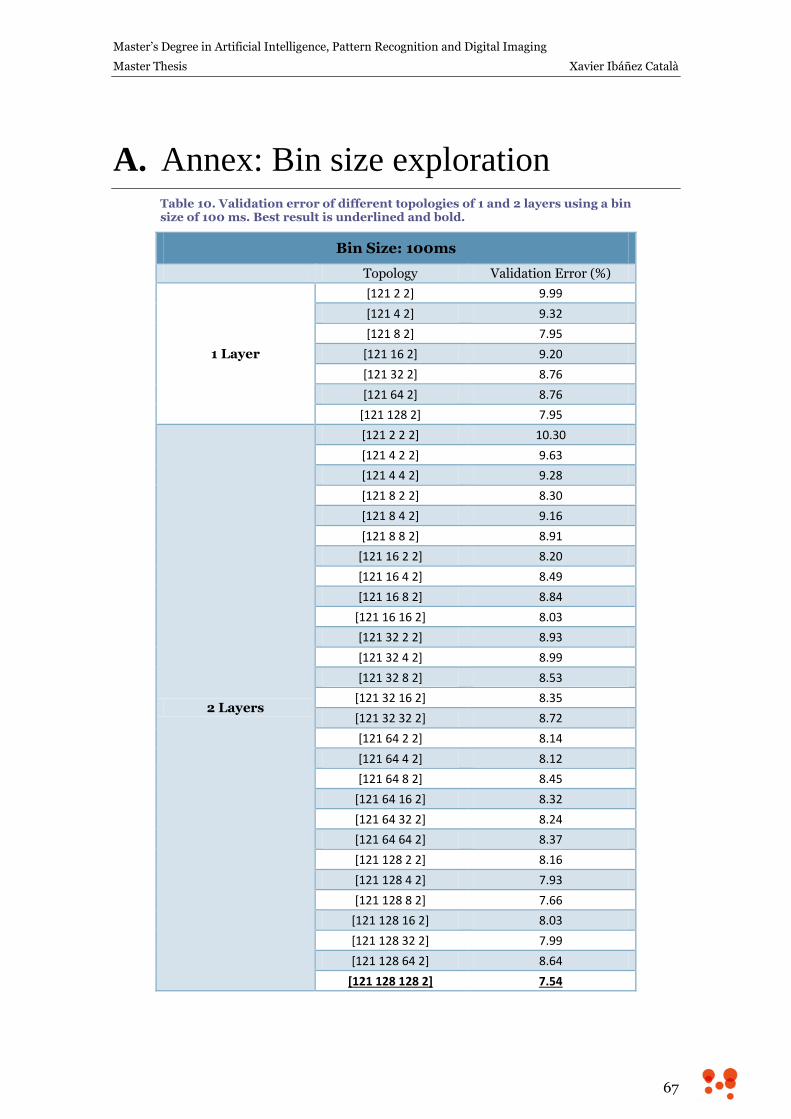
Master’s Degree in Artificial Intelligence, Pattern Recognition and Digital Imaging
Master Thesis Xavier Ibáñez Català
67
A. Annex: Bin size exploration Table 10. Validation error of different topologies of 1 and 2 layers using a bin size of 100 ms. Best result is underlined and bold.
Bin Size: 100ms
Topology Validation Error (%)
1 Layer
[121 2 2] 9.99
[121 4 2] 9.32
[121 8 2] 7.95
[121 16 2] 9.20
[121 32 2] 8.76
[121 64 2] 8.76
[121 128 2] 7.95
2 Layers
[121 2 2 2] 10.30
[121 4 2 2] 9.63
[121 4 4 2] 9.28
[121 8 2 2] 8.30
[121 8 4 2] 9.16
[121 8 8 2] 8.91
[121 16 2 2] 8.20
[121 16 4 2] 8.49
[121 16 8 2] 8.84
[121 16 16 2] 8.03
[121 32 2 2] 8.93
[121 32 4 2] 8.99
[121 32 8 2] 8.53
[121 32 16 2] 8.35
[121 32 32 2] 8.72
[121 64 2 2] 8.14
[121 64 4 2] 8.12
[121 64 8 2] 8.45
[121 64 16 2] 8.32
[121 64 32 2] 8.24
[121 64 64 2] 8.37
[121 128 2 2] 8.16
[121 128 4 2] 7.93
[121 128 8 2] 7.66
[121 128 16 2] 8.03
[121 128 32 2] 7.99
[121 128 64 2] 8.64
[121 128 128 2] 7.54
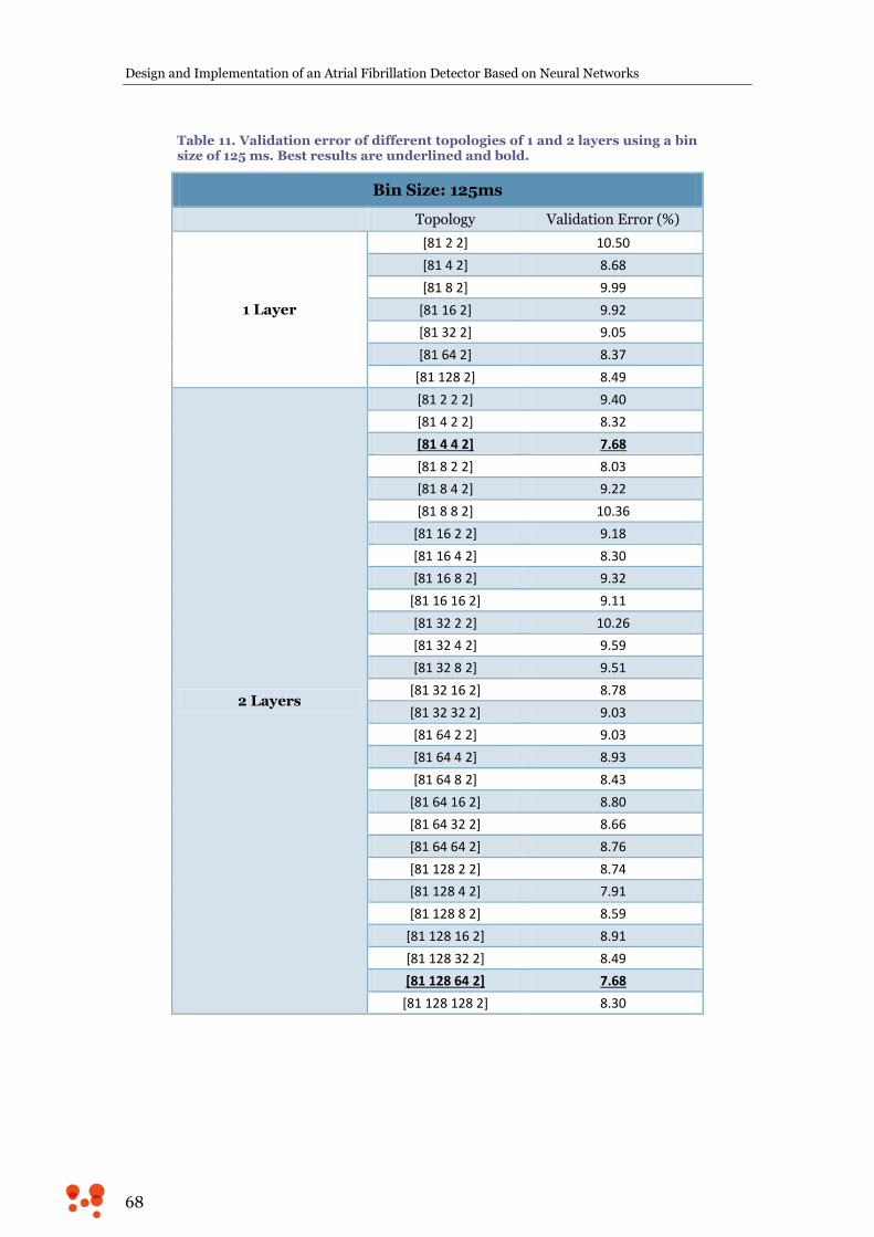
Design and Implementation of an Atrial Fibrillation Detector Based on Neural Networks
68
Table 11. Validation error of different topologies of 1 and 2 layers using a bin size of 125 ms. Best results are underlined and bold.
Bin Size: 125ms
Topology Validation Error (%)
1 Layer
[81 2 2] 10.50
[81 4 2] 8.68
[81 8 2] 9.99
[81 16 2] 9.92
[81 32 2] 9.05
[81 64 2] 8.37
[81 128 2] 8.49
2 Layers
[81 2 2 2] 9.40
[81 4 2 2] 8.32
[81 4 4 2] 7.68
[81 8 2 2] 8.03
[81 8 4 2] 9.22
[81 8 8 2] 10.36
[81 16 2 2] 9.18
[81 16 4 2] 8.30
[81 16 8 2] 9.32
[81 16 16 2] 9.11
[81 32 2 2] 10.26
[81 32 4 2] 9.59
[81 32 8 2] 9.51
[81 32 16 2] 8.78
[81 32 32 2] 9.03
[81 64 2 2] 9.03
[81 64 4 2] 8.93
[81 64 8 2] 8.43
[81 64 16 2] 8.80
[81 64 32 2] 8.66
[81 64 64 2] 8.76
[81 128 2 2] 8.74
[81 128 4 2] 7.91
[81 128 8 2] 8.59
[81 128 16 2] 8.91
[81 128 32 2] 8.49
[81 128 64 2] 7.68
[81 128 128 2] 8.30
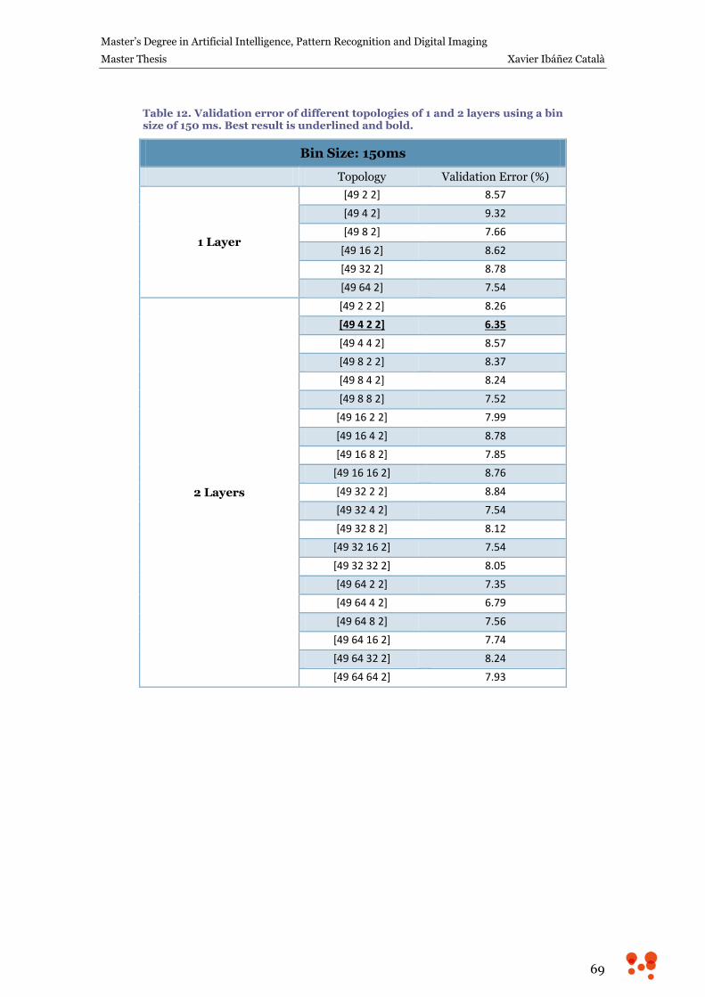
Master’s Degree in Artificial Intelligence, Pattern Recognition and Digital Imaging
Master Thesis Xavier Ibáñez Català
69
Table 12. Validation error of different topologies of 1 and 2 layers using a bin size of 150 ms. Best result is underlined and bold.
Bin Size: 150ms
Topology Validation Error (%)
1 Layer
[49 2 2] 8.57
[49 4 2] 9.32
[49 8 2] 7.66
[49 16 2] 8.62
[49 32 2] 8.78
[49 64 2] 7.54
2 Layers
[49 2 2 2] 8.26
[49 4 2 2] 6.35
[49 4 4 2] 8.57
[49 8 2 2] 8.37
[49 8 4 2] 8.24
[49 8 8 2] 7.52
[49 16 2 2] 7.99
[49 16 4 2] 8.78
[49 16 8 2] 7.85
[49 16 16 2] 8.76
[49 32 2 2] 8.84
[49 32 4 2] 7.54
[49 32 8 2] 8.12
[49 32 16 2] 7.54
[49 32 32 2] 8.05
[49 64 2 2] 7.35
[49 64 4 2] 6.79
[49 64 8 2] 7.56
[49 64 16 2] 7.74
[49 64 32 2] 8.24
[49 64 64 2] 7.93
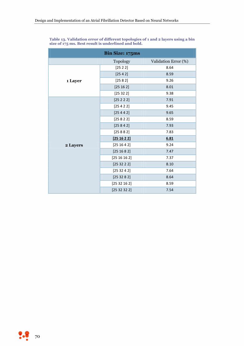
Design and Implementation of an Atrial Fibrillation Detector Based on Neural Networks
70
Table 13. Validation error of different topologies of 1 and 2 layers using a bin size of 175 ms. Best result is underlined and bold.
Bin Size: 175ms
Topology Validation Error (%)
1 Layer
[25 2 2] 8.64
[25 4 2] 8.59
[25 8 2] 9.26
[25 16 2] 8.01
[25 32 2] 9.38
2 Layers
[25 2 2 2] 7.91
[25 4 2 2] 9.45
[25 4 4 2] 9.65
[25 8 2 2] 8.59
[25 8 4 2] 7.93
[25 8 8 2] 7.83
[25 16 2 2] 6.81
[25 16 4 2] 9.24
[25 16 8 2] 7.47
[25 16 16 2] 7.37
[25 32 2 2] 8.10
[25 32 4 2] 7.64
[25 32 8 2] 8.64
[25 32 16 2] 8.59
[25 32 32 2] 7.54
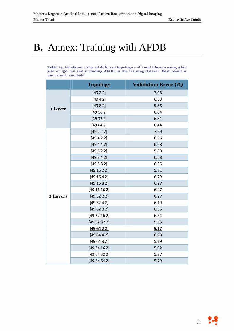
Master’s Degree in Artificial Intelligence, Pattern Recognition and Digital Imaging
Master Thesis Xavier Ibáñez Català
71
B. Annex: Training with AFDB
Table 14. Validation error of different topologies of 1 and 2 layers using a bin size of 150 ms and including AFDB in the training dataset. Best result is underlined and bold.
Topology Validation Error (%)
1 Layer
[49 2 2] 7.08
[49 4 2] 6.83
[49 8 2] 5.56
[49 16 2] 6.04
[49 32 2] 6.31
[49 64 2] 6.44
2 Layers
[49 2 2 2] 7.99
[49 4 2 2] 6.06
[49 4 4 2] 6.68
[49 8 2 2] 5.88
[49 8 4 2] 6.58
[49 8 8 2] 6.35
[49 16 2 2] 5.81
[49 16 4 2] 6.79
[49 16 8 2] 6.27
[49 16 16 2] 6.27
[49 32 2 2] 6.27
[49 32 4 2] 6.19
[49 32 8 2] 6.56
[49 32 16 2] 6.54
[49 32 32 2] 5.65
[49 64 2 2] 5.17
[49 64 4 2] 6.08
[49 64 8 2] 5.19
[49 64 16 2] 5.92
[49 64 32 2] 5.27
[49 64 64 2] 5.79

Design and Implementation of an Atrial Fibrillation Detector Based on Neural Networks
72
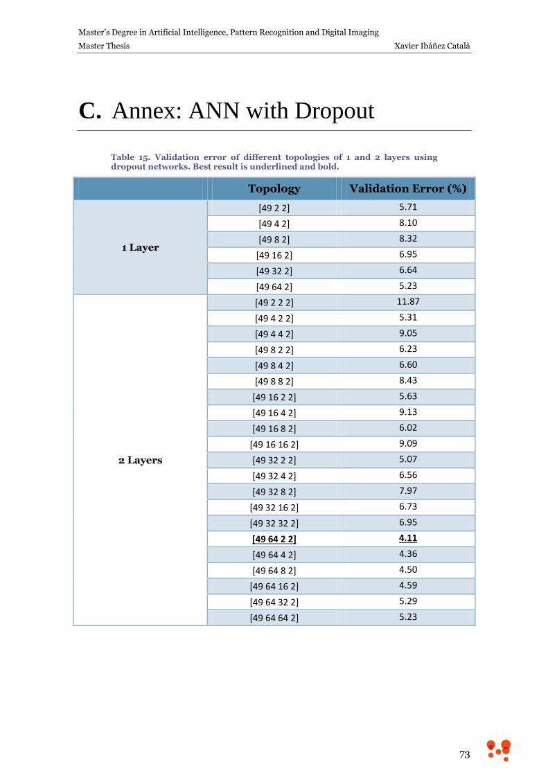
Master’s Degree in Artificial Intelligence, Pattern Recognition and Digital Imaging
Master Thesis Xavier Ibáñez Català
73
C. Annex: ANN with Dropout
Table 15. Validation error of different topologies of 1 and 2 layers using dropout networks. Best result is underlined and bold.
Topology Validation Error (%)
1 Layer
[49 2 2] 5.71
[49 4 2] 8.10
[49 8 2] 8.32
[49 16 2] 6.95
[49 32 2] 6.64
[49 64 2] 5.23
2 Layers
[49 2 2 2] 11.87
[49 4 2 2] 5.31
[49 4 4 2] 9.05
[49 8 2 2] 6.23
[49 8 4 2] 6.60
[49 8 8 2] 8.43
[49 16 2 2] 5.63
[49 16 4 2] 9.13
[49 16 8 2] 6.02
[49 16 16 2] 9.09
[49 32 2 2] 5.07
[49 32 4 2] 6.56
[49 32 8 2] 7.97
[49 32 16 2] 6.73
[49 32 32 2] 6.95
[49 64 2 2] 4.11
[49 64 4 2] 4.36
[49 64 8 2] 4.50
[49 64 16 2] 4.59
[49 64 32 2] 5.29
[49 64 64 2] 5.23