Department of Biological Engineering, Massachusetts

© 2018 The Authors. Open Access chapter published by World Scientific Publishing Company and distributed under the terms of the Creative Commons Attribution Non-Commercial (CC BY-NC) 4.0 License.

Shallow Sparsely-Connected Autoencoders for Gene Set Projection

Maxwell P. Gold, Alexander LeNail, and Ernest Fraenkel Department of Biological Engineering, Massachusetts Institute of Technology, 21 Ames St.

Cambridge, MA, 02139, USA Email: [email protected]

When analyzing biological data, it can be helpful to consider gene sets, or predefined groups of biologically related genes. Methods exist for identifying gene sets that are differential between conditions, but large public datasets from consortium projects and single-cell RNA-Sequencing have opened the door for gene set analysis using more sophisticated machine learning techniques, such as autoencoders and variational autoencoders. We present shallow sparsely-connected autoencoders (SSCAs) and variational autoencoders (SSCVAs) as tools for projecting gene-level data onto gene sets. We tested these approaches on single-cell RNA-Sequencing data from blood cells and on RNA-Sequencing data from breast cancer patients. Both SSCA and SSCVA can recover known biological features from these datasets and the SSCVA method often outperforms SSCA (and six existing gene set scoring algorithms) on classification and prediction tasks.

Keywords: autoencoder, variational autoencoder, single-cell RNA-Sequencing, gene set

1. Introduction

RNA-Sequencing (RNA-Seq) experiments can quantify the RNA expression levels for ~20,000 human genes and this data may reveal differences between experimental conditions, such as cancerous tissue vs. healthy tissue. Typically, RNA-Seq analysis begins with identifying genes with differential RNA levels across conditions and determining if such genes are over-represented in any predefined gene sets (i.e. groups of biologically related genes). This standard approach can be useful but is also quite simplistic; it ignores relationships among the genes and assumes all genes in a gene set are equally important to the group. Consortium projects (such as The Cancer Genome Atlas (TCGA) [1]) and the development of single-cell RNA-Sequencing (scRNA-Seq) [2] have yielded large public datasets for RNA-Seq analysis; this has permitted the use of more complex machine learning techniques, such as autoencoders [3] and variational autoencoders (VAEs) [4], for analyzing those data. These methods can project the high-dimensional gene space onto a lower-dimensional latent space, which may help with visualization, denoising, and/or interpretation [5–7]. Additionally, some neural networks and autoencoders have even been designed to incorporate biological information by using sparsely-connected nodes that only receive inputs from biologically-related genes [8,9]. Many of these neural-network-based and autoencoder-based approaches have focused primarily on increasing accuracy, but recently, groups have used these methods for data interpretation. For example, Way and Greene (2018) used a VAE on TCGA data, wherein they projected RNA-Seq

Pacific Symposium on Biocomputing 2019

374

data onto a reduced latent space, identified nodes that differentiate cancer subtypes, and used the learned model parameters to search for biological significance [10]. Chen et al. (2018) detailed a similar approach, whereby they used sparse connections to project genes onto gene sets and then had a fully-connected layer between the gene set nodes and latent nodes [11]; a gene set was considered meaningful if it had a high input weight into a relevant latent superset node. Here we describe a different approach for using autoencoders for gene set analysis. We present shallow sparsely-connected autoencoders (SSCAs) (Figure 1A) and shallow sparsely-connected variational autoencoders (SSCVAs) (Figure 1B) as tools for projecting gene-level data onto gene sets, wherein those gene set scores can be used for downstream analysis. These methods use a single-layer autoencoder or VAE with sparse connections (representing known biological relationships) in order to attain a value for each gene set. Chen et al. (2018) mentioned the SSCA model (Figure 1A) but did not thoroughly explore its utility for gene set projection [11]. There are many statistical methods for gene set scoring (see Section 2.5), but these techniques often rely on assumptions that do not reflect the underlying biology (e.g. all genes are equally important to a gene set). That being said, the machine-learning approaches presented in this work allow for learning a specific nonlinear mapping function for each gene set; thus, each gene within a gene set can be weighted differently and a single gene can have distinct weights across gene sets. Ideally, the gene set scores should be able to retain high-level information from the gene-level data and provide new insights regarding the relevant gene sets. To test whether the SSCA and SSCVA algorithms can extract such gene set scores, we ran both algorithms on scRNA-Seq data from human blood cells and on RNA-Seq data from patients with breast cancer; we used classification and prediction tasks to compare these new methods to six existing gene set scoring algorithms and assessed the biological interpretability of SSCA and SSCVA by performing differential analysis using the computed scores.

2. Methods

2.1. Model Summary

This work explores shallow sparsely-connected autoencoders (SSCAs) (Figure 1A) and shallow sparsely-connected variational autoencoders (SSCVAs) (Figure 1B). Autoencoders learn an encoder function that projects input data onto a lower dimensional space and a decoder function that aims to recover the input data from the low-dimensional projections. The model is trained by minimizing the reconstruction loss (i.e. some measure of distance between the reconstructed output and the original input). Variational autoencoders (VAEs), however, learn a continuous distribution (typically a multivariate gaussian) to represent the input data. The encoder learns projections onto both a mean vector and a standard deviation vector (which are used to represent a multivariate Gaussian) and the decoder takes samples from the encoded distribution and learns a function to project these samples onto the original space. For VAEs, the model is trained by minimizing both the aforementioned


375

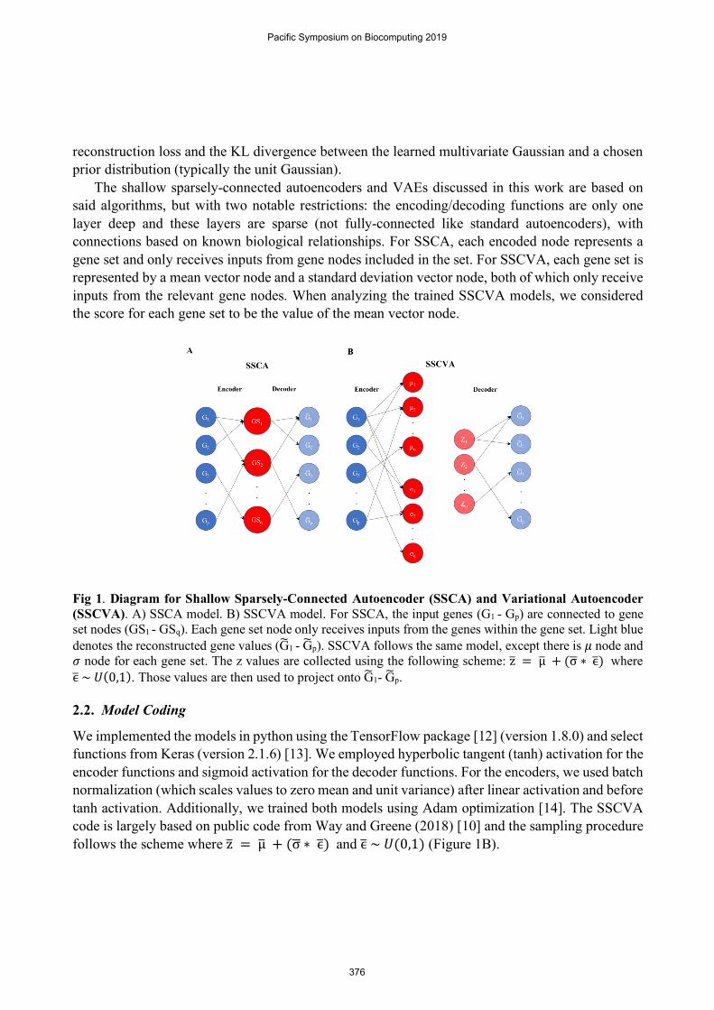
reconstruction loss and the KL divergence between the learned multivariate Gaussian and a chosen prior distribution (typically the unit Gaussian). The shallow sparsely-connected autoencoders and VAEs discussed in this work are based on said algorithms, but with two notable restrictions: the encoding/decoding functions are only one layer deep and these layers are sparse (not fully-connected like standard autoencoders), with connections based on known biological relationships. For SSCA, each encoded node represents a gene set and only receives inputs from gene nodes included in the set. For SSCVA, each gene set is represented by a mean vector node and a standard deviation vector node, both of which only receive inputs from the relevant gene nodes. When analyzing the trained SSCVA models, we considered the score for each gene set to be the value of the mean vector node.

Fig 1. Diagram for Shallow Sparsely-Connected Autoencoder (SSCA) and Variational Autoencoder (SSCVA). A) SSCA model. B) SSCVA model. For SSCA, the input genes (G1 - Gp) are connected to gene set nodes (GS1 - GSq). Each gene set node only receives inputs from the genes within the gene set. Light blue denotes the reconstructed gene values (G!1 - G!p). SSCVA follows the same model, except there is " node and # node for each gene set. The z values are collected using the following scheme: z% = µ% + (σ, ∗ϵ%) where ϵ%~1(0,1). Those values are then used to project onto G!1- G!p.

2.2. Model Coding

We implemented the models in python using the TensorFlow package [12] (version 1.8.0) and select functions from Keras (version 2.1.6) [13]. We employed hyperbolic tangent (tanh) activation for the encoder functions and sigmoid activation for the decoder functions. For the encoders, we used batch normalization (which scales values to zero mean and unit variance) after linear activation and before tanh activation. Additionally, we trained both models using Adam optimization [14]. The SSCVA code is largely based on public code from Way and Greene (2018) [10] and the sampling procedure follows the scheme where z% = µ% + (σ, ∗ ϵ%) and ϵ%~1(0,1) (Figure 1B).


376

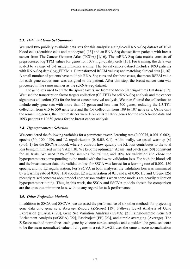
2.3. Data and Gene Set Summary

We used two publicly available data sets for this analysis: a single-cell RNA-Seq dataset of 1078 blood cells (dendritic cells and monocytes) [15] and an RNA-Seq dataset from patients with breast cancer from The Cancer Genome Atlas (TCGA) [1,16]. The scRNA-Seq data matrix consists of preprocessed log TPM values for genes for 1078 high-quality cells [15]. For training, the data was scaled to a range of 0-1 using min-max scaling. The breast cancer dataset includes 1093 patients with RNA-Seq data (log2(FPKM + 1) transformed RSEM values) and matching clinical data [1,16]. A small number of patients have multiple RNA-Seq runs and for these cases, the mean RSEM value for each gene across runs was assigned to the patient. After this step, the breast cancer data was processed in the same manner as the scRNA-Seq dataset. The gene sets used to create the sparse layers are from the Molecular Signatures Database [17]. We used the transcription factor targets collection (C3.TFT) for scRNA-Seq analysis and the cancer signatures collection (C6) for the breast cancer survival analysis. We then filtered the collections to include only gene sets with more than 15 genes and less than 500 genes, reducing the C3.TFT collection from 615 to 550 gene sets and the C6 collection from 189 to 187 gene sets. Using only the remaining genes, the input matrices were 1078 cells x 10992 genes for the scRNA-Seq data and 1093 patients x 10650 genes for the breast cancer analysis.

2.4. Hyperparameter Selection

We considered the following variables for a parameter sweep: learning rate (0.00075, 0.001, 0.002), epochs (50, 100, 150), and L2 regularization (0, 0.05, 0.1). Additionally, we tested warmup (5) (0.05, 1) for the SSCVA model, where 5 controls how quickly the KL loss contributes to the total loss being minimized in the VAE [18]. We kept the optimizer (Adam) and batch size (50) consistent for all trials. We used 90% of the samples for training and 10% for validation and chose the hyperparameters corresponding to the model with the lowest validation loss. For both the blood cell and the breast cancer data, the validation loss for SSCA was lowest for a learning rate of 0.002, 150 epochs, and no L2 regularization. For SSCVA in both analyses, the validation loss was minimized by a learning rate of 0.002, 150 epochs, L2 regularization of 0.1, and 5 of 0.05. Hu and Greene [25] recently raised concerns about model comparison analysis when some models are heavily reliant on hyperparameter tuning. Thus, in this work, the SSCA and SSCVA models chosen for comparison are the ones that minimize loss, without any regard for task performance.

2.5. Other Projection Methods

In addition to SSCA and SSCVA, we assessed the performance of six other methods for projecting gene data onto gene sets: Average Z-score (Z-Score) [19], Pathway Level Analysis of Gene Expression (PLAGE) [20], Gene Set Variation Analysis (GSVA) [21], single-sample Gene Set Enrichment Analysis (ssGSEA) [22], FastProject (FP) [23], and simple averaging (Average). The Z-Score method normalizes each gene by z-score across samples and considers the gene set score to be the mean normalized value of all genes in a set. PLAGE uses the same z-score normalization


377

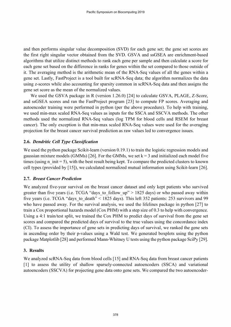
and then performs singular value decomposition (SVD) for each gene set; the gene set scores are the first right singular vector obtained from the SVD. GSVA and ssGSEA are enrichment-based algorithms that utilize distinct methods to rank each gene per sample and then calculate a score for each gene set based on the difference in ranks for genes within the set compared to those outside of it. The averaging method is the arithmetic mean of the RNA-Seq values of all the genes within a gene set. Lastly, FastProject is a tool built for scRNA-Seq data; the algorithm normalizes the data using z-scores while also accounting for sparsity common in scRNA-Seq data and then assigns the gene set score as the mean of the normalized values. We used the GSVA package in R (version 1.26.0) [24] to calculate GSVA, PLAGE, Z-Score, and ssGSEA scores and ran the FastProject program [23] to compute FP scores. Averaging and autoencoder training were performed in python (per the above procedure). To help with training, we used min-max scaled RNA-Seq values as inputs for the SSCA and SSCVA methods. The other methods used the normalized RNA-Seq values (log TPM for blood cells and RSEM for breast cancer). The only exception is that min-max scaled RNA-Seq values were used for the averaging projection for the breast cancer survival prediction as raw values led to convergence issues.

2.6. Dendritic Cell Type Classification

We used the python package Scikit-learn (version 0.19.1) to train the logistic regression models and gaussian mixture models (GMMs) [26]. For the GMMs, we set k = 3 and initialized each model five times (using n_init = 5), with the best result being kept. To compare the predicted clusters to known cell types (provided by [15]), we calculated normalized mutual information using Scikit-learn [26].

2.7. Breast Cancer Prediction

We analyzed five-year survival on the breast cancer dataset and only kept patients who survived greater than five years (i.e. TCGA “days_to_follow_up” > 1825 days) or who passed away within five years (i.e. TCGA “days_to_death” < 1825 days). This left 352 patients: 253 survivors and 99 who have passed away. For the survival analysis, we used the lifelines package in python [27] to train a Cox proportional hazards model (Cox PHM) with a step size of 0.3 to help with convergence. Using a 4:1 train/test split, we trained the Cox PHM to predict days of survival from the gene set scores and compared the predicted days of survival to the true values using the concordance index (CI). To assess the importance of gene sets in predicting days of survival, we ranked the gene sets in ascending order by their p-values using a Wald test. We generated boxplots using the python package Matplotlib [28] and performed Mann-Whitney U tests using the python package SciPy [29].

3. Results

We analyzed scRNA-Seq data from blood cells [15] and RNA-Seq data from breast cancer patients [1] to assess the utility of shallow sparsely-connected autoencoders (SSCA) and variational autoencoders (SSCVA) for projecting gene data onto gene sets. We compared the two autoencoder-


378

based methods to six existing methods for gene set projection (see Methods): GSVA, PLAGE, Z-Score, ssGSEA, FP, and Average.

3.1. Blood scRNA-Seq Analysis

When analyzing scRNA-Seq data, it can be difficult to assess the importance of specific transcription factors (TFs) because mRNA levels do not always correlate with protein abundance [30,31], and TF activity is affected by other factors in the cell, such as chromatin accessibility. One potential solution is to use transcription factor target gene sets (i.e. genes whose expression is potentially affected by a given TF); if the genes regulated by a TF are differential between conditions, this could suggest that the TF is biologically relevant. Thus, in order to explore the scRNA-Seq data set from human blood cells, we performed gene set analysis on 550 transcription factor target gene sets from the Molecular Signatures Database [17]. We performed classification tasks using the gene set encodings to determine whether these projections retain high-level information about the dataset and then analyzed the differential features for biological significance.

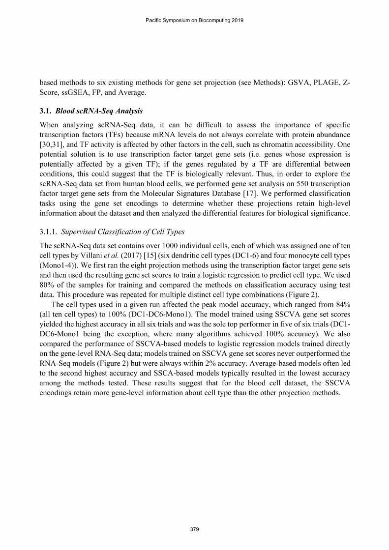
3.1.1. Supervised Classification of Cell Types

The scRNA-Seq data set contains over 1000 individual cells, each of which was assigned one of ten cell types by Villani et al. (2017) [15] (six dendritic cell types (DC1-6) and four monocyte cell types (Mono1-4)). We first ran the eight projection methods using the transcription factor target gene sets and then used the resulting gene set scores to train a logistic regression to predict cell type. We used 80% of the samples for training and compared the methods on classification accuracy using test data. This procedure was repeated for multiple distinct cell type combinations (Figure 2). The cell types used in a given run affected the peak model accuracy, which ranged from 84% (all ten cell types) to 100% (DC1-DC6-Mono1). The model trained using SSCVA gene set scores yielded the highest accuracy in all six trials and was the sole top performer in five of six trials (DC1-DC6-Mono1 being the exception, where many algorithms achieved 100% accuracy). We also compared the performance of SSCVA-based models to logistic regression models trained directly on the gene-level RNA-Seq data; models trained on SSCVA gene set scores never outperformed the RNA-Seq models (Figure 2) but were always within 2% accuracy. Average-based models often led to the second highest accuracy and SSCA-based models typically resulted in the lowest accuracy among the methods tested. These results suggest that for the blood cell dataset, the SSCVA encodings retain more gene-level information about cell type than the other projection methods.


379

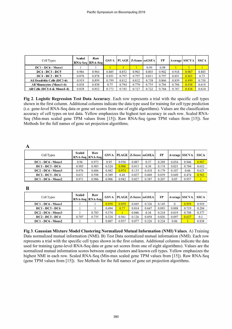
Fig 2. Logistic Regression Test Data Accuracy. Each row represents a trial with the specific cell types shown in the first column. Additional columns indicate the data type used for training for cell type prediction (i.e. gene-level RNA-Seq data or gene set scores from one of eight algorithms). Values are the classification accuracy of cell types on test data. Yellow emphasizes the highest test accuracy in each row. Scaled RNA-Seq (Min-max scaled gene TPM values from [15]). Raw RNA-Seq (gene TPM values from [15]). See Methods for the full names of gene set projection algorithms.

Fig 3. Gaussian Mixture Model Clustering Normalized Mutual Information (NMI) Values. A) Training Data normalized mutual information (NMI). B) Test Data normalized mutual information (NMI). Each row represents a trial with the specific cell types shown in the first column. Additional columns indicate the data used for training (gene-level RNA-Seq data or gene set scores from one of eight algorithms). Values are the normalized mutual information scores between output clusters and known cell types. Yellow emphasizes the highest NMI in each row. Scaled RNA-Seq (Min-max scaled gene TPM values from [15]). Raw RNA-Seq (gene TPM values from [15]). See Methods for the full names of gene set projection algorithms.


380

3.1.2. Unsupervised Clustering of Cell Types

We then examined whether unsupervised clustering of the gene set projections could separate samples by cell type. We trained a Gaussian mixture model on the gene set scores from each method for 80% of the relevant samples and this model was used to predict clusters for the training and test data. In order to evaluate the quality of clustering, we calculated the normalized mutual information (NMI) between the predicted clusters and the known cell types. This procedure was repeated for five distinct groups of three cell types and the results are summarized in Figure 3.

For the training data (Figure 3A), SSCA-based and PLAGE-based models performed best with SSCA-based models having the highest NMI in three cases and PLAGE-based models in two cases. SSCVA-based and GSVA-based models also led to comparatively high NMI scores, while Z-Score-based and Average-based models performed poorly in almost all cases. We observed different results for the test data (Figure 3B), however. The DC1-DC6-Mono1 task led to a tie between the models based on scores from GSVA, PLAGE and SSCVA; on the four remaining tasks, SSCVA-based models and PLAGE-based models each scored highest on two. It is noteworthy that the model trained using SSCVA encodings outperformed the SSCA-based model on the test data, a trend also observed in the logistic regression analysis.

3.1.3. Top Features Detected for SSCVA and SSCA

In addition to retaining high-level information about the samples, gene set projection methods should help identify biologically meaningful gene sets from the data. In order to assess whether these new methods can recover known biology, we performed differential analysis using the gene set scores. The first trial focused on the DC6 cells, which are also known as plasmacytoid dendritic cells [15]. For each of the 550 gene sets, we calculated the median score for all DC6 samples and the median score for all other dendritic cell samples (DC1-5) and ranked the gene sets based on the absolute value of the difference between these medians. We then performed the same analysis comparing all the dendritic cell types (DC1-6) with monocytes (Mono1-4).

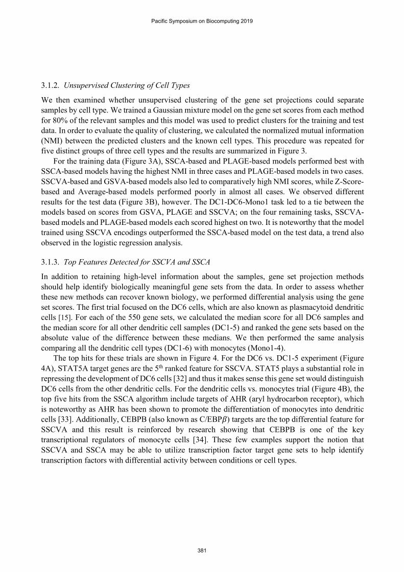
The top hits for these trials are shown in Figure 4. For the DC6 vs. DC1-5 experiment (Figure 4A), STAT5A target genes are the 5th ranked feature for SSCVA. STAT5 plays a substantial role in repressing the development of DC6 cells [32] and thus it makes sense this gene set would distinguish DC6 cells from the other dendritic cells. For the dendritic cells vs. monocytes trial (Figure 4B), the top five hits from the SSCA algorithm include targets of AHR (aryl hydrocarbon receptor), which is noteworthy as AHR has been shown to promote the differentiation of monocytes into dendritic cells [33]. Additionally, CEBPB (also known as C/EBP6) targets are the top differential feature for SSCVA and this result is reinforced by research showing that CEBPB is one of the key transcriptional regulators of monocyte cells [34]. These few examples support the notion that SSCVA and SSCA may be able to utilize transcription factor target gene sets to help identify transcription factors with differential activity between conditions or cell types.


381

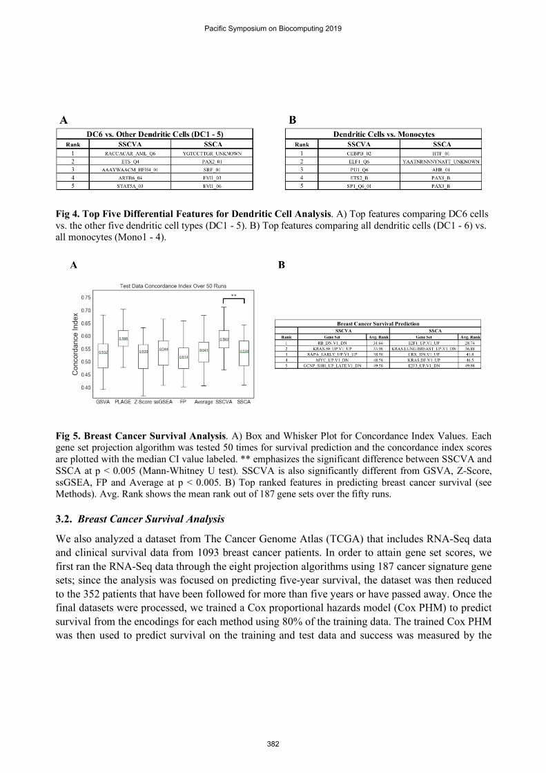
Fig 4. Top Five Differential Features for Dendritic Cell Analysis. A) Top features comparing DC6 cells vs. the other five dendritic cell types (DC1 - 5). B) Top features comparing all dendritic cells (DC1 - 6) vs. all monocytes (Mono1 - 4).

Fig 5. Breast Cancer Survival Analysis. A) Box and Whisker Plot for Concordance Index Values. Each gene set projection algorithm was tested 50 times for survival prediction and the concordance index scores are plotted with the median CI value labeled. ** emphasizes the significant difference between SSCVA and SSCA at p < 0.005 (Mann-Whitney U test). SSCVA is also significantly different from GSVA, Z-Score, ssGSEA, FP and Average at p < 0.005. B) Top ranked features in predicting breast cancer survival (see Methods). Avg. Rank shows the mean rank out of 187 gene sets over the fifty runs.

3.2. Breast Cancer Survival Analysis

We also analyzed a dataset from The Cancer Genome Atlas (TCGA) that includes RNA-Seq data and clinical survival data from 1093 breast cancer patients. In order to attain gene set scores, we first ran the RNA-Seq data through the eight projection algorithms using 187 cancer signature gene sets; since the analysis was focused on predicting five-year survival, the dataset was then reduced to the 352 patients that have been followed for more than five years or have passed away. Once the final datasets were processed, we trained a Cox proportional hazards model (Cox PHM) to predict survival from the encodings for each method using 80% of the training data. The trained Cox PHM was then used to predict survival on the training and test data and success was measured by the


382

concordance index between the actual and predicted days of survival. This was repeated fifty times with distinct training/test splits. When analyzing the Cox PHM predictions on the test data, models for all eight gene set scoring methods showed a wide range of concordance index values across the fifty trials (Figure 5A). PLAGE-based and SSCVA-based models performed best (median concordance index ~0.58), while the other projection methods led to models with a median concordance index of ~0.54. There is no significant difference between the SSCVA and PLAGE results, but SSCVA concordance index values are significantly different than the other six models (p value < 0.005, Mann-Whitney U test). Additionally, each Cox PHM outputs a list of features ranked by their effect on survival (see Methods). We collected this ranked list for each of the fifty models for the SSCA and SSCVA encodings (Figure 5B). For SSCVA, the top ranked feature across the fifty runs is RB_DN.V1_DN and the RB-loss signature (low RB1) is associated with poor disease outcome in breast cancer [35]. Additionally, the top ranked feature for SSCA is E2F1_UP.V1_UP; this result is supported by previous research as well, as E2F1 transcript levels are related to breast cancer outcome [36].

4. Discussion

This work explores shallow sparsely-connected autoencoders (SSCAs) and variational autoencoders (SSCVAs) as methods for projecting RNA-Seq data onto gene sets. When using test data, models trained on the SSCVA encodings often performed as well as the models trained on the gene-level RNA-Seq data and frequently outperformed (or matched) the existing projection algorithms. SSCA-based models, however, performed well on training data, but poorly on test data. These results suggest that the SSCVA encoding space may be better suited to extrapolation than that of SSCA, but future work is necessary to confirm and interpret this trend. Additionally, it is difficult to assess a method’s ability to recover known biology without a ground truth, but we evaluated SSCA and SSCVA on whether differential analysis produced reasonable results. For the blood scRNA-Seq data set, we found the top hits for SSCVA and SSCA included known transcriptional regulators of the groups being tested. Moreover, for the cancer analysis, the top gene sets for both SSCA and SSCVA are cancer signatures related to genes previously associated with breast cancer survival. These observations do not prove that SSCA and SSCVA can uncover insightful biology in all situations, but it is encouraging that the methods identify known features in the data sets tested. Compared to the other methods discussed, the shallow sparsely-connected autoencoder framework provides greater flexibility for modeling biological phenomena. For instance, if a transcription factor acts as both an activator and a repressor, any given target gene may be up or downregulated. The averaging-based methods (Z-Score, FP, and Average) may miss this trend because the combination of high and low values can reduce the signal. Additionally, the averaging-based approaches and the enrichment-based approaches (ssGSEA and GSVA) both weight all genes equally within a gene set, despite the fact some genes may be more relevant to the gene set than others. PLAGE addresses this issue by learning a specific mapping for each gene set, but the algorithm is limited to finding a linear combination of gene values. SSCA and SSCVA, however,


383

can learn specific nonlinear mappings for each gene set, which could be useful for modeling complex biological relationships. Moreover, the mapping functions learned by SSCA and SSCVA can potentially provide more information about the importance of genes within specific gene sets. Further exploration is required to better understand the utility of these models for single-cell omics data sets. For instance, SSCVAs may be particularly useful for analysis of cellular differentiation. Variational autoencoders are designed to produce an encoding space where clusters are distinguishable, but close together, and this can result in smooth transitions between groups of samples; thus, the SSCVA scores can potentially be leveraged for identification and visualization of gene sets that transition in importance throughout differentiation. Additionally, this framework could potentially be applied to other gene-associated omics types, such as methylation. Unfortunately, a weakness of autoencoder-based methods is that the results may not be entirely consistent between runs; the other six methods tested yield the same result every time, but since autoencoders are initialized randomly each trial, the learned encoder function (and thus the gene set scores) may not be identical across runs. This observation has also been noted by Chen et al. (2018) [11] and we are currently exploring whether changes in activation functions, hyperparameters, and/or regularization can improve consistency, while maintaining classification accuracy. Overall this work supports the use of SSCA and SSCVA for gene set analysis on large RNA-Seq data sets. These methods still require more rigorous testing and evaluation, and future work on this project will be dedicated to improving consistency between runs and understanding situations and data types where SSCA and/or SSCVA may be particularly useful.

Acknowledgements

This work was supported by NIH grants R01NS089076 and 1U01CA18498. We would like to thank the PSB reviewers for their thoughtful comments and helpful suggestions and also want to acknowledge Ludwig Schmidt for informative conversations regarding the models.

References

1. Weinstein, J. N., Collisson, E. a, Mills, G. B., Shaw, K. R. M., Ozenberger, B. a, Ellrott, K., Shmulevich, I., Sander, C. & Stuart, J. M. Nat. Genet. 45, 1113 (2013).

2. Tang, F., Barbacioru, C., Wang, Y., Nordman, E., Lee, C., Xu, N., Wang, X., Bodeau, J., Tuch, B. B., Siddiqui, A., Lao, K. & Surani, M. A. Nat. Methods 6, 377 (2009).

3. Liou, C. Y., Huang, J. C. & Yang, W. C. in Neurocomputing 71, 3150 (2008). 4. Kingma, D. P. & Welling, M. Ppt (2013). doi:10.1051/0004-6361/201527329 5. žurauskiene, J. & Yau, C. BMC Bioinformatics 17, (2016). 6. Xie, R., Wen, J., Quitadamo, A., Cheng, J. & Shi, X. BMC Genomics 18, (2017). 7. Wang, Y., Solus, L., Dai Yang, K. & Uhler, C. ArXiv Prepr. arXiv 1705.10220 (2017). 8. Lin, C., Jain, S., Kim, H. & Bar-Joseph, Z. Nucleic Acids Res. 45, (2017). 9. Kang, T., Ding, W., Zhang, L., Ziemek, D. & Zarringhalam, K. BMC Bioinformatics 18,

(2017).


384

10. Way, G. P. & Greene, C. S. Pac. Symp. Biocomput. 23, 80 (2018). 11. Chen, H.-I., Chiu, Y.-C., Zhang, T., Zhang, S., Huang, Y. & Chen, Y. ArXiv e-prints

(2018). 12. Abadi, M. et al. (2015). 13. Chollet, F. GitHub (2015). Available at: https://github.com/fchollet/keras. 14. Kingma, D. & Ba, J. arXiv Prepr. arXiv1412.6980 1 (2014).

doi:10.1109/ICCE.2017.7889386 15. Villani, A.-C. et al. Science (80-. ). 356, eaah4573 (2017). 16. Grossman, R. L., Heath, A. P., Ferretti, V., Varmus, H. E., Lowy, D. R., Kibbe, W. A. &

Staudt, L. M. N. Engl. J. Med. (2016). doi:10.1056/NEJMp1607591 17. Subramanian, A., Tamayo, P., Mootha, V. K., Mukherjee, S., Ebert, B. L., Gillette, M. a,

Paulovich, A., Pomeroy, S. L., Golub, T. R., Lander, E. S. & Mesirov, J. P. Proc. Natl. Acad. Sci. U. S. A. 102, 15545 (2005).

18. Sønderby, C. K., Raiko, T., Maaløe, L., Sønderby, S. K. & Winther, O. Nips 48, (2016). 19. Lee, E., Chuang, H. Y., Kim, J. W., Ideker, T. & Lee, D. PLoS Comput. Biol. 4, (2008). 20. Tomfohr, J., Lu, J. & Kepler, T. B. BMC Bioinformatics 6, (2005). 21. Hänzelmann, S., Castelo, R., Guinney, J., Kim, S. C., Seo, Y. J., Chung, W., Eum, H. H.,

Nam, D.-H., Kim, J., Joo, K. M. & Park, W.-Y. BMC Bioinformatics 14, 7 (2013). 22. Barbie, D. A. et al. Nature 462, 108 (2009). 23. DeTomaso, D. & Yosef, N. BMC Bioinformatics 17, (2016). 24. Sonja, H., Castelo, R. & Guinney, J. Bioconductor.org 1 (2014). 25. Hu, Q. & Greene, C. S. bioRxiv (2018). 26. Pedregosa, F., Varoquaux, G., Gramfort, A., Michel, V., Thirion, B., Grisel, O., Blondel,

M., Prettenhofer, P., Weiss, R., Dubourg, V., Vanderplas, J., Passos, A., Cournapeau, D., Brucher, M., Perrot, M. & Duchesnay, E. J. Mach. Learn. Res. 12, 2825 (2011).

27. Davidson-Pilon, C. et al. (2018). doi:10.5281/zenodo.1252342 28. Hunter, J. D. Comput. Sci. Eng. (2007). doi:10.1109/MCSE.2007.55 29. Oliphant, T. E. Comput. Sci. Eng. (2007). doi:10.1109/MCSE.2007.58 30. Lundberg, E., Fagerberg, L., Klevebring, D., Matic, I., Geiger, T., Cox, J., Älgenäs, C.,

Lundeberg, J., Mann, M. & Uhlen, M. Mol. Syst. Biol. (2010). doi:10.1038/msb.2010.106 31. Vogel, C. & Marcotte, E. M. Nat. Rev. Genet. (2012). doi:10.1038/nrg3185 32. Esashi, E., Wang, Y. H., Perng, O., Qin, X. F., Liu, Y. J. & Watowich, S. S. Immunity 28,

509 (2008). 33. Goudot, C., Coillard, A., Villani, A. C., Gueguen, P., Cros, A., Sarkizova, S., Tang-Huau,

T. L., Bohec, M., Baulande, S., Hacohen, N., Amigorena, S. & Segura, E. Immunity 47, 582 (2017).

34. Huber, R., Pietsch, D., Panterodt, T. & Brand, K. Cellular Signalling 24, 1287 (2012). 35. Ertel, A., Dean, J. L., Rui, H., Liu, C., Witkiewicz, A., Knudsen, K. E. & Knudsen, E. S.

Cell Cycle 9, 4153 (2010). 36. Hallett, R. M. & Hassell, J. A. BMC Res Notes 4, 95 (2011).


385

Documents

Department of Biological Engineering, Massachusetts