DEPARTMENT OF CHEMICAL ENGINEERING LABORATORY FOR …

DEPARTMENT OF CHEMICAL ENGINEERING

LABORATORY FOR THE PREPARATION OF NANO AND MICROMATERIALS

PK: Characterization of Nanoparticles by Dynamic and Static Light Scattering Technique

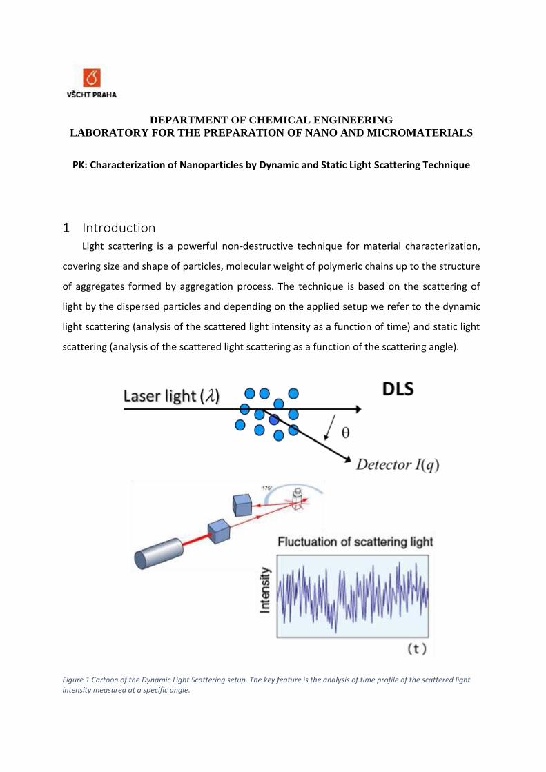
1 Introduction Light scattering is a powerful non-destructive technique for material characterization,

covering size and shape of particles, molecular weight of polymeric chains up to the structure

of aggregates formed by aggregation process. The technique is based on the scattering of

light by the dispersed particles and depending on the applied setup we refer to the dynamic

light scattering (analysis of the scattered light intensity as a function of time) and static light

scattering (analysis of the scattered light scattering as a function of the scattering angle).

Figure 1 Cartoon of the Dynamic Light Scattering setup. The key feature is the analysis of time profile of the scattered light intensity measured at a specific angle.

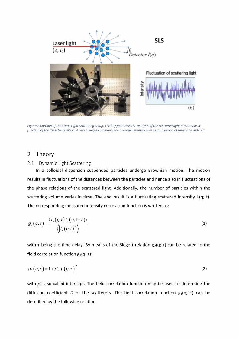
Figure 2 Cartoon of the Static Light Scattering setup. The key feature is the analysis of the scattered light intensity as a function of the detector position. At every angle commonly the average intensity over certain period of time is considered.

2 Theory

2.1 Dynamic Light Scattering

In a colloidal dispersion suspended particles undergo Brownian motion. The motion

results in fluctuations of the distances between the particles and hence also in fluctuations of

the phase relations of the scattered light. Additionally, the number of particles within the

scattering volume varies in time. The end result is a fluctuating scattered intensity Is(q; t).

The corresponding measured intensity correlation function is written as:

2 2

, , t,

,

s s

s

I q t I qg q

I q t

(1)

with being the time delay. By means of the Siegert relation g2(q; ) can be related to the

field correlation function g1(q; ):

2

2 1, 1 ,g q g q (2)

with is so-called intercept. The field correlation function may be used to determine the

diffusion coefficient D of the scatterers. The field correlation function g1(q; ) can be

described by the following relation:

2

2 2

1ln , ...2

vcg q Dq Dq (3)

where D is the intensity weighted diffusion coefficient, cv is the coefficient of variation

related to the sample polydispersity. Using the Stokes-Einstein equation and the viscosity of

the surrounding medium the radius can be calculated:

6

Bh

k TR

D (4)

2.2 Static Light Scattering

In static light scattering experiments the intensity of light scattered due to the presence

of objects (scatterers) with refractive index different from the surrounding medium is

measured as a function of the scattering angle, . This angle is directly related to the

modulus of the scattering vector 4 sin 2q , by the wavelength . In the simplest

case of monodispersed spherical particles the average scattered intensity Is(q) is proportional

to the particle form factor P(q) as follows

2

0( ) ( )pI q I CNV P q (5)

where I0 is the incident light intensity, C is the instrument constant which is a function of the

experimental setup and N is the number of particles with a volume Vp. In the case of

monodisperse particles with diameter substantially smaller that the laser wavelength P(q)

can be calculate analytically as follows:

2

3

3 sin cosp p p

p

qR qR qRP q

qR

(6)

with Rp being the particle radius.

Since the size of particles is a priory not known, commonly a Guinier plot is used to extract

the particles size. The Guinier Plot allows the determination of the Radius of Gyration (Rg)

from the measured scattered intensity Is(q) as a function of the scattering angle θ. It is used

in X-Ray, neutron and static light scattering (SLS). Using a logarithmic plot of the Guinier

equation

2

2ln ln 03

s g

qI q I R (7)

where Rg can be simple obtained from the slope of the liner fit of the ln Is(q) vs. q2/3

3 Aims The goals of this lab include the following:

(a) Analyze the size of particles synthesized either by emulsion polymerization or

precipitation methods.

(b) Compare the size obtained by dynamic and static light scattering technique

(c) Investigate the impact of salt concentration on the measured size and stability of

obtained particles.

4 Pre-lab preparation Read the laboratory protocol carefully to understand the procedure. Furthermore get

familiar with the instrument setup and controlling software.

5 Experimental Procedure

5.1 Materials and methods

Chemicals: Deionized water

Sodium Chloride (NaCl), MW: 58.44 g/mol

Particle suspension prepared either by emulsion polymerization or precipitation

method

Apparatus: Beakers (50 ml)

Pipets (200 L and 1 mL)

Balance

5.2 Precautions and safety information

(i) Safety first! Personal protective equipment (lab coats, gloves, goggles, shoes that

cover the entire feet: no slippers or sandals allowed) should be worn at all times

when in the lab and when handling all chemicals.

(ii) information (Source: Sigma Aldrich material safety data sheet) regarding all

reagents used in this lab is as follows:

Chemical Signal word Symbol

NaCl No toxicity data available

Prevention is better than cure!

(iii) Before starting the experiments, ensure all glassware are clean, contamination can

alter the results of your hard work.

Work Procedure

1. Prepare a solution of nanoparticle suspension in water. Use 50 mL of deionized water into

which you add 200 L of original particle suspension.

2. Transfer 2 mL of this diluted suspension of particles to the measurement cuvette and

clean its outer part with the paper tissue.

3. Insert cuvette into the device goniometer and select either Dynamic or Static Light

Scattering mode. No for should be spplied when inserting the cuvette into the goniometer!

It could cause damage of the instrument. Please follow closely the manual or ask the

laboratory instructor.

4. Analyze the prepared samples and record the measured values of particle size as well as

polydispersity.

Evaluation and Report preparation guidelines

This work is supporting the previous step where students prepared particles either by emulsion

polymerization or by precipitation. Therefore obtained results will be part of the report for

these two works. Protocols including sizes of the prepared particles as well as trends as a

function of the condition will be provided not later than 1 week after characterization

laboratory described in this document.

Postlab questions

1. Which methods for particle characterization do you know?

2. What is the difference between static and dynamic light scattering? How the measurement

is done using both techniques?

3. How to calculate hydrodynamic radius and radius of gyration? What is the difference

between them?

4. What is the impact of the salt on the size of particles?

Good luck!

Appendix – Extract from Instruction Manual to the LS Instrument

device

4 LS Spectrometer software

Version: 6.3 to 6.6 If an older version is installed on your system you might ask LS Instruments for an update.

4.1 Structure of the main program

This section explains in detail the structure and functionality of the LS Spectrometer software

provided with the instrument. The graphical user interface is organized into 3 different sections

as shown in Fig. 4.1.

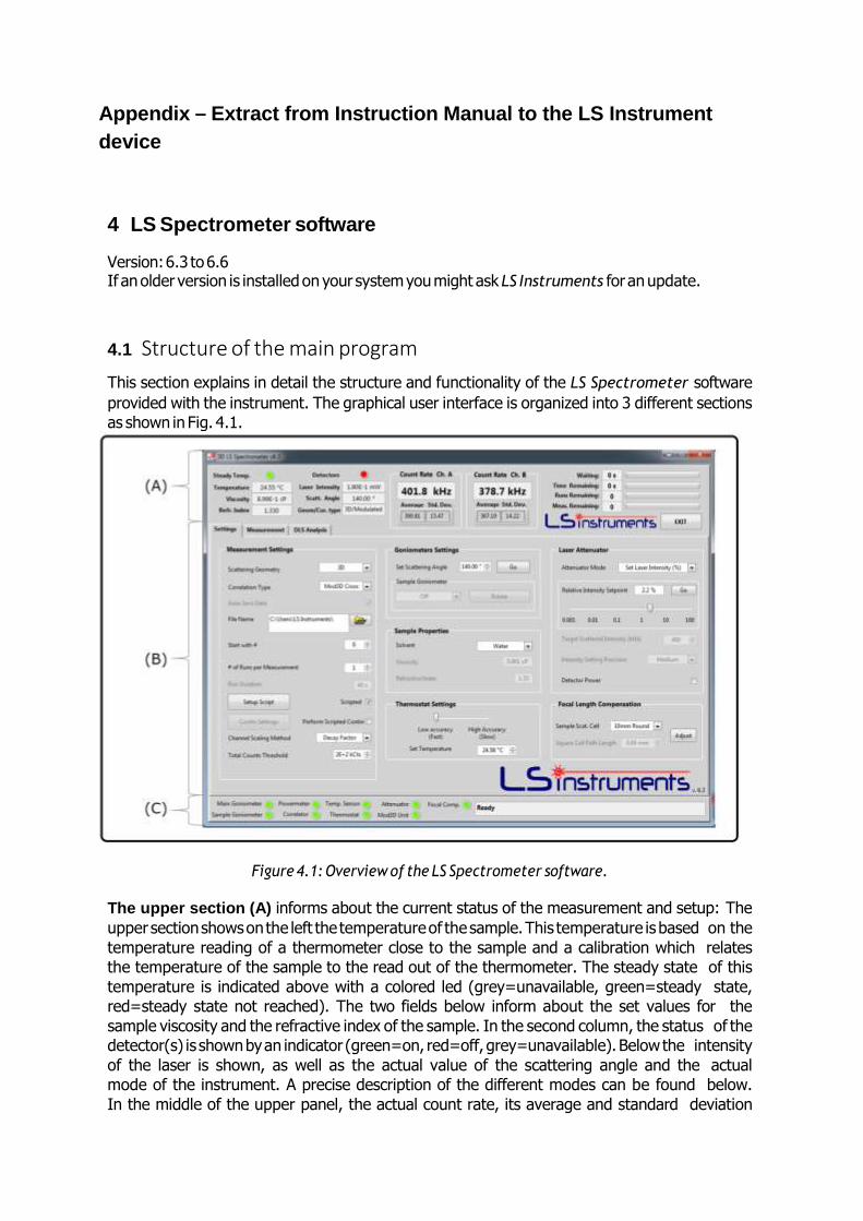
Figure 4.1: Overview of the LS Spectrometer software.

The upper section (A) informs about the current status of the measurement and setup: The

upper section shows on the left the temperature of the sample. This temperature is based on the

temperature reading of a thermometer close to the sample and a calibration which relates

the temperature of the sample to the read out of the thermometer. The steady state of this

temperature is indicated above with a colored led (grey=unavailable, green=steady state,

red=steady state not reached). The two fields below inform about the set values for the

sample viscosity and the refractive index of the sample. In the second column, the status of the

detector(s) is shown by an indicator (green=on, red=off, grey=unavailable). Below the intensity

of the laser is shown, as well as the actual value of the scattering angle and the actual

mode of the instrument. A precise description of the different modes can be found below.

In the middle of the upper panel, the actual count rate, its average and standard deviation

are shown for both channel separately (if second detector is installed). On the right the timing of

the current measurements are indicated. Also the main exit button is located here (Please use

only the exit button and not the cross button in the top right corner of the program to exit

the) The middle section (B) is divided into three tabs, Settings, Measurement and DLS Analysis:

This section contains all the software controlled settings of the LS Spectrometer. Depending on

the hardware configuration and options installed, certain parts are grayed out. The settings are

divided into three columns. On the left, measurement settings, in the center the goniometer

settings and on the right the laser attenuator settings can be adjusted.

The lower section (C) informs about the initialization and status of the hardware and the

software:

When the software starts it initializes sequentially all the available options, the corresponding

status is indicated by a colored led for each option and details are provided in the status text

field on the right. Options which are not available remain grayed-out. A correctly functioning

option turns to green after the initialization, while options that fail to initialize are indicated by a red led. When the initialization process is finished, Ready is displayed in the text field on the

right.

4.1.1 Measurement settings

Scattering geometry Here one can select the scattering geometry, which can be either 2D or

3D. In section 3.5 the switching between scattering geometries is explained. Upon the setting

change the software will show a small animation illustrating the required corresponding hardware

operations. The different options of the selected scattering geometry can be selected in the pull

down menu below. For each scattering geometry, there are different correlation types available.

The available correlation types depend on the options you have installed and the actual selected

scattering geometry.

5.3 Scattering geometry and correlation type

1. auto: The auto-correlation is the standard correlation mode. In this mode a single APD is

used and the correlation function is calculated auto correlating the corresponding signal.

2. pseudo (optional requiring two APD): In this mode of measurement, the signals of both

APDs are correlated. It is only available in the 2D scattering geometry. The pseudo cross

mode suppresses after pulsing which has a particularly negative effect on the measurement

of small particles. For more information study section 1.

3. 3D Cross (optional requiring 3D option): The 3D cross correlation mode is required for

turbid samples to suppress multiple scattering. For more information study section 1 and

2.

4. Mod3D Cross (optional requiring the 3D and the modulation option): Further

improvement of the 3D cross-correlation mode. For more information study section 1

and 2.

Auto save data The “auto save data” option, if checked, allows automated saving of the

recorded data while measurements are performed. Click on the folder icon and chose the folder

path where you want your data to be saved and a base file name. Consecutive measurements

will be saved in different files having the specified base name followed by running number. The

first number of this running number can be specified on the main panel of the measurement

settings.

Number of runs per measurement and run duration The length of a measurement can

be defined by two numbers. One is the duration per run and the other is the number of runs

per measurement. The total duration of one measurement is thus the number of runs times

the duration per run. The splitting of one measurement into several runs has the advantage of

allowing to assess the stability of each measurement.

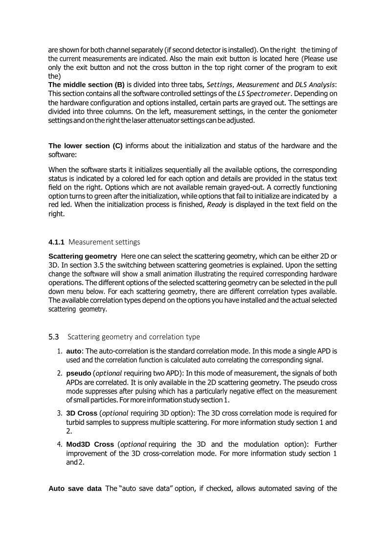
Setup script The script window is very useful if several measurements in a row should be

conducted. A screen shot of the script window is shown in Fig. 4.2. The upper line, “New Set”, is

the line which can be edited. It contains the lowest angle and the highest angle of the series of

measurement, the angular step size , the number of measurements and its duration as well as the

waiting time in between each run and the temperature. Note that depending on the angular step

size the last measurement will be at a lower angle than the highest specified angle. For

example: lowest angle 20 degree, highest angle 135 degree and step size 10 degree would lead

to an highest angle in this series of 130 degree. Once the parameters are set, you may click on

”Insert line” to include the line just prepared in the script.

All sets of runs are shown as a list in the middle of the window. If you would like to delete a line

click on it and select ”Delete line”. It is not possible to directly edit a line in the main window.

On the right panel, the estimated time for the script to be completed is shown.

If this time is unexpectedly large, check the number of runs per measurement as this influences

the total script time.

The buttons ”Load script”and ”Save Script”enable you to save and load scripts. The lower panel in

this window shows the file name and location as well as the start number added to the files for

auto saved data. Once the script is configured, you may click on the OK button to return to

the main window.

Figure 4.2: Overview of scripted window.

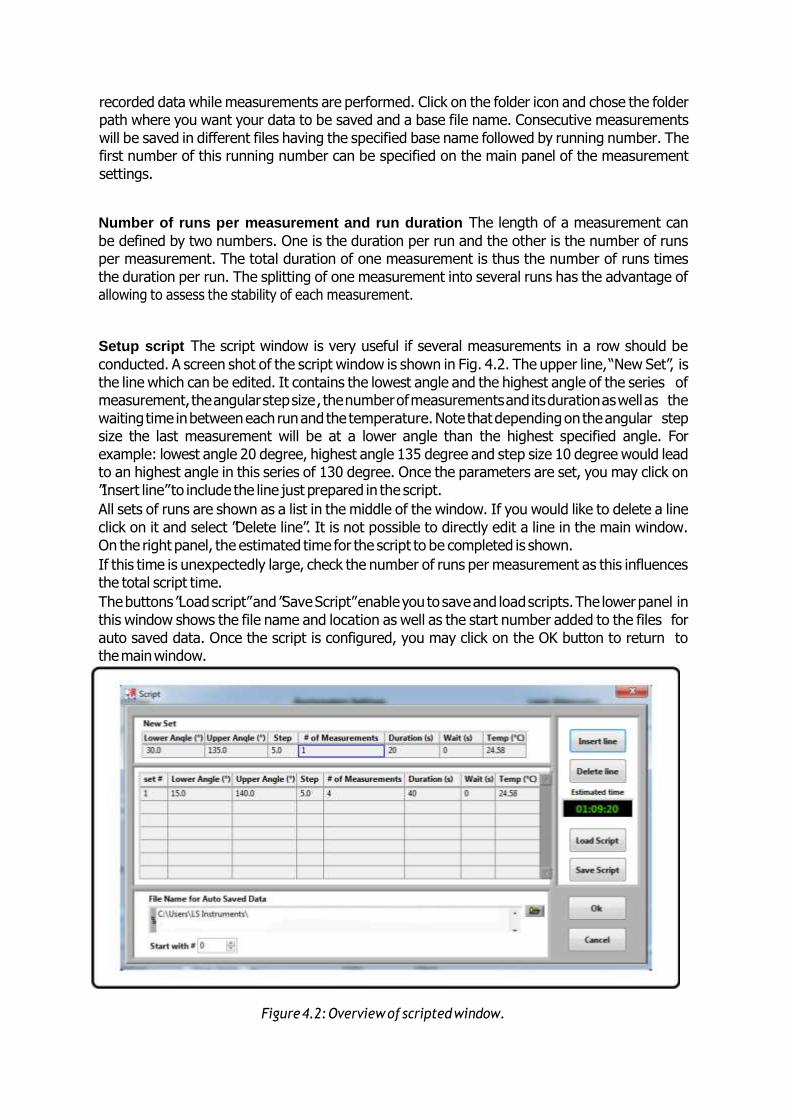
CONTIN settings Within a scripted measurement, CONTIN [10] analysis can be performed

automatically. If ticked, the settings of the CONTIN analysis can be adapted. The according

window is shown in Fig. 4.3. As explained in section 4.1.8 the scattering model, the type of

boundary selection, and the number of nodes can be selected. Additionally, the definition of

the baseline can be adjusted. This is adjusted in terms of number of channels starting from

the highest available channel. For more information on the other parameters please study

section 4.1.8.

Figure 4.3: Overview of scripted CONTIN analysis settings.

Channel scaling method When performing measurements on the same sample but at different

angles, the measured correlation function shifts along the lag time abscissa. This can cause

problems for the cumulant analysis fit. To avoid this issue you can apply lag time scaling. Upon

an angle change, the software will try to guess an optimal channel interval for the new angle

depending on the chosen channel scaling method.

1. No scaling: No scaling is applied. The maximum lag time for the fit is constant for all

measurements.

2. q squared: The adjustment of the maximum lag time follows from that of the previous

angle by the theoretical q2 law. Details on setting the maximum lag time are described in

section 4.1.7.

3. Decay factor: The adjustment of the maximum lag time is based on the decay of the

g2 function. The maximum lag time is thus set at the lag time where the correlation

function decreases from the minimum set lag time by a given percentage which can be

fixed by the user. Details on setting the decay factor are described in section 4.1.7.

Total counts threshold This value is used for the cumulant analysis performed during the

measurement. A minimum number of counts is required to perform a cumulant analysis with a

meaningful result. The total counts threshold fixes this threshold.

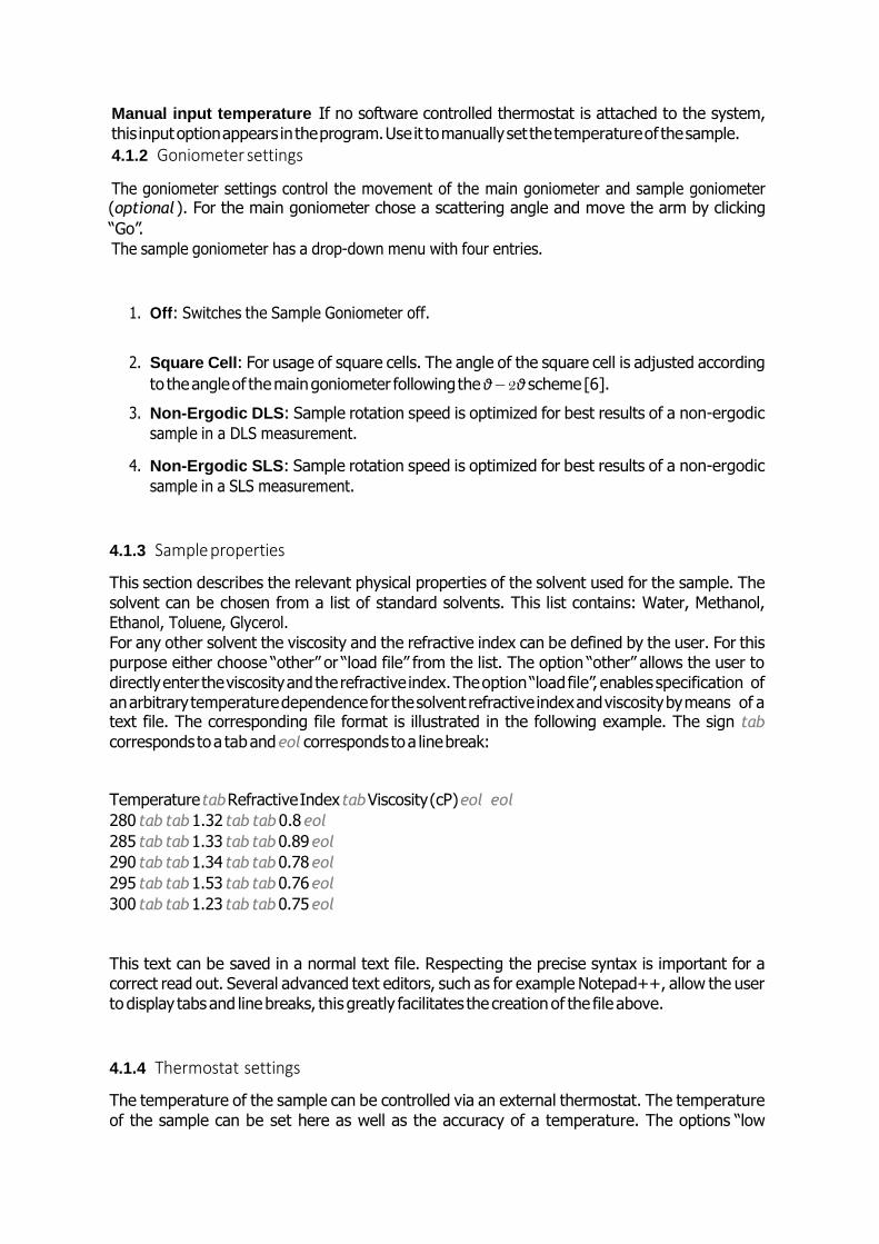
Manual input temperature If no software controlled thermostat is attached to the system,

this input option appears in the program. Use it to manually set the temperature of the sample.

4.1.2 Goniometer settings

The goniometer settings control the movement of the main goniometer and sample goniometer (optional ). For the main goniometer chose a scattering angle and move the arm by clicking

“Go”.

The sample goniometer has a drop-down menu with four entries.

1. Off: Switches the Sample Goniometer off.

2. Square Cell: For usage of square cells. The angle of the square cell is adjusted according

to the angle of the main goniometer following the θ − 2θ scheme [6].

3. Non-Ergodic DLS: Sample rotation speed is optimized for best results of a non-ergodic

sample in a DLS measurement.

4. Non-Ergodic SLS: Sample rotation speed is optimized for best results of a non-ergodic

sample in a SLS measurement.

4.1.3 Sample properties

This section describes the relevant physical properties of the solvent used for the sample. The

solvent can be chosen from a list of standard solvents. This list contains: Water, Methanol,

Ethanol, Toluene, Glycerol.

For any other solvent the viscosity and the refractive index can be defined by the user. For this

purpose either choose “other” or “load file” from the list. The option “other” allows the user to

directly enter the viscosity and the refractive index. The option “load file”, enables specification of

an arbitrary temperature dependence for the solvent refractive index and viscosity by means of a text file. The corresponding file format is illustrated in the following example. The sign tab

corresponds to a tab and eol corresponds to a line break:

Temperature tab Refractive Index tab Viscosity (cP) eol eol

280 tab tab 1.32 tab tab 0.8 eol





This text can be saved in a normal text file. Respecting the precise syntax is important for a

correct read out. Several advanced text editors, such as for example Notepad++, allow the user

to display tabs and line breaks, this greatly facilitates the creation of the file above.

4.1.4 Thermostat settings

The temperature of the sample can be controlled via an external thermostat. The temperature

of the sample can be set here as well as the accuracy of a temperature. The options “low

accuracy” and“high accuracy” define when the temperature will be considered sufficiently stable

for a measurement. Higher accuracy of course imply larger equilibration times.

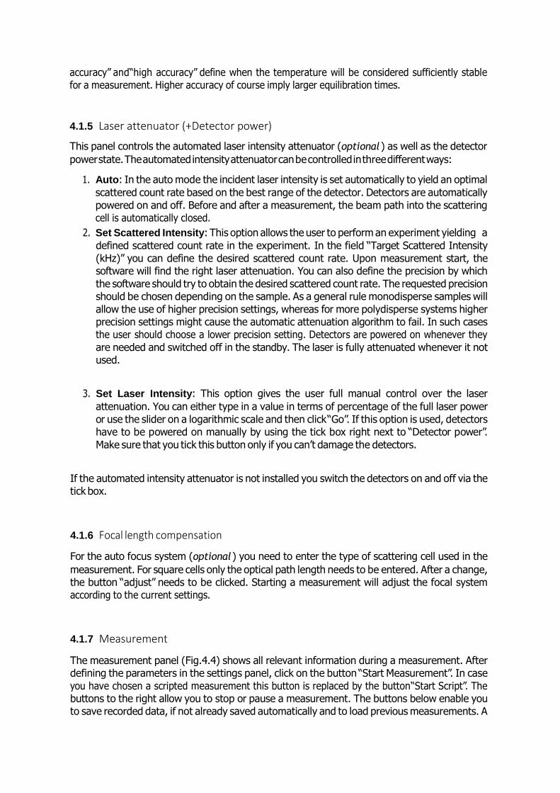
4.1.5 Laser attenuator (+Detector power)

This panel controls the automated laser intensity attenuator (optional ) as well as the detector

power state. The automated intensity attenuator can be controlled in three different ways:

1. Auto: In the auto mode the incident laser intensity is set automatically to yield an optimal

scattered count rate based on the best range of the detector. Detectors are automatically

powered on and off. Before and after a measurement, the beam path into the scattering

cell is automatically closed.

2. Set Scattered Intensity: This option allows the user to perform an experiment yielding a

defined scattered count rate in the experiment. In the field “Target Scattered Intensity

(kHz)” you can define the desired scattered count rate. Upon measurement start, the

software will find the right laser attenuation. You can also define the precision by which

the software should try to obtain the desired scattered count rate. The requested precision

should be chosen depending on the sample. As a general rule monodisperse samples will

allow the use of higher precision settings, whereas for more polydisperse systems higher

precision settings might cause the automatic attenuation algorithm to fail. In such cases

the user should choose a lower precision setting. Detectors are powered on whenever they

are needed and switched off in the standby. The laser is fully attenuated whenever it not

used.

3. Set Laser Intensity: This option gives the user full manual control over the laser

attenuation. You can either type in a value in terms of percentage of the full laser power

or use the slider on a logarithmic scale and then click“Go”. If this option is used, detectors

have to be powered on manually by using the tick box right next to “Detector power”.

Make sure that you tick this button only if you can’t damage the detectors.

If the automated intensity attenuator is not installed you switch the detectors on and off via the

tick box.

4.1.6 Focal length compensation

For the auto focus system (optional ) you need to enter the type of scattering cell used in the

measurement. For square cells only the optical path length needs to be entered. After a change,

the button “adjust” needs to be clicked. Starting a measurement will adjust the focal system

according to the current settings.

4.1.7 Measurement

The measurement panel (Fig.4.4) shows all relevant information during a measurement. After

defining the parameters in the settings panel, click on the button “Start Measurement”. In case

you have chosen a scripted measurement this button is replaced by the button“Start Script”. The

buttons to the right allow you to stop or pause a measurement. The buttons below enable you

to save recorded data, if not already saved automatically and to load previous measurements. A

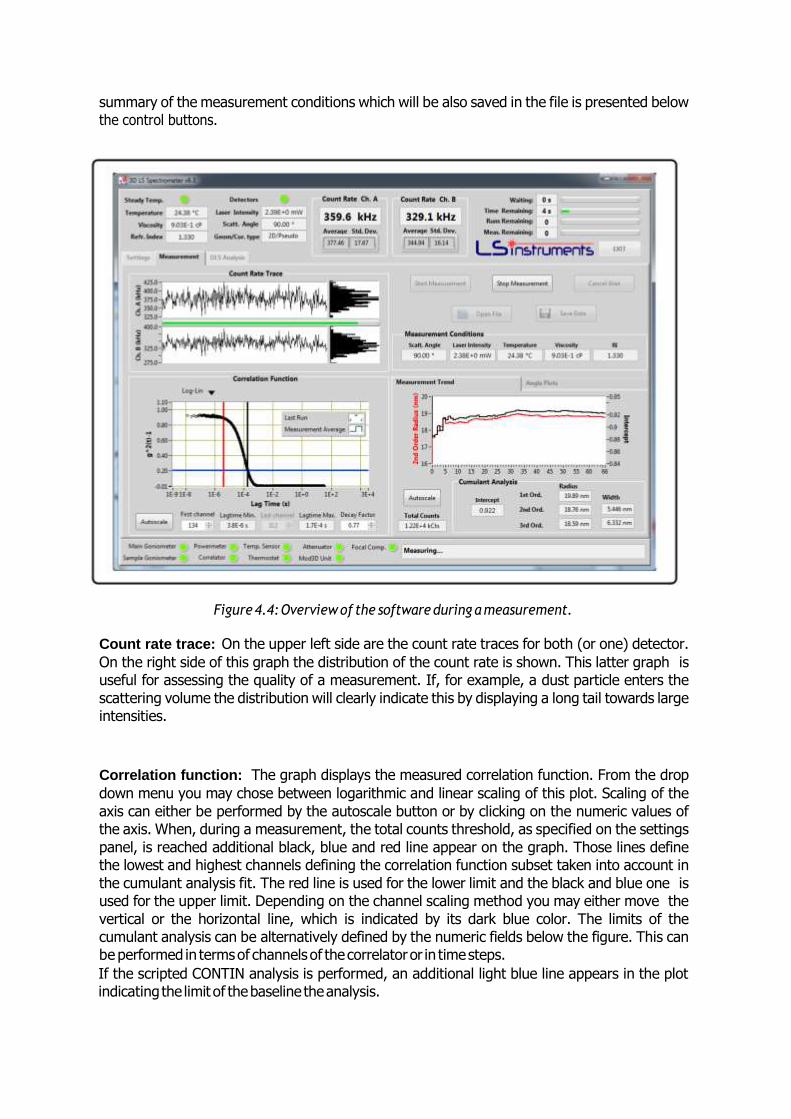
summary of the measurement conditions which will be also saved in the file is presented below

the control buttons.

Figure 4.4: Overview of the software during a measurement.

Count rate trace: On the upper left side are the count rate traces for both (or one) detector.

On the right side of this graph the distribution of the count rate is shown. This latter graph is

useful for assessing the quality of a measurement. If, for example, a dust particle enters the

scattering volume the distribution will clearly indicate this by displaying a long tail towards large

intensities.

Correlation function: The graph displays the measured correlation function. From the drop

down menu you may chose between logarithmic and linear scaling of this plot. Scaling of the

axis can either be performed by the autoscale button or by clicking on the numeric values of

the axis. When, during a measurement, the total counts threshold, as specified on the settings

panel, is reached additional black, blue and red line appear on the graph. Those lines define

the lowest and highest channels defining the correlation function subset taken into account in

the cumulant analysis fit. The red line is used for the lower limit and the black and blue one is

used for the upper limit. Depending on the channel scaling method you may either move the

vertical or the horizontal line, which is indicated by its dark blue color. The limits of the

cumulant analysis can be alternatively defined by the numeric fields below the figure. This can

be performed in terms of channels of the correlator or in time steps.

If the scripted CONTIN analysis is performed, an additional light blue line appears in the plot

indicating the limit of the baseline the analysis.

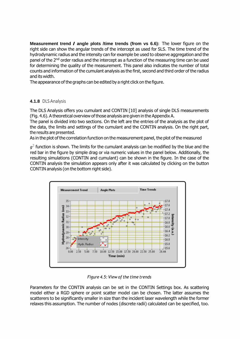
Measurement trend / angle plots /time trends (from vs 6.6): The lower figure on the

right side can show the angular trends of the intercept as used for SLS. The time trend of the

hydrodynamic radius and the intensity can for example be used to observe aggregation and the

panel of the 2nd order radius and the intercept as a function of the measuring time can be used

for determining the quality of the measurement. This panel also indicates the number of total

counts and information of the cumulant analysis as the first, second and third order of the radius

and its width.

The appearance of the graphs can be edited by a right click on the figure.

4.1.8 DLS Analysis

The DLS Analysis offers you cumulant and CONTIN [10] analysis of single DLS measurements

(Fig. 4.6). A theoretical overview of those analysis are given in the Appendix A.

The panel is divided into two sections. On the left are the entries of the analysis as the plot of

the data, the limits and settings of the cumulant and the CONTIN analysis. On the right part,

the results are presented.

As in the plot of the correlation function on the measurement panel, the plot of the measured

g2 function is shown. The limits for the cumulant analysis can be modified by the blue and the

red bar in the figure by simple drag or via numeric values in the panel below. Additionally, the

resulting simulations (CONTIN and cumulant) can be shown in the figure. In the case of the

CONTIN analysis the simulation appears only after it was calculated by clicking on the button

CONTIN analysis (on the bottom right side).

Figure 4.5: View of the time trends

Parameters for the CONTIN analysis can be set in the CONTIN Settings box. As scattering

model either a RGD sphere or point scatter model can be chosen. The latter assumes the

scatterers to be significantly smaller in size than the incident laser wavelength while the former

relaxes this assumption. The number of nodes (discrete radii) calculated can be specified, too.

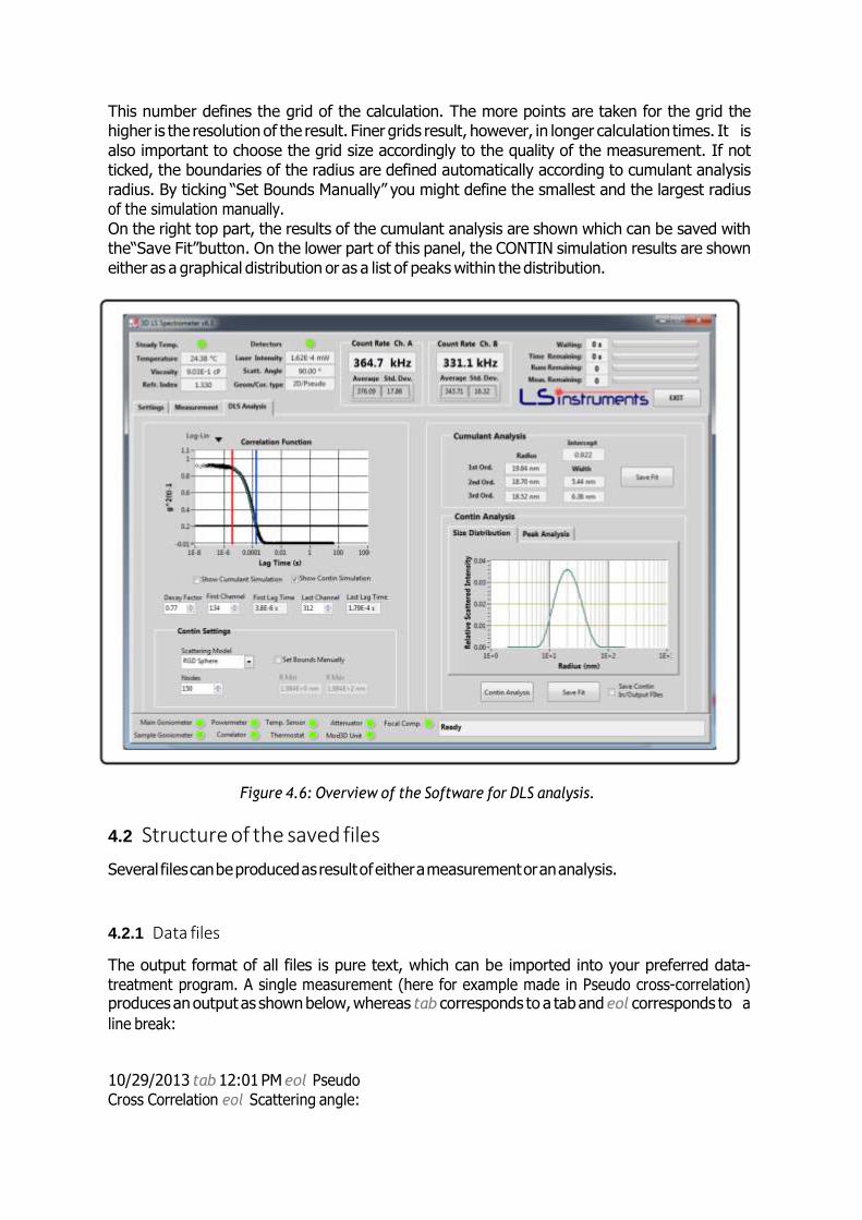
This number defines the grid of the calculation. The more points are taken for the grid the

higher is the resolution of the result. Finer grids result, however, in longer calculation times. It is

also important to choose the grid size accordingly to the quality of the measurement. If not

ticked, the boundaries of the radius are defined automatically according to cumulant analysis

radius. By ticking “Set Bounds Manually” you might define the smallest and the largest radius

of the simulation manually.

On the right top part, the results of the cumulant analysis are shown which can be saved with

the“Save Fit”button. On the lower part of this panel, the CONTIN simulation results are shown

either as a graphical distribution or as a list of peaks within the distribution.

Figure 4.6: Overview of the Software for DLS analysis.

4.2 Structure of the saved files

Several files can be produced as result of either a measurement or an analysis.

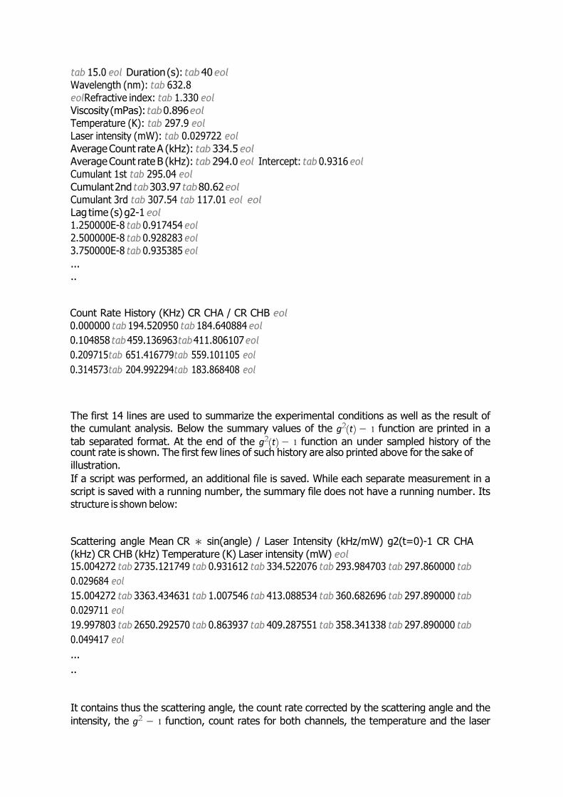
4.2.1 Data files

The output format of all files is pure text, which can be imported into your preferred data-

treatment program. A single measurement (here for example made in Pseudo cross-correlation) produces an output as shown below, whereas tab corresponds to a tab and eol corresponds to a

line break:

10/29/2013 tab 12:01 PM eol Pseudo

Cross Correlation eol Scattering angle:

tab 15.0 eol Duration (s): tab 40 eol

Wavelength (nm): tab 632.8

eolRefractive index: tab 1.330 eol

Viscosity (mPas): tab 0.896 eol

Temperature (K): tab 297.9 eol

Laser intensity (mW): tab 0.029722 eol

Average Count rate A (kHz): tab 334.5 eol

Average Count rate B (kHz): tab 294.0 eol Intercept: tab 0.9316 eol

Cumulant 1st tab 295.04 eol

Cumulant 2nd tab 303.97 tab 80.62 eol

Cumulant 3rd tab 307.54 tab 117.01 eol eol

Lag time (s) g2-1 eol

1.250000E-8 tab 0.917454 eol

2.500000E-8 tab 0.928283 eol

3.750000E-8 tab 0.935385 eol

...

..

Count Rate History (KHz) CR CHA / CR CHB eol

0.000000 tab 194.520950 tab 184.640884 eol

0.104858 tab 459.136963tab 411.806107 eol

0.209715tab 651.416779tab 559.101105 eol

0.314573tab 204.992294tab 183.868408 eol

The first 14 lines are used to summarize the experimental conditions as well as the result of the cumulant analysis. Below the summary values of the g2(t) − 1 function are printed in a

tab separated format. At the end of the g2(t) − 1 function an under sampled history of the count rate is shown. The first few lines of such history are also printed above for the sake of

illustration.

If a script was performed, an additional file is saved. While each separate measurement in a

script is saved with a running number, the summary file does not have a running number. Its

structure is shown below:

Scattering angle Mean CR ∗ sin(angle) / Laser Intensity (kHz/mW) g2(t=0)-1 CR CHA

(kHz) CR CHB (kHz) Temperature (K) Laser intensity (mW) eol 15.004272 tab 2735.121749 tab 0.931612 tab 334.522076 tab 293.984703 tab 297.860000 tab

0.029684 eol

15.004272 tab 3363.434631 tab 1.007546 tab 413.088534 tab 360.682696 tab 297.890000 tab

0.029711 eol

19.997803 tab 2650.292570 tab 0.863937 tab 409.287551 tab 358.341338 tab 297.890000 tab

0.049417 eol

...

..

It contains thus the scattering angle, the count rate corrected by the scattering angle and the

intensity, the g2 − 1 function, count rates for both channels, the temperature and the laser

intensity. Note: Scaling of the intensity by measured laser intensity is only performed in case of an installed automatic intensity attenuator (optional ).

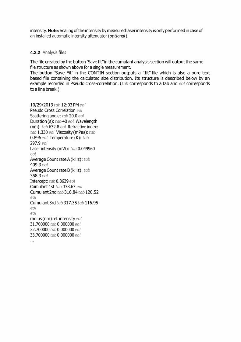
4.2.2 Analysis files

The file created by the button ”Save fit” in the cumulant analysis section will output the same

file structure as shown above for a single measurement.

The button ”Save Fit” in the CONTIN section outputs a ”.fit” file which is also a pure text

based file containing the calculated size distribution. Its structure is described below by an example recorded in Pseudo cross-correlation. (tab corresponds to a tab and eol corresponds

to a line break.)

10/29/2013 tab 12:03 PM eol

Pseudo Cross Correlation eol

Scattering angle: tab 20.0 eol

Duration (s): tab 40 eol Wavelength

(nm): tab 632.8 eol Refractive index:

tab 1.330 eol Viscosity (mPas): tab

0.896 eol Temperature (K): tab

297.9 eol

Laser intensity (mW): tab 0.049960 eol

Average Count rate A (kHz) :tab

409.3 eol

Average Count rate B (kHz): tab

358.3 eol

Intercept: tab 0.8639 eol

Cumulant 1st tab 338.67 eol

Cumulant 2nd tab 316.84 tab 120.52 eol

Cumulant 3rd tab 317.35 tab 116.95 eol eol

radius (nm) rel. intensity eol

31.700000 tab 0.000000 eol

32.700000 tab 0.000000 eol

33.700000 tab 0.000000 eol

...

Documents

DEPARTMENT OF CHEMICAL ENGINEERING LABORATORY FOR …