Department of Commerce

University of Calcutta

Study Material

Cum

Lecture Notes

Only for the Students of M.Com. (Semester IV)-2020

University of Calcutta

(Internal Circulation)

Dear Students,

Hope you, your parents and other family members are safe and secured. We are going

through a world-wide crisis that seriously affects not only the normal life and economy

but also the teaching-learning process of our University and our department is not an

exception.

As the lock-down is continuing and it is not possible to reach you face to face class

room teaching. Keeping in mind the present situation, our esteemed teachers are trying

their level best to reach you through providing study material cum lecture notes of

different subjects. This material is not an exhaustive one though it is an indicative so

that you can understand different topics of different subjects. We believe that it is not the

alternative of direct teaching learning.

It is a gentle request you to circulate this material only to your friends those who are

studying in Semester IV (2020).

Stay safe and stay home.

Best wishes.

Paper CC 402:

Strategic Cost and Management Accounting

(SCM)

1

Strategic cos

CC 402

STRATEGIC COST AND MANAGEMENT ACCOUNTING

MODULE I Unit 1: Introduction

According to the Institute of Cost and works Accountants of India (ICWAI), Management Accounting is ‘a system

of collection and presentation of relevant economic information relating to an enterprise for planning, controlling

and decision-making’.

One of the most comprehensive definitions of Management Accounting given by the International Federation of

Accountants (IFAC) is ‘the process of identification, measurement, accumulation, analysis, preparation,

interpretation and communication of information both financial and operating used by management to plan,

evaluate and control within the organization and to assure use of and accountability for its resources’.

Therefore, management accounting identifies, measures, accumulates, analyses, prepares, interprets and

communicates both financial and non-financial information to the management in performing its functions

effectively.

Strategic management accounting helps formulating superior strategies by providing relevant information to the

management.

Unit 2: Tools of Strategic Cost Management

a) Activity-based Costing b) Life Cycle Costing c) Target Costing d) Quality Costing

a) Activity-based Costing (ABC) Accurate cost information is required for different strategic decision making. It has become much relevant in a

highly competitive globalised business environment. Activity based costing helps apportioning overhead, which is

gradually increasing now-a-days, properly tracing the costs to the products/services.

Traditional Cost Systems vs. ABC

Traditional systems measure accurately volume-related resources like direct labour, materials, energy and

machine-related costs. However, many support activities such as material handling, material procurement, set-

2

ups, production scheduling, etc. are not volume related. Traditional volume based product cost systems, which

assume that products consume all resources in proportion to their production volumes, thus report distorted

product costs.

On the other hand, under ABC system it is considered that activities cause costs and that products (and

customers) create the demands for the activities. ABC system recognizes that businesses must understand the

factors that drive each major activity, the cost of activities and how activities relate to products.

Activities may be classified into three major categories that drive expenses at the product level. They are Unit-

related activities, Batch-related activities and Product-sustaining activities.

Unit-related activities are performed each time a unit of the product is produced.

Batch-related activities are performed each time a batch of goods is produced, e.g., setting up a machine.

Product-sustaining activities are performed to support different products in the product line.

One additional expense category that cannot be directly attributed to individual products may be identified as

Facility-sustaining activities. They are performed to sustain a facility’s general manufacturing process.

FACTORS INFLUENCING APPLICATION OF ABC

In case of high volume of overhead expenditure and product diversity or complexity involving different

activities in different proportions, the cost ascertainment under traditional costing system may be

misleading. ABC system would help tracing costs more accurately linking costs with the activities that drive

such costs.

ACTIVITY BASED MANAGEMENT

ABC analysis may reveal true costs; hence, true profitability of the products, and management may take

appropriate actions to increase the profitability. Some of the actions that may be taken to increase the

profitability are:

Reprice products

Substitute products

Redesign products

Improve processes and operations strategy

Technology investment

Eliminate products The actions mentioned above, if implemented successfully, will reduce the resources required to manufacture

products and to provide service to the customers.

Example 1. Product I Product II

3

Production (units) 50 100 Inspection per product line 25 5 Machine hours per unit 15 20 Total budgeted inspection costs Rs. 33,000 What is the inspection cost per unit under traditional system and ABC system?

Solution:

(a) Machine hour rate: Rs.33000 / (50 x 15 + 100 x 20) = Rs.12

Product I Product II Machine hours worked 50 x 15 = 750 100 x 20 = 2000 Inspection cost @ Rs. 12 per hour 9,000 24,000 Units produced 50 100 Inspection cost per unit 9000/50 = 180 24000/100 = 240

(b) Cost per inspection: Total inspection costs / No. of inspections = 33,000 / 30 = 1,100 Product I Product II

No. of inspections per product line 25 5 Inspection costs @ 1,100 (Rs.) 27,500 5,500 Units produced 50 100 Inspection costs per unit (Rs.) 550 55

Example 2: A company produces two products: X and Y. Both the products are produced on

the same equipment and use the similar processes. Consider the following data.

Machine hrs Direct Labour Actual output No. of Purchase No. of

Per unit hours per unit (units) orders set-ups

Product X 2 4 1000 80 40

Product Y 2 4 10000 160 60

Cost of the activities:

Soln. Volume-related Rs. 1,10,000; Purchase-related Rs. 1,20,000; Set-up-related Rs. 2,10,000

(a) Traditional System: Cost center allocated costs : 110000 + 120000 + 210000 = 4,40,000 Machine hour rate: 440000/(1000 x 2 + 10000 x 2) = Rs. 20 Direct labour hour rate: 440000/(1000 x 4 + 10000 x 4) = Rs. 10 Overhead costs per unit of--

X: Rs. 20 X 2 or Rs. 10 x 4 = Rs.40 Y: Rs. 20 X 2 or Rs. 10 x 4 = Rs.40

Total costs allocated – X: 1000 units x 40 = 40,000; Y: 10000 x 40 = 4,00,000

(b) ABC System: Activities

Volume-related Purchasing-related Set-up-related Costs traced to activities(Rs.) 1,10,000 1,20,000 2,10,000

4

Consumption of activities 22000 240 100 set-ups (cost drivers) mach. hrs. purchase orders Cost per unit of consumption (Rs.) 5 500 2100 Cost traced to products: X (1000 units) 2000x5=10000 80x500=40000 40x2100=84000 Y (10000 units) 20000x5=100000 160x500=80000 60x2100=126000

Overhead cost per unit: X = (10000 + 40000 + 84000)/1000 = 134 Y = (100000 + 80000 + 126000)/10000 = 30.60

b) Life Cycle Costing Life Cycle Costing aims at cost ascertainment of a product over its projected life. It is a system that traces and accumulates the actual costs and revenues attributable to cost object from its introduction to its abandonment. It is also known as cradle-to-grave costing and womb-to-tomb costing which conveys the meaning of fully capturing all costs associated with the product from its initial to final stages, from initial R&D on a product to when customer servicing and support is no longer offered for the product. Phases in Product Life Cycle: The four phases in the product Life Cycle are — (a) Introduction (b) Growth (c) Maturity and (d) Decline. Importance of Life Cycle Costing

Life cycle costing involves tracing of costs and revenues of each product over their life cycle. Costs and revenues can analysed by time periods. The total magnitude of costs for each individual product can be reported and compared with product revenues generated in various time periods.

Life Cycle Costing focuses on recognizing both production and non-production costs. Non-production costs like R&D; design; marketing; distribution; customer service etc. as well as all production costs are considered in Life Cycle Costing.

Based on a more accurate and realistic assessment ot revenues and costs over the life cycle of a product, better cost control / cost reduction decisions, pricing decisions, etc. can be taken.

Life Cycle Costing provides scope for analysis of long term picture of product line profitability, feedback on the effectiveness of life cycle planning and cost data to clarify the economic impact of alternatives chosen in the design, engineering phase etc.

Example:

Year 1 (Rs.)

Year 2 (Rs.)

Year 3 (Rs.) Year 4 (Rs.) Total (Rs.)

(a) Pre-production costs: R&D, Design, etc.

1000 -- -- -- 1000

(b) Manufacturing Costs 1000 2000 3000 1100 7050

(c) Marketing, Distribution, After-sales service costs

200 500 700 50 1500

(d) End of life costs -- -- -- 50 50

(e) Production and Sales (units)

200 500 1000 50 1750

(f) Year-wise total costs (Rs.) [a+b+c+d]

2200 2500 3700 1200 9600

Year-wise per unit costs [f / e]

11.00 5.00 3.70 24.00

Life Cycle Costs per unit (Rs.) [Total costs over the life cycle / total production over the life cycle]

9600/ 1750 = 5.486

5

C) Target Costing

Target Costing is defined as a structured approach in determining the cost at which a proposed product with specified functionality and quality must be produced, to generate a desired level of profitability at its anticipated selling price. Target Costing is a device to continuously control and reduce costs, and manage profit over the life cycle of a product. Target Costing initiates cost management at the earliest stages of product development and applies it throughout the product life cycle by actively involving the entire value chain. Under traditional costing system, Expected Selling Price = Estimated Cost + Required Profit But under Target Costing System, Target Cost = Target Selling Price – Target or Required Profit. If it is found that the product cannot be manufactured at the target costs, initiatives will be required to achieve the target costs through applying different cost control and cost reduction techniques. Value engineering and value analysis may be used to identify innovative and cost effective product features in the planning and concept stages. Design may be changed for reduction of costs. Steps in Target Costing Target Costing is viewed as a part of an overall Profit Management Process, rather than simply a tool for cost Reduction and Cost Management.

The customer requirements as to the functionality and quality of the product are to be ascertained.

The design of the product based on customer’s tastes, expectations and requirements is to be specified. However the need to provide improved products, without significant increase in prices, should be recognized as charging a higher price may not be possible in competitive conditions.

The Target Selling Price is to be determined considering offers of competitors, product utility, prices, target sales volume, etc.

Since profitability is critical for survival, a Target Profit Margin is to be established.

The difference between the Target Selling Price and Target Profit Margin indicates the “Allowable Cost” for the product. Ideally, the Allowable Cost becomes the “Target Cost for the product”. However, the Target Cost may exceed the Allowable Cost, in light of the realities associated with existing capacities and capabilities.

The “Current Costs” for producing the product is to be estimated.

The difference between Current Cost and Target Cost indicates the required cost reduction. The total target is broken down into its various components, each component is studied and opportunities for cost reductions are identified. These activities are referred to as a) Value Engineering (VE) and b) Value Analysis (VA).

Illustration A manufacturing company, operating at 50% of its capacity, manufactures its products at Rs. 1500 per unit (60% variable) and sells its product at Rs. 2000 per unit. Due to competition, its competitors are likely to reduce price by 10%. The company wants to respond aggressively by reducing price by 25% and expects that the present volume of 1,00,000 units p.a. will increase to 2,00,000. The company wants to earn a 20% target profit on sales. Determine Target Cost per unit and prepare a Target Product Profitability Statement. Solution: Particulars Existing Total Production and Sales (units) 100000 Total Costs per unit (Rs.) 1500 Total Sales (Rs.) 20,00,00,000 Total Costs (Rs.) 15,00,00,000 Total Profit (Rs.) 5,00,00,000

6

Particulars Target Total Production and Sales (units) 200000 Target Selling Price per unit (Rs.) 1500 Total Profit per unit (Rs.) [20% of Rs.1500] 300 Target Cost per unit 1200 [Target S.P. – Target Profit] Target Product Profitability Statement Total Per unit Total Sales (Rs.) 30,00,00,000 1500 Total Costs (Rs.) 24,00,00,000 1200 Total Profit (Rs.) 6,00,00,000 300 d) Quality Costing Quality costs are the aggregate of costs of maintaining quality and costs for not maintaining quality. Total quality costs can be classified initially into two categories: Conformance Costs (costs of maintaining quality) and Non-conformance Costs (costs for not maintaining quality). Conformance costs may be classified into two: Prevention Costs and Appraisal Costs Non-conformance costs may be classified into two: Internal Failure Costs and External Failure Costs. Impact of external failure costs is the highest as it will lead to dissatisfaction of the customers, loss of goodwill and loss of future sales. Total quality costs may be reduced if proper amount of prevention costs are incurred as it will take of other costs. It will help reducing costs as well as improving quality of the product by preventing / reducing defects in the products. Target is zero defect and total quality costs will be minimum when non-conformance costs will be zero, i.e., failure is zero or nil.

Unit 3: PERFORMANCE MEASUREMENT

Organisations traditionally used financial measures for evaluating overall organisaional performance and a few

non-financial measures for supplementing financial measures. Non-financial measures like quality, productivity,

etc., not only provide an explanation to current performance but also are potential indicators of future

performance. Unfortunately, very few orgnisations have undertaken a systematic consideration of how non-

financial measures such as quality or productivity rates affect profitability levels.

PERFORMANCE MEASUREMENT TECHNIQUES

I. Return on Investment (ROI): ROI, also known as accounting rate of return, expressed as a ratio

between accounting measure of income and accounting measure of investment, is the most

popular approach of measuring financial performance of a business organisation. However, income

(the numerator) and investment (denominator) may be defined in many ways. Income may mean

earnings before interest and taxes (EBIT) or earnings after taxes. Similarly, investment may mean

total assets employed or net assets employed (total assets employed minus current liabilities). For

measuring the performance of the organization as a whole, EBIT and Net Assets may be taken into

consideration and for measuring performance of a subunit, total assets employed in that subunit

may be considered as investment base in order to obviate the possibility of inflating ROI by

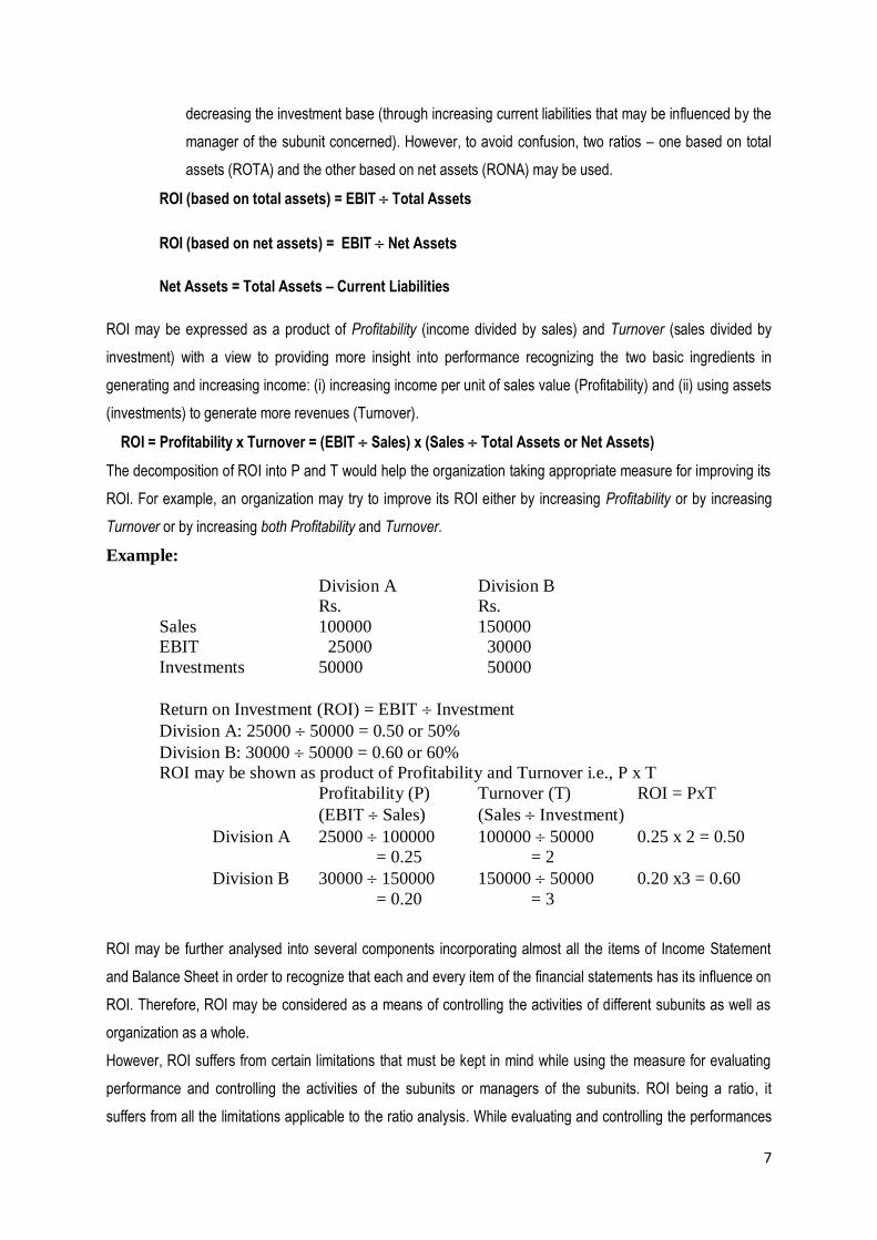
7

decreasing the investment base (through increasing current liabilities that may be influenced by the

manager of the subunit concerned). However, to avoid confusion, two ratios – one based on total

assets (ROTA) and the other based on net assets (RONA) may be used.

ROI (based on total assets) = EBIT Total Assets

ROI (based on net assets) = EBIT Net Assets

Net Assets = Total Assets – Current Liabilities

ROI may be expressed as a product of Profitability (income divided by sales) and Turnover (sales divided by

investment) with a view to providing more insight into performance recognizing the two basic ingredients in

generating and increasing income: (i) increasing income per unit of sales value (Profitability) and (ii) using assets

(investments) to generate more revenues (Turnover).

ROI = Profitability x Turnover = (EBIT Sales) x (Sales Total Assets or Net Assets)

The decomposition of ROI into P and T would help the organization taking appropriate measure for improving its

ROI. For example, an organization may try to improve its ROI either by increasing Profitability or by increasing

Turnover or by increasing both Profitability and Turnover.

Example:

Division A Division B

Rs. Rs.

Sales 100000 150000

EBIT 25000 30000

Investments 50000 50000

Return on Investment (ROI) = EBIT Investment

Division A: 25000 50000 = 0.50 or 50%

Division B: 30000 50000 = 0.60 or 60%

ROI may be shown as product of Profitability and Turnover i.e., P x T

Profitability (P) Turnover (T) ROI = PxT

(EBIT Sales) (Sales Investment)

Division A 25000 100000 100000 50000 0.25 x 2 = 0.50

= 0.25 = 2

Division B 30000 150000 150000 50000 0.20 x3 = 0.60

= 0.20 = 3

ROI may be further analysed into several components incorporating almost all the items of Income Statement

and Balance Sheet in order to recognize that each and every item of the financial statements has its influence on

ROI. Therefore, ROI may be considered as a means of controlling the activities of different subunits as well as

organization as a whole.

However, ROI suffers from certain limitations that must be kept in mind while using the measure for evaluating

performance and controlling the activities of the subunits or managers of the subunits. ROI being a ratio, it

suffers from all the limitations applicable to the ratio analysis. While evaluating and controlling the performances

8

of the divisional managers through ROI, it must be kept in mind that overemphasis on ROI may lead to sub-

optimal decisions. Divisional managers may be tempted to reject the new investment opportunities giving a return

more than the cost of such investments but less than the existing ROI of the division as the acceptance of such

investment project is likely to result in the decrease in ROI. Similarly, there is a possibility that divisional

managers may make an attempt to dispose off any part of the existing investment giving a return less than the

existing ROI, though earning more than the cost of investment, in order to improve its ROI. In both the situations,

the optimum course of action would have been to accept or retain the investment opportunities giving a return

higher than the cost of capital but the action of the divisional managers in order to improve its ROI, as mentioned

above, may result in sub-optimal decisions and consequently, the organization as a whole would be the sufferer.

II. Residual Income (RI) and Economic Value Added (EVA)

RI is the difference between Net Income before Taxes (NIBT) and Capital Charge. Capital Charge is usually

taken as the product of Opening Capital Employed and the Risk-adjusted Cost of Capital (also known as

Required Rate of Return). Therefore, RI may be expressed as follows:

RI = NIBT (or EBIT) – Required Rate of Return x Opening Capital employed.

The move towards the RI measure received even greater publicity when it was renamed into a far more

accessible and acceptable term – Economic Value Added (EVA) – by the Stern Stewart Consulting

organization.

EVA is the difference between the Net Operating Profit after Tax (NOPAT) before interest and the Capital

Charge. To arrive at NOPAT, after-tax but before interest accounting income is required to be adjusted for non-

operating incomes and expenditures, and also for certain adjustments (like Research & Development Expenses,

Employee Training Expenses, Business Re-structuring Expenses, Goodwill, Depreciation, Stock Valuation, etc.)

as suggested by Stern Stewart & Co. Capital Charge for EVA is determined by taking the product of Weighted

Average Cost of Capital (WACC) and Average Capital Employed (Avg. CE). Further, Cost of Equity is derived on

the Capital Asset Pricing Model. EVA may be expressed as follows:

EVA = NOPAT (before Interest on Debt) – WACC x Average Capital Employed …… (i)

= Avg.CE ( NOPAT Avg.CE) – WACC) = Avg. CE (Return on Capital – Cost of Capital) = Avg.CE x Spread ……… (ii)

Differences between RI and EVA

EVA may be considered as refined version of RI, the basic concept behind both the measures being difference

between Income and Capital Charge. However, there are certain differences between these two measures:

(i) RI is calculated on the basis of ‘Before Tax Income’ while EVA is determined on the basis of ‘After Tax Income’;

(ii) n case of RI, ‘Required Rate of Return’ used for calculating ‘Capital Charge’, which may be WACC or may be somewhat different depending on the adjustment for risk factor, but only WACC is considered for EVA.

9

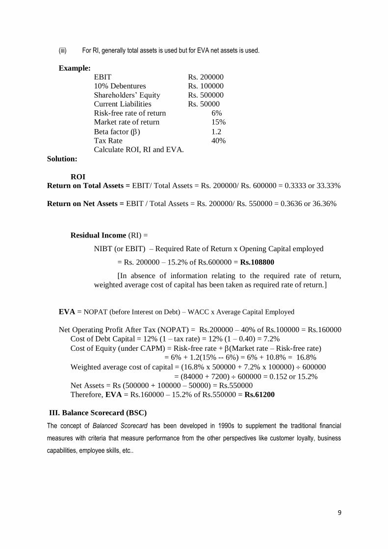
(iii) For RI, generally total assets is used but for EVA net assets is used.

Example:

EBIT Rs. 200000

10% Debentures Rs. 100000

Shareholders’ Equity Rs. 500000

Current Liabilities Rs. 50000

Risk-free rate of return 6%

Market rate of return 15%

Beta factor () 1.2

Tax Rate 40%

Calculate ROI, RI and EVA.

Solution:

ROI

Return on Total Assets = EBIT/ Total Assets = Rs. 200000/ Rs. 600000 = 0.3333 or 33.33%

Return on Net Assets = EBIT / Total Assets = Rs. 200000/ Rs. 550000 = 0.3636 or 36.36%

Residual Income (RI) =

NIBT (or EBIT) – Required Rate of Return x Opening Capital employed

= Rs. 200000 – 15.2% of Rs.600000 = Rs.108800

[In absence of information relating to the required rate of return,

weighted average cost of capital has been taken as required rate of return.]

EVA = NOPAT (before Interest on Debt) – WACC x Average Capital Employed

Net Operating Profit After Tax (NOPAT) = Rs.200000 – 40% of Rs.100000 = Rs.160000

Cost of Debt Capital = 12% (1 – tax rate) = 12% (1 – 0.40) = 7.2%

Cost of Equity (under CAPM) = Risk-free rate + (Market rate – Risk-free rate)

= 6% + 1.2(15% -- 6%) = 6% + 10.8% = 16.8%

Weighted average cost of capital = (16.8% x 500000 + 7.2% x 100000) 600000

= (84000 + 7200) 600000 = 0.152 or 15.2%

Net Assets = Rs (500000 + 100000 – 50000) = Rs.550000

Therefore, EVA = Rs.160000 – 15.2% of Rs.550000 = Rs.61200

III. Balance Scorecard (BSC)

The concept of Balanced Scorecard has been developed in 1990s to supplement the traditional financial

measures with criteria that measure performance from the other perspectives like customer loyalty, business

capabilities, employee skills, etc..

10

Balanced Scorecard help measure how the business units create value for current and future customers, how

they must develop and increase internal capabilities, and the investment in people, system, and procedures

necessary to improve future performance. The Balanced Scorecard incorporates both financial and non-financial

perspectives into its fold and captures the critical value creating activities. Hence, a properly constructed

Balanced Scorecard may be used in measuring total business unit performance.

The BSC was developed to communicate the multiple, linked objectives that companies must achieve to

compete on the basis of capabilities and innovation, not just tangible physical assets. The BSC translates

mission and strategy into objectives and measures, organized into four perspectives:

Financial

Customer

Internal Business Process and

Learning and Growth

Financial measures in the Financial Perspective of the BSC indicate whether the company’s strategy,

implementation, and execution are contributing to bottom-line improvement.

In the Customer Perspective, the customer and market segment in which the business unit competes, and the

business unit’s performance in the targeted segments are identified.

In the Internal Business Process Perspective, executives identify the critical internal processes in which the

organization must excel in order to deliver the value propositions that will attract and retain customers in targeted

market segments and satisfy shareholder expectations of excellent financial returns.

The fourth perspective, Learning and Growth, identifies the infrastructure that the organization must build to

create long-term growth and improvement.

BSC is not only a comprehensive performance measurement system but it may also be used as the foundation

of a strategic management system. In the words of Kaplan and Norton, ‘companies are using the scorecard to

Clarify and update strategy,

Communicate strategy throughout the company,

Align unit and individual goals with the strategy,

Link strategic objectives to long-term targets and annual budgets,

Identify and align strategic initiatives, and

Conduct periodic performance reviews to learn about and improve strategy.

D.R.Dandapat, Dept of Commerce, CU Suggested Readings:

Banerjee, B., Cost Accounting, PHI, New Delhi

Banerjee, B., Financial Policy and Management Accounting, PHI, New Delhi

Drury, C., Management and Cost Accounting, Chapman & Hall, London,/ Thomson Learning

Horngren, Foster and Datar, Cost Accounting – A Managerial Emphasis, PHI, New Delhi

Hilton, R.W., Managerial Accounting, Tata McGraw-Hill, New Delhi

Kaplan, R.S., and Atkinson, A.A., Advanced Management Accounting, PHI, New Delhi

11

1

Paper CC 402: Strategic Cost and ManagementAccounting (SCM)

Module –I

Transfer Pricing

(Prof. Ashish Kumar Sana)

A transfer price is the amount charged when one division of an organization sells

goods or services to another division.

Transfer pricing is the determination of an exchange price for a product or service

when different business units within a firm exchange it. The products can be final

products sold to customers or intermediate products. This determination of transfer

price is desirable from both a management perspective and tax purposes. Transfer of

goods and services between business units is most common in firms with a high

degree of vertical integration. Vertically integrated firms engage in a number of

different value-creating activities in the value chain (Blocher, Chen, Cokins and Lin,

2006).

Objectives of Transfer Pricing

i) To motivate managers

ii) To provide an appropriate incentive for managers to make decisions consistent

with the firm’s goals

iii) To provide a basis for fairly rewarding the managers

iv) To develop strategic partnerships.

A relatively high transfer price might also be used to encourage internal units to

purchase from an external supplier, to encourage an external business relationship the

firm wants to develop because of the supplier’s quality, or to gain entrance to a market

in a new country (Blocher, Chen, Cokins and Lin, 2006).

2

International Transfer Pricing Objectives Minimiation of customs charges Currency restrictions Risk of Expropriation

Source: Hilton Ronad W., (2005), Managerial Accounting, Tata McGraw Hill, P557

3

Transfer Pricing Methods

Transfer Pricing Decisions

1. When the supplying division has excess capacity, the range of transfer price would be

(a) Minimum Transfer Price= Marginal Cost per Unit

(b) Maximum Transfer Price=Lower of Net Marginal Revenue and the External Buy-in-

Price

2. When the supplying division operates at full capacity, the range of transfer price would be

(a) Minimum Transfer Price= Marginal Cost per Unit + Opportunity Cost per Unit

(b) Maximum Transfer Price=Lower of Net Marginal Revenue and the External Buy-in-

Price

Cost basedMethod

Marginal Cost Standard Cost

3

Transfer Pricing Methods

Transfer Pricing Decisions

1. When the supplying division has excess capacity, the range of transfer price would be

(a) Minimum Transfer Price= Marginal Cost per Unit

(b) Maximum Transfer Price=Lower of Net Marginal Revenue and the External Buy-in-

Price

2. When the supplying division operates at full capacity, the range of transfer price would be

(a) Minimum Transfer Price= Marginal Cost per Unit + Opportunity Cost per Unit

(b) Maximum Transfer Price=Lower of Net Marginal Revenue and the External Buy-in-

Price

TransferPricing

Methods

Standard Cost Full Cost Cost PlusMarkup

Market BasedMethod

NegotiatedBased Method

3

Transfer Pricing Methods

Transfer Pricing Decisions

1. When the supplying division has excess capacity, the range of transfer price would be

(a) Minimum Transfer Price= Marginal Cost per Unit

(b) Maximum Transfer Price=Lower of Net Marginal Revenue and the External Buy-in-

Price

2. When the supplying division operates at full capacity, the range of transfer price would be

(a) Minimum Transfer Price= Marginal Cost per Unit + Opportunity Cost per Unit

(b) Maximum Transfer Price=Lower of Net Marginal Revenue and the External Buy-in-

Price

Cost PlusMarkup

NegotiatedBased Method

4

Example:

Division X is a profit centre, which produces four products P, Q, R, S. Each product is sold in

the external market also. Following information is available for the period:

Particulars P Q R S

Market price p.u. (Rs.) 700 690 560 460

Variable Cost p.u. (Rs.) 660 620 360 370

Labour hours required p.u. 3 4 2 3

Product S can be transferred to Division Y but the maximum quantity that might required for

transfer is 2000 units of S.

The maximum sales in the external market are:

P 3000 Units

Q 3500 Units

R 2800 Units

S 1800 Units

Division Y can purchase the same product at a slightly cheaper price of Rs.450 p.u. instead of

receiving transfers of product S from Division X.

What should be the transfer price for each unit for 2000 units of S, if the total labour hours

available in Division X are: (i) 24,000 hours and (ii) 32,000 hours?

Solution:

Calculation of Ranking of Products when availability of time is the key factor

No Particulars P Q R S

1 Market price p.u. (Rs.) 700 690 560 460

2 Less: Variable Cost p.u. (Rs.) 660 620 360 370

3 Contribution p.u. (1-2) 40 70 200 90

4 Labour hours required p.u. 3 4 2 3

5 Contribution per hour (3÷4) 13.33 17.50 100 30

6 Ranking IV III I II

5

Situation 1 : When labour hours available in Division X is 24, 000 hours

Statement showing product mix

Product

(Ranking)

Maximum Demand

(Units)

Hours

p.u.

Units

Produced

Hours

Used

Balance Hours

R 2800 2 2800 5600 (24000-5600)=18400

R 1800 3 1800 5400 (18400-5400)=13000

Q 3500 4 3250 13000 (13000-13000)=0

P 3000 3 0 0 0

Statement showing Transfer Price for each unit for 2000 units of Product S

Transfer Price 2000 units of product S(Rs.)

Per unit of Product S(Rs.)

Variable Cost (Rs.) 7,40,000 370Opportunity Cost of theContribution foregone by notproducing 1,500 units of Q(1500 units ×Rs.70)

1,05,000 52.50

Transfer price 8,45,000 422.50

Note: Time required to meet the demand of 2,000 units of Product S for Division Y is 6000

hours. This requirement of time viz. 6,000 hours for providing 2,000 units of Product S for

Division Y can be met by sacrificing the production of 1,500 units of Product Q

(1500 units ×4 hours).

Situation 2 : When labour hours available in Division X is 32, 000 hours

Statement showing product mix

Product

(Ranking)

Maximum Demand

(Units)

Hours

p.u.

Units

Produced

Hours

Used

Balance Hours

R 2800 2 2800 5600 (32000-5600)=26400

R 1800 3 1800 5400 (26400-5400)=21000

Q 3500 4 3500 13000 (21000-14000)=7000

P 3000 3 2333 0 (7000-7000)=0

6

Statement showing Transfer Price for each unit for 2000 units of Product S

Transfer Price 2000 units of product S(Rs.)

Per unit of Product S(Rs.)

Variable Cost (Rs.) 7,40,000 370Opportunity Cost of theContribution foregone by notproducing 2,000 units of P (2000units ×Rs.40)

80,000 40.00

Transfer price 8,20,000 410.00

Note: Time required to meet the demand of 2,000 units of Product S for Division Y is 6000

hours. This requirement of time viz. 6,000 hours for providing 2,000 units of Product S for

Division Y can be met by sacrificing the production of 2,000 units of Product P

(2000 units ×3 hours).

7

Unit 7: Responsibility Accounting and Reporting

Responsibility Accounting:

“Responsibility accounting collects and reports planned and actual accounting information

about the inputs and outputs of responsibility centres” (Anthony and Welsch, 1977). So, it is

a device to measure divisional performance of an organisation.

(Source: https://www.wallstreetmojo.com/responsibility-accounting/)

Features of Responsibility Accounting:

i) Inputs and Outputs: Responsibility accounting is based on cost (inputs) and revenues

(outputs) data for financial information.

ii) Planned and Actual: For financial planning and control of an organisation, it is not only

contains historical information about costs and revenues, but also estimated future cost

and revenue data.

iii) Responsibility Centres: Responsibility accounting focuses on responsibility centres.

Responsibility Centre is a unit or sub-unit of an organization. There is a manager for each

centre who is responsible for each centre.

Types of Responsibility Centre:

8

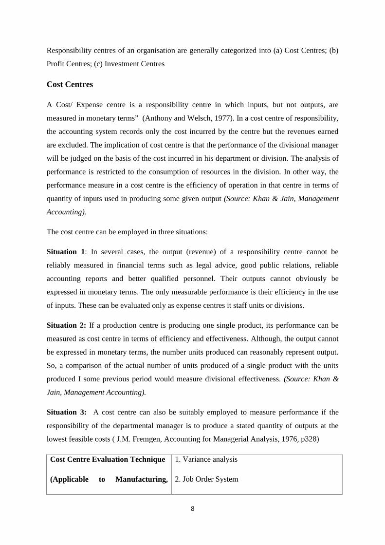
Responsibility centres of an organisation are generally categorized into (a) Cost Centres; (b)

Profit Centres; (c) Investment Centres

Cost Centres

A Cost/ Expense centre is a responsibility centre in which inputs, but not outputs, are

measured in monetary terms” (Anthony and Welsch, 1977). In a cost centre of responsibility,

the accounting system records only the cost incurred by the centre but the revenues earned

are excluded. The implication of cost centre is that the performance of the divisional manager

will be judged on the basis of the cost incurred in his department or division. The analysis of

performance is restricted to the consumption of resources in the division. In other way, the

performance measure in a cost centre is the efficiency of operation in that centre in terms of

quantity of inputs used in producing some given output (Source: Khan & Jain, Management

Accounting).

The cost centre can be employed in three situations:

Situation 1: In several cases, the output (revenue) of a responsibility centre cannot be

reliably measured in financial terms such as legal advice, good public relations, reliable

accounting reports and better qualified personnel. Their outputs cannot obviously be

expressed in monetary terms. The only measurable performance is their efficiency in the use

of inputs. These can be evaluated only as expense centres it staff units or divisions.

Situation 2: If a production centre is producing one single product, its performance can be

measured as cost centre in terms of efficiency and effectiveness. Although, the output cannot

be expressed in monetary terms, the number units produced can reasonably represent output.

So, a comparison of the actual number of units produced of a single product with the units

produced I some previous period would measure divisional effectiveness. (Source: Khan &

Jain, Management Accounting).

Situation 3: A cost centre can also be suitably employed to measure performance if the

responsibility of the departmental manager is to produce a stated quantity of outputs at the

lowest feasible costs ( J.M. Fremgen, Accounting for Managerial Analysis, 1976, p328)

Cost Centre Evaluation Technique

(Applicable to Manufacturing,

1. Variance analysis

2. Job Order System

9

product-line, marketing, function

or other segments)

3. Processing Costing System

Profit Centres:

A profit centre is a responsibility centre in which inputs are measured in terms of expenses

and outputs are measured in terms of revenues ” (Anthony and Welsch, 1977, Management

Accounting). Both costs and revenues of the centre are accounted for in this centre. Profit

analysis can be used as a basis for evaluating the performance of a divisional manager.

Management can determine whether the division was effective in attaining its objectives or

not. This objective is presumably to earn a “satisfactory profit”. The performance of the

managers is measured by profit. In other words, managers can be expected to behave as if

they were running their own business. For this reason, the profit centre is good training for

general management responsibility.

As a measurement of performance, profit centre can be used (i) for evaluation and ranking of

profit centres (ii) as a basis for decisions to modify operations of profit centres.

Investment Centres:

A investment centre is a responsibility centre in which inputs are measured in terms of

costs/expenses and outputs are measured in terms of revenues in which assets employed are

also measured ” (Anthony and Welsch, 1977, Management Accounting).

Investment centres consider not only cost and revenues but also the assets used in the

division. As a responsibility centre, the performance of a unit would be measured in relation

to the revenues/profits and the assets employed in a division. The measure of performance in

an investment centre is based on the relationship between the segment profit contribution and

segment assets. There are two ways to relate segment profit contribution to segment

resources: (i) Segment Rate of Return on Investment (SROI)

(ii) Segment Residual Income

10

Segment Rate of Return on Investment (SROI)

(1) Segment Rate of Return on Investment (SROI) = ( )/ ( / ) × 100(2) Segment Rate of Return on Investment (SROI) =

×(3) SROI (Operating ) =

× 100(4) SROI (Net) =

× 100Segment Residual Income (SRI) = SPC-(SROI×SR)

Suggested Readings:

Khan and Jain, Management Accounting, The McGraw-Hill

Blocher, Chen, Cokins and Lin, Cost Management-A Strategic Emphasis, The TataMcGraw-Hill

Hilton, Managerial Accounting, The Tata McGraw-Hill

Study Materials of The Institute of Chartered Accountants of India

Study Materials of The Institute of Cost Accountants of India

Page | 1

Department of Commerce

University of Calcutta

Study Material

Cum

Lecture Notes

Only for the Students of M.Com. (Semester IV)-2020

University of Calcutta

(Internal Circulation)

Page | 2

Dear Students, Hope you, your parents and other family members are safe and secured. We are going

through a world-wide crisis that seriously affects not only the normal life and economy

but also the teaching-learning process of our University and our department is not an

exception.

As the lock-down is continuing and it is not possible to reach you physically. Keeping in

mind the present situation, our esteemed teachers are trying their level best to reach

you through providing study material cum lecture notes of different subjects. This

material is not an exhaustive one though it is an indicative so that you can understand

different topics of different subjects. We believe that it is not the alternative of direct

teaching learning.

It is a gentle request you to circulate this material only to your friends those who are

studying in Semester IV (2020).

Stay safe and stay home.

Best wishes.

Page | 3

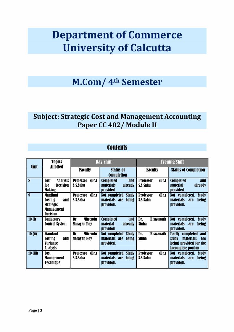
Department of Commerce University of Calcutta

M.Com/ 4th Semester

Subject: Strategic Cost and Management Accounting Paper CC 402/ Module II

Contents

Unit

Topics

Allotted Day Shift Evening Shift

Faculty Status of

Completion

Faculty Status of Completion

8 Cost Analysis

for Decision

Making

Professor (Dr.)

S.S.Saha

Completed and

materials already

provided

Professor (Dr.)

S.S.Saha

Completed and

material already

provided

9 Marginal

Costing and

Strategic

Management

Decision

Professor (Dr.)

S.S.Saha

Not completed. Study

materials are being

provided.

Professor (Dr.)

S.S.Saha

Not completed. Study

materials are being

provided.

10 (i) Budgetary

Control System

Dr. Mitrendu

Narayan Roy

Completed and

material already

provided

Dr. Biswanath

Sinha

Not completed. Study

materials are being

provided.

10 (ii) Standard

Costing and

Variance

Analysis

Dr. Mitrendu

Narayan Roy

Not completed. Study

materials are being

provided.

Dr. Biswanath

Sinha

Partly completed and

study materials are

being provided for the

incomplete portion

10 (iii) Cost

Management

Technique

Professor (Dr.)

S.S.Saha

Not completed. Study

materials are being

provided.

Professor (Dr.)

S.S.Saha

Not completed. Study

materials are being

provided.

Page | 4

Name of the Faculty: Professor (Dr.) S.S.Saha

[ DAY AND EVENING SHIFT ]

TOPICS

• Unit 8: Cost Analysis for Decision Making

• Unit 9: Marginal Costing and Strategic Management

Decision

• Unit 10(iii): Cost Management Technique

Unit 8: Cost Analysis for Decision Making Matters related to this topic were already discussed in details in the classes and appropriate materials were provided to the students.

Unit 9: Marginal Costing and Strategic Management Decision

Contents: Marginal cost and strategic management decisions —consideration of limiting factor in decision making— make or buy, adding or dropping a product line, shutdown or continue, special order/ export order, product-mix, pricing decisions

Page | 5

Marginal cost and Strategic Management Decision Marginal costing is based on the principle of dividing all costs into fixed cost and variable cost. Fixed costs are unrelated to the levels of production. These costs remain the same irrespective of the production quantities. Variable costs change in relation to production levels. They are directly proportionate. The variable cost per unit, however, remains the same. In marginal costing, these variable costs are only considered while calculating the production costs. Of all the available techniques of costing, marginal costing is most suitable for making decisions like how much material to buy, the correct product mix, fixing the selling price, etc. Decision making is a very important factor in every firm. Decision making means choosing or selecting a course of action from a given set of alternatives. Application of marginal costing plays a very significant role in this regard particularly for managerial decisions. These are as follows:

• Make or buy decision; • Adding or dropping a product line; • Shut-Down or Continue decision; • Accepting additional orders and exploring foreign market; • Selection of most profitable mix; and • Fixation of selling price;

Consideration of Limiting Factor/ Key Factor

Limiting Factor which limits production and/ or sales comprises shortage of materials,

labour, plant capacity, sales demand, etc. In case of decision making with regard to

selection of profitable product –mix, optimum sales-mix, make or buy, appropriate

criteria in relation to limiting factor should be taken into consideration.

MAKE OR BUY DECISION A manufacturing concern may sometimes have to take the decision whether to buy a component or services required for final production or whether to make it in-house. However, make or buy decision under different situations can be made as follows:

CASE-I: When Company having spare/ unused capacity in making components parts instead of buying them from market.

(i) When Manufacture involves only variable costs assuming that fixed costs were

already incurred and fixed costs are not relevant, whether one should make or buy :

If Variable Cost / Marginal Cost < Purchase Price, it is advisable to

make/manufacture the components parts in the factory.

Illustration-1 X Manufacturing Company having unused capacity requires component-A 20000 units @ Rs. 60 per unit to manufacture a final product. Total manufacturing costs of Rs. 64 per unit comprise Rs. 32 as raw material, Rs. 12 as direct labour, Rs. 6 as variable overhead,

Page | 6

Rs. 6 as avoidable fixed overhead, and Rs. 8 as other fixed overhead allocated on the basis of capacity utilized. Required

(i) Should the company make or buy the component-A? (ii) Determine the range of production at which one is more profitable than the other.

Solution

(i) Should the company make or buy the component-A? Purchase price of component-A = Rs. 60 Manufacturing costs per unit of component-A (Relevant Cost= Variable Cost /

Marginal Costs + Avoidable fixed costs )= (Rs. 32 as raw material + Rs. 12 as direct labour +Rs. 6 as variable overhead) + Rs. 6 as avoidable fixed overhead = Rs.56

Decision: The company should make the component-A as Manufacturing costs< Purchase price

(ii) Determine the range of production at which one is more profitable than the

other Minimum Volume of Production (at which both the alternatives making and buying

are equally profitable) which will justify ‘Making’ as compared to ‘Buying’ Minimum Volume of Production = Increase in fixed costs ÷ Contribution Per Unit =

Rs. 120000÷ Rs.10= 12000 units Increase in fixed costs = Rs. 6 as avoidable fixed overhead × 20000 units = Rs.

120000 Contribution Per Unit = Purchase Price – Variable/ Marginal Cost (excluding

Avoidable FCs) = Rs. 60 – Rs. 50 = Rs.10

Decision: (a) From 1 to 11999 units, buying will be more profitable and (b) from 12001 units to 20000 units, making will be more profitable

CASE-II: When Company does not have spare/ unused capacity in making the components parts.

(i) When Manufacture involves increase in fixed costs (Avoidable fixed costs) and fixed costs are relevant here as relevant cost/ product cost, whether one should make or buy: If Relevant Cost (Variable/ Marginal Cost + Avoidable fixed costs) < Purchase

Price, it is advisable to make/manufacture the components parts in the factory.

One can determine the Minimum Volume of Production (at which both the alternatives making and buying are equally profitable) which will justify ‘Making’ as compared to ‘Buying’.

Minimum Volume of Production = [Increase in fixed costs ÷ Contribution Per Unit]

Contribution Per Unit = [purchase price – Variable/ Marginal Cost (excluding

Avoidable fixed costs)]

Page | 7

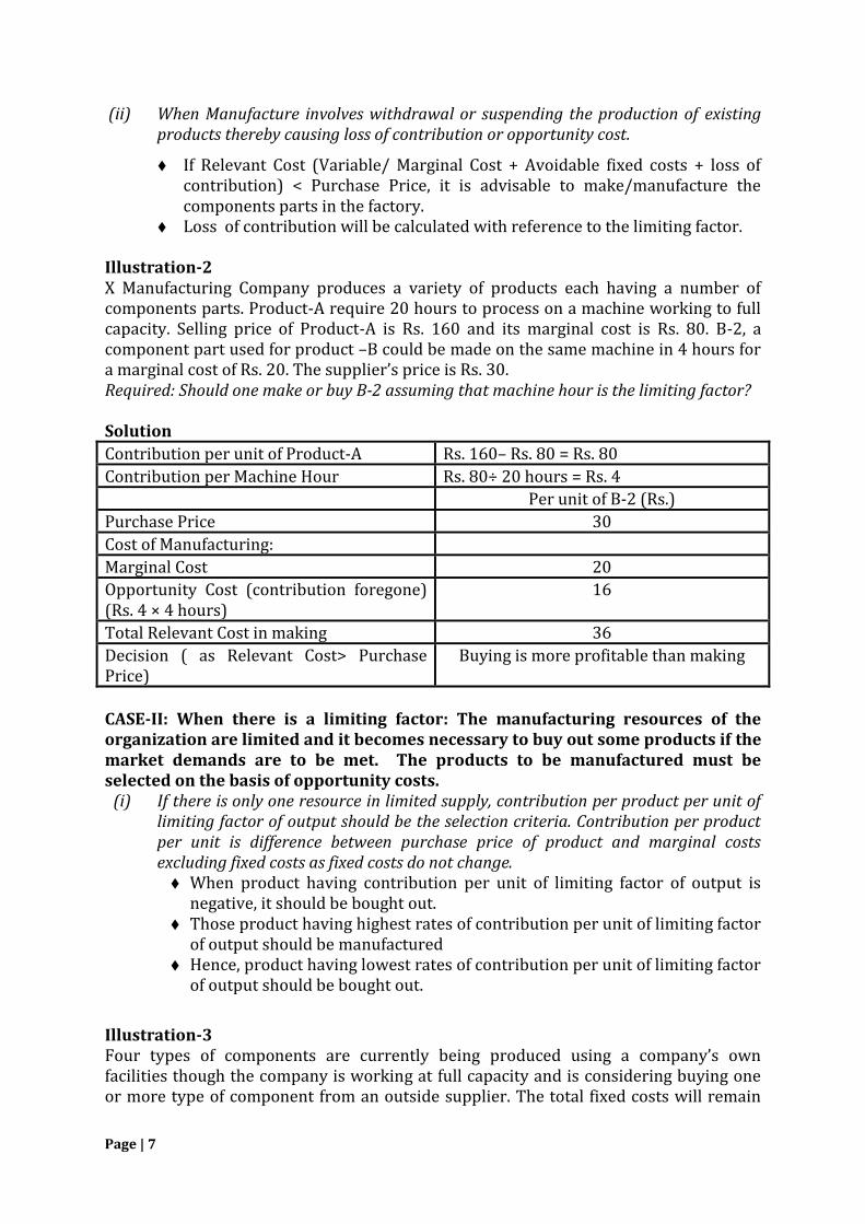
(ii) When Manufacture involves withdrawal or suspending the production of existing products thereby causing loss of contribution or opportunity cost.

If Relevant Cost (Variable/ Marginal Cost + Avoidable fixed costs + loss of contribution) < Purchase Price, it is advisable to make/manufacture the components parts in the factory.

Loss of contribution will be calculated with reference to the limiting factor.

Illustration-2 X Manufacturing Company produces a variety of products each having a number of components parts. Product-A require 20 hours to process on a machine working to full capacity. Selling price of Product-A is Rs. 160 and its marginal cost is Rs. 80. B-2, a component part used for product –B could be made on the same machine in 4 hours for a marginal cost of Rs. 20. The supplier’s price is Rs. 30. Required: Should one make or buy B-2 assuming that machine hour is the limiting factor? Solution

Contribution per unit of Product-A Rs. 160– Rs. 80 = Rs. 80

Contribution per Machine Hour Rs. 80÷ 20 hours = Rs. 4

Per unit of B-2 (Rs.)

Purchase Price 30

Cost of Manufacturing:

Marginal Cost 20

Opportunity Cost (contribution foregone) (Rs. 4 × 4 hours)

16

Total Relevant Cost in making 36

Decision ( as Relevant Cost> Purchase Price)

Buying is more profitable than making

CASE-II: When there is a limiting factor: The manufacturing resources of the organization are limited and it becomes necessary to buy out some products if the market demands are to be met. The products to be manufactured must be selected on the basis of opportunity costs.

(i) If there is only one resource in limited supply, contribution per product per unit of limiting factor of output should be the selection criteria. Contribution per product per unit is difference between purchase price of product and marginal costs excluding fixed costs as fixed costs do not change. When product having contribution per unit of limiting factor of output is

negative, it should be bought out. Those product having highest rates of contribution per unit of limiting factor

of output should be manufactured Hence, product having lowest rates of contribution per unit of limiting factor

of output should be bought out.

Illustration-3 Four types of components are currently being produced using a company’s own facilities though the company is working at full capacity and is considering buying one or more type of component from an outside supplier. The total fixed costs will remain

Page | 8

unaffected for the company as a whole with the making in or buying out of the component. From the following information, which component or components would you recommend to be bought out when (a) labour time is the limiting factor; (b) machine time is the limiting factor?

Components A B C D

Time per unit:

Labour Hours 0.40 0.50 0.50 0.30

Machine Hours 0.10 0.20 0.40 0.50

Cost per unit: (Rs.) (Rs.) (Rs.) (Rs.)

Marginal costs (Rs.) 10 12 15 15

Fixed costs (allocated) 2 4 5 15

Total costs 12 16 20 30

Purchase price 9 17 22 24

Solution

A(Rs.) B(Rs.) C(Rs.) D(Rs.)

Purchase price 9 17 22 24

Less: Marginal costs (Rs.)

10 12 15 15

Contribution per unit (–) 1 5 7 9

Contribution per Labour Hour

(–) 2.5 10 14 30

Contribution per Machine Hour

(–) 10 25 17.5 18

Should be bought out

Decision:

When Labour Hour is limiting factor, order of selection for buying based on lowest rates of contribution per unit of limiting factor would be : B,C,D

When Machine Hour is limiting factor, order of selection for buying based on lowest rates of contribution per unit of limiting factor would be : C,D ,B

Illustration-4 A Ltd. manufactures and sells 25000 units of product annually. One of the components required for production is procured from outside supplier at Rs. 190/ unit. Annually it is purchasing 25000 units for its usage. If the component is produced in the own plant, annual production can be increased by 5000 units. Costs of the components are as follows:

Rs./ unit Direct material 80 Direct labor 75 Factory overhead (70% variable) 40 Total cost 195

Page | 9

If the component is made in-house, in order to market the additional units, overall price should be reduced by 5% and additionally Rs. 100000 p.m. should be incurred for advertising. Present selling price and contribution of the product are Rs. 2500/ unit and Rs. 600 respectively. Analyze the make or buy decision on unit basis and total basis and recommend the profitable alternative. Solution: Variable cost of producing the component:

Rs./ unit Direct material 80 Direct labor 75 Factory overhead (70% variable) 28 Total variable cost 183

If A Ltd. decides to manufacture the component in-house, the capacity would

increase from 25000 to 30000. Since 25000 components are purchased to produce 25000 units, component usage is

1 component/ unit. Variable cost of the product will be [(2500 – 600) – 190] = Rs. 1710/ unit. Fixed overhead of Rs. 12/ unit will be incurred irrespective of the fact that the

component is manufactured or not. Increase in advertising expenses would be Rs. 1200000 (Rs. 100000 × 12) Overall selling price would reduce from Rs. 2500 to Rs. 2375 (Rs. 2500 x 95%) Current contribution considering the procurement price of Rs. 190 for the

component is Rs. 600. Since, variable cost of procurement is Rs. 183, in case of in-house manufacture; contribution would increase by Rs. 7 (Rs. 190 – Rs. 183). On the other hand, selling price is getting reduced by Rs. 125 (Rs. 2500 x 5%). Hence, contribution in case of make decision is (Rs. 600 + Rs. 7 – Rs. 125) = Rs. 482.

It can be summarized as follows: Particulars Procurement of 25000 components Produce 30000 components Per unit (Rs.) Total (Rs.) Per unit (Rs.) Total (Rs.) Selling price 2500 62500000 2375 71250000 Contribution 600 15000000 482 14460000

Incremental loss in contribution is Rs. 540000 (Rs. 15000000 – Rs. 14460000). Overall incremental loss is Rs. 1740000 (Rs. 540000 + Rs. 1200000 for advertising) which is Rs. 68/ unit.

In this particular situation, A Ltd. should go for buy decision.

SHUT-DOWN OR CONTINUE DECISION/ ADDING OR DROPPING A PRODUCT LINE Decisions are taken for closure of a particular segment (division, product line, services, departments, stores, or outlets) based on incremental revenue lost and incremental cost savings generated out of such decision.

• Incremental revenue lost = Original revenue – Revenue after dropping the segment. Revenue generated due to increase in demand for other segments that should be considered in incremental revenue.

Page | 10

• Incremental cost savings involve variable costs and specific avoidable fixed costs associated with the segment.

• If the segment can be used for any other purpose (lease/ rent) the incremental opportunity costs should also be considered.

• If incremental cost savings > incremental revenue lost, the segment should be discontinued and vice versa. However, if they are equal, then decisions are taken based on qualitative factors, such as impact on employees of that segment, impact on suppliers and customers, etc.

Illustration-5

R Ltd. is contemplating shutting down its Division C. The following information is given: Particulars A & B C Total Maximum achievable sales (Rs.) 4140000 517500 4657500 Less: variable cost (Rs.) 2070000 276000 2346000 Contribution (Rs.) 2070000 241500 2311500 Less: Specific avoidable fixed cost (Rs.) 1449000 414000 1863000 Divisional income (Rs.) 621000 (172500) 448500 The rates of variable cost are 90% of the normal rates due to current volume of operation. However, if the current volume goes down, the rate will go back to normal. Comment on shutting down division C. Solution: Incremental loss/ savings due to discontinuance of division C Particulars Nature Rs. Specific avoidable fixed cost Savings due to discontinuation 414000 Contribution Loss due to discontinuation (241500) Variable cost (2070000 x 10/90)

Increase in variable cost due to discontinuation

(230000)

Savings/ (loss) due to discontinuation (57500) Since there is a loss due to discontinuation, C should not be discontinued.

ACCEPTING ADDITIONAL ORDERS AND EXPLORING FOREIGN MARKET (SPECIAL ORDER/

EXPORT ORDER) DECISION If the manufacturing concern is working below its productive capacity, special orders or export orders may be attractive to them. In such orders, the concern is asked to deliver certain quantities of the product at a special price which would result in incremental revenue for the concern. However, accepting such offer would also require the concern to incur certain incremental variable costs (special packing, commission, shipping, etc.) and incremental fixed cost (inspection).

• If the incremental revenue > incremental cost, the special order should be accepted and vice versa.

Page | 11

• If the concern is working at its full capacity, in order to accept the order, it may have to forego the orders from its existing customers. Management has to qualitatively evaluate whether that would be a prudent decision.

Illustration-6 B Ltd. is engaged in the manufacture of product X by joint process of 5 machines. Machines are capable of producing 40 units of X/ hour. The variable cost/ unit is Re. 0.32 and selling price/ unit is Re. 0.80. B Ltd. received an order from another company to manufacture 40000 units of Y, a separate product the price of which is Rs. 30/ unit and variable cost is Rs. 24/ unit. The additional cost to be incurred to take up this order is Rs. 100000. The existing machines can produce 16 units of Y/ hour. The company has a total capacity of 10000 hours during the period in which the toy is required to be manufactured. The fixed cost excluding the aforementioned additional cost is Rs. 1000000. The company has an existing order for supply of 400000 X during the period. Do you advise the company to take up this special order? Solution: Statement showing contribution/ machine hour Particulars X Y Demand (units) 300000 40000 Sales (Rs./ unit) 0.80 30 Less: Variable cost (Rs./ unit) 0.32 24 Less: Specific fixed cost (Rs./ unit) 2.50 Contribution 0.48 3.50 Machine hour required/ unit 0.025 0.0625 Contribution/ machine hour 19.20 56.00 Since, contribution/ machine hour for product Y is higher, B Ltd. may provide priority to the special order. Total machine hour required for Y is 2500 hours. Hence, remaining 7500 hours can be utilized for producing X. However, with the remaining machine hours only 300000 units can be produced. B Ltd. may have to take decision whether it should go for the special order for better contribution or stick to the existing order of 400000 units of X to build better customer relationship.

MOST PROFITABLE MIX DECISION Decisions are often taken whether to produce one product in place of another or what should be optimum combination of the products. This is decided based on contribution/ unit of the products concerned. If the concern has limited resource for a key factor (e.g. machine hour), per unit contribution for one unit of the limiting factor is to be calculated. The product with higher contribution should be produced. Illustration-7 P Ltd. produces two products – X and Y. The cost information of these two products is presented as follows: Particulars X Y

Page | 12

Direct material (Rs./ unit) 10 9 Direct wages (Rs./ unit) 3 2 Selling price (Rs./ unit) 20 15 The fixed cost is Rs. 800. Variable cost is allotted to products as 100% of direct wages. Sales mixtures: 100 units of product A and 200 units of product Y 150 units of product X and Y 200 units of product X and 100 units of product Y You are suggested to recommend which sales-mixture to be adopted. Solution: Calculation of contribution

(Rs./ unit) Particulars X Y Selling price 20 15 Less: Direct Materials 10 9 Less: Direct wages 3 2 Less: Variable overhead 3 2 Contribution 4 2 PV ratio 20% 13.5% Identification of optimum product mix Products Contribution/

unit Plan A Plan B Plan C

Units Value Units Value Units Value X 4 100 400 150 600 200 800 Y 2 200 400 150 300 100 200 Total 300 800 300 900 300 1000 Since, total contribution is highest under Plan C, it should be adopted. Illustration-8 An agro-products procedure company is planning its production for the next year. The

following information is relating to the current year:

Products /Crops X1 X2 Y1 Y2 Area Occupied (acres) 250 200 300 250 Yield per acre (ton) 50 40 45 60 Selling price per ton (Rs.) 200 250 300 270 Variable cost per acre(Rs.): Seeds 300 250 450 400

Pesticides 150 200 300 250

Fertilizers 125 75 100 125

Cultivations 125 75 100 125

Direct Wages 4000 4500 5000 5700

Page | 13

Fixed overhead per annum is Rs. 53, 76,000. The land that is being used for the

production of Y1 and Y2 can be used for either crop, but not for X1 and X2 . The land that

is being used for the production of X1 and X2 can be used for either crop, but not for Y1

and Y2 . In order to provide an adequate market service, the company must produce

each year at least 2000 tons each of X1 and X2 and 1800 tons each of Y1 and Y2. You are

suggested to

(i) prepare a statement of the profit for the current year; (ii) prepare a statement of the profit for the production mix by fulfilling market

commitment. Solution: (i) Statement showing the profit for the current year

Products /Crops X1 X2 Y1 Y2 Total

A Yield per acre (ton)

50 40 45 60

B Selling price per tones (Rs.)

200 250 300 270

C Sales revenue per acre(Rs.) [A× B]

10000 1000 13500 16200

D Variable cost per acre(Rs.)

4700 5100 5950 6600

E Contribution per acre(Rs.) [C― D]

5300 4900 7550 9600

F Area (acres) 250 200 300 250

G Total Contribution (Rs.) [E× F]

13,25,000 9,80,000 22,65,000 24,00,000 69,70,000

Less: Fixed Cost(Rs.)

--- --- --- --- 53, 76,000

Profit (Rs.) 15,94,000

(ii) Statement showing profit for the Recommended Mix

Products /Crops X1 X2 Y1 Y2 Total

Contribution per acre(Rs.)

5300

4900 7550 9600

Rank 1 2 2 1

Minimum Tones 2000 2000 1800 1800

Acres required 40 [ 2000÷50]

50 [ 2000÷40]

40[1800÷45] 30 [1800÷60]

Balance acres 360 --- --- 480

Recommended Mix in acre

400 50 40 510

Total Contribution (Rs.)

21,20,000 2,45,000 3,02,000 48,96,000 75, 63,000

Less: Fixed Cost(Rs.) --- --- --- --- 53, 76,000

Page | 14

Profit (Rs.) 21,87,000

FIXATION OF SELLING PRICE DECISION The lowest price at which a concern may sell its product is determined based on relevant cost of manufacturing (incremental cost + opportunity cost if any). Pricing decision is important in case of intense competition, surplus production capacity, clearance of old inventories, getting special orders and improving market share. Illustration-9 L Ltd. wants increase their volume of sales by 100% while maintaining present level of profit. Any change in fixed or variable costs are not anticipated. The following information is obtained from their books:

Sales of 70000 units Rs. 840000 Variable cost Rs. 5/ unit Fixed cost Rs. 50000

At what price they should be ready to sell their product? Solution: Statement showing current profit Sales Rs. 840000 Variable costs (70000 × Rs. 5) Rs. 350000 Contribution Rs. 490000 Fixed cost Rs. 50000 Profit Rs. 440000 Current PV ratio: Rs. 490000÷ Rs. 840000 = 58.33%. Present selling price/ unit = Rs. 840000÷70000 = Rs. 12 Present contribution/ unit = Rs. 490000÷ 70000 = Rs. 7 Since the company wants to increase their volume of sales by 100%, new sales quantity = 70000 × 2 = 140000 units. (Fixed cost + desired profit)/ Future PV ratio = Future sales Or, (Rs. 50000 + Rs. 440000) = Future sales × Future PV ratio Or, Future contribution = Rs. 490000 Or, (Future selling price/ unit ― Rs. 5) × 140000 = Rs. 490000 Or, Future selling price/ unit = Rs. 8.5 So, in order to increase volume of sales by 100%, L Ltd. should set the selling price at Rs. 8.5/unit.

Page | 15

Unit 10(iii): Cost Management Technique Contents: Cost control and cost reduction, benchmarking, value chain analysis and value engineering/value analysis

Cost Control and Cost Reduction Cost Control is a process in which a focus is made on controlling the total cost through competitive analysis. It is a practice which works to align the actual cost in agreement with the established norms. It ensures that the cost incurred on production should not go beyond the pre-determined cost. Cost Control involves a chain of various activities, which starts with the preparation of the budget in relation to production. However, It involves: determination of standards; ascertaining actual results comparing the standards; an analysis of the variances; and establishing the action that may be taken. Cost Reduction is a process, which aims to lower the unit cost of a product manufactured or service rendered without affecting its quality. It can be done by using new and improved methods and techniques. It ascertains substitute ways to reduce the production cost of a unit. Thus, cost reduction ensures savings in per unit cost and maximization of profits of the enterprise. Cost Reduction aims at cutting off the unnecessary expenses which occur during the production Process, storage, selling and distribution of the product. To identify cost reduction, the following are the major elements: Savings in per unit production cost; The quality of the product should not be affected; Savings should be non-volatile in nature.

Benchmarking The Concept Benchmarking is simply the process of measuring the performance of one's company against the best in the same or another industry. Benchmarking is basically learning from others. It is using the knowledge and the experience of others to improve the organization. It is analyzing the performance and noting the strengths and weaknesses of the organization and assessing what must be done to improve. There are three reasons that benchmarking is becoming more commonly used in industry. They are:

Benchmarking is a more efficient way to make improvements. Managers can eliminate trial and error process improvements. Practicing benchmarking focuses on tailoring existing processes to fit within the organization.

Benchmarking speeds up organization’s ability to make improvements. Benchmarking has the ability to bring corporate performance up as a whole

significantly. If every organization has excellent production and total quality management skills then every company will have world class standards.

When using benchmarking techniques, an organization must look at how processes in the value chain are performed:

Identifying a critical process that needs improvement; Identify an organization that excels in the process, preferably the best;

Page | 16

Contacting the organization which is benchmarking; visiting them, and studying the process or activity;

Analyzing the data and improving the critical process at own organization. Types of Benchmarking There are four different types of benchmarking which consist of: internal benchmarking, competitive benchmarking, functional or industry benchmarking, and process or generic benchmarking.

(a) Internal Benchmarking: This is benchmarking against operations. It is one of the simplest forms since most companies have similar functions inside their business units. Determining the internal performance standard of an organization is main objective of internal benchmarking.

(b) Competitive Benchmarking: Competitive benchmarking is a type used with direct competitors. It is done externally and its goal is to compare companies in the same markets which have competing products, services, or work processes. An example would be McDonald’s versus Burger King.

(c) Functional or Industry Benchmarking: Functional or industry benchmarking is performed externally against industry leaders or the best functional operations of certain companies. The benchmarking partners are usually those who share some common technological and market characteristics.

(d) Process or Generic Benchmarking: Process benchmarking focuses on the best work processes. Instead of directing the benchmarking to the business practices of a company, the similar procedures and functions are emphasized. This type can be used across dissimilar organizations.

The Benchmarking Process Benchmarking is a very structured process that consists of several steps to be taken. There are five stages included in the benchmarking process which is discussed below:

(i) Planning the Exercise: This step involves identifying the strategic intent of the business or process to be benchmarked. Many times this information can be obtained by looking at the company’s mission statement which summarizes its main purposes. Then selection of the actual processes to be benchmarked must be chosen.

(ii) Forming the Benchmarking Team: The next step is to select overall team members. These members should be chosen from various areas of the organization. All members should cooperate and communicate with one another in order to get the best results out of the benchmarking process. There are three main teams comprising the overall group. The lead team is responsible for maintaining commitment to the process throughout the organization. The preparation team is responsible for carrying out detailed analysis, and the visit team must carry out the benchmarking visit.

(iii) Collecting the Data: This step involves gathering information on best practice companies and their performances. Before a company identifies best practice companies, they should first identify their own processes, products, and services. This step will allow a company to fully realize the extent of improvements available. Site visits are also an important factor in collecting data because they allow for a more in-depth understanding of the processes.

Page | 17

(iv) Analyzing Data for Gaps: This step involves determining how a company relates to the benchmarked company. It allows identification of performance gaps and their possible causes.

(v) Taking Action: This step involves determining what needs to be done in order to match the best practice for the process.

Value Chain Analysis Value Chain is the series of internal processes or activity a company performs ‘to produce its product, to design its product, to deliver its product, to support its Product’. It is the linked set of value creating activities all the way from basic raw material sources for components suppliers through to the ultimate end-use product or service delivered to the customer.

Coordinating the individual parts of the value chain together creates the conditions to improve customer satisfaction, particularly in terms of cost efficiency quality and delivery. A firm, which performs the value chain activities more efficiently, and at a lower cost, than its competitors will gain a competitive advantage. Therefore it is necessary to understand how value chain activities are performed and how they interact with one another. The activities are not just a collection of independent activities but a system of interdependent activities in which the performance of one activity affects the performance and cost of other activities.

Value Engineering/Value Analysis Value engineering is one of the most effective, promising rewarding modern technique

available to identify and eliminate unnecessary costs in design, testing, manufacturing,

construction, operations, maintenance, procedure, specification, and practices and so

on. Value engineering is the systematic applications of the recognized techniques which

identify the function of a product or a service establish a monetary value for that

function and provide the necessary function reliably at the lowest overall cost. Value

engineering is an approach to productivity improvement that attempts to increase the

value obtained by customer of a product by offering the same level of functionality at

lower cost. So, value engineering is the review of new and existing products during the

design phase to reduce cost. So, let’s compare value analysis or value engineering with

conventional cost reduction. The conventional cost reduction is item oriented, while

value engineering is function oriented.

Suggested Readings: 1. B. Banerjee, Cost Accounting, PHI, New Delhi

2. Ashish Bhattacharya, Cost Accounting, PHI, New Delhi

3. Charles T. Horngreen, et al. Introduction to Management Accounting, Prentice Hall of India

4. Colin Drury, Management and Cost Accounting, Thomson Learning

Page | 18

Name of the Faculty: Dr. Mitrendu Narayan Roy

[ DAY SHIFT ]

TOPICS

Unit 10(i): Budgetary Control System

Unit 10(ii): Standard Costing and Variance Analysis

Unit 10(i): Budgetary Control System

Matters related to this topic were already discussed in details in the classes and appropriate materials were provided to the students.

Unit 10(ii): Standard Costing and Variance Analysis

Concept of standard costing

According to CIMA, standard costing is the control technique that reports variances by

comparing actual costs with pre-set standards and thereby facilitating action through

management by exceptions.

Concept of standard cost

According to CIMA, standard cost is the planned quantity or unit cost of the product

produced by the organization. It may be determined based on number of bases (in case of

quantity: production budget, material specification and proportion, in terms of quantity and

Page | 19

quality, degree of automation, skill set and availability of workers, working condition

external laws and Government policy; in case of price: mean price expected to prevail in the

next period or normal price expected to prevail in the cycle of seasons). It is computed for

performance evaluation, control, and determination of selling price.

Need for standard costing

Standard costing is a measure of performance evaluation and cost control for different

responsibility centers within the organization. Standard costs are set after taking into

consideration the present condition and future possibilities for the purpose of estimating

profitability from the proposed project. Standard costs should not be crossed by the

responsibility centers and any variances from standard to actual should be reported upon

and action must be taken against variances by the respective responsibility center. This

method helps the managers of a responsibility centre to set the budget without

compromising on the quality of budgeted quantity. Standard profit of the company may be

evaluated by deducting standard cost from revenue for an interim period. This helps the responsibility centers to take managerial actions within interim period so that expected

result is achieved at the end of the period.

Process of Standard Costing

Types of variances

Setting up of standards both in terms of quantity and price (based on technical specification given by an expert based on historical data and expected future conditions)

Ascertainment of actual cost from books of account, wage slip, changle slip

Comparison of standard cost with actual and identifying the variances

Investigation of the variances and finding out the possible reasons

Disposing off of the variances by transferring it to costing P/L A/c

Page | 20

Types of Overhead Variance

Variable Overhead Variances

Variables overhead consists of expenses other than direct material and direct labor that

varies with level of production. Usually variable overhead depends on number of hours

worked. Hence, it may vary with machine hour or labor hour. However, if the variable

overhead consists of indirect material, then it may vary with direct material used.

Variances

Material (SQXSP - AQXAP)

Price [AQX

(SP-AP)]

Usage [SP (SQ-AQ)]

Mix [SPX(RSQ-AQ)]

Yield [SPX(SQ-

RSQ)]

Labor (SHXSR - AHXAR)

Rate [AHX(SR

-AR)]

Effiiciency [SRX(SH-

AH)]

Mix [SRX(RSH-AH)]

Idle Time [SRX(AH

P-AH)

Yield [SRX(SH-

RSH)]

Overhead

Overhead Variance

Variable Overhead

(VO) Variance

VO Expenditure

Variance

VO Efficiency Variance

Fixed Overhead

(FO) Variance

FO Expenditure

Variance

FO Volume Variance

FO Efficiency Variance

FO Capacity Variance

FO Calender Variance

Page | 21

SR: standard rate

AR: actual rate

AHW: actual hour worked

SH: standard hour for producing actual output

Problem 1: From the following information, calculate (i) variable overhead cost variance; (ii)

variable overhead expenditure variance; (iii) variable overhead efficiency variance.

Budgeted production 6000 units

Budgeted variable overhead Rs. 120000

Standard time for one unit of output 2 hours

Actual production 5900 units

Actual overhead incurred 122000

Actual hours worked 11600 hours

Solution:

Standard cost/ unit: Rs. 120000/ 6000 = Rs. 20/ unit

Standard cost/ hour (SH): Rs. 20/ unit/ 2 = Re. 10/ hour

Variable overhead cost variance: Rs. 20x5900 units (Standard overhead for actual

production) – Rs. 122000 (actual overhead incurred) = Rs. 4000 [Adverse (A)]

Variable overhead expenditure variance: AHW x (SR – AR) = 11600 x (10 – 122000/11600) = Rs. 6000 (A)

Variable overhead efficiency variance: SR x (SH – AHW) = 10 x (2 x 5900 – 11600) =

Rs. 2000 [Favorable (F)]

Fixed Overhead Variances

Overhead consists of indirect material, indirect labor and indirect expenses. The portion of

the total overhead that does not change with level of production is called fixed overhead.

Hence, amount incurred on fixed overhead depends upon the capacity utilization. With

increase in the level of production, fixed overhead/ unit falls. Hence, it is imperative to

determine the budgeted fixed overhead rate based on budgeted fixed overhead and

budgeted hours worked. If the budgeted hour worked is more than the actual hour worked,

then there will be under-absorption and vice versa. On the other hand, there can be

divergence in the budgeted fixed overhead and actual fixed overhead.

VO Cost Veriance (Standard Variable

Overhead for Production - Actual Variable Overhead

Spent)

VO Expenditure Variance

[(SR-AR) x AHW]

VO Efficiency Variance

[(SH-AHW) x SR]

Page | 22

BH: Budgeted hours

AWD: actual working day

BWD: budgeted working days

RBH: revised budgeted hour (computed only when calendar variance is computed)

Verification of formulae

Fixed overhead cost variance = fixed overhead expenditure variance + fixed overhead volume variance

Fixed overhead volume variance = efficiency variance + capacity variance + calendar

variance

Basic calculations:

SR: standard overhead rate (Budgeted overhead/ budgeted hour or Budgeted overhead/

budgeted unit)

Standard hour per actual output (SHAO) (when SR/ hour is used): Budgeted hour/ Budgeted output x Actual output

Standard output for actual hours (SOAH) (when SR/ unit is used): Budgeted output/

Budgeted hours x Actual hours

Absorbed overhead (when SR/ hour is used): SHAO x SR/hour

Absorbed overhead (when SR/ unit is used): Actual output x SR/unit

Standard overhead (when SR/ hour is used): AH x SR/hour

Standard overhead (when SR/ unit is used): SOAH x SR/unit

Budgeted overhead (when SR/ hour is used): BH x SR/hour

Budgeted overhead (when SR/ unit is used): Budgeted output x SR/unit

Actual overhead (when SR/ hour is used): AH x AR/hour

Actual overhead (when SR/ unit is used): Actual output x AR/unit

Fixed overhead variances (when SR/ unit is used)

FO Cost Variance

[(SHxSR) - (AHxAR)]

FO Expenditure Variance

[(BHxSR) - (AHxAR)]

FO Volume Variance

[SRx(SH-BH)]

FO Capacity Variance

[SRx(AH-RBH or BH)]

FO Efficiency Variance

[SRx(SH-AH)]

FO Calender Variance [SR/ day x(BWD -

AWD)]

Page | 23

Cost variance: Absorbed overhead – actual overhead

Expenditure variance = budgeted overheads – actual overheads

Volume variance: absorbed overheads – budgeted overheads

Efficiency variance: absorbed overhead – standard overhead

Capacity variance: standard overhead – budgeted overhead

Calendar variance: difference in number of actual working days and standard working

days

Problem 2:

Standard Actual

Production 4000 units 3800 units

Working days 20 21

Machine hours 8000 hours 7800 hours

Fixed overhead Rs. 400000 Rs. 390000

Calculate fixed overhead variances.

Solution:

SR/ hour: Rs. 400000/ 8000 hour = Rs. 50/ hour

BH: 8000 hour

AH: 7800 hour

AR/ hour: Rs. 390000/ 7800 hours = Rs. 50 hour

SH: 8000 hours/ 4000 units x 3800 units = 7600 hours

SR/ day : Rs. 400000/ 20 days = Rs. 20000

Fixed overhead cost variance: (SR x SH) – (AR x AH) = (Rs. 50 x 7600 hours) – (Rs. 50 x 7800 hours) = Rs. 10000 (A)

Fixed overhead expenditure variance: (BH x SR) – (AH x AR) = (8000 hours x Rs. 50) –

(Rs. 50 x 7800 hours) = 10000 (F)

Fixed overhead volume variance: SR x (SH – BH) = Rs. 50 x (7600 hours – Rs. 8000 hours) = Rs. 20000 (A).

Fixed overhead efficiency variance: SR x (SH – AH) = Rs. 50 x (7600 hours – 7800

hours) = Rs. 10000 (A)

Fixed overhead capacity variance: SR x (AH – RBH) = Rs. 50 x (7800 hours – 8000 hours/ 20 days x 21 days) = Rs. 30000 (A)

Fixed overhead calendar variance: SR/ day x (BWD – AWD) = Rs. 20000 x (20 – 21) =

Rs. 20000 (F)

Sales Variances

Sales variance can be measured in terms of (a) sales value variance and (a) sales margin

variance. It helps to identify the performance of the responsibility centre entrusted with

responsibility of sales quantity and unit price.

Sales Value Variance

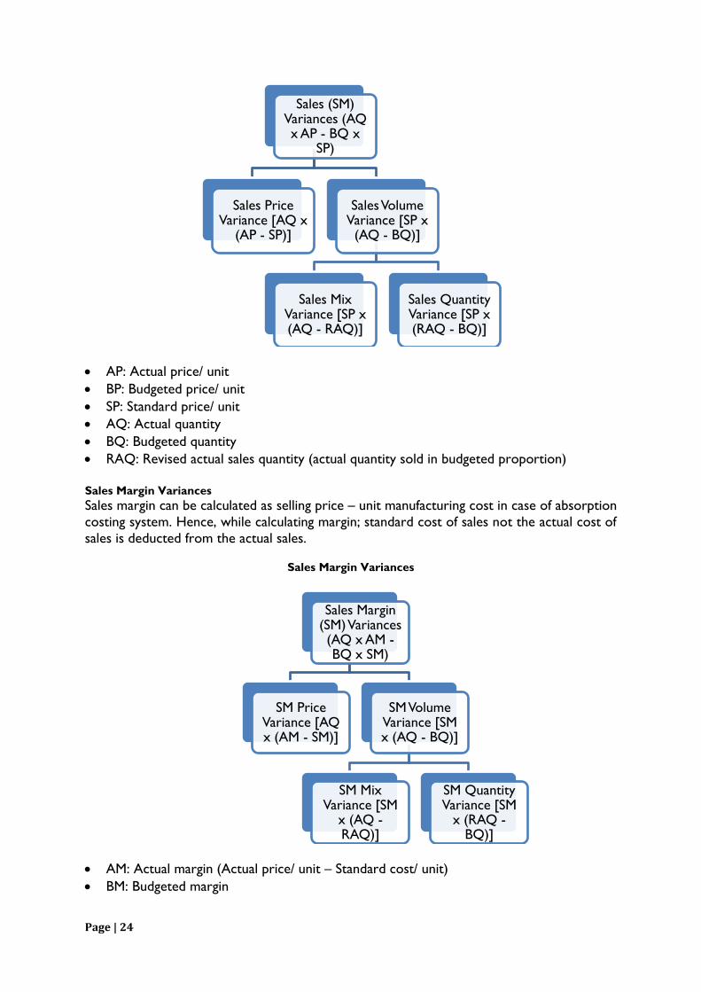
Page | 24

AP: Actual price/ unit

BP: Budgeted price/ unit

SP: Standard price/ unit

AQ: Actual quantity

BQ: Budgeted quantity

RAQ: Revised actual sales quantity (actual quantity sold in budgeted proportion)

Sales Margin Variances Sales margin can be calculated as selling price – unit manufacturing cost in case of absorption

costing system. Hence, while calculating margin; standard cost of sales not the actual cost of

sales is deducted from the actual sales.

Sales Margin Variances

AM: Actual margin (Actual price/ unit – Standard cost/ unit)

BM: Budgeted margin

Sales (SM) Variances (AQ x AP - BQ x

SP)

Sales Price Variance [AQ x

(AP - SP)]

Sales Volume Variance [SP x

(AQ - BQ)]

Sales Mix Variance [SP x (AQ - RAQ)]

Sales Quantity Variance [SP x (RAQ - BQ)]

Sales Margin (SM) Variances (AQ x AM - BQ x SM)

SM Price Variance [AQ x (AM - SM)]

SM Volume Variance [SM x (AQ - BQ)]

SM Mix Variance [SM

x (AQ - RAQ)]

SM Quantity Variance [SM

x (RAQ - BQ)]

Page | 25

SM: Standard margin (Standard price/ unit – Standard cost/ unit)

Reporting of Variances

After computation of variances, it becomes utmost necessary to report them on a prompt and periodic basis to the concerned executives, so that the causes behind the variances can

be identified and appropriate corrective measures can be taken to avoid similar adverse

variances in future with a view to fulfill the objective of cost control. Hence, these reports

should give due emphasis to standard cost performance and proximity of actual cost

performance from the standard; the magnitude of variances; and reasons for such variance.

Reporting must be made based on the principle of management by exception (MBE).

Reconciliation of profit

Variances are prepared based on standard/ budgeted and actual data. Sometimes, we are

provided with variances and actual data and we may have to compute the budgeted profit

and reconcile the budgeted profit with the actual one. The process of reconciliation is

shown below:

Reconciliation Statement (Absorption Costing Method)

Particulars Rs. Rs. Rs.

Budgeted Profit (Budgeted quantity x standard margin) XXX

Material cost variances

(a) Material price variance

(b) Material usage variance

(i) Material mix variance

(ii) Material yield variance

XXX

XXX

XXX

XXX

XXX

Labor cost variance

(a) Labor rate variance

(b) Labor idle time variance

(c) Labor efficiency variance

(i) Labor mix variance

(ii) Labor sub-mix efficiency variance

XXX

XXX

XXX

XXX

XXX

XXX

Variable overhead cost variance

(a) Variable overhead expenditure variance

(b) Variable overhead efficiency variance

XXX

XXX

XXX

Fixed overhead cost variance

(a) Fixed overhead expenditure variance

(b) Fixed overhead volume variance

(i) Fixed overhead capacity variance

(ii) Fixed overhead efficiency variance

XXX

XXX

XXX

XXX

XXX

Sales margin variance (in terms of profit)

(a) Sales margin price variance

(b) Sales margin volume variance

(i) Sales margin mix variance

(ii) Sales margin quantity variance

XXX

XXX

XXX

XXX

XXX

Actual profit XXX

Note:

Page | 26

1. If reconciliation statement is to be prepared from standard profit (actual quantity x

standard margin), standard margin volume variances will not be applicable. So, only sales

margin price variance is to be adjusted.

Problem 3: Particulars Budget Actual Variances

Sales/ production (units) 200000 165000 (35000) Sales (Rs.) 2100000 1692900 (407100) Less: Variable cost (Rs.) 1266000 1074150 191850 Less: Fixed cost (Rs.) 315000 330000 (15000) Profit 519000 288750 (230250)

Prepare a reconciliation of budgeted profit to actual profit using absorption costing

approach.

Solution: Workings:

Standard margin: Rs. 519000

Average standard margin/ unit = Rs. 519000/ 200000 units = Rs. 2.595

Actual sales price/ unit: Rs. 1692900/ 165000 units = Rs. 10.26

Standard variable cost/ unit: Rs. 1266000/ 200000 units = Rs. 6.33

Standard cost/ unit: (Rs. 1266000 + Rs. 315000)/ 200000 units = Rs. 7.905

Actual cost/ unit: (Rs. 1074150 + Rs. 330000)/ 165000 units = Rs. 8.51

Actual margin/ unit = Rs. 10.26 - Rs. 7.905 = Rs. 2.355

Actual variable cost/ unit: Rs. 1074150/ 165000 units = Rs. 6.51

Standard fixed cost/ unit: Rs. 315000/ 200000 units = Rs. 1.575

Calculation of variances

1. Sales margin variances

(a) Sales margin price variance = (AM/unit - SM/unit) x AQ = [(Rs. 2.597 – Rs. 2.357)] x

165000 units = Rs. 39600 (A)

(b) Sales margin volume variance = SM x (AQ – BQ) = Rs. 2.597 x (165000 – 200000) =

Rs. 90825

2. Variable overhead variances

(a) Variable cost variance: standard variable cost/ unit x AQ – actual variable overhead =

Rs. 6.33 x 165000 – Rs. 1074150 = Rs. 29700 (A)

3. Fixed overhead variances

(a) Fixed overhead expenditure variances: budgeted overhead – actual overhead = Rs.

315000 – Rs. 330000 = Rs. 15000 (A)

(b) Fixed overhead volume variance: absorbed overhead – budgeted overhead = Rs.

1.575 x 165000 – Rs. 315000 = Rs. 55125 (A)

Reconciliation Statement (under absorption costing)

Particulars Rs. Rs.

Budgeted Profit (Budgeted quantity x standard

margin) 519000

Variable overhead cost variance (A) (29700)

Fixed overhead expenditure variance (A) Fixed overhead volume variance (A)

(15000) (55125)

Fixed overhead cost variance (A) (70125)

Page | 27

Sales margin volume variance (A) (90825)

Sales margin price variance (A) (39600)

Sales margin variance (A) (130495)

Actual profit (reconciled) 288750

Investigation of variances

Investigation of variances is a conclusive step after calculation of variances that decisively

point out the exact cause behind a favorable or adverse variance and provide implications

for behavioral, motivational and inter-departmental changes that may be implemented to

control the variance. However, a variance does not always mean an ‘out-of-control’

situation. Hence, before undergoing investigation, the management accountant must make the management aware about the associated cost and benefit of the process.

Factors governing investigation

Variance is a difference of estimates from the actual. Investigation depends upon certain

factors within the organization:

(a) Size: If the average estimate is slightly different from the actual, the company may not

undertake investigation. In fact, the company should set a limit of the variance amount. If

the variance of a particular parameter goes beyond that limit, then only the investigation

should be undertaken.

(b) Type: adverse variance is given more priority for investigation as compared to the favorable variances.

(c) Cost: cost associated with the investigation process should be lower than the benefit

associated with it.

(d) Pattern: if the variance of a particular parameter is worsening for last few years,

investigation of the same should be undergone.

(e) Budgetary process: if the budgetary process is uncontrollable or unrealistic, then

investigation of the entire budgetary process should be undertaken instead of

investigation of a particular parameter.

Process of investigation

Rule of Thumb Method:

In order to investigate a variance, the first step is to set a limit for the variance investigation.

This limit may be an arbitrary limit based on amount of variance or may be as a percentage

of cost (say 10%) based on managerial judgments. If the standard usage for a particular

component is 10 kg/ unit and actual output is 1000 units, then the variance would not be

investigated if the actual usage is between 10% of the standard usage (9000 to 11000 kg).

Statistical Control Chart

Statistical control charts are mainly used to maintain statistical quality control of products

and services. However, they may also be used to identify out-of-control observations in

variance investigations. Each observation (say labor usage in an hour) is plotted on a chart

which is prepared based on past series of information assumed to follow normal

distribution. Hence, based on past series of information, population mean () and SD () of a parameter is determined. Based on normal distribution table, 68.27% of the observation

would fall between the ranges of +; 95.45% of the observations would fall within the

range of + 2; and 99.8% of the observations would fall within the range of + 3. For example, in an organization, there are three projects – A, B, and C. The control range

considered is + 2. Now, observations under these three projects are plotted on the

statistical control chart as follows:

Page | 28

*Source: ICAI Study Mat

It is observed that observations under Project A fall within the range of + 2, while in

case of Project B, two observations are out of control. Hence, investigation of variances is

required for those two observations. While all observations are within the control range

under Project C, the observations seem to slowly cross the range. Hence, the project may

be considered for investigation based on the trend of observations.

Cost-benefit Analysis

Cost benefit analysis involves comparing the expected cost to the company if they undergo

investigation of variance and expected cost to the company if they don’t.

Now, two mutually exclusive states are possible in variance investigation – ‘in-control’

(where variance occurred due to random fluctuations from the expected result) and ‘out-of-

control’ (where corrective actions are required to be taken). If the underlying variance

follows normal distribution, probability of the variance being an ‘in-control’ (P1) can be

determined based on normal distribution theory. The probability of variance being ‘out-of-

control’ (P2) is equal to (1-P1).

Example: Average time required for producing an output is 2.5 hours is normally distributed

with a standard deviation (SD) of 15 minutes (derived from average of a series from past

experience under close supervision). Actual time taken for production of 1000 units is 3000

hours. Hence, time taken to produce 1 unit is 3 hours. Since, the distribution is normal, the test

statistics (Z) is calculated as follows: Z = x - / = (3-2.5)/0.25 = 2. P (Z=2) = 0.9772. Hence,

probability of completing the project in more than 3 hours is (1-0.9772) = 0.0228 or 2.28%.

Hence, the probability of time taken for completing a unit in more than 3 hours (being out-of-

control) is 2.28%. If the probability goes beyond 2.28%, the variance is to be investigated.

There are four types of cost associated with an investigation process:

(a) Cost of investigation (C)

(b) Cost of correction (M)

(c) Cost of process per period being out-of-control (P)

(d) Cost of process allowed to remain out-of-control (L)

Expected cost of undergoing investigation and not undergoing investigation can be evaluated

as follows: Action In-control probability (P1) Out-of-control probability (P2)

Investigate C C + M + P

Do not investigate - L

Page | 29

Expected cost of undergoing investigation: P1 x C + P2 x (C+M+P)

Expected cost of not undergoing investigation: P2 x L

Decision about investigation is taken as follows:

If expected cost of undergoing investigation > expected cost of not undergoing investigation => Do not undergo investigation

If expected cost of undergoing investigation < expected cost of not undergoing

investigation => Undergo investigation

If expected cost of undergoing investigation = expected cost of not undergoing

investigation => Take decision about investigation about managerial judgment

The break-even probability is the level where,

Expected cost of undergoing investigation = Expected cost of not undergoing investigation

Or, P1 x C + P2 x (C+M+P) = P2 x L

Or, (1-P2) x C + P2 x (C+M+P) = P2 x L

Or, C + P2 x (M+P) = P2 x L

Or, P2 = C/ [L – (M+P)]

P2 is the probability of variance being out-of-control

C is the cost of investigation

L – (M+P) is the benefit obtained from investigation

Hence, investigation is to be carried out if probability of being out of control > cost of

investigation/ benefit of investigation

Problem 4:

A company using a detailed system of standard costing finds that the cost of investigation of

variances is Rs. 20,000. If after investigation, an out of control situation is discovered, the

cost of correction is Rs. 30,000. Cost of process per period out of control is Rs. 24000. If

no investigation made, the present value of extra cost involved is Rs. 150000. The

probability of the process being in control is 0.82 and the probability of the process being

out of control is 0.18. You are required to advise whether investigation of the variances

should be undertaken or not. Calculate the probability at which it is desirable to institute

investigation into variances.

Solution: Pay-off matrix

Action In-control (0.82) Out-of-control (0.18)

Investigate Rs. 20000 Rs. 20000 + Rs. 30000 + Rs. 24000 = Rs. 74000

Do not investigate - Rs. 150000

If investigation is done, the expected cost is: Rs. 20000 x 0.82 + Rs. 74000 x 0.18 = Rs. 29720

If investigation is not done, the expected cost is: Rs. 150000 x 0.18 = Rs. 27000

Hence, it is advisable not to investigate.

The probability at which it is desirable to institute investigation is the point where the

expected costs of each action are same.

Cost of investigation (C): Rs. 20000

Page | 30

Cost of correction (M): Rs. 30000

Cost of process per period out of control (P): Rs. 24000

Extra cost if no investigation (L): Rs. 150000

Probability of being in control = P1 = (1 – P2)

Probability of being out-of-control = P2

Expected cost of investigation: P1 x C + P2 x (C+M+P) = (1-P2) x Rs. 20000 + P2 x 74000 =

54000 P2 + 20000.

Expected cost if investigation is not made: P2 x L = Rs. 150000 P2

Expected cost from the actions equal

Hence, 54000 P2 + 20000 = 150000 P2

P2 = [20000/ (150000 – 54000)] = 0.21

Hence, investigation is desirable when probability of being out-of-control is more than 0.21.

In the current situation, that probability is 0.18. Hence, the decision not to investigate is apt.

Suggested Readings: 5. B. Banerjee, Cost Accounting, PHI, New Delhi

6. Ashish Bhattacharya, Cost Accounting, PHI, New Delhi

7. Charles T. Horngreen, et al. Introduction to Management Accounting, Prentice Hall of India

8. Colin Drury, Management and Cost Accounting, Thomson Learning

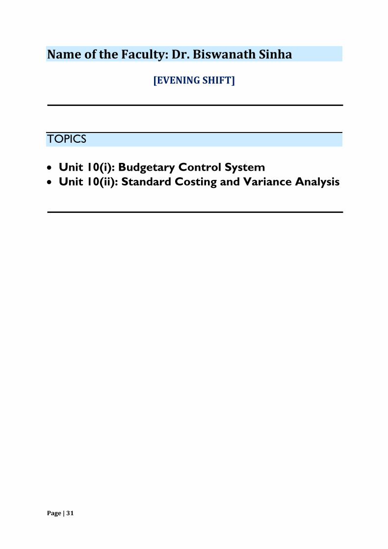
Page | 31

Name of the Faculty: Dr. Biswanath Sinha

[EVENING SHIFT]

TOPICS

Unit 10(i): Budgetary Control System

Unit 10(ii): Standard Costing and Variance Analysis

1 (Compiled by Dr.Biswanath Sinha)

Strategic Cost and Management Accounting

Module (ii) (Evening section)

Standard costing and Variance analysis:

1. Already taught in class:

a) Introduction: Concept, steps involved, types of standard, material and labour cost variances.

b) Fixed and variables overhead variance: Problem solved

c) Sales Variance: (i) The value method ( Problem solved)

(ii) The profit method (Problem solved)

2. Investigation of variances:

Not all variances are investigated by management. Investigation decisions have a cost. Hence, they

have to decide which areas have to be investigated. An investigation should only be undertaken if

the benefits expected from the investigation exceeds the cost of searching for and correcting the

source of variance. This method is also known as cost-benefit analysis.

Example:

Cost of investigation of variance (I) = INR 12,800

Cost of correction of out of control process (C) = INR 32,000

Cost of allowing the process to remain out of control (O) = INR 1, 60,000

Probability of being in control = 0.95

Probability of being out of control = 0.05

(Q1) Should investigation of variance be undertaken or not?

(Q2) Find out the break-even probability

Solution (Q1):

The expected value of each action will be:

a) Investigate E(a1) = PI + (1-P)*(I+C)

b) Do not investigate E(a2) = (1-P)*O

Therefore, Expected value of investigation E (a1) = (0.95*12,800) + (1-0.95)*(12,800+32,000)

= INR 14,400

Expected value of not investigation E (a2) = 0.05*1, 60,000

= INR 8,000

2 (Compiled by Dr.Biswanath Sinha)

Since the cost to investigate (14,400) is more than the cost of not investigating (8000); hence the

advice to management will be not to investigate.

Solution to Q2:

Let P1 be the break-even probability (i.e., cost of investigation = cost of not investigation)

E (a1) = E (a2)

Or, (P1*12800) + (1-P1)*(12800+32000) = (1-P1)*(1, 60,000)

After solving the equation we get;

P1 = 0.9 or 90%

Therefore, the break-even probability is 90%.

3 (Compiled by Dr.Biswanath Sinha)

Budgetary Control System:

A) Introduction:

Budgetary control is a system of planning and controlling cost. For this purpose the following steps

are involved:

Establishment of budget

Measurement of actual performance

Comparison of actual performance with budgeted performance to ascertain variances

Analysis of the causes of variation and reporting to the right people to take right action at

the right moment

The objectives of budgetary control are normally to plan and control the income and expenditure of

manufacturing and trading operations; capital expenditure; expenditure on research and

development and financing of a business to ensure adequate working capital. In small companies the

preparation of budget is the responsibility of the cost and management accountant. But in large

companies preparation of budget is done by a budget committee which consists of sales manager,

production manager, purchase manager, accountant etc. following the guidelines given in the

budget manual. The budget manual should provide the detailed procedure for preparation,

development and control of each functional budget like sales budget, production budget etc.

In the preparation of budget, principle budget factor (i.e., a factor is of such importance that it

influences all other budgets) is the starting point and all other budgets must be centered around. For

example: A factory can produce (Maximum capacity) 40,000 units per year of a particular product.

But the demand for the product in the market is only 30,000 units per year. Hence, demand for sales

is the limiting factor. Therefore, sales budget must be prepared first and other budgets such as

production budget, material purchase budget etc. should follow the sales budget.

The traditional budgeting gives more emphasis on the financial aspect than the physical aspect or

performance. In this context the concept of Performance Budgeting has been introduced.

Performance Budgeting is a technique of presenting the budget for cost and revenue in terms of

function, programs and activities and correlating the physical and financial aspect of the individual

items comprising the budget. Thus, performance budgeting aims at establishing a relationship

between the inputs and the outputs. Hence, under this technique the emphasis is more on the

functions of the organization, the program to discharge these functions and the activities which will

be involved in undertaking these programs ,i.e., the main focus is; the purpose for which the

expenditure is being incurred and not the items of expenditure.

Moreover, for better resource allocation and control, another new technique Zero Based Budgeting

has also been introduced. This technique starts with the premise that the budget for the next period

is zero so long the demand for a function, process, project or activity is not justified for each rupee.

Thus, each functional manager is required to carry out cost benefit analysis of each of the activities

for which he is responsible. For this purpose the following steps are normally undertaken:

To develop decision package

To evaluate all decision packages and rank them in order of importance through cost benefit

analysis and allocated resource accordingly

4 (Compiled by Dr.Biswanath Sinha)

B) Functional Budgets:

Functional budgets include:

Sales budget

Production budget

Purchase budget

Wages budget

Manpower budget

Example to prepare a functional budget is given below:

5 (Compiled by Dr.Biswanath Sinha)

Solution: